Joseph Tabrikian Signal Processing Laboratory
Department of Electrical and Computer Engineering
Ben-Gurion University of the Negev
Involved collaborators and Research Assistants: Prof. R. Shavit, Prof. H. Messer, Dr. I. Bilik, I. Bekkerman, W. Huleihel, M. Teitel, N. Sharaga, O. Isaacs
BGU Radar Symposium 2016
Cognitive MIMO Radar
Outline
MIMO radar at a glance
Cognitive radar - introduction
Cognitive MIMO radar for beamforming and detection
Conclusion
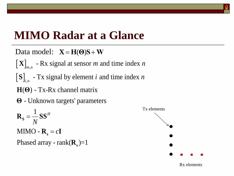
MIMO Radar at a Glance
Data model: ( ) X H Θ S W
,
,
- Rx signal at sensor and time index
- Tx signal by element and time index
( ) - Tx-Rx channel matrix
- Unknown targets' parameters
1
MIMO -
Phased array - rank( )=1
m n
i n
H
m n
i n
N
c
S
s
s
X
S
H Θ
Θ
R SS
R I
R
Tx elements
Rx elements
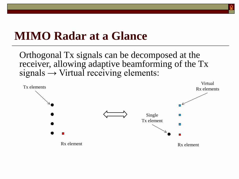
MIMO Radar at a Glance
Orthogonal Tx signals can be decomposed at the receiver, allowing adaptive beamforming of the Tx signals → Virtual receiving elements:
Tx elements
Rx element
Single
Tx element
Rx element
Virtual
Rx elements
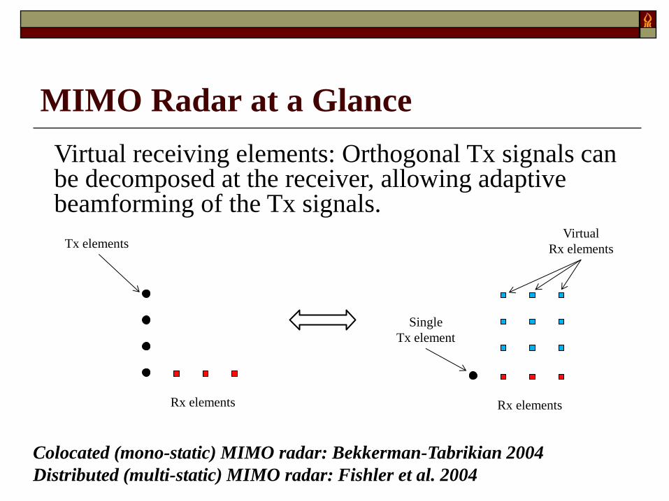
MIMO Radar at a Glance
Virtual receiving elements: Orthogonal Tx signals can be decomposed at the receiver, allowing adaptive beamforming of the Tx signals.
Tx elements
Rx elements
Colocated (mono-static) MIMO radar: Bekkerman-Tabrikian 2004
Distributed (multi-static) MIMO radar: Fishler et al. 2004
Single
Tx element
Rx elements
Virtual
Rx elements
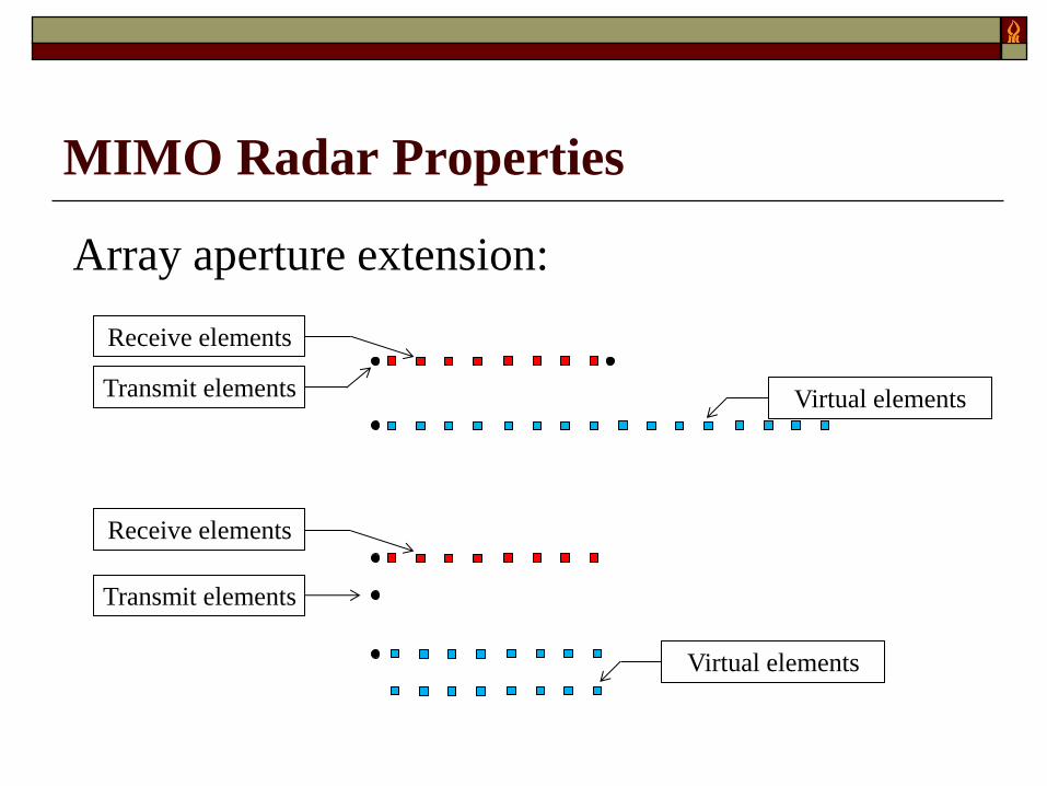
MIMO Radar Properties
Array aperture extension:
Virtual elements
Transmit elements
Receive elements
Receive elements
Transmit elements
Virtual elements
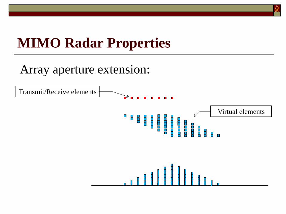
MIMO Radar Properties
Array aperture extension:
Virtual elements
Transmit/Receive elements
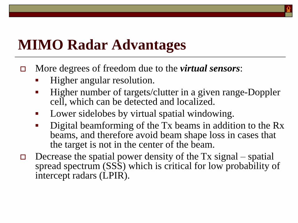
MIMO Radar Advantages
More degrees of freedom due to the virtual sensors:
Higher angular resolution.
Higher number of targets/clutter in a given range-Doppler cell, which can be detected and localized.
Lower sidelobes by virtual spatial windowing.
Digital beamforming of the Tx beams in addition to the Rx beams, and therefore avoid beam shape loss in cases that the target is not in the center of the beam.
Decrease the spatial power density of the Tx signal – spatial spread spectrum (SSS) which is critical for low probability of intercept radars (LPIR).
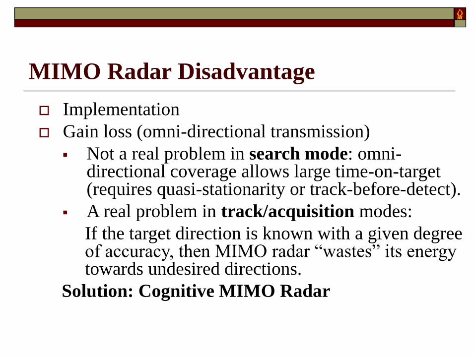
MIMO Radar Disadvantage
Implementation
Gain loss (omni-directional transmission)
Not a real problem in search mode: omni-directional coverage allows large time-on-target (requires quasi-stationarity or track-before-detect).
A real problem in track/acquisition modes:
If the target direction is known with a given degree of accuracy, then MIMO radar “wastes” its energy towards undesired directions.
Solution: Cognitive MIMO Radar
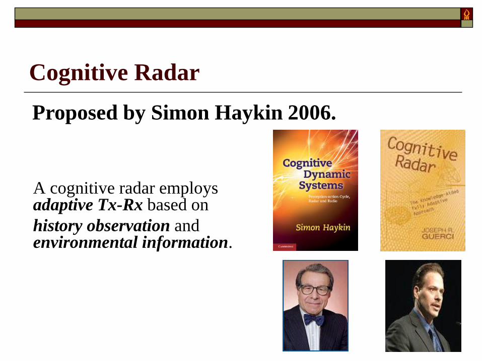
Cognitive Radar
Proposed by Simon Haykin 2006.
A cognitive radar employs adaptive Tx-Rx based on
history observation and environmental information.
Cognitive Radar
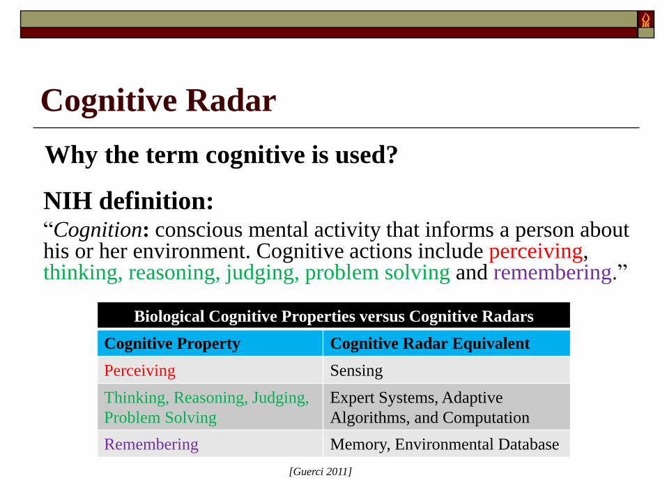
Why the term cognitive is used?
Biological Cognitive Properties versus Cognitive Radars
Cognitive Property Cognitive Radar Equivalent
Perceiving Sensing
Thinking, Reasoning, Judging,
Problem Solving
Expert Systems, Adaptive
Algorithms, and Computation
Remembering Memory, Environmental Database
[Guerci 2011]
NIH definition: “Cognition: conscious mental activity that informs a person about his or her environment. Cognitive actions include perceiving, thinking, reasoning, judging, problem solving and remembering.”
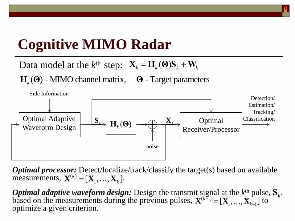
Cognitive MIMO Radar
Optimal Adaptive
Waveform Design Optimal
Receiver/Processor
Detection/
Estimation/
Tracking/
Classification
noise
( )kH Θ
Side Information
kS kX
Data model at the kth step: ( )k k k k X H Θ S W
( ) - MIMO channel matrix, - Target parameterskH Θ Θ
Optimal processor: Detect/localize/track/classify the target(s) based on available measurements, .
Optimal adaptive waveform design: Design the transmit signal at the kth pulse, , based on the measurements during the previous pulses, to optimize a given criterion.
( )
1[ , , ]k
kX X X
kS( 1)
1 1[ , , ]k
k
X X X
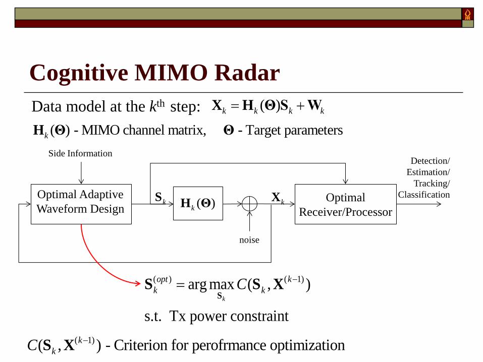
Cognitive MIMO Radar
Optimal Adaptive
Waveform Design Optimal
Receiver/Processor
Detection/
Estimation/
Tracking/
Classification
noise
( )kH Θ
Side Information
kSkX
Data model at the kth step: ( )k k k k X H Θ S W
( ) - MIMO channel matrix, - Target parameterskH Θ Θ
( ) ( 1)arg max ( , )
s.t. Tx power constraint
k
opt k
k kC S
S S X
( 1)( , ) - Criterion for perofrmance optimizationk
kC S X
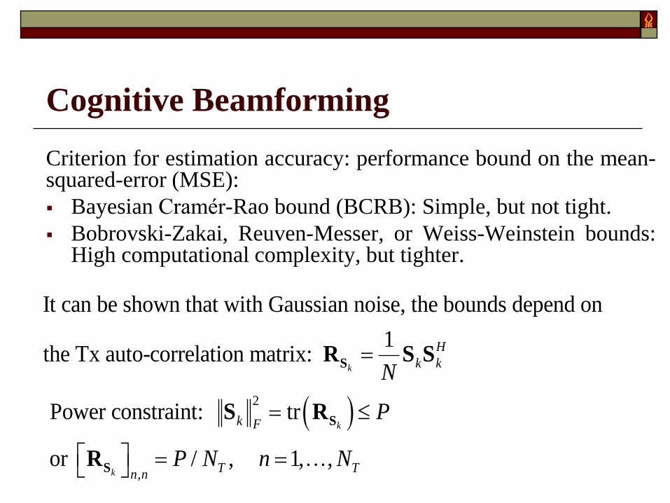
Cognitive Beamforming
Criterion for estimation accuracy: performance bound on the mean-squared-error (MSE):
Bayesian Cramér-Rao bound (BCRB): Simple, but not tight.
Bobrovski-Zakai, Reuven-Messer, or Weiss-Weinstein bounds: High computational complexity, but tighter.
2
,
Power constraint: tr
or / , 1, ,
k
k
k F
T Tn n
P
P N n N
S
S
S R
R
It can be shown that with Gaussian noise, the bounds depend on
1the Tx auto-correlation matrix:
k
H
k kN
SR S S
Cognitive Beamforming
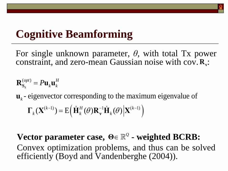
For single unknown parameter, θ, with total Tx power constraint, and zero-mean Gaussian noise with cov. :
( )
( 1) 1 ( 1)
- eigenvector corresponding to the maximum eigenvalue of
( ) E ( ) ( )
k
opt H
k k
k
k H k
k k k
P
S
v
R u u
u
Γ X H R H X
vR
Vector parameter case, - weighted BCRB:
Convex optimization problems, and thus can be solved efficiently (Boyd and Vandenberghe (2004)).
QΘ
Example – Cognitive Beamforming
2
2 2
:
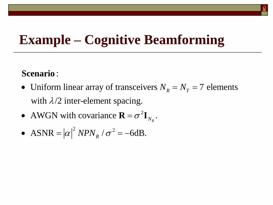
Uniform linear array of transceivers 7 elements
with /2 inter-element spacing.
AWGN with covariance .
ASNR / 6dB.
R
R T
N
R
N N
NPN
Scenario
R I
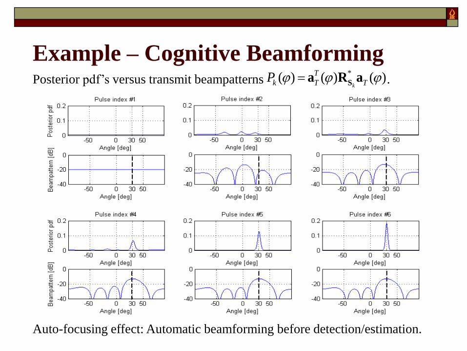
Posterior pdf’s versus transmit beampatterns .
Auto-focusing effect: Automatic beamforming before detection/estimation.
Example – Cognitive Beamforming *( ) ( ) ( )
k
T
k T TP Sa R a
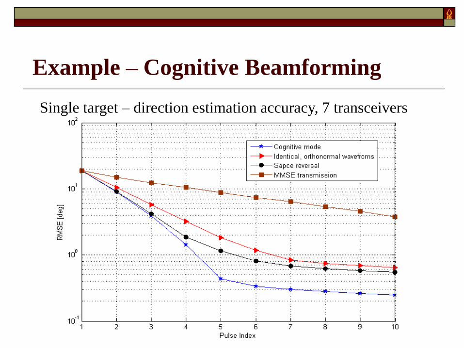
Single target – direction estimation accuracy, 7 transceivers
Example – Cognitive Beamforming
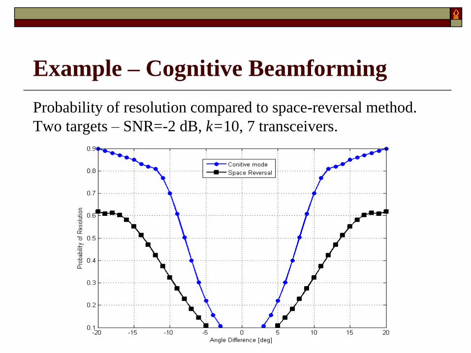
Probability of resolution compared to space-reversal method.
Two targets – SNR=-2 dB, k=10, 7 transceivers.
Example – Cognitive Beamforming
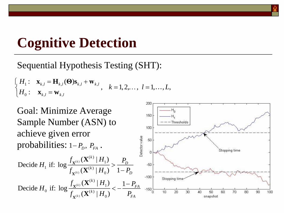
Cognitive Detection
Sequential Hypothesis Testing (SHT):
Goal: Minimize Average
Sample Number (ASN) to
achieve given error
probabilities: .
, , ,
, ,
1 ,
0
: ( ), 1, ,
: 1,2
,
,
,
k l k l k l
k l
k l
k l
Hl L
Hk
x H Θ w
x w
s
1 , D FAP P
( )
( )
( )
( )
( )
1
( )
0
( )
1
(
1
0 )
0
Decide if:
De
( | )log
(
cide
| ) 1
(
| ) 1log
( | )if:
k
k
k
k
k
D
k
D
k
FA
k
FA
f H PH
H
f H P
f H P
f H P
X
X
X
X
X
X
X
X
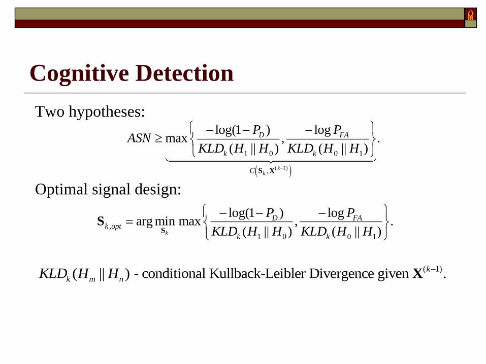
Cognitive Detection
Two hypotheses:
Optimal signal design:
( 1),
1 0 0 1
log(1 ) logmax , .
( || ) ( || )
kk
D FA
k k
C
P P
KLD H H KLASN
D H H
S X
1 0
,
0 1
log(1 ) logarg min max , .
( || ) ( || )k
D FAk opt
k k
P P
KLD H H KLD H H
S
S
( 1)( || ) - conditional Kullback-Leibler Divergence given .k
k m nKLD H H X
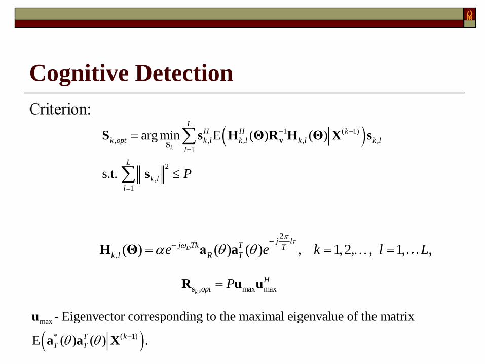
Cognitive Detection
( 1)
, ,
1
,
1
,
2
1
, ,arg min E
s.t
( )
(
.
)
k
H H
k l k l k l
Lk
k opt k l
l
L
k l
l
P
vS
H Rs Θ Θ
s
sHS X
2
, ) ) 1,2, , ,( ) ( ( , 1,Dj l
Tk Tk l
j T
R T e k l Le
H aΘ a
, max maxk
H
opt Ps
R u u
max
* ( 1)
Eigenvector corresponding to the maximal eigenvalue of the matrix
( (
-
E ) ) .T k
T T
u
a a X
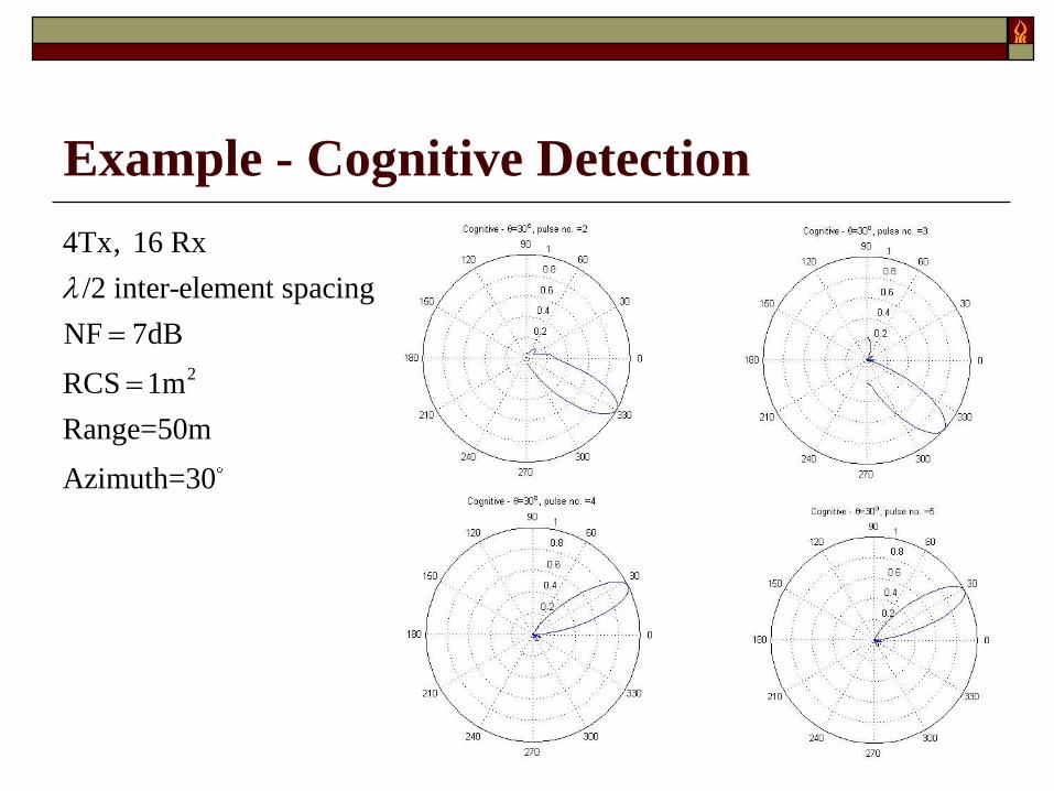
Example - Cognitive Detection
2
4Tx, 16 Rx
/2 inter-element spacing
NF 7dB
RCS 1m
Range=50m
Azimuth=30
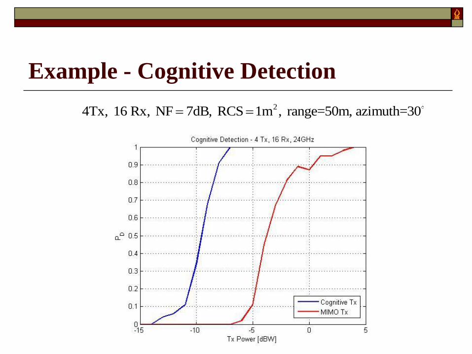
Example - Cognitive Detection
24Tx, 16 Rx, NF 7dB, RCS 1m , range=50m, azimuth=30
Conclusions and Future Research
MIMO radar offers great advantages but needs to be used with care.
In cognitive MIMO radar, Tx signal auto-correlation matrix is adaptively optimized. The optimized signal is not necessarily orthogonal (MIMO) or fully correlated (phased array).
Two new cognitive Tx beamforming approaches were presented to optimize: localization accuracy and detection performance
This approach provides an automatic focusing array: beamforming before detectionqestimation.
Future research:
Considering other criteria, such as probability of resolution, or target classification performance.

Thank you!
Recommended

![Hard Decision-Based PWM for MIMO-OFDM Radar · 2. MIMO-OFDM Radar Signal Model-Based PWM 2.1. MIMO-OFDM Radar Systems Structure In [1], OFDM technique has the advantage of combating](https://img.pdfslide.us/doc/110x75/5e6a685a5002aa073940e3bf/hard-decision-based-pwm-for-mimo-ofdm-radar-2-mimo-ofdm-radar-signal-model-based.jpg)