Climate warming and decreasing total column ozone
over the Tibetan Plateau during winter and spring
By JIANKAI ZHANG1, WENSHOU TIAN1*, FEI XIE2, HONGYING TIAN1, JIALI LUO1,
JIE ZHANG1, WEI LIU1 and SANDIP DHOMSE3, 1Key Laboratory for Semi-Arid Climate
Change of the Ministry of Education, College of Atmospheric Sciences, Lanzhou University, Lanzhou, China;2State Key Laboratory of Numerical Modeling for Atmospheric Sciences and Geophysical Fluid Dynamics,
Institute of Atmospheric Physics, Chinese Academy of Sciences, Beijing, China; 3School of Earth and
Environment, University of Leeds, Leeds, UK
(Manuscript received 22 November 2013; in final form 1 April 2014)
ABSTRACT
The long-term trends of the total column ozone (TCO) over the Tibetan Plateau (TP) and factors responsible
for the trends are analysed in this study using various observations and a chemistry�climate model (CCM).
The results indicate that the total column ozone low (TOL) over the TP during winter and spring is deepening
over the recent decade, which is opposite to the recovery signal in annual mean TCO over the TP after
mid-1990s. The TOL intensity is increasing at a rate of 1.4 DU/decade and the TOL area is extending with
50,000 km2/decade during winter for the period 1979�2009. The enhanced transport of ozone-poor air into the
stratosphere and elevated tropopause due to the rapid and significant warming over the TP during winter
reduce ozone concentrations in the upper troposphere and lower stratosphere and hence lead to the deepening
of the TOL. Based on the analysis of the multiple regression model, the thermal dynamical processes associated
with the TP warming accounts for more than 50% of TCO decline during winter for the period 1979�2009.The solar variations during 1995�2009 further enlarge ozone decreases over the TP in the past decade.
According to the CCM simulations, the increases in NOx emissions in East Asia and global tropospheric
N2O mixing ratio for the period 1979�2009 contribute to no more than 20% reductions in TCO during this
period.
Keywords: total column ozone, Tibetan Plateau, climate warming, nitrous oxide
1. Introduction
Due to its strong ultraviolet absorption and greenhouse
effect, ozone plays an important role in the atmospheric
radiation balance (Forster and Shine, 1997). As a result
of human activities, global total column ozone (TCO) has
decreased remarkably over past decades. However, since the
signing of the Montreal Protocol in 1987, some chlorofluor-
ocarbons (CFCs) and other ozone-depleting substances
(ODSs) in the atmosphere are decreasing steadily, and
the stratospheric ozone is expected to recover in the future
(WMO, 2011). Recent chemistry�climate model simulations
indicate that the recovery of ozone over the lower latitudes is
different from that over higher latitudes (Austin et al., 2010).
The Tibetan Plateau (TP), the highest topography in the
world, not only has a significant impact on the atmospheric
circulation and climate system in East Asia (e.g. Yanai et al.,
1992; Ye andWu, 1998) but also has a remarkable influence
on the ozone distribution (e.g. Tian et al., 2008). Under the
situation of global ozone recovery and climate changes,
whether the ozone over the TP exhibits trends similar to
those over other regions of the earth is a question worth
investigating. Zhou et al. (1995) found from the Total Ozone
Mapping Spectrometer (TOMS) satellite measurements that
there is a remarkable low TCO centre over the TP in the
summer, which is called as the ‘ozone valley’. This phenom-
enon was also found in ozonesonde observations at Lhasa
station of the TP (Tobo et al., 2008). A question arises as to
whether the so-called ‘ozone valley’ over the TP is recover-
ing or deepening.
Although the mechanisms for the formation of low
TCO centre over the TP have been researched in previous
*Corresponding author.
email: [email protected]
Responsible Editor: Annica Ekman, Stockholm University, Sweden.
Tellus B 2014. # 2014 J. Zhang et al. This is an Open Access article distributed under the terms of the Creative Commons CC-BY 4.0 License (http://
creativecommons.org/licenses/by/4.0/), allowing third parties to copy and redistribute the material in any medium or format and to remix, transform, and build
upon the material for any purpose, even commercially, provided the original work is properly cited and states its license.
1
Citation: Tellus B 2014, 66, 23415, http://dx.doi.org/10.3402/tellusb.v66.23415
P U B L I S H E D B Y T H E I N T E R N A T I O N A L M E T E O R O L O G I C A L I N S T I T U T E I N S T O C K H O L M
SERIES BCHEMICALAND PHYSICALMETEOROLOGY
(page number not for citation purpose)
studies (e.g. Zou, 1996; Ye and Xu, 2003; Zheng et al., 2004;
Tian et al., 2008), less attention was paid to the ozone trend
over the TP due to the lack of long-term observations. Ye and
Xu (2003) analysed the TOMS data from 1979 to 2000 and
reported that the interannual variability of annual mean
TCO over the TP is in phase with but weaker than the
plateau’s corresponding zonal mean TCO. They also argued
that the interannual variability of TCO over the TP is
controlled by a mechanism with a scale much larger than
the topography of the TP. It is known that global ozone
abundance and its trend are mainly controlled by the ODSs
in the atmosphere and atmospheric conditions. The relative
importance of physical and chemical processes influenc-
ing the variability and long-term trend of TCO over the
TP remains unclear. Based on TOMS TCO observations,
Zou (1996) estimated a decline in TCO over the TP of
�0.7990.82 DU per year during the period 1978�1991.Ye and Xu (2003) also pointed out that the TCO at latitudes
of the TP shows an evident decline from 1979 to 2000.
However, Liu et al. (2001) used a 2-D chemistry model
to simulate the ozone trend over the TP and found that
the ozone above the TP was projected to recover after
1995.With the availability of TCO observations for a longer
period, it is worth re-examining the long-term trend of
TCO over the TP. In this paper, we use TOMS/SBUV
merged TCO data and the assimilated TCO data generated
by National Institute of Water and Atmospheric Research
(NIWA) as well as the Whole Atmosphere Community
Climate Model, version 3 (WACCM3) to analyse decadal
variations of ozone and its long-term trends over the TP,
and then compare them with those over the other regions
at the same latitude of the TP (hereafter, ‘non-TP’, unless
otherwise stated).
2. Data description and methods
The primary ozone data used in this study is monthly
mean TOMS/SBUV merged TCO data from 1979 to 2009
(http://acdb-ext.gsfc.nasa.gov/Data_services/merged/) which
is available at a horizontal resolution of 58 latitude �108longitude. The NIWA assimilated ozone column data,
which has a horizontal resolution of 18 latitude�1.258longitude and covers the time period from January in 1979
to November in 2009, is also employed. More details about
the NIWA data can be found in Bodeker et al. (2005). To
investigate vertical variations of the ozone over the TP,
330(a) (b)
310
290
270
250
350(c)
DU
DU
DU
/dec
ade
DU
/dec
ade
340
330
2
0
–2
–4
–6
–8
–10
–12
0
–2
–4
–6
–8
–10
(d)
Dec Jan
Feb
Mar Apr
May Ju
n JulAug Sep Oct
Nov
Dec Jan
Feb
Mar Apr
May Ju
n JulAug Sep Oct
Nov
310
290
270
250
320300280260240220
DU
DU
330310290270250230
1980
1984
1988
1992
1996
2000
2004
1980
1984
1988
1992
1996
2000
2004
2008
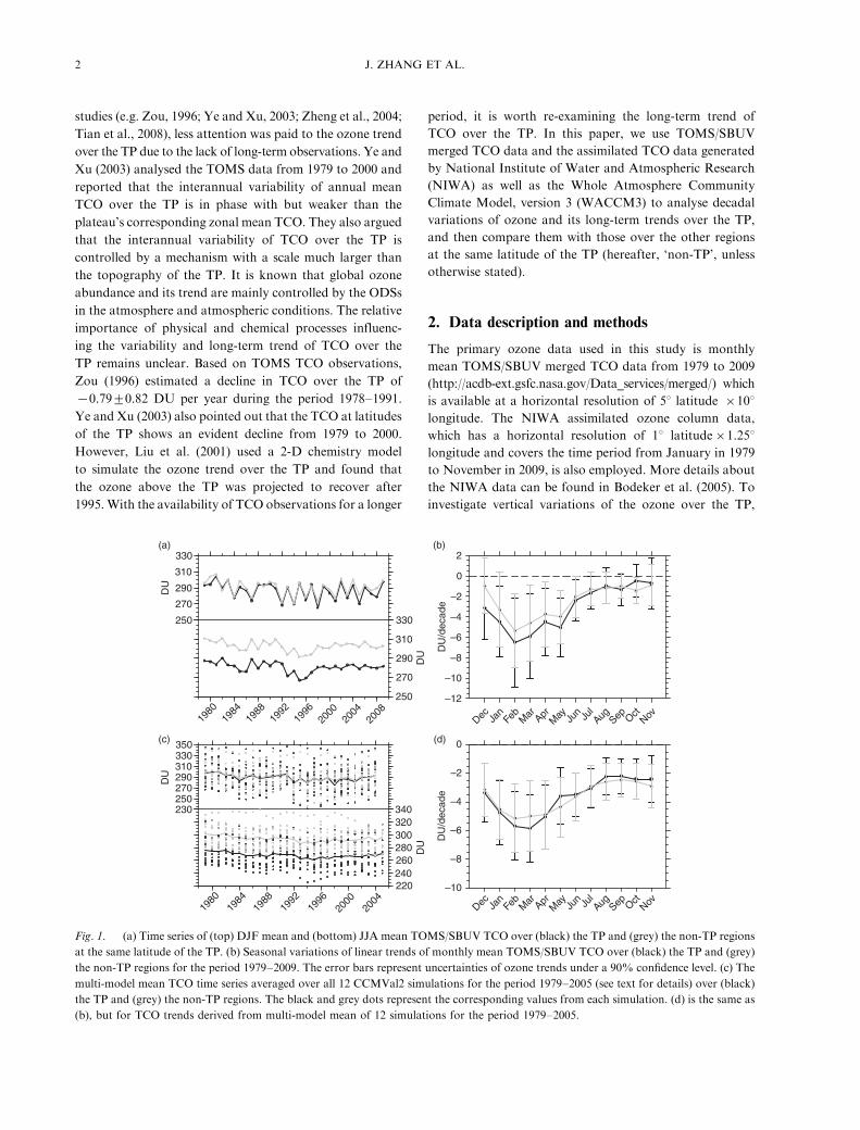
Fig. 1. (a) Time series of (top) DJF mean and (bottom) JJA mean TOMS/SBUV TCO over (black) the TP and (grey) the non-TP regions
at the same latitude of the TP. (b) Seasonal variations of linear trends of monthly mean TOMS/SBUV TCO over (black) the TP and (grey)
the non-TP regions for the period 1979�2009. The error bars represent uncertainties of ozone trends under a 90% confidence level. (c) The
multi-model mean TCO time series averaged over all 12 CCMVal2 simulations for the period 1979�2005 (see text for details) over (black)
the TP and (grey) the non-TP regions. The black and grey dots represent the corresponding values from each simulation. (d) is the same as
(b), but for TCO trends derived from multi-model mean of 12 simulations for the period 1979�2005.
2 J. ZHANG ET AL.
monthly mean ozone profiles derived from ERA-Interim
reanalysis data (http://www.ecmwf.int) and the Strato-
spheric Aerosol and Gas Experiment II (SAGE II) dataset
(ftp://ftp-rab.larc.nasa.gov/pub/sage2/v6.20) are used. The
ERA-Interim ozone data spans the time period 1979�2009and covers an altitude range from 300 to 10 hPa. Previous
studies have illustrated that ERA-Interim ozone data com-
pares well with satellite ozone observations and can be used
to analyse changes in fluxes of ozone across the tropopause
from 1979 to 2009 (Dragani, 2011; Skerlak et al., 2013).
The SAGE II ozone data is only available for 1985�2004and covers an altitude range of 15�40 km. The monthly
surface temperature observations over the TP from the
China Meteorological Administration (CMA) and the sur-
face temperatures over the Northern Hemisphere for the
period 1979�2009 from the Climatic Research Unit (CRU)
TS 3.10 datasets (http://badc.nerc.ac.uk/view/ badc.nerc.ac.
uk__ATOM__ dataent_1256223773328276) are also used.
The 3-D wind fields and the tropopause pressure are deri-
ved from the monthly ERA-Interim data for the period
1979�2009 which has a resolution of 1.58 latitude�1.58longitude.
For the purpose of understanding the impact of chemical
processes on ozone variations over the TP, theWhole Atmo-
sphere Community Climate Model, version 3 (WACCM3)
with 66 vertical levels from the surface to approximately
145 km is also employed. The WACCM3 has been ex-
tensively evaluated against various satellite data sets and
has a good representation of stratospheric chemistry and
dynamics (SPARC CCMVal 2010). The details of the model
can be found in Garcia et al. (2007). Three time-slice sim-
ulations presented in this paper were performed at a
resolution of 1.98 latitude�2.58 longitude, with interactive
chemistry enabled. The sea surface temperatures, green-
house gas values, mixing ratio lower boundary conditions
of CFCs and N2O used in the control experiment (R1) are
monthly mean climatology for the time period 1981�2005.The surface emissions of NOx (NOx�NO�NO2) in
WACCM3 are representative of those in the early 1990s
(Horowitz et al., 2003). In the experiment R2 and R3,
60N1980–1989
1980–1989
1990–1999DJF
MAM
JJA
1990–1999
2000–2009
2000–2009
1980–1989 1990–1999 2000–2009
40N
20N
60E 90E 120E 60E 90E 120E 60E 90E 120E
60E 90E 120E60E 90E 120E60E 90E 120E
60E 90E 120E
–30 –25 –20 –15 –10 –5 0 5 10 15 20 25 30
60E
TCO(DU)
90E 120E 60E 90E 120E
0
60N
40N
20N
0
60N
40N
20N
0
60N
40N
20N
0
60N
40N
20N
0
60N
40N
20N
0
60N
40N
20N
0
60N
40N
20N
0
60N
40N
20N
0
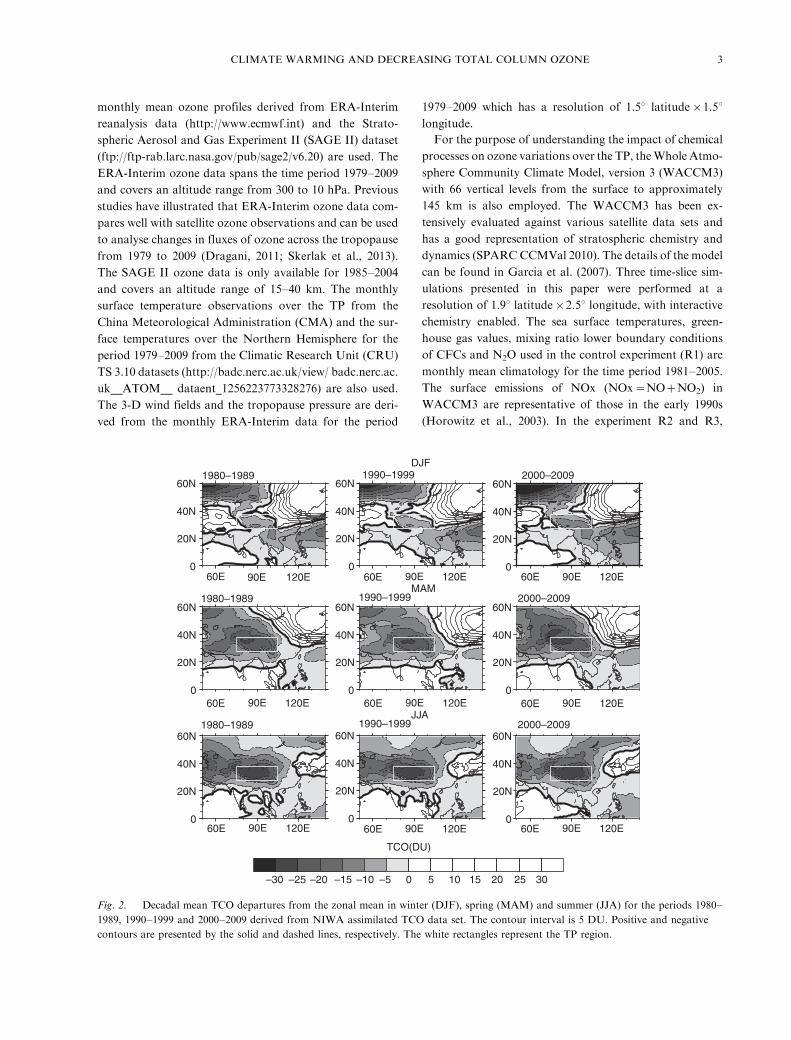
Fig. 2. Decadal mean TCO departures from the zonal mean in winter (DJF), spring (MAM) and summer (JJA) for the periods 1980�1989, 1990�1999 and 2000�2009 derived from NIWA assimilated TCO data set. The contour interval is 5 DU. Positive and negative
contours are presented by the solid and dashed lines, respectively. The white rectangles represent the TP region.
CLIMATE WARMING AND DECREASING TOTAL COLUMN OZONE 3
all configurations are the same as R1, except that the
NOx emissions in East Asia (0�908N, 90�1408E) and the
lower boundary conditions of global N2O mixing ratio are
increased by 50% and 20%, respectively. All of these three
experiments were run for 25 yr with the first 5 yr excluded for
the model ‘spin-up’ and the remaining 20 yr of data are used
for the analysis.
3. Long-term trends of TCO over the TP
Figure 1a shows long-term variations of December�January�February (DJF) mean and June�July�August
(JJA) mean TOMS/SBUV TCO data averaged over the TP
(27.5�37.58N, 75�1058E). The corresponding TCO values
averaged over the non-TP are also shown for comparison.
Consistent with the results in the earlier studies (e.g. Ye
and Xu, 2003; Tian et al., 2008), the DJF mean TCO over
the TP is close to that over the non-TP, while in boreal
summer, the TCO over the TP is up to 20 DU lower than
that over the non-TP. In phase with the global ozone trend
(e.g. Angell and Free, 2009; Krzyscin et al., 2012), the
annual mean TCO over the latitude of the TP shows an
evident decline from 1979 to the mid-1990s and begins to
recover thereafter (not shown). The recovery signal in the
annual mean TCO over the TP for the period 1995�2009,
at a rate of 4.7193.97 DU/decade (within 2s confidence),
is insignificantly weaker than that over the non-TP, which
is about 5.8493.79 DU/decade (within 2s confidence).
Figure 1b shows the seasonal variations of TCO trends
over the TP and the non-TP from 1979 to 2009. It is evident
that the decline trends of the TCO over the TP are stronger
than those over the non-TP during boreal winter and
spring, while during summer and fall, the trends of TCO
both over the TP and the non-TP are weak and close to
each other. To investigate whether these results are also
captured in the most recent CCM simulations, 12 CCM
simulations for the period 1979�2005, performed as part of
the second Chemistry�Climate Model Validation Activity
(CCMVal2) (SPARC CCMVal, 2010), are also analysed.
The CCMVal2 model data used in this study are from
CCMVal-2 REF-B1 simulations. Detailed information about
REF-B1 simulations can be found in the SPARC CCMVal
(2010) report. Figure 1c shows the multi-model mean
TCO time series averaged over all 12 CCMVal2 simula-
tions. Note that the observed summertime ‘ozone valley’
is also visible in multi-model mean TCO time series. The
multi-model mean TCO over the TP shows an overall
decline before mid-1990s and a weak recovery signal after-
wards, which is consistent with TCO trends from TOMS
ozone data (Fig. 1a). Figure 1d further shows the modelled
(a)
(b)
20
10
0
–10
1980 1984 1988 1992 1996Year
2000 2004 2008
273
272
271
270
269
268
4
28
TOL
area
(1e
6 km
2 )
TOL
inte
nsity
(D
U)
Trop
opau
se P
ress
ure
(hP
a)
Sur
face
tmpe
ratu
re (
K)
7
6
5
4
3
2
1
0
–2
–4
–6
–8
–10
–12
1980 1984 1988 1992 1996 2000 2004 2008Year
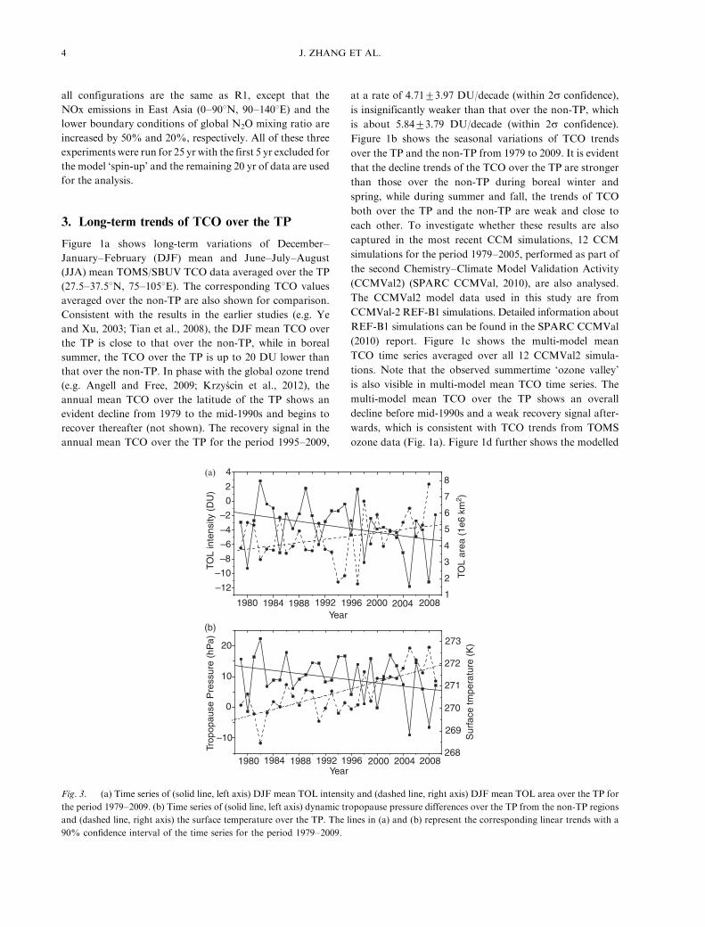
Fig. 3. (a) Time series of (solid line, left axis) DJF mean TOL intensity and (dashed line, right axis) DJF mean TOL area over the TP for
the period 1979�2009. (b) Time series of (solid line, left axis) dynamic tropopause pressure differences over the TP from the non-TP regions
and (dashed line, right axis) the surface temperature over the TP. The lines in (a) and (b) represent the corresponding linear trends with a
90% confidence interval of the time series for the period 1979�2009.
4 J. ZHANG ET AL.
seasonal TCO trends over the TP. The modelled TCO
trends also show a stronger decline over the TP than non-
TP during winter and spring. However, differences between
TCO trends over the TP and non-TP during December and
January are weaker in CCMs simulations than in observa-
tions. The analysis reveals that the modelled warming trend
over the TP during winter, which is an important factor
influencing the TCO trend over the TP as will be discussed
below, is weaker than the observed warming trend (not
shown). This may be one of possible reasons why differ-
ences between TCO trends over the TP and non-TP are
smaller in CCMs simulations than in observations.
Figure 2 shows the decadal variations of TCO anomalies
(defined as the departure of TCO at a given location from
its corresponding zonal mean) for the periods 1980�1989,1990�1999 and 2000�2009. As expected, the summertime
‘ozone valley’ is the most evident. However, there exists
a total column ozone low (TOL) over the TP throughout
a year, that is, the TCO over the TP is always lower than
that over other regions at the same latitude of the TP.
Particularly noticeable is that the TOL is deepening and
the area of TOL is widening during winter and spring for
the period 2000�2009 than before. In contrast, the intensity
and the area of the summertime TOL have no significant
changes during the last three decades. To quantify the
trend of TOL area in winter, the area with DJF mean TCO
anomalies over the TP within the region 20.58N-44.58Nand 708E-1108E lower than �5 DU is counted based on
the high resolution NIWA TCO data. In addition, the area-
weighted average of DJF mean TCO anomalies over the TP
is used as the measure of the TOL intensity. The time series
of wintertime TOL area and intensity are shown in Fig. 3a.
The TOL area exhibits a statistically significant positive
trend of 50,000 km2/decade while the TOL intensity has an
evident negative trend of �1.4 DU/decade, indicating that
the TOL area is widening and deepening. Both of these
trends are statistically significant at 90% confidence level.
It is also noteworthy that 2000�2009 is the period when the
TOL deepens and extends at a more rapid rate than before,
in accordance with Fig. 2.
4. Factors affecting the TOL trend
In this section, we will clarify the factors and processes
responsible for the deepening of the TOL. Figure 3b shows
dynamic tropopause pressure differences between the TP
and non-TP during winter from 1979 to 2009. The dynami-
cal tropopause is defined as the 3.5 potential vorticity unit
(PVU, 1 PVU�10�6 K �m2 �s�1 �kg�1) surface. It is evident
that tropopause pressure differences between the TP and
non-TP exhibit a negative trend, indicating that the winter-
time tropopause height over the TP increases at a larger rate
than that over the non-TP. Previous studies have showed
that tropopause variations have a large impact on the TCO
over the TP and lifting of tropopause height can gives rise
to decreases in TCO (e.g. Varotsos et al., 2004; Tian et al.,
2008). The more significant lifting of the tropopause over
the TP can lead to larger TCO decreases over the TP than
over non-TP. Figure 3b also indicates that the tropopause
pressure differences between the TP and non-TP positively
correlate with the TOL intensity with a statistically signi-
ficant correlation coefficient of 0.75. The lifting of the tropo-
pause height over the TP is closely related to the regional
climate warming over the TP. Previous studies documented
that the TP has warmed most rapidly in the Northern
Hemisphere since the latter half of the 20th century and
the largest warming rates occur during the winter months
(e.g. Qin et al., 2009; Rangwala et al., 2009). Figure 3b
indicates that the surface temperature over the TP exhibits
CRU3 Surface Temperature60N
(a)
(b)
(c)
40N
20N
0
60N
40N
20N
0
60N
40N
20N
0
0 30E 60E 90E 120E150E 180150W120W90W 60W 30W 0
0 30E 60E 90E 120E150E 180150W120W90W 60W 30W 0
0.40.20
–0.2–0.4
2.41.20
–1.2
–2.4
1.61.20.80.40
DU/yr
K/yr
hPa/yr
Longitude (degree)
Latit
ude
(deg
ree)
Latit
ude
(deg
ree)
Latit
ude
(deg
ree)
Longitude (degree)
0 30E 60E 90E 120E150E 180150W120W90W 60W 30W 0Longitude (degree)
Interim Tropopause Pressure
TOMS TCO
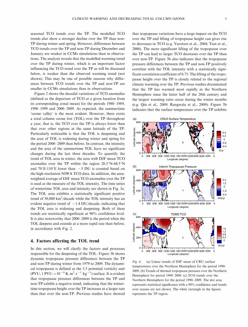
Fig. 4. (a) Linear trends of DJF mean of CRU surface
temperatures over the Northern Hemisphere for the period 1990�2009. (b) Trends of thermal tropopause pressure over the Northern
Hemisphere for period 1990�2009. (c) TCO trends over the
Northern Hemisphere for the period 1990�2009. The dot area
represents statistical significance with a 90% confidence and trends
over oceans are not shown. The white rectangle in the figures
represents the TP region.
CLIMATE WARMING AND DECREASING TOTAL COLUMN OZONE 5
an evident warming trend in winter and this warming trend
becomes more significant during the period 2000�2009.Figure 4a shows trends of DJF mean surface tempera-
tures over the Northern Hemisphere for the period 1990�2009. Note that the TP is one of the regions in the Northern
Hemisphere with a rapid and significant warming trend
during this period, whereas the other regions exhibit rather
weak warming, even significant cooling over the northern
Eurasia and North America, which has also been reported
by Cohen et al. (2012). The DJF mean of thermal tro-
popause pressure for the period 1990�2009 in Fig. 4b
shows a significant negative trend over the TP, indicating
that the tropopause over the TP is rising. Overall, Fig. 4a
and b indicate that the regions with significant surface
warming (cooling) are accompanied by the tropopause
height increases (decreases). Figure 4c shows the linear trends
of DJF mean TCO over the Northern Hemisphere for the
period 1990�2009. Consistent with the results in previous
studies (e.g. Krzyscin et al., 2012), the TCO in the middle
and high latitudes shows significant recovery signals during
this period due to the decline of ODSs, whereas the TCO
in the lower latitude exhibits weaker positive trend and
even negative trend, as an indication of increased tropical
upwelling (Austin et al., 2010). It is particularly noticeable
that the TCO over the TP exhibits a decline trend for the
period 1990�2009, in accordance with the deepening of the
TOL over the recent decade shown in Fig. 3a.
To further verify that the changes in TCO and tropopause
pressure over the TP are both linked to the climate warming
of the TP, a composite analysis is performed with respect to
the DJF mean surface temperatures over the TP. Here, the
warm (cold) composite for a given field is calculated by
averaging the field over the years in which the DJF mean
surface temperature anomaly over the TP (relative to the
1979�2009 mean annual cycle) is greater (less) than 1 (�1)
standard deviation of the time series of the surface tempera-
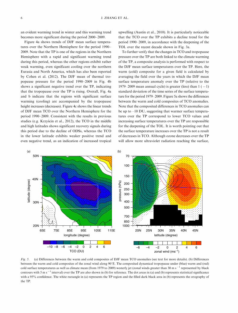
ture for the period 1979�2009. Figure 5a shows the differencesbetween the warm and cold composites of TCO anomalies.
Note that the composited differences in TCO anomalies can
be up to �10 DU, suggesting that warmer surface tempera-
tures over the TP correspond to lower TCO values and
increasing surface temperatures over the TP are responsible
for the deepening of the TOL. It is worth pointing out that
the surface temperature increases over the TP is not a result
of decreases in TCO. Although ozone decreases over the TP
will allow more ultraviolet radiation reaching the surface,
(a) (b)50N 70
100
150
200
250
300
400
500
700
8501000
20N 25N 30N 35N 40N 45N
40N
30N
20N
65E 75E 85E 95E 105E 115E
longitude (degree) latitude (degree)
latit
ude
(deg
ree)
pres
sure
(hP
a)
–10 –8 –6 –4 –2 0 2 4 6 –6zonal wind (ms–1)TCO (DU)
–4 –2 0 2 4 6
Fig. 5. (a) Differences between the warm and cold composites of DJF mean TCO anomalies (see text for more details). (b) Differences
between the warm and cold composites of the zonal wind along 908E. The composited dynamical tropopause under (blue) warm and (red)
cold surface temperatures as well as climate mean (from 1979 to 2009) westerly jet (zonal winds greater than 30 m s�1 represented by black
contours with 5 m s�1 interval) over the TP are also shown in (b) for reference. The dot areas in (a) and (b) represents statistical significance
with a 95% confidence. The white rectangle in (a) represents the TP region and the filled dark black area in (b) represents the orography of
the TP.
6 J. ZHANG ET AL.
this energy change is too small to cause a significant warm-
ing over the TP (Forster and Shine, 1997;McFarlane, 2008).
Rangwala et al. (2009) pointed out that the rapid rising of
the surface temperature over the TP is directly caused by
increasing downward long wave radiation due to increases
in the surface humidity and absorbed solar energy when
snow cover over the TP is reduced.
The wintertime warming can lead to an increase in
the tropopause height over the TP not only through the
expansion of air, but also via changing the jet position in
the subtropics. Figure 5b shows the differences between the
warm and cold composites of the zonal wind along 908E.The composited dynamical tropopause pressures corre-
sponding to warm and cold surface temperatures are also
overplotted for reference. It is apparent that the dynamic
tropopause height under anomalously warm surface tem-
peratures over the TP is higher than that under anomalously
cold surface temperatures. The zonal wind differences be-
tween its warm and cold composites show significant posi-
tive anomalies to the north of the TP and negative anomalies
to the south of the TP in the upper troposphere. Compared
to the climatological mean position of the westerly jet shown
in Fig. 5b, these zonal wind anomalies suggest a poleward
shift of the westerly jet under anomalously high tempera-
tures over the TP, which should also contribute to the
increases in the tropopause height over the TP (e.g. Liu et al.,
2010; Fu and Lin, 2011).
Tian et al. (2008) argued that lifting of the tropopause
height over the TP tends to cause an overall upward shift of
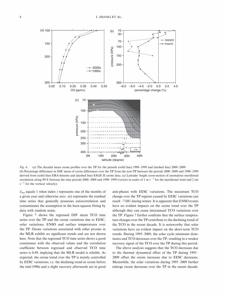
ozone profiles, and hence reduced TCO values. Figure 6a
shows the decadal mean ozone profiles over the TP for the
periods 1990�1999 and 2000�2009. In the upper tropo-
sphere and lower stratosphere (UTLS), the mean ozone
profile during the 2000s indeed shifts upward relative to
that during the 1990s. Meanwhile, both ERA-Interim and
SAGE II ozone data indicates that the negative differences
of ozone mixing ratios in the UTLS over the TP from the
non-TP for the time period 2000�2009 are stronger than
those for the time period 1990�1999 (Fig. 6b). It can be
estimated from the ERA-Interim ozone data that the larger
ozone decreases between 200 hPa and 70 hPa over the TP
relative to those over the non-TP in the recent decade have
a 55% contribution to the deepening of the TOL.
Another factor that is likely to affect the TCO over the TP
is the transport process. Austin et al. (2010) pointed out that
strengthening Brewer-Dobson (BD) circulation in a warm-
ing climate can lead to ozone decreases in tropical lower
stratosphere as a result of intensified upward transport
of ozone-poor air from below. On the contrary, previous
studies have shown convincing evidence that the Hadley
circulation is strengthening in recent years (Mitas and
Clement, 2005; Hu et al., 2011); consequently, the meridio-
nal transport of air mass tends to be enhanced in the UTLS
at lower latitudes. Figure 6c shows meridional circulation
changes between the time periods 2000�2009 and 1990�1999. The anomalous circulation shows that the meridional
transport of ozone poor air in the tropical upper tropo-
sphere towards the subtropical lower stratosphere is
enhanced in the 2000s and this feature is particularly
pronounced above 300 hPa in subtropical UTLS. The above
analysis indicate that the TCO decreases over the TP in
the recent decade result mainly from the combined effect
of rising tropopause and enhanced meridional transport of
air masses.
To further clarify the relative importance of different
factors in modulating the interannual variations of TCO
over the TP, the multiple regression model (MLR) ana-
lysis is applied on the TCO time series from 1979 to 2009.
The MLR is a useful tool to attribute ozone variations
to dynamical, radiative and chemical effects (e.g. SPARC
CCMVal, 2010;WMO, 2011). The proxy variables used here
are similar to those in Dhomse et al. (2006) with the surface
temperature over the TP as an additional proxy variable.
The MLR can be represented as follows:
TCOðtÞ ¼X12
m¼1
a0m � dmn þ
X12
m¼1
aEESCm � dmn � EESCðtÞ
þX12
m¼1
aQBO10m � dmn �QBO10ðtÞ
þX12
m¼1
aQBO30m � dmn �QBO30ðtÞ
þX12
m¼1
aaerom � dmn � aeroðtÞ
þX12
m¼1
asolarm � dmn � solarðtÞ
þX12
m¼1
aENSOm � dmn � ENSOðtÞ
þX12
m¼1
aEPfluxm � dmn � EPfluxðtÞ
þX12
m¼1
atsm � dmn � tsðtÞ þ eðtÞ
where t is the time in 1-month increments. a0m (m�1,. . .,12)
is the long-term mean for the mth month of the year.
axm is the contribution coefficient of proxy x. The proxies
selected for the MLR model include the equivalent effective
stratospheric chlorine (EESC), the Quasi-biennial oscilla-
tion (QBO) index at 10 and 30 hPa measured at Singapore
(QBO10 and QBO30), the stratospheric aerosol 550 nm
optical depths (aero), the solar cycle effect represented
by F10.7 solar flux (solar), Nino3 ENSO Index (ENSO),
the horizontal EP flux at 100 hPa over the 458N to 758N(EPflux), and the surface temperature over the TP (Ts).
CLIMATE WARMING AND DECREASING TOTAL COLUMN OZONE 7
dmn equals 1 when index t represents one of the months of
a given year and otherwise zero. o(t) represents the residual
time series that generally possesses autocorrelation and
contaminates the assumption in the least-squares fitting by
data with random noise.
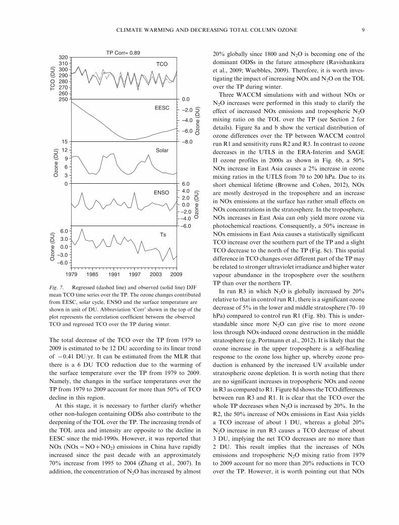
Figure 7 shows the regressed DJF mean TCO time
series over the TP and the ozone variations due to EESC,
solar variations, ENSO and surface temperatures over
the TP. Ozone variations associated with other proxies in
the MLR exhibit no significant trends and are not shown
here. Note that the regressed TCO time series shows a good
consistence with the observed values and the correlation
coefficient between regressed and observed TCO time
series is 0.89, implying that the MLR model is reliable. As
expected, the ozone trend over the TP is mainly controlled
by EESC variations, i.e. the declining trend in ozone before
the mid-1990s and a slight recovery afterwards are in good
anti-phases with EESC variations. The maximum TCO
change over the TP regions caused by EESC variations can
reach �7 DU during winter. It is apparent that ENSO events
have no evident impacts on the ozone trend over the TP
although they can cause interannual TCO variations over
the TP. Figure 7 further confirms that the surface tempera-
ture changes over the TP contribute to the declining trend of
the TCO in the recent decade. It is noteworthy that solar
variations have an evident impact on the short-term TCO
trends. During 1995�2009, the solar cycle minimum dom-
inates and TCO decreases over the TP, resulting in a weaker
recovery signal of the TCO over the TP during this period.
The above analysis suggests that the TCO decreases due
to the thermal�dynamical effect of the TP during 1995�2009 offset the ozone increases due to EESC decreases.
Meanwhile, the solar variations during 1995�2009 further
enlarge ozone decreases over the TP in the recent decade.
100
150
(a)
(c)
(b) 1030
70
100
150
200
300
200
2000s
SAGEIIInterim
1990s
3000.00 0.10 0.20
O3 (ppmv)
70
100
150
200
pres
sure
(hP
a)
pres
sure
(hP
a)
250
300
4000N 10N 20N 30N 40N
0.30 0.40 0.50 –8.0 –6.0 –4.0percentage change (%)
latitude (degree)
–2.0 0.0 2.0 4.0
Fig. 6. (a) The decadal mean ozone profiles over the TP for the periods (solid line) 1990�1999 and (dashed line) 2000�2009.(b) Percentage differences in DJF mean of ozone differences over the TP from the non-TP between the periods 2000�2009 and 1990�1999derived from (solid line) ERA-Interim and (dashed line) SAGE II ozone data. (c) Latitude�height cross-section of anomalous meridional
circulation along 908E between the time periods 2000�2009 and 1990�1999 (vectors in scales of 1 m s�1 for the meridional wind and 2 cm
s�1 for the vertical velocity).
8 J. ZHANG ET AL.
The total decrease of the TCO over the TP from 1979 to
2009 is estimated to be 12 DU according to its linear trend
of �0.41 DU/yr. It can be estimated from the MLR that
there is a 6 DU TCO reduction due to the warming of
the surface temperature over the TP from 1979 to 2009.
Namely, the changes in the surface temperatures over the
TP from 1979 to 2009 account for more than 50% of TCO
decline in this region.
At this stage, it is necessary to further clarify whether
other non-halogen containing ODSs also contribute to the
deepening of the TOL over the TP. The increasing trends of
the TOL area and intensity are opposite to the decline in
EESC since the mid-1990s. However, it was reported that
NOx (NOx�NO�NO2) emissions in China have rapidly
increased since the past decade with an approximately
70% increase from 1995 to 2004 (Zhang et al., 2007). In
addition, the concentration of N2O has increased by almost
20% globally since 1800 and N2O is becoming one of the
dominant ODSs in the future atmosphere (Ravishankara
et al., 2009; Wuebbles, 2009). Therefore, it is worth inves-
tigating the impact of increasing NOx and N2O on the TOL
over the TP during winter.
Three WACCM simulations with and without NOx or
N2O increases were performed in this study to clarify the
effect of increased NOx emissions and tropospheric N2O
mixing ratio on the TOL over the TP (see Section 2 for
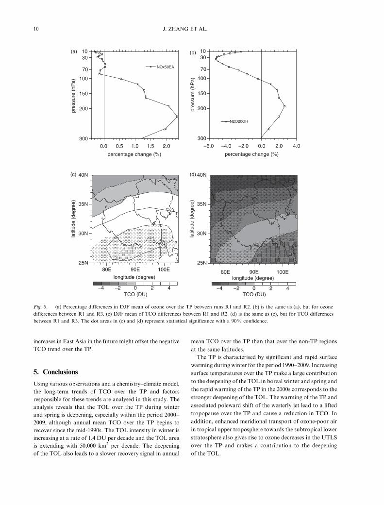
details). Figure 8a and b show the vertical distribution of
ozone differences over the TP between WACCM control
run R1 and sensitivity runs R2 and R3. In contrast to ozone
decreases in the UTLS in the ERA-Interim and SAGE
II ozone profiles in 2000s as shown in Fig. 6b, a 50%
NOx increase in East Asia causes a 2% increase in ozone
mixing ratios in the UTLS from 70 to 200 hPa. Due to its
short chemical lifetime (Browne and Cohen, 2012), NOx
are mostly destroyed in the troposphere and an increase
in NOx emissions at the surface has rather small effects on
NOx concentrations in the stratosphere. In the troposphere,
NOx increases in East Asia can only yield more ozone via
photochemical reactions. Consequently, a 50% increase in
NOx emissions in East Asia causes a statistically significant
TCO increase over the southern part of the TP and a slight
TCO decrease to the north of the TP (Fig. 8c). This spatial
difference in TCO changes over different part of the TP may
be related to stronger ultraviolet irradiance and higher water
vapour abundance in the troposphere over the southern
TP than over the northern TP.
In run R3 in which N2O is globally increased by 20%
relative to that in control run R1, there is a significant ozone
decrease of 5% in the lower and middle stratosphere (70�10hPa) compared to control run R1 (Fig. 8b). This is under-
standable since more N2O can give rise to more ozone
loss through NOx-induced ozone destruction in the middle
stratosphere (e.g. Portmann et al., 2012). It is likely that the
ozone increase in the upper troposphere is a self-healing
response to the ozone loss higher up, whereby ozone pro-
duction is enhanced by the increased UV available under
stratospheric ozone depletion. It is worth noting that there
are no significant increases in tropospheric NOx and ozone
inR3as compared toR1.Figure 8d shows theTCOdifferences
between run R3 and R1. It is clear that the TCO over the
whole TP decreases when N2O is increased by 20%. In the
R2, the 50% increase of NOx emissions in East Asia yields
a TCO increase of about 1 DU, whereas a global 20%
N2O increase in run R3 causes a TCO decrease of about
3 DU, implying the net TCO decreases are no more than
2 DU. This result implies that the increases of NOx
emissions and tropospheric N2O mixing ratio from 1979
to 2009 account for no more than 20% reductions in TCO
over the TP. However, it is worth pointing out that NOx
320TP Corr= 0.89
TCO
EESC
Solar
0.0
6.04.02.00.0–2.0–4.0–6.0
–2.0
–4.0
–6.0
–8.0
ENSO
Ts
310300290280270260250
15
12
9
6
3
0
6.0
3.0
0.0
–3.0
Ozo
ne (
DU
)O
zone
(D
U)
Ozo
ne (
DU
)O
zone
(D
U)
TC
O (
DU
)
–6.0
1979 1985 1991 1997 2003 2009
Fig. 7. Regressed (dashed line) and observed (solid line) DJF
mean TCO time series over the TP. The ozone changes contributed
from EESC, solar cycle, ENSO and the surface temperature are
shown in unit of DU. Abbreviation ‘Corr’ shown in the top of the
plot represents the correlation coefficient between the observed
TCO and regressed TCO over the TP during winter.
CLIMATE WARMING AND DECREASING TOTAL COLUMN OZONE 9
increases in East Asia in the future might offset the negative
TCO trend over the TP.
5. Conclusions
Using various observations and a chemistry�climate model,
the long-term trends of TCO over the TP and factors
responsible for these trends are analysed in this study. The
analysis reveals that the TOL over the TP during winter
and spring is deepening, especially within the period 2000�2009, although annual mean TCO over the TP begins to
recover since the mid-1990s. The TOL intensity in winter is
increasing at a rate of 1.4 DU per decade and the TOL area
is extending with 50,000 km2 per decade. The deepening
of the TOL also leads to a slower recovery signal in annual
mean TCO over the TP than that over the non-TP regions
at the same latitudes.
The TP is characterised by significant and rapid surface
warming during winter for the period 1990�2009. Increasingsurface temperatures over the TP make a large contribution
to the deepening of the TOL in boreal winter and spring and
the rapid warming of the TP in the 2000s corresponds to the
stronger deepening of the TOL. The warming of the TP and
associated poleward shift of the westerly jet lead to a lifted
tropopause over the TP and cause a reduction in TCO. In
addition, enhanced meridional transport of ozone-poor air
in tropical upper troposphere towards the subtropical lower
stratosphere also gives rise to ozone decreases in the UTLS
over the TP and makes a contribution to the deepening
of the TOL.
(a)
(c) (d)
(b)1030
NOx50EA
N2O20GH
70
100
150
pres
sure
(hP
a)
pres
sure
(hP
a)
200
300
40N
35N
30N
25N80E
–4 –2 0 2 4
90E 100E
TCO (DU)–4 –2 0 2 4
TCO (DU)
80E 90E 100E
1030
70
100
150
200
300
0.0 0.5
percentage change (%)
longitude (degree)
latit
ude
(deg
ree)
40N
35N
30N
25N
latit
ude
(deg
ree)
longitude (degree)
percentage change (%)
1.0 1.5 2.0 –6.0 –4.0 –2.0 0.0 2.0 4.0
Fig. 8. (a) Percentage differences in DJF mean of ozone over the TP between runs R1 and R2. (b) is the same as (a), but for ozone
differences between R1 and R3. (c) DJF mean of TCO differences between R1 and R2. (d) is the same as (c), but for TCO differences
between R1 and R3. The dot areas in (c) and (d) represent statistical significance with a 90% confidence.
10 J. ZHANG ET AL.
Based on the MLR analysis, the TCO trends over TP
are mainly controlled by EESC and are evidently affected
by the surface warming of the TP and solar variations. The
ozone reductions due to rising surface temperature cause
a weaker recovery signal of TCO over the TP in the recent
decade compared to that over the non-TP, while solar cycle
minimum makes the ozone recovery signal even weaker
after mid-1990s. Rising surface temperatures over the TP
for the period 1979�2009 account for up to 50% of TCO
decline over the TP, while increases in NOx emissions
and tropospheric N2O contribute to no more than 20%
reductions in TCO for the period 1979�2009.The deepening of the TOL makes the recovery of TCO
over the TP less significant than that over the non-TP
regions of the same latitudes. Rangwala et al. (2010) have
shown that the surface temperature over the TP during
winter and spring will continue to rise at a rapid rate during
the 21st century under the SRES A1B scenario. Therefore,
the TOL over the TP during winter and spring is likely to
deepen and extend continuously. In addition, the increas-
ing global tropospheric N2O in the future might further
deepen the TOL over the TP. However, for the foreseeable
future, the impact of global warming/loss of snow over the
TP on the TOL will be mitigated by decreasing chlorine and
bromine loading in the stratosphere and NOx emissions
increases in East Asia.
6. Acknowledgements
This work is supported by the National Science Foundation
of China (41175042, 41225018) J. Luo is supported by the
Scholarship Award for Excellent Doctoral Student granted
by Lanzhou University. The authors thank the scientific
teams NASA, ECMWF, CRU and China Meteorological
Administration for providing data. Dr.GregBodeker kindly
provided the NIWA TCO data. Comments and suggestions
from the anonymous reviewers and the editor were valu-
able in improving the quality of this paper. The authors
also thank Dr. Eri Saikawa, Prof. Aijun Ding and Dr. Dong
Guo for their helpful suggestions. Finally, the authors
acknowledged the computing support provided by the
Supercomputing Center of Cold and Arid Regions Environ-
mental and Engineering Research Institute of Chinese
Academy of Sciences.
References
Angell, J. K. and Free, M. 2009. Ground-based observations of
the slowdown in ozone decline and onset of ozone increase.
J. Geophys. Res. 114, D07303, 1�9.Austin, J., Scinocca, J., Plummer, D., Oman, L., Waugh, D. and
co-authors. 2010. Decline and recovery of total column ozone
using a multimodel time series analysis. J. Geophys. Res. 115,
D00M10.
Bodeker, G. E., Shiona, H. and Eskes, H. 2005. Indicators of
Antarctic ozone depletion. Atmos. Chem. Phys. 5, 2603�2615.Browne, E. C. and Cohen, R. C. 2012. Effects of biogenic nitrate
chemistry on the NOx lifetime in remote continental regions.
Atmos. Chem. Phys. 12, 11917�11932.Cohen, J. L., Furtado, J. C., Barlow, M., Alexeev, V. A. and
Cherry, J. E. 2012. Asymmetric seasonal temperature trends.
Geophys. Res. Lett. 39, L04705.
Dhomse, S., Weber, M., Wohltmann, I., Rex, M. and Burrows,
J. P. 2006. On the possible causes of recent increases in northern
hemispheric total ozone from a statistical analysis of satellite
data from 1979 to 2003. Atmos. Chem. Phys. 6, 1165�1180.Dragani, R. 2011. On the quality of the ERA-Interim ozone
reanalyses: comparisons with satellite data. Q. J. R. Meteorol.
Soc. 137, 1312�1326.Forster, P. M. d. F. and Shine, K. P. 1997. Radiative forcing
and temperature trends from stratospheric ozone changes.
J. Geophys. Res. 102, 10841�10855.Fu, Q. and Lin, P. 2011. Poleward shift of subtropical jets inferred
from satellite-observed lower-stratospheric temperatures. J. Clim.
24, 5597�5603.Garcia, R. R., Marsh, D. R., Kinnison, D. E., Boville, B. A. and
Sassi, F. 2007. Simulation of secular trends in the middle
atmosphere, 1950�2003. J. Geophys. Res. 112, D09301.
Horowitz, L. W., Walters, S., Mauzerall, D. L., Emmons, L. K.,
Rasch, P. J. and co-authors. 2003. A global simulation of
tropospheric ozone and related tracers: description and eval-
uation of MOZART, version 2. J. Geophys. Res. 108(D24),
4784.
Hu, Y. Y., Zhou, C. and Liu, J. P. 2011. Observational evidence
for the poleward expansion of the Hadley circulation. Adv.
Atmos. Sci. 28(1), 33�44.Krzyscin, J. W. 2012. Onset of the total ozone increase based on
statistical analyses of global ground-based data for the period
1964�2008. Int. J. Climatol 32, 240�246.Liu, C. X., Liu, Y., Cai, Z. N., Gao, S. T., Bian, J. C. and
co-authors. 2010. Dynamic formation of extreme ozone mini-
mum events over the Tibetan Plateau during northern winters
1987�2001. J. Geophys. Res. 115, D18311.
Liu, Y., Li, W. L. and Zhou, X. J. 2001. Prediction of the trend of
total column ozone over the Tibetan Plateau. Science in China.
44(Suppl), 385�389 (in Chinese).
McFarlane, N. 2008. Connections between stratospheric ozone
and climate: radiative forcing, climate variability, and change.
Atmos. Ocean 46, 139�158.Mitas, C. M. and Clement, A. 2005. Has the Hadley cell been
strengthening in recent decades? Geophys. Res. Lett. 32, L03809.
Portmann, R. W., Daniel, J. S. and Ravishankara, A. R. 2012.
Stratospheric ozone depletion due to nitrous oxide: influences
of other gases. Phil. Trans. R. Soc. B. 367, 1256�1264.Qin, J., Yang, K., Liang, S. L. and Guo, X. F. 2009. The
altitudinal dependence of recent rapid warming over the Tibetan
Plateau. Clim. Change. 97, 321�327.Rangwala, I., Miller, J. R., Russell, G. L. and Xu, M. 2010.
Using a global climate model to evaluate the influences of water
CLIMATE WARMING AND DECREASING TOTAL COLUMN OZONE 11
vapour, snow cover and atmospheric aerosol on warming in the
Tibetan Plateau during the twenty-first century. Clim. Dyn. 34,
859�872.Rangwala, I., Miller, J. R. and Xu, M. 2009. Warming in the
Tibetan Plateau: possible influences of the changes in surface
water vapor. Geophys. Res. Lett. 36, L06703.
Ravishankara, A. R., Daniel, J. S. and Portmann, R. W. 2009.
Nitrous oxide (N2O): the dominant ozone-depleting substance
emitted in the 21st century. Science. 326, 123�125.Skerlak, B., Sprenger, M. and Wernli, H. 2013. A global clima-
tology of stratosphere-troposphere exchange using the ERA-
interim dataset from 1979 to 2011. Atmos. Chem. Phys. Discuss.
13, 11537�11595.SPARC CCMVal. 2010. SPARC Report on the Evaluation
of Chemistry�Climate Models. V. Eyring, T. G. Shepherd,
D. W. Waugh (Eds.), SPARC Report No. 5, WCRP-132,
WMO/TD-No. 1526.
Tian, W. S., Chipperfield, M. P. and Huang, Q. 2008. Effects of
the Tibetan Plateau on total column ozone distribution. Tellus
B. 60, 622�635.Tobo, Y., Iwasaka, Y., Zhang, D. Z., Shi, G. Y., Kim, Y. S. and
co-authors. 2008. Summertime ‘ozone valley’ over the Tibetan
Plateau derived from ozonesondes and EP/TOMS data. Geophys.
Res. Lett. 35, L16801.
Varotsos, C., Cartalis, C., Vlamakis, A., Tzanis, C. and
Keramitsoglou, I. 2004. The long-term coupling between column
ozone and tropopause properties. J. Clim. 17, 3843�3854.
World Meteorological Organization (WMO). 2011. Scientific Assess-
ment of Ozone Depletion: 2010. Global Ozone Research and
Monitoring Project-Report No. 52, WMO, Geneva, Switzerland.
Wuebbles, D. J. 2009. Nitrous oxide: no laughing matter. Science.
326(5949), 56�57.Yanai, M., Li, C. F. and Song, Z. S. 1992. Seasonal heating of the
Tibetan Plateau and its effects on the evolution of the Asian
summer monsoon. J. Meteorol. Soc. Jpn. 70, 319�351.Ye, D. Z. and Wu, G. X. 1998. The role of the heat source of the
Tibetan Plateau in the general circulation. Meteorol. Atmos.
Phys. 67, 181�198.Ye, Z. J. and Xu, Y. F. 2003. Climate characteristics of ozone over
Tibetan Plateau. J. Geophys. Res. 108(D20), 4654.
Zhang, Q., Streets, D. G., He, K. B., Wang, Y. X., Richter, A. and
co-authors. 2007. NOx emissions trends for China, 1995�2004:the view from the ground and the view from space. J. Geophys.
Res. 112, D22306.
Zheng, X. D., Zhou, X. J., Tang, J., Qin, Y. and Chan, C. Y. 2004.
A meteorological analysis on a low tropospheric ozone event
over Xining, North Western China on 26�27 July 1996. Atmos.
Environ. 38, 261�271.Zhou, X. J., Luo, C., Li, W. L. and Shi, J. E. 1995. Ozone changes
over China and low center over Tibetan Plateau. Chin. Sci. Bull.
40, 1396�1398 (in Chinese).
Zou, H. 1996. Seasonal variation and trends of TOMS ozone over
Tibet. Geophys. Res. Lett. 23(9), 1029�1032.
12 J. ZHANG ET AL.

Copyright of Tellus: Series B is the property of Co-Action Publishing and its content may notbe copied or emailed to multiple sites or posted to a listserv without the copyright holder'sexpress written permission. However, users may print, download, or email articles forindividual use.
Recommended