
1 | P a g e
Classification of Caesarean Section and Normal Vaginal
Deliveries Using Foetal Heart Rate Signals and Advanced
Machine Learning Algorithms
Paul Fergus1, Abir Hussain
1, Dhiya Al-Jumeily
1 De-Shuang Huang
2, Nizar Bouguila
3
1Applied Computing Research Group,
Faculty of Engineering and Technology,
Department of Computer Science,
Liverpool John Moors University,
Byron Street,
Liverpool,
L3 3AF,
United Kingdom.
Email: [email protected] (Paul Fergus)
Tel: (+44) 151 231 2629
Email: [email protected] (Abir Hussain)
Tel: (+44) 151 231 2458
Email: [email protected] (Dhiya Al-Jumeily)
Tel: (+44) 151 231 2578
2Institute of Machine Learning and Systems Biology,
Tongji University,
No. 4800 Caoan Road,
Shanghai,
201804,
China.
Email: [email protected]
Tel: (+86) 021 33514140
3Concordia Institute for Information Systems Engineering,
Concorida University,
1455 de Maisonneuve Blvd West,
EV7.632,
Montreal,
Quebec,
HJ3G 2W1,
Canada.
Email: [email protected]
Tel: 514-848 2424 ext. 5663

2 | P a g e
Classification of Caesarean Section and Normal Vaginal
Deliveries Using Foetal Heart Rate Signals and
Advanced Machine Learning Algorithms
ABSTRACT – Background: Visual inspection of Cardiotocography traces by
obstetricians and midwives is the gold standard for monitoring the wellbeing of the
foetus during antenatal care. However, inter- and intra-observer variability is high
with only a 30% positive predictive value for the classification of pathological
outcomes. This has a significant negative impact on the perinatal foetus and often
results in cardio-pulmonary arrest, brain and vital organ damage, cerebral palsy,
hearing, visual and cognitive defects and in severe cases, death. This paper shows
that using machine learning and foetal heart rate signals provides direct information
about the foetal state and helps to filter the subjective opinions of medical
practitioners when used as a decision support tool. The primary aim is to provide a
proof-of-concept that demonstrates how machine learning can be used to objectively
determine when medical intervention, such as caesarean section, is required and
help avoid preventable perinatal deaths. Methodology: This is evidenced using an
open dataset that comprises 506 controls (normal virginal deliveries) and 46 cases
(caesarean due to pH ≤7.05 and pathological risk). Several machine-learning
algorithms are trained, and validated, using binary classifier performance measures.
Results: The findings show that deep learning classification achieves Sensitivity =
94%, Specificity = 91%, Area under the Curve = 99%, F-Score = 100%, and Mean
Square Error = 1%. Conclusions: The results demonstrate that machine learning
significantly improves the efficiency for the detection of caesarean section and
normal vaginal deliveries using foetal heart rate signals compared with obstetrician
and midwife predictions and systems reported in previous studies.
Keywords: Classification, Feature Extraction and Selection, Deep Learning,
Intrapartum Cardiotocography, Machine Learning, Random Forest.
1. INTRODUCTION

3 | P a g e
Worldwide, over 130 million babies are born each year. 3.6 million will die due to
perinatal complication and 1 million of these will be intrapartum still births [1]. In the
USA, the number of deliveries in 2012 was 3,952,841; one in every 164 of these
resulted in stillbirth1. In the UK, in the same year, there were 671,255 with one in
every 200 being stillbirth2 and 300 that died in the first four weeks of life [2].
Cardiotocography (CTG) is the most common method used to monitor the foetus
during the early stages of delivery [3] and clinical decisions are made using the
visual inspection of CTG traces. However, the main weakness with this approach is
poor human interpretation which leads to high inter- and intra-observer variability [4].
While significant pathological outcomes like hypoxia are uncommon, false alarms are
not, which can lead to serious abnormalities, such as cardio-pulmonary arrest, brain
and vital organ damage, cerebral palsy, hearing, visual and cognitive defects and in
severe cases, death, being overlooked [5]. Conversely, over interpretation of CTG is
common and the direct cause of unnecessary caesarean sections (CS). In such
cases, between 40 and 60 percent of babies are born without any evidence to
support pathological outcomes, such as hypoxia and metabolic acidosis [6].
This paper aims to address this problem by incorporating a proof-of-concept
system alongside existing gold standard methods in antenatal care. Using foetal
heart rate signals and machine learning an objective measure of foetal state is used
to detect the onset of pathological cases. This will provide obstetricians and
midwives with an additional level of foetal state interpretation and help decide if and
when surgical intervention is required. The results show that the approach has
superior predictive capacity when compared with the 30% positive predictive value
produced by obstetricians and midwives when classifying normal vaginal and
caesarean section deliveries [15].
The remainder of this paper is organized as follows. Section 2 provides
background and related work and Section 3 describes the materials and methods
used in this paper. Section 4 presents the results and the findings are discussed in
Section 5. The paper is concluded in Section 6.
2. BACKGROUND
1 http://www.cdc.gov/
2 http://www.hscic.gov.uk

4 | P a g e
CTG was initially developed as a screening tool to predict foetal hypoxia [15].
However, there is no evidence to suggest that there has been any improvement in
perinatal deaths since the introduction of CTG into clinical practice 45 years ago. It is
generally agreed that 50% of birth-related brain injuries are preventable, with
incorrect CTG interpretation leading the list of causes [12]. Equally, over
interpretation of CTG is common and the direct cause of unnecessary caesarean
sections, which costs the NHS £1,700 for each caesarean performed compared with
£750 for a normal vaginal delivery. It is therefore generally agreed that predicting
adverse pathological outcomes and diagnosing pathological outcomes earlier clearly
have important consequences, for both health and the economy. One interesting
approach is machine learning.
Warrick et al. [15] developed a system for the classification of normal and hypoxic
foetuses by modelling the FHR and Uterine Contraction (UC) signal pairs as an
input-output system to estimate their dynamic relation in terms of an impulse
response function [17]. The authors report that their system can detect almost half of
the pathological cases 1 hour and 40 minutes prior to delivery with a 7.5% false
positive rate. Kessler et al. [54] on the other hand, using 6010 high risk deliveries,
combined CTG with ST waveform to apply timely intervention for caesarean or
vaginal delivery, which they report, reduced foetal morbidity and mortality [8].
In comparative studies, Huang et al. [18] compared three different classifiers; a
Decision Tree (DT), an Artificial Neural Network (ANN), and Discriminant Analysis
(DA). Using the ANN classifier, it was possible to obtain a 97.78% overall accuracy.
This was followed by the DT and DA with 86.36% and 82.1% accuracy respectively.
The Sensitivity and Specificity values were not provided making accuracy alone an
insufficient performance measure for binary classifiers. This is particularly true in
evaluations where datasets are skewed in favour of one class with significant
differences between prior probabilities.
In a similar study, Ocak et al. [19] evaluated an SVM and Genetic Algorithm (GA)
classifier and reported 99.3% and 100% accuracies for normal and pathological
cases respectively. Similar results were reported in [20] and [21]. Again, Sensitivity
and Specificity values where not provided in these studies. Meanwhile Menai et al.
[22] carried out a study to classify foetal state using a Naive Bayes (NB) classifier
5 | P a g e
with four different feature selection (FS) techniques: Mutual Information, Correlation-
based, ReliefF, and Information Gain. The study found that the NB classifier in
conjunction with features produced using the ReliefF technique produce the best
results when classifying foetal state with 93.97%, 91.58%, and 95.79% for Accuracy,
Sensitivity and Specificity, respectively. While the results are high, the dataset is
multivariate and highly imbalanced. Alternative model evaluation metrics for multi-
class data, such as micro- and macro-averaging, and micro and macro-F-Measure,
would provide a more informed account of model performance. Furthermore, an
appropriate account of how the class skew problem was addressed is missing.
The adaptive boosting (AdaBoost) classifier was adopted in a study by Karabulut
et al. [23] who report an accuracy of 95.01% - again no Sensitivity or Specificity
values were provided. While Spilka et al., who are the current forerunners of
pioneering work in machine learning and CTG classification [6], used a Random
Forest (RF) classifier in conjunction with latent class analysis (LCA) [24] and
reported Sensitivity and Specificity values of 72% and 78% respectively using the
CTG-UHB dataset [3]. Producing slightly better results in [25] using the same
dataset, Spilka et al. attempted to detect hypoxia using a C4.5 decision tree, Naive
Bayes, and SVM. The SVM produced the best results using a 10-fold cross
validation method achieving 73.4% for Sensitivity and 76.3% of Specificity.
3. MATERIALS AND METHODS
This section describes the dataset adopted in this study and discusses the steps
taken to pre-process the data and extract the features from raw FHR signals. The
section is then concluded with a discussion on the feature selection technique and
dimensionality reduction.
3.1 CTG Data Collection
Chudacek et al. [3] conducted a comprehensive study that captured intrapartum
recordings between April 2010 and August 2012. The recordings were collected from
the University Hospital in Brno (UHB), in the Czech Republic by obstetricians with
the support of the Czech Technical University (CTU) in Prague. These records are
publically available from the CTU-UHB database, in Physionet [3].
6 | P a g e
The CTU-UHB database contains 552 CTG recordings for singleton pregnancies
with a gestational age less than 36 weeks that were selected from 9164 recordings.
The STAN S21/S31 and Avalon FM 40/50 foetal monitors were used to acquire the
CTG records. The dataset contains no prior known development factors (i.e. they are
ordinary clean obstetrics cases); the duration of stage two labour is less than or
equal to 30 minutes; foetal heart rate signal quality is greater than 50 percent in each
30 minutes’ window; and the pH umbilical arterial blood sample is available. In the
dataset, 46 caesarean section deliveries are included and the rest are ordinary clean
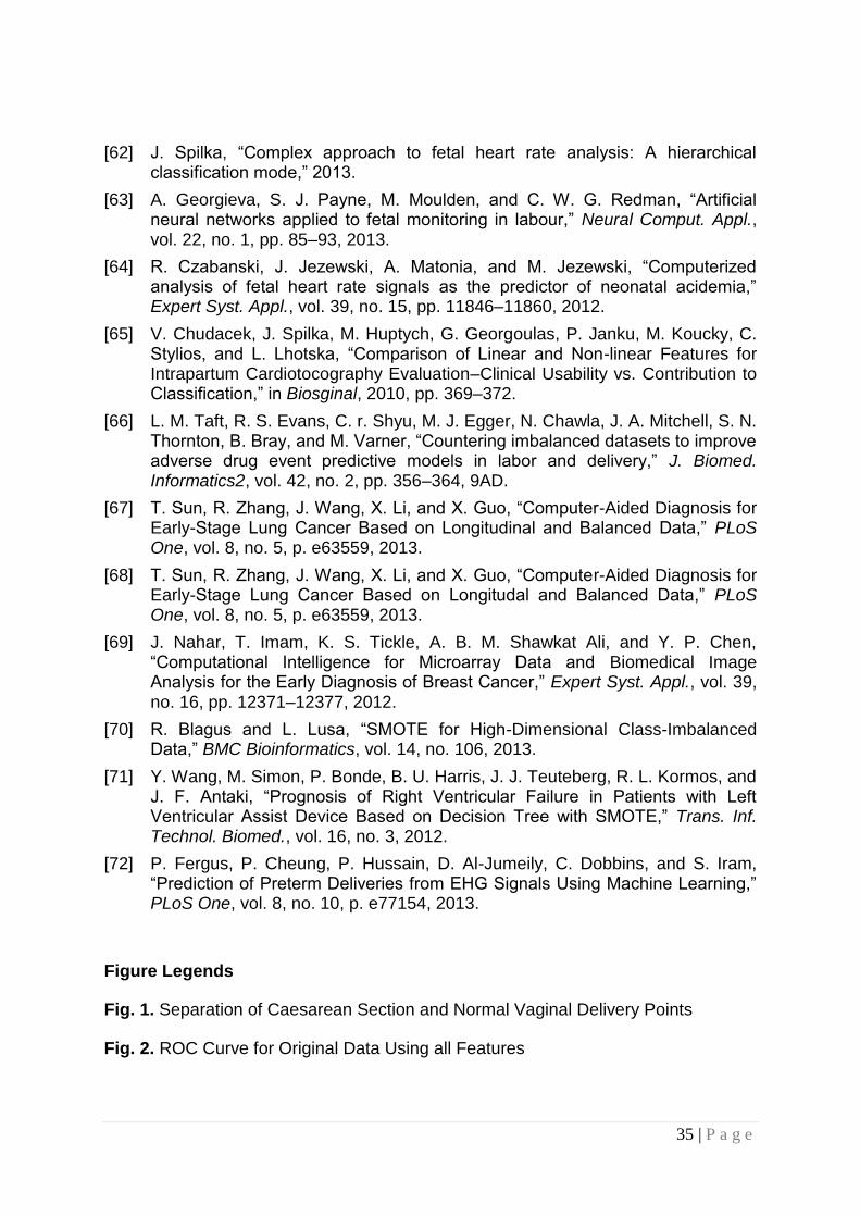
vaginal deliveries. Figure 1 shows a scatter plot of the dataset with eclipses defining
the separation between both case and control groups. Note that in this study a pH
less than or equal to 7.05 is used to classify 16 of the CS records – the remaining 30
are CS records with normal outcomes
Each recording begins no more than 90 minutes before delivery. Each CTG record
contains the FHR time series (measured in beats per minute) and uterine contraction
(UC) signal – each sampled at 4Hz. The FHR was obtained from an ultrasound
transducer attached to the abdominal wall. In this study only the FHR signal is only
considered in this study since it provides direct information about the foetal state.
3.2 Pre-processing
Each of the 552 FHR signal recordings were filtered using a 6th order low-pass
Butterworth filter with fc = 4Hz and a cut-off frequency of 0.034Hz. To correct the
phase distortion introduced by a one-pass filter, a two-pass filter (forwards and
reverse) was used to filter each of the signals. Noise, and missing values were
removed using cubic Hermite spline interpolation [26].
3.3 FHR Features
This section describes the statistical, higher-order statistical and higher-order
spectral features extracted from the FHR signals.
3.3.1 Morphological Features

7 | P a g e
The initial set of features considered are those defined by the International
Federation of Gynecology and Obstetrics3 (FIGO) and the National Institute for
Health and Care Excellence4 (NICE). Consider a raw FHR time series signal X with
length N, where X = {xn, n =1, 2…, N}, in which the Virtual Baseline Mean (VBM), �̄� is
defined as:
x̄ =∑ 𝑥𝑛
𝑁𝑛=1
N
(1)
Such that x̅ can be used to remove accelerations and decelerations (𝑖𝑓 𝑥𝑛 > 10 + x̅
𝑡ℎ𝑒𝑛: 𝑥𝑛 = x̄ + 10; 𝑖𝑓 𝑥𝑛 < −10 + x̅ 𝑡ℎ𝑒𝑛: 𝑥𝑛 = x̄ + −10) from the FHR signal so
that the real baseline FHR (RBL) can be derived [27]:
RBL =∫ X
H
L
N
(2)
Where H and L are the upper and lower limits of the time series signal respectively,
X is the signal and N is the length of the signal.
Using the RBL, FIGO accelerations and decelerations can be extracted. These are
features commonly used by obstetricians to monitor the interplay between the
sympathetic and parasympathetic systems. Accelerations and decelerations within X
represent the transient increases and decreases (±15bpm) that last for 15s or more
[28]. In the case of accelerations, this typically indicates adequate blood delivery and
is reassuring for the obstetrician. Calculating accelerations in the signal is defined
by:
𝐴𝑐𝑐𝑡𝑜𝑡𝑎𝑙 = ∃𝑥𝑖 ∈ 𝑋, 𝑥𝑖 ≥ 𝑅𝐵𝐿 + 15 & 𝐷 ≥ 15 (3)
Where X is the signal, 𝑥𝑖 is the ith element of X, RBL is the real baseline defined in
(2), and D is the duration of time in which xi remains above RBL+15.
In contrast decelerations represent temporary decreases (-15bpm) in FHR below
the RBL that last for 15s or more, which can indicate the presence of possible
pathological outcomes such as, umbilical cord compression, hypoxia or acidosis [7].
The decelerations in the signal are calculated as:
𝐷𝑒𝑐𝑡𝑜𝑡𝑎𝑙 = ∃𝑥𝑖 ∈ 𝑋, 𝑥𝑖 ≤ 𝑅𝐵𝐿 − 15 & 𝐷 ≥ 15 (4)
Where 𝑥𝑖 is the ith element of signal X, RBL is the real baseline, and D is the time
duration in which xi remains below RBL-15.
3 http://www.figo.org/
4 https://www.nice.org.uk/

8 | P a g e
Short and long-term variability (STV and LTV respectively) are further indicators
used by obstetricians. The presence of both suggests an intact neuromodulation of
the FHR and normal cardiac function and is one of the most reassuring measures in
neonatal care [29]. When STV or LTV decreases or is absent, it can be a significant
indicator for the presence of hypoxia or acidosis. Therefore, they are both
considered to be important predictors. STV is calculated according to the following
equation:
𝑆𝑇𝑉 =1
𝑀∑ 𝑅𝑡
𝑀
𝑡=1
(5)
Where M is the number of minutes contained in the X signal and 𝑅𝑡 is defined as:
𝑅𝑡 =1
𝐻 − 1∑ |𝑆�̄� − 𝑆�̅�+1|
𝐻−1
𝑗
(6)
Where H is the number of subintervals in 60 seconds (in this case H=60/K), K is the
sample frequency (4Hz) multiplied by 2.5 seconds and 𝑆�̅� is the average value of 2.5
seconds for a subinterval j = {1,2,…,H}.
In contrast, LTV is defined as the difference between the minimum and maximum
value in a 60-second block and is averaged to the duration of the signal if it is more
than one minute long. LTV is defined as:
𝐿𝑇𝑉 =1
𝑁/60∑ [𝑚𝑎𝑥
𝑖∈𝑁(𝑋(𝑖 + 𝑏)) − 𝑚𝑖𝑛
𝑖∈𝑀(𝑋(𝑖 + 𝑏))]
𝑁
𝑖=1
(7)
Where N is the length of the X signal, b is 240 samples (60-second blocks for a 4Hz
sample frequency).
Collectively, RBL, Accelerations, Decelerations, STV and LTV define the five main
FIGO/NICE features used by obstetricians and midwives and are subsequently
consider as predictors for separating caesarean section and normal vaginal
deliveries in this study.
3.3.2 Time Series Features
FIGO feature sets are often extended in automated CTG analysis to include
patterns in the signal that are not easily identifiable through visual inspection. Two
useful time-series features that have been heavily utilized in medical signal

9 | P a g e
processing are Root Mean Squares (RMS) and Sample Entropy (SampEn). RMS is
a useful feature for estimating short term variability between accelerations and
deceleration [30] and is commonly described for a signal X with length N as:
𝑅𝑀𝑆 = √1
𝑁∑ 𝑥𝑖
2
𝑁−1
𝑖=0
(8)
This feature is particularly good at estimating sympathetic/parasympathetic
dominance where the later, in a similar way to decelerations, can indicate the
presence of possible pathological incidences, such as hypoxia and acidosis.
Whereas, sample entropy, quantifies the nonlinear dynamics of the FHR and the
loss of complexity in the FHR signal. Previous studies have reported that it is a
worthwhile feature for determining if the foetus is deprived of oxygen [31]. Sample
entropy is the negative natural logarithm of the conditional probability that a dataset
of length N, having repeated itself for m samples within a tolerance of r, will also
repeat itself for m+1 samples. Based on the calculation in [32] the time series X that
contains N points, 𝑥𝑖, 𝑥2 …, 𝑥𝑁 subsequences can be defined by length m, and given
by: 𝑦𝑖 = (𝑥𝑖, 𝑥𝑖+1, … . , 𝑥𝑖+𝑚−1) where i = 1,2,…, N-m+1. This allows the following
quantity to be defined: 𝐵𝑖𝑚(𝑟) as (𝑁 − 𝑚 − 1)−1 times the number of vectors 𝑉𝑗
𝑚
within r of 𝑉𝑖𝑚, where j ranges from 1 to N-m, and 𝑗 ≠ 𝑖, to exclude self-matches,
followed by:
𝐵𝑚(𝑟) = 1
𝑛 − 𝑚∑ 𝐵𝑖
𝑚(𝑟)
𝑁−𝑚
𝑖=1
(9)
Similarly, 𝐴𝑖𝑚(𝑟) is defined as (𝑁 − 𝑚 − 1)−1 times the number of vectors 𝑉𝑗
𝑚+1
within r of 𝑉𝑖𝑚+1, where j ranges from 1 to N-m, and 𝑗 ≠ 𝑖, and set:
𝐴𝑚(𝑟) = 1
𝑛 − 𝑚∑ 𝐴𝑖
𝑚(𝑟)
𝑁−𝑚
𝑖=1
(10)
The parameter SampEn(m, r) is then defined as:
𝑙𝑖𝑚𝑁→∞{− ln [𝐴𝑚(𝑟)
𝐵𝑚(𝑟)]}
(11)
Which can be estimated by the statistic:

10 | P a g e
𝑆𝑎𝑚𝑝𝐸𝑛(𝑚, 𝑟, 𝑁) = −ln [𝐴𝑚(𝑟)
𝐵𝑚(𝑟)]}
(12)
Where N is the length of the X signal, m is the length of sequences to be compared,
and r is the tolerance for accepted matches.
3.3.3 Frequency Domain Features
To overcome signal quality variations in the FHR signal, due to electrode
placement and the physical characteristics of subjects [33], frequency domain
features have been studied using Power Spectral Density (PSD) computed using
Fast Fourier Transform (FFT):
X(f) = ∫ x+∞
−∞
(t)e−j2πftdt and − ∞ < f < +∞
(13)
Where X(f) contains the information for the signal and x(t) is obtained from X(f) using
the inverse of the Fourier transformation:
x(t) = ∫ X+∞
−∞
(f)e−j2πftdt with − ∞ < f < +∞
(14)
The most notable feature is the peak frequency (FPeak) within the PSD, which has
been used extensively in heart rate variability studies [34]. It is regarded as a useful
measure of variability and normal sympathetic and parasympathetic function. It
describes the dominant frequency in the PSD that has the maximum spectral power.
In this study, peak frequency is derived using Welch’s method [35]:
FPeak = max(∑ 𝑠𝑖(𝑖)
𝑁
𝑖=1
)
(15)
Where s𝑖(𝑖) is the power of the spectrum at bin i. As shown later in the paper, this
feature has good discriminative capacity as a confounding coefficient.
3.3.4 Non-Linear Features
Poincare plots are a geometrical representation of a time series that is also used
extensively to measure heart rate variability [25]. This paper shows that it has
excellent discriminatory capacity in CTG analysis. Unlike HRV where it is commonly
used, in FHR the difference between two beats is given as NN rather than the RR

11 | P a g e
interval. A line of identity is used as a 45 degree imaginary diagonal line on the plot
and the points falling on the line have the property 𝑁𝑁𝑛 = 𝑁𝑁𝑛+1 [36]. Three
coefficients of the Poincare plot, SD1 (the standard deviation of points perpendicular
to the axis of line-of-identity), SD2 (the standard deviation of points along the axis of
line-of-identity) and SDRatio are used as features to describe the cloud of points in
the plot. Fundamentally, SD1 and SD2 are directly related to the standard deviation
of NN interval (SDNN) and the standard deviation of the successive difference of the
NN interval (SDSD) that is given by:
SD12 =1
2SDSD2 = YNN(0) − YNN(1)
SD22 = 2SDNN2 −1
2SDSD2 = YNN(0)
+𝑌𝑁𝑁(1) − 2𝑁𝑁2
(16)
Where 𝑌𝑁𝑁(0) and 𝑌𝑁𝑁(1) describe the autocorrelation function for lag-0 and lag-1 of
the NN interval, respectively. The mean of NN intervals is 𝑁𝑁̅̅ ̅̅ ̅. Equation 16 shows
that SD1 and SD2 measures are derived from the correlation and mean of the NN
intervals time series with lag-0 and lag-1.
The SD1 feature is an index of instantaneous recording of the beat-to-beat short-
term variability (the parasympathetic action) and SD2 describes the long-term
variability (the sympathetic action). SD1 and SD2 are combined to form the ratio of
SD1/SD2 that shows the relation between short and long-term variations of NN
intervals:
SDRatio = π × SD1 × SD2 (17)
It is also possible to detect the existence of chaos in the FHR signal since the
foetal heartbeat fluctuates on different time scales and has the property of being self-
similar. In this study, the box-counting dimension is used to estimate the dynamics
of the FHR [37]. It is a quantitative measure of the morphological properties of a
signal and its capacity that is determined by covering the signal with N boxes of side
length r. The minimal number of optimally sized boxes required to cover the
complete signal describes the box-counting dimension coefficient such that:
D = limr→0
logN(r)
log(1 r⁄ )
(18)

12 | P a g e
Where D is the box counting fractal dimension of the object, r is the side length of the
box, and N(r) is the smallest number of boxes of side r to cover the time series
signal.
Long-term time-correlations or self-affinity measures of the FHR signal have also
proven in previous studies to be useful for separating normal and pathological cases
[38]. In this study, Detrend Fluctuation Analysis (DFA) is performed where the
returned exponent value indicates the presence or absence of fractal properties, i.e.
self-similarity. The DFA probes the signal at different time scales and provides a
fractal scaling exponent x. First the times series is integrated as follows:
y(k) = ∑(X(i) − Xavg)
k
i=1
(19)
Where y(k) is the cumulative sum of the ith sample and Xavg is the mean value of the
entire signal. Windows are derived from y(k) of equal length n and linear
approximations 𝑦𝑛 are found using least squares fit (this represents a trend in a
given window). The average fluctuation F(n) of the signal around the trend is given
by:
F(n) = √1
N∑(y(k) − yn(k))
2N
k=1
(20)
The calculations are repeated for all values of n. In this instance the primary focus
is the relation between F(n) and the size of the window n. In general F(n) increases
with the size of window n.
3.4 Feature Selection
Feature selection is performed using the Recursive Feature Eliminator algorithm
(RFE) [39]. In this study a feature set was derived from the raw FHR signals based
on the feature definitions described and a model fit generated using the RFE
algorithm (refer to Algorithm 1) [39].
Algorithm 1: Recursive Feature Eliminator
1 Train the model on the training set using all features.
2 Calculate model performance

13 | P a g e
3 Calculate feature importance
4 For each subset size 𝑆𝑖, 𝑖 = 1 … 𝑆 𝑑𝑜
5 Keep the 𝑆𝑖 most important features
6 Train the model on the training set using 𝑆𝑖 predictors
7 Calculate model performance
8 Recalculate feature importance
9 End For
10 Calculate the performance profile over 𝑆𝑖
11 Determine the appropriate number of features
12 Use the model based on the optimal 𝑆𝑖
Each feature within this set is ranked using its importance to the model where S is
a sequence of ordered numbers, which are candidate values for the number of
features to retain (𝑆1 > 𝑆2, …). This process is repeated and the 𝑆𝑖 top ranked
features are retained. The model is refit and the performance is reassessed. The top
𝑆𝑖 features are used to fit the final model.
3.5 Synthetic Minority Oversampling Technique
In a two class balanced dataset the prior probabilities will be equal for each. This is
not the case for the CTU-UHB dataset given there are 506 controls (majority class)
and 46 cases (minority class). Classifiers are more sensitive to detecting the majority
class and less sensitive to the minority class and this leads to biased classification
[40]. Therefore, given a random sample taken from the dataset, the probability of a
classifier classifying a foetus observation as a control will be much higher (91.6%–
506/552) than the probability of it classifying a foetus observation as a case (8.3%–
46/552). This imposes a higher cost for misclassifying the minority (predicting that a
foetus is normal and the outcome being pathological) than the majority class,
(predicting a foetus is pathological and the outcome being normal).
In order to address this problem, it is necessary to resample the dataset [41].
Various resampling techniques are available, and these include under sampling and
over sampling. Under sampling reduces the number of records from the majority
class to make it equal to the minority class – in this instance it would mean removing

14 | P a g e
460 records leaving us with a very small dataset. In contrast, data in the minority
class can be increased using oversampling. In this study, the synthetic minority over-
sampling technique (SMOTE) as defined in Algorithm 2 is used rather than reducing
the dataset further [42].
Algorithm 2: SMOTE
1 Input: Minority data 𝐷(𝑡) = {𝑥𝑖 ∈ 𝑅𝑑}, I = 1,2,..., T number of minority
instances (T), SMOTE percentage (N), number of nearest neighbours(k).
2 For i = 1, ..., T,
3 Find the k nearest (minority class) neighbours of 𝑥𝑖
4 �̂� = [𝑁
100].
5 while �̂� ≠ 0
6 Select one of the k nearest neighbours, �̅�.
7 Select a random number 𝛼 ∈ [0,1]
8 �̂� = 𝑥𝑖 + 𝛼(�̅� − 𝑥𝑖)
9 Append �̂� to S
10 �̂� = �̂� − 1
11 End While
12 End For
13 Output: Return synthetic data S
Several studies have shown that the SMOTE technique effectively solves the class
skew problem [40], [43]–[47]. Using SMOTE the minority class (cases) is
oversampled using each minority class record, in order to generate new synthetic
records along line segments joining the k minority class nearest neighbours. This
forces the decision region of the minority class to become more general and ensures
that the classifier creates larger and less specific decision regions, rather than
smaller specific ones. In [42] the authors indicated that this approach is an accepted
technique for solving problems related to unbalanced datasets.

15 | P a g e
3.6. Machine Learning Classifiers
3.6.1 Deep Learning Classifier
Deep learning neural network architectures have recently proven to be very
powerful classifiers [48]. To the best of our knowledge, this algorithm has not been
used in CTG studies, and this paper is thus the first to consider its use in automated
CTG analysis. A multi-layer feedforward neural network architecture is used based
on theoretical proofs in [49]. The supervised training phase is based on uniform
adaptive optimized initialization that is determined by the size of the network. A
Tansigmoid nonlinear activation function f is utilized and defined as:
𝑓(𝛼) = 𝑒𝛼 − 𝑒−𝛼
𝑒𝛼 + 𝑒−𝛼
𝑤ℎ𝑒𝑟𝑒 𝑓(⋅) ∈ [−1,1]
𝑎𝑛𝑑 𝛼 = ∑ 𝑤𝑖𝑥𝑖 + 𝑏𝑖
(21)
Where 𝑥𝑖 and 𝑤𝑖 represent the firing neuron’s input values and their weights,
respectively; and α denotes the weighted combination.
The multinomial distribution is adopted with the cross-entropy loss function, which
is typically used for classification in deep learning. For each training example j, the
objective is to minimize a loss function:
𝐿(𝑊, 𝐵|𝑗) (22)
Where W is the collection {𝑊𝑖}1:𝑁−1, 𝑊𝑖 denotes the weight matrix connecting layers i
and i + 1 for a network of N layers. Similarly B is the collection {𝑏𝑖}1:𝑁−1, where 𝑏𝑖
denotes the column vector of biases for layer i+1. In the case of cross entropy, the
loss function can be calculated by:
𝐿(𝑊, 𝐵|𝑗) =
− ∑ ln (𝑂𝑦(𝑗)
) ⋅ 𝑡𝑦𝑗
+ ln (1 − 𝑂𝑦𝑗
𝑦∈𝑂
) ⋅ (1 − 𝑡𝑦𝑗
)
(23)
Where 𝑡(𝑗) and 𝑂(𝑗) are the predicted and actual outputs, respectively, training
example j, y represents the output units, and O the output layer.

16 | P a g e
The process used in this study to minimize the loss function defined in (22) is
stochastic gradient descent (SGD) (refer to Algorithm 3) [50].
Algorithm 3: Stochastic Gradient Descent
1 Initialize W, B.
2 Iterate until convergence criteria reached:
3 Get training examples 𝑖
4 Update all weights 𝑤𝑗𝑘 ∈ 𝑊, biases 𝑏𝑗𝑘 ∈ 𝐵
5 𝑤𝑗𝑘 ≔ 𝑤𝑗𝑘 − 𝛼𝜕𝐿(𝑊,𝐵|𝑗)
𝜕𝑤𝑗𝑘
6 𝑏𝑗𝑘 ≔ 𝑏𝑗𝑘 − 𝛼𝜕𝐿(𝑊,𝐵|𝑗)
𝜕𝑏𝑗𝑘
To address the problem of overfitting the dropout regularization technique
proposed in [50] is used. This ensures that during forward propagation, when a given
training example is used, the activation of each neuron in the network is suppressed
within probability P. This coefficient is typically < 0.2 for input neurons and <=0.5 for
hidden neurons. Dropout allows an exponentially large number of models to be
averaged as an ensemble, which helps prevent overfitting and improve
generalization.
Momentum and learning rate annealing are used to modify back-propagation to
allow prior iterations to influence the current version. In particular a velocity vector, v,
is defined to modify the updates:
𝜐𝑡+1 = 𝜇𝜐𝑡 − 𝛼∇𝐿(𝜃𝑡)
𝜃𝑡 + 1 = 𝜃𝑡 + 𝜐𝑡+1
(24)
Where 𝜃 describes the parameters W and B, 𝜇 the momentum coefficient, and 𝛼 the
learning rate. Using the momentum parameter helps to avoid local minima and any
associated instability [51]. Learning rate annealing is used to gradually reduce the
learning rate 𝛼𝑡 to “freeze” into a local minima in the optimized landscape and is
based on the principles described in [52].
3.6.2 Fishers Linear Discriminant Analysis Classifier

17 | P a g e
Before the more advanced random forest classification model is considered this
section discusses the Fishers Linear Discriminant Analysis (FLDA) classifier as a
baseline classification model. FLDA finds a linear combination of features that
determines the direction along which the two classes are best separated. In this
study the criterion proposed by Fisher is used which is the ratio of between-class to
within-class variances. The data is projected onto a line, and the classification is
performed in this one-dimensional space. The projection maximizes the distance
between the means of the two classes while minimizing the variance within each
class:
f(y) = 𝑊𝑇𝑋 + 𝛼 (25)
Where 𝛼 is the bias, W is calculated using Fishers LDA, and X is the training data
without class labels such that 𝑓(𝑦) ≥ 0 for normal records and < 0 for pathological
records. W is derived from X such that the within class scatter matrix 𝑆𝑊 is minimized
by:
𝑆𝑊 = ∑ ∑ (𝑥𝑘 − 𝜇𝑖)(
𝑥𝑘∈𝑋𝑖
𝐶
𝑖=1
𝑥𝑘 − 𝜇𝑖)𝑡
(26)
Where C is the number of classes, 𝑋𝑖 is the set of all points that belong to class i, 𝜇𝑖
is the mean of Class i, and 𝑋𝑘 is the kth point of 𝑋𝑖. The between class scatter matrix
𝑆𝐵 is maximized by:
𝑆𝐵 = ∑ 𝑁𝑖(𝜇𝑖 − 𝜇)(
𝐶
𝑖=1
𝜇𝑖 − 𝜇)𝑡
(27)
Where C is the number of classes, 𝑁𝑖 is the total number of points that belong to
Class i, 𝜇𝑖 is the mean of Class i, and 𝜇 is the overall mean, i.e. the mean of the data
when all classes are considered together.
2.6.3 Random Forest Classifier
Random Forest (RF) classifiers have featured widely in biomedical research [14],
[53]–[55]. They are based on an ensemble of many randomized decision-trees that
are used to vote on the classification outcome. Many studies have shown that they
give classification accuracies comparable with the best current classifiers on many

18 | P a g e
datasets. They are able to handle data with a large number of features. Those
features that are important for classification are determined through the calculation of
an importance score for each feature. Each decision-tree is randomized using a
bootstrap statistical resampling technique, with random feature selection [56].
Given an M feature set, trees are constructed using m features randomly selected
from the feature set at each node of the tree. The best split is calculated using these
m features, which continues until the tree is fully grown without pruning. The
procedure is repeated for all trees in the forest using different bootstrap samples of
the data. Classifying new samples can then be achieved using a majority vote. The
approach combines bagging with decision tree classifiers to achieve this (refer to
Algorithm 4).
Algorithm 4: Random Forest
1 Given a training set ({(𝑥1, 𝑦1), … , (𝑥𝑁 , 𝑦𝑁)}, where 𝑥𝑖 ∈ 𝑅𝑑 and 𝑦𝑖 ∈
{𝑛𝑜𝑟𝑚, 𝑝𝑎𝑡ℎ}, define the # of trees in the forest, B, and the # of random
features to select, m.
2 For b = 1, ..., B,
3 Using the training set and sampling with replacement, generate a
bootstrap sample of size n; some patterns will be replicated, while others
will be omitted.
4 Design a decision tree classifier, 𝜂𝑏(𝑥) using the bootstrap example as
training data, randomly selecting at each node in the tree m variables to
consider for splitting.
5 Classify the non-bootstrap patterns (the out-of-bag data) using the 𝜂𝑏(𝑥)
classifier.
6 Assign 𝑥𝑖 to the class most represented by the 𝜂𝑏′(𝑥) classifiers, where
𝑏′ refers to the bootstrap samples that do not contain 𝑥𝑖.
3.7 Performance Measures

19 | P a g e
k-fold cross validation is used as a prediction metric with 5 folds and 1 and 30
repetitions, respectively. The average performance obtained from 30 simulations is
utilized. This number is considered, by statisticians, to be an adequate number of
iterations to obtain an acceptable average. Let 𝐶𝑘 denote the indices of the
observations in part k, and 𝑛𝑘 the number of observations in k: if n is a multiple of K,
then 𝑛𝑘 = 𝑛/𝐾. Compute:
𝐶𝑉𝑘 = ∑ 𝑛𝑘𝑀𝑆𝐸𝑘
𝑘
𝑘−1
(28)
Where
𝑀𝑆𝐸𝑘 = ∑(𝑥𝑖 − �̂�𝑖)2/𝑛𝑘
𝑖∈𝐶𝑘
(29)
and �̂�𝑖 is the fit for observation i, obtained from the data with part k removed.
Sensitivity (true positives) and Specificity (true negatives) measure the predictive
capabilities of classifiers in binary classification tests. Sensitivities refer to the true
positive rate or recall rate (pathological cases). Specificities measure the proportion
of true negatives (normal cases). Sensitivities are considered higher priority than
Specificities, in this study. It is important to predict a pathological case rather than
miss-classify a normal case. To evaluate the performance of classifiers fitted to
imbalanced datasets the F-Measure is a useful metric that combines precision and
recall into a single value with equal weighting on both measures [57].
The Area Under the Curve (AUC) is an accepted performance metric that provides
a value equal to the probability that a classifier will rank a randomly chosen positive
instance higher than a randomly chosen negative one (this obviously assumes that
positive ranges higher than negative). This has been chosen, as it is a suitable
evaluation method for binary classification. Consider a classifier that gives estimates
according to 𝑝(𝐶𝑖|𝑥), it is possible to obtain values {𝑎1, … , 𝑎𝑛1; 𝑎𝑖 = 𝑝(𝐶1|𝑥), 𝑥𝑖 ∈ 𝐶1}
and {𝑏1, … , 𝑏𝑛2; 𝑏𝑖 = 𝑝(𝐶2|𝑥), 𝑥𝑖 ∈ 𝐶2} and use them to measure how well separated
the distributions of �̂�(𝑥) for class 𝐶1and 𝐶2 patterns are [58].

20 | P a g e
Using the estimates, {𝑎1, … , 𝑎𝑛1, 𝑏1, … , 𝑏𝑛1} they can be ranked in increasing order.
The class 𝐶1 test points can be summed to see that the number of pairs of points,
one from class 𝐶1 and one from 𝐶2 with �̂�(𝑥) smaller for class 𝐶2 than the �̂�(𝑥) value
for class 𝐶1, is:
∑(𝑟𝑖 − 𝑖) = ∑ 𝑟𝑖 − ∑ 𝑖 = 𝑆0 − 1
2𝑛1(𝑛1 + 1)
𝑛1
𝑖=1
𝑛1
𝑖=1
𝑛1
𝑖=1
(30)
Where 𝑟𝑖 is the ranked estimate, 𝑆𝑜 is the sum of the ranks of the class 𝐶1 test
patterns. Since there are 𝑛1𝑛2 pairs, the estimate of the probability that a randomly
chosen class 𝐶2 pattern has a lower estimated probability of belonging to class 𝐶1
than a randomly chosen class 𝐶1 is:
�̂� = 1
𝑛1𝑛2{𝑆0 −
1
2𝑛1(𝑛1 + 1)}
(31)
This is equivalent to the area under the ROC which provides an estimate obtained
using the rankings alone and not threshold values to calculate it [56].
4. RESULTS
This section presents the classification results for control and case records using
the CTU-UHB dataset. The features extracted from the FHR signals are used to
model each of the classifiers. The performance is measured using Sensitivity,
Specificity, AUC, F-Measure and MSE values.
4.1 Using all Features from Original Data
In the first evaluation, all the features in the feature set are used to train the FLDA,
RF and DL classifiers.
4.1.1 Classifier Performance
The results in Table 1 show that the Sensitivities for all classifiers are very low,
while corresponding Specificities are high. This is expected given that there are a
limited number of case records from which the classifiers can learn a suitable fit. The
F-Measure is a good metric when using imbalanced datasets and provides a better
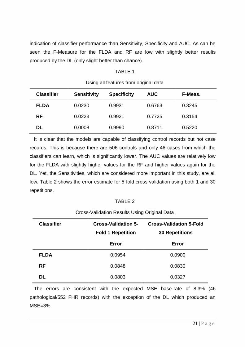
21 | P a g e
indication of classifier performance than Sensitivity, Specificity and AUC. As can be
seen the F-Measure for the FLDA and RF are low with slightly better results
produced by the DL (only slight better than chance).
TABLE 1
Using all features from original data
Classifier Sensitivity Specificity AUC F-Meas.
FLDA 0.0230 0.9931 0.6763 0.3245
RF 0.0223 0.9921 0.7725 0.3154
DL 0.0008 0.9990 0.8711 0.5220
It is clear that the models are capable of classifying control records but not case
records. This is because there are 506 controls and only 46 cases from which the
classifiers can learn, which is significantly lower. The AUC values are relatively low
for the FLDA with slightly higher values for the RF and higher values again for the
DL. Yet, the Sensitivities, which are considered more important in this study, are all
low. Table 2 shows the error estimate for 5-fold cross-validation using both 1 and 30
repetitions.
TABLE 2
Cross-Validation Results Using Original Data
Classifier Cross-Validation 5-
Fold 1 Repetition
Cross-Validation 5-Fold
30 Repetitions
Error Error
FLDA 0.0954 0.0900
RF 0.0848 0.0830
DL 0.0803 0.0327
The errors are consistent with the expected MSE base-rate of 8.3% (46
pathological/552 FHR records) with the exception of the DL which produced an
MSE=3%.

22 | P a g e
4.1.2 Model Selection
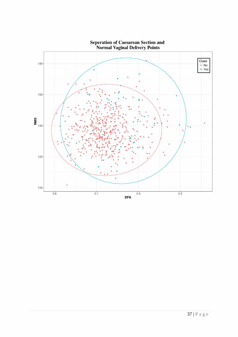
The receiver operator characteristic (ROC) curve is a useful graphic that shows the
cut-off values for the false and true positive rates. It is particularly useful in binary
classification to illustrate classifier performance. In the current evaluation, Figure 2
shows that the FLDA performed poorly. The RF and DL classifiers produced slightly
better results, which reflect the Sensitivity, Specificity and AUC values in Table 1.
The primary reason for the low Sensitivities (despite the AUC for the RF and DL
being relatively high) is that there are insufficient case records to model the class.
This is in contrast to the classification of control records that are skewed in its favour.
This causes significant problems in machine learning. As such, re-sampling the
classes in the absence of real pathological cases is a conventional way of
addressing this problem [59].
4.2 Using all Features from Synthetic Minority Over-Sampling Technique Data
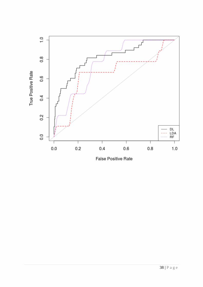
The 46 case records are re-sampled using the SMOTE algorithm. The SMOTE
algorithm generates a new dataset containing extra cases derived from the minority
class while reducing the majority class samples accordingly. Figure 3 shows the
separation of classes following oversampling. Compared with Figure 1 it is clear that
both case and control data are now evenly distributed between the two groups.
There is significant overlap between case and controls and no two feature
combinations were able to increase this decision boundary any further than that
presented in Figure 3.
4.2.1 Classifier Performance
Using the new SMOTEd feature set (300 cases and 300 controls – empirically this
distribution produced the best Sensitivity, Specificity, AUC, F-Measure and MSE
results), Table 3 indicates that the Sensitivities for all models improved (90% in most
cases). This is however at the expense of lower specificities (10% decreases). The
results are encouraging given that accurately predicting cases is more important
than predicting controls. The F-Measure acts as a support metric in this evaluation
and produces encouraging results in the RF and DL classifiers.
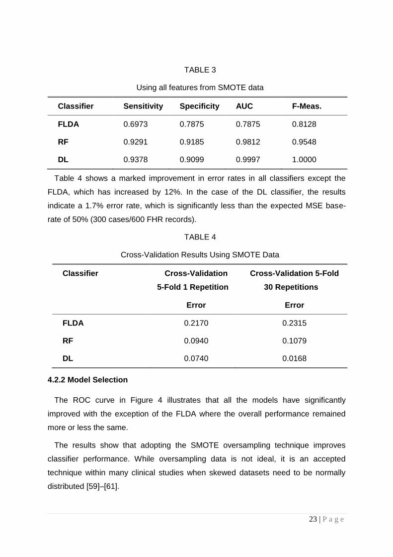
23 | P a g e
TABLE 3
Using all features from SMOTE data
Classifier Sensitivity Specificity AUC F-Meas.
FLDA 0.6973 0.7875 0.7875 0.8128
RF 0.9291 0.9185 0.9812 0.9548
DL 0.9378 0.9099 0.9997 1.0000
Table 4 shows a marked improvement in error rates in all classifiers except the
FLDA, which has increased by 12%. In the case of the DL classifier, the results
indicate a 1.7% error rate, which is significantly less than the expected MSE base-
rate of 50% (300 cases/600 FHR records).
TABLE 4
Cross-Validation Results Using SMOTE Data
Classifier Cross-Validation
5-Fold 1 Repetition
Cross-Validation 5-Fold
30 Repetitions
Error Error
FLDA 0.2170 0.2315
RF 0.0940 0.1079
DL 0.0740 0.0168
4.2.2 Model Selection
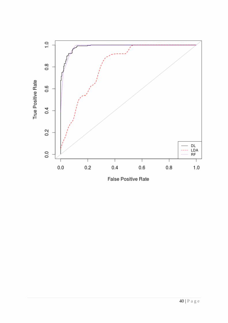
The ROC curve in Figure 4 illustrates that all the models have significantly
improved with the exception of the FLDA where the overall performance remained
more or less the same.
The results show that adopting the SMOTE oversampling technique improves
classifier performance. While oversampling data is not ideal, it is an accepted
technique within many clinical studies when skewed datasets need to be normally
distributed [59]–[61].
24 | P a g e
The remaining evaluations build on these results with a particular focus on
dimensionality reduction.
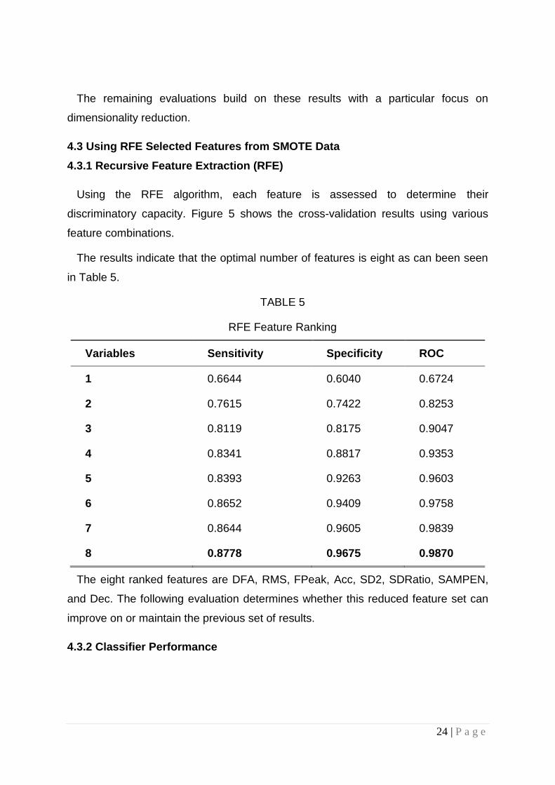
4.3 Using RFE Selected Features from SMOTE Data
4.3.1 Recursive Feature Extraction (RFE)
Using the RFE algorithm, each feature is assessed to determine their
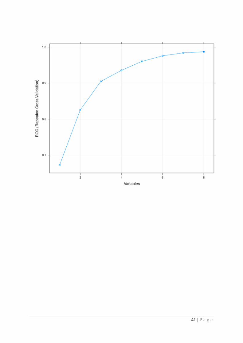
discriminatory capacity. Figure 5 shows the cross-validation results using various
feature combinations.
The results indicate that the optimal number of features is eight as can been seen
in Table 5.
TABLE 5
RFE Feature Ranking
Variables Sensitivity Specificity ROC
1 0.6644 0.6040 0.6724
2 0.7615 0.7422 0.8253
3 0.8119 0.8175 0.9047
4 0.8341 0.8817 0.9353
5 0.8393 0.9263 0.9603
6 0.8652 0.9409 0.9758
7 0.8644 0.9605 0.9839
8 0.8778 0.9675 0.9870
The eight ranked features are DFA, RMS, FPeak, Acc, SD2, SDRatio, SAMPEN,
and Dec. The following evaluation determines whether this reduced feature set can
improve on or maintain the previous set of results.
4.3.2 Classifier Performance
25 | P a g e
Looking at Table 6 it can be seen that most of the classifiers perform slightly worse
using the eight features in terms of Sensitivity. This is with exception to the RF
classifier, which can maintain similar results using the reduced feature set.
TABLE 6
Using RFE Features From Smote Data
Classifier Sensitivity Specificity AUC F-Meas.
FLDA 0.6169 0.7512 0.7564 0.7812
RF 0.9079 0.9135 0.9764 0.9138
DL 0.8314 0.8880 0.9980 1.0000
The MSE values, reported in Table 7, for all but the RF classifier (whose error
more or less stayed the same) were slightly worse than in the previous evaluation.
TABLE 7
Cross-Validation Results Using SMOTE Data with RFE
Classifier Cross-Validation
5-Fold 1 Repetition
Cross-Validation 5-Fold
30 Repetitions
Error Error
FLDA 0.2666 0.2719
RF 0.1068 0.1063
DL 0.0142 0.0343
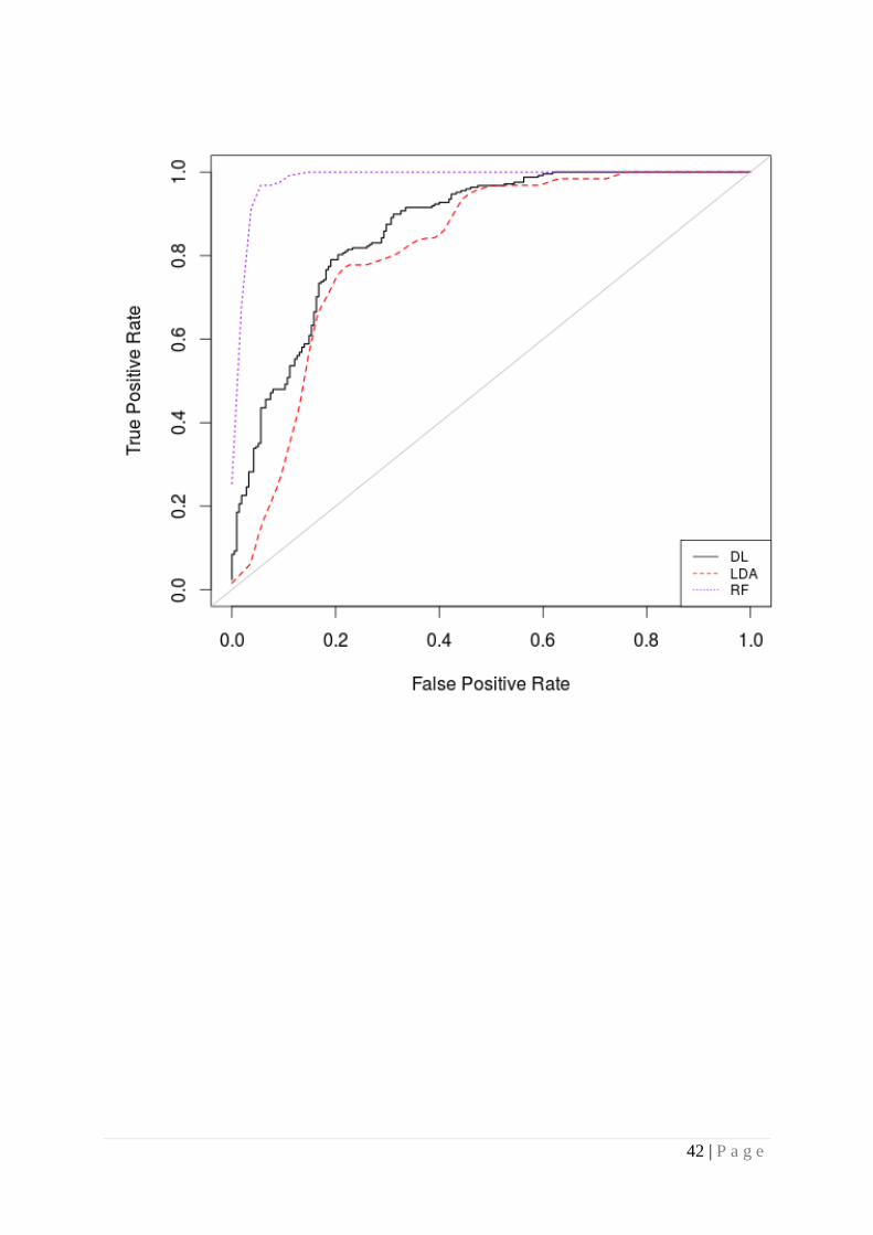
4.3.3 Model Selection
In this final evaluation, the ROC curve in Figure 6 illustrates that there are no real
improvements on the previous evaluation for the FLDA and DL, but that the RF
performs very well with a reduced set of features.
5 DISCUSSION
Obstetricians and midwives visually inspect CTG traces to monitor the wellbeing of
the foetus during antenatal care. However, inter- and intra-observer variability and
26 | P a g e
low positive prediction is accountable for the 3.6 million babies that die each year.
This paper, presented a proof-of-concept using machine learning and FHR signals
as an ambulatory decision support to antenatal care. The results indicate that it is
possible to provide high predictive capacity when separating normal vaginal
deliveries and caesarean section deliveries and in many cases produce much better
results than those reported in previous studies (see Table 8).
TABLE 8
Comparison of previous works
Paper Year Classifier Sensitivity Specificity
[22] 2013 Naïve Bayes 0.91 0.95
[6] 2014 RF and LCA 0.72 0.78
[62] 2013 LCR 0.66 0.89
[63] 2013 ANN 0.60 0.67
[25] 2012 SVM 0.73 0.76
[64] 2012 WFSS 0.92 0.88
[12] 2009 SI 0.90 0.75
[65] 2010 SVM 0.70 0.78
Using the original unbalanced dataset the best classifier (DL classifier) achieves
SE=0%, SP=99%, AUC=87%, and F-Measure=52%. While the Specificity values are
high, all Sensitivity values are below 3%. The low Sensitivity is attributed to the
disproportionate number of normal records compared with pathological records and
the fact that unbalanced datasets in general cause bias in favour of the majority
class. The minimum error rate MSE=3% was achieved by the DL using 30
repetitions. This relatively small MSE appeared to be a good error rate. However, the
classifiers were simply classifying by minimizing the probability of error, in the
absence of sufficient evidence to help them to classify otherwise.
The SMOTE algorithm using all 13 features significantly improved the Sensitivity
values for all classifiers. While oversampling is not ideal, it is a way to solve the class

27 | P a g e
skew problem that is widely used in medical data analysis [45], [66]–[71]. The best
classification algorithm is again the DL classifier, which achieves SE=94%, SP=91%,
AUC=100%, F-Measure=100% and MSE=2%. The reason for this is that the
algorithm has the ability to extract complex non-linear patterns generally observed in
physiological data like FHR signals. Through the extraction of these patterns, the DL
algorithm uses relatively simpler linear models for data analysis tasks, such as
classification. The DL generalizes, and finds the global minima, which allows it to
generate learning patterns and relationships beyond immediate neighbours in data. It
is able to provide much more complex representations of data by extracting
representations directly from unsupervised data without domain knowledge or
inference.
Using the RFE algorithm as a feature selection technique the algorithm eliminated
five features from the original 13 that were considered to have very low
discriminatory capacity. The remaining eight features were used to fit the models and
the results show that the RF achieved the best overall results with SE=91%,
SP=91%, AUC=98%, F-Measure=91% and MSE=11%.The primary reason for these
good results is that the RF algorithm is based on an ensemble of many randomized
decision-trees that are used to vote on the classification outcome. They are able to
handle data with a very large number of features (although the feature set in this
study is not particularly large) and those features that are important for classification
can be determined through the calculation of an importance score for each feature.
The score metric based on voting is similar to the approach adopted in k-nearest
neighbour classification and the voting mechanism to classify new data points based
on the majority surrounding data points of a particular class. The DL classifier
performed worse on the reduced dataset but still produces better results than several
studies discussed in this paper [6], [62], [25] and [65].
6 CONCLUSIONS AND FUTURE WORK
The primary aim in this paper was to evaluate a proof-of-concept approach to
separating caesarean section and normal vaginal deliveries using FHR signals and
machine learning. The results show that using a deep learning classifier it is possible
to achieve 94% for Sensitivity, 91% for Specificity, 99% for AUC, 100% for F-Score,

28 | P a g e
and 1% for Mean Square Error. This shows significant improvements over the 30%
positive predictive value achieved by obstetricians and midwives and warrants
further investigation as a potential decision support tool for use alongside the current
CTG gold standard.
Nonetheless, despite the encouraging results reported, the study needs further
evaluation using truly independent data to fully assess its value. In future work this
will be made possible by soliciting support for clinical trials and utilising other open
datasets that have adopted a similar study design. Other important work will include
regression analysis, using a larger number of classes to predict the expected
pathological event, in terms of the number of hours or days to delivery, not just
whether the outcome is likely to be a caesarean section or a normal vaginal delivery.
We also need to integrate and use the clinical data provided with this study in future
analysis tasks.
It will also be important to evaluate different parameter adjustment settings,
particularly in the case of the DL algorithm to determine if the results can be further
improved. Automatic feature detection will also be explored using the DL to extract
features from the raw FHR signals.
It is less than ideal to use oversampled data. Therefore, another direction for future
work will explore opportunities to obtain data through funded clinical trials. This will
also help provide a much more in-depth account of the value of machine learning
and its perceived benefits on predicting caesarean section and normal vaginal
deliveries.
While only the FHR signal is considered in this paper, since it provides direct
information about the foetus’s state, it would be useful to combine this signal with the
UC signal, which has been studied in previous work [72].
Overall, the proposed methodology is robust, contributes to the biomedical data
analytics field, and provides new insights into the use of deep learning algorithms
when analysing FHR traces that warrants further investigation.
7. ABREVIATIONS
CTG Cardiotocography
ST ST Segment connects the QRS Complex and the T wave

29 | P a g e
UHB University Hospital in Brno
CTU Czech Technical University
CTU-UHB Czech Technical University-University Hospital in Brno
STAN S21/S31 Product name for CTG Analysis
Avalon FM 40/50 Foetal monitor
FHR Foetal Heart Rate
UC Uterine Contraction
FIGO International Federation of Gynecology and Obstetrics
NICE National Institute for Health and Care Excellence
VBM Virtual Baseline
RBL Real Baseline
STV Short Term Variability
LTV Long Term Variability
RMS Root Mean Squares
SampEn Sample Entropy
FFT Fast Fourier Transform
PSD Power Spectral Density
FPeak Peak Frequency
HRV Heart Rate Variability
SD Standard Deviation
DFA Detrend Fluctuation Analysis
SVM Support Vector Machine
DL Deep Learning
RFE Recursive Feature Eliminator
SMOTE Synthetic Minority Oversampling Technique
SGD Stochastic Gradient Descent
FLDA Fishers Linear Discriminant Analysis
RF Random Forest
AUC Area Under the Curve
ROC Receiver Operator Curve
MSE Mean Square Errors
8. DECLERATIONS
8.1 Ethics approval and consent to participate
Not Applicable
8.2 Consent for publication
Not Applicable
8.3 Availability of data and material
The datasets generated during the current study are available in Physionet,
https://physionet.org/physiobank/database/ctu-uhb-ctgdb/
8.4 Competing interests
The authors declare that they have no completing interests

30 | P a g e
8.5 Funding
None Applicable
8.6 Authors' contributions
PF did all of the data processing and analysis, AH conducted the background
research, DA managed and conducted editorial reviews, DH and NB evaluated the
mathematical formulas and overall methodology. PF wrote the discussion and
conclusion sections.
8.7 Acknowledgements
None Applicable.
9. REFERENCES
[1] J. B. Warren, W. E. Lambert, R. Fu, J. M. Anderson, and A. B. Edelman, “Global neonatal and perinatal mortality: a review and case study for the Loreto Province of Peru,” Res. Reports Neonatol., vol. 2, pp. 103–113, 2012.
[2] R. Brown, J. H. B. Wijekoon, A. Fernando, E. D. Johnstone, and A. E. P. Heazell, “Continuous objective recording of fetal heart rate and fetal movements could reliably identify fetal compromise, which could reduce stillbirth rates by facilitating timely management,” Med. Hypotheses, vol. 83, no. 3, pp. 410–417, 2014.
[3] B. Chudacek, J. Spilka, M. Bursa, P. Janku, L. Hruban, M. Huptych, and L. Lhotska, “Open access intrapartum CTG database,” BMC Pregnancy Childbirth, vol. 14, no. 16, pp. 1–12, 2014.
[4] A. Ugwumadu, “Are we (mis)guided by current guidelines on intrapartum fetal heart rate monitoring? Case for a more physiological approach to interpretation,” Int. J. Obstet. Gynaecol., vol. 121, no. 9, pp. 1063–1070, 2014.
[5] A. Sola, S. G. Golombek, M. T. M. Bueno, L. Lemus-Varela, C. Auluaga, F. Dominquez, and E. Al., “Safe oxygen saturation targeting and monitoring in preterm infants: can we avoid hypoxia and hyperoxia?,” Acat Paediatr., vol. 103, no. 10, pp. 1009–1018, 2014.
[6] J. Spilka, G. Georgoulas, P. Karvelis, and V. Chudacek, “Discriminating Normal from ‘Abnormal’ Pregnancy Cases Using an Automated FHR Evaluation Method,” Artif. Intell. Methods Appl., vol. 8445, pp. 521–531, 2014.
[7] P. Pinto, J. Bernardes, C. Costa-Santos, C. Amorim-Costa, M. Silva, and D. Ayres-de-Campos, “Development and evaluation of an algorithm for computer analysis of maternal heart rate during labor,” Comput. Biol. Med., vol. 49, no. 1, pp. 30–35, 2014.

31 | P a g e
[8] J. Kessler, D. Moster, and S. Albrechfsen, “Delay in intervention increases neonatal morbidity in births monitored with cardiotocography and ST-waveform analysis,” Acta Obs. Gynecol Scand, vol. 93, no. 2, pp. 175–81, 2014.
[9] C. Rotariu, A. Pasarica, G. Andruseac, H. Costin, and D. Nemescu, “Automatic analysis of the fetal heart rate variability and uterine contractions,” in IEEE Electrical and Power Engineering, 2014, pp. 553–556.
[10] C. Rotariu, A. Pasarica, H. Costin, and D. Nemescu, “Spectral analysis of fetal heart rate variability associated with fetal acidosis and base deficit values,” in International Conference on Development and Application Systems, 2014, pp. 210–213.
[11] K. Maeda, “Modalities of fetal evaluation to detect fetal compromise prior to the development of significant neurological damage,” J. Obstet. adn Gynaecol. Res., vol. 40, no. 10, pp. 2089–2094, 2014.
[12] P. A. Warrick, E. F. Hamilton, D. Precup, and R. E. Kearney, “Classification of normal and hypoxic fetuses from systems modeling of intrapartum cardiotocography,” IEEE Trans. Biomed. Eng., vol. 57, no. 4, pp. 771–779, 2010.
[13] H. Ocak, “A Medical Decision Support System Based on Support Vector Machines and the Genetic Algorithm for the Evaluation of Fetal Well-Being,” J. Med. Syst., vol. 37, no. 2, p. 9913, 2013.
[14] T. Peterek, P. Gajdos, P. Dohnalek, and J. Krohova, “Human Fetus Health Classification on Cardiotocographic Data Using Random Forests,” in Intelligent Data Analysis and its Applications, 2014, pp. 189–198.
[15] A. Pinas and E. Chadraharan, “Continuous Cardiotocography During Labour: Analysis, Classification and Management.,” Best Pract. Res. Clin. Obstet. Gynaecol., vol. 30, pp. 33–47, 2016.
[16] P. A. Warrick, E. F. Hamilton, D. Precup, and R. E. Kearney, “Classification of Normal and Hypoxic Fetuses From Systems Modeling of Intrapartum Cardiotocography,” IEEE Trans. Biomed. Eng., vol. 57, no. 4, pp. 771–779, 2010.
[17] G. Koop, M. H. Pesaran, and S. M. Potter, “Impulse response analysis in nonlinear multivariate models,” J. Econom., vol. 74, no. 1, pp. 119–147, 1996.
[18] E. Blinx, K. G. Brurberg, E. Reierth, L. M. Reinar, and P. Oian, “ST waveform analysis versus cardiotocography alone for intrapartum fetal monitoring: a systematic review and meta-analysis of randomized trials,” Acta Obstet. Gynancelogica Scand., vol. 95, no. 1, pp. 16–27, 2016.
[19] H. Ocak, “A Medical Decision Support System Based on Support Vector Machines and the Genetic Algorithm for the Evaluation of Fetal Well-Being,” Springer J. Med. Syst., vol. 37, no. 9913, pp. 1–9, 2013.
[20] E. Yilmaz and C. Kilikcier, “Determination of Fetal State from Cardiotocogram Using LS-SVM with Particle Swarm Optimization and Binary Decision Tree,” Comput. Math. Methods Med., vol. 2013, no. 487179, pp. 1–8, 2013.

32 | P a g e
[21] H. Ocak and H. M. Ertunc, “Prediction of fetal state from the cardiotocogram recordings using adaptive neuro-fuzzy inference systems,” Neural Comput. Appl., vol. 23, no. 6, pp. 1583–1589, 2013.
[22] M. E. Menai, F. J. Mohder, and F. Al-mutairi, “Influence of Feature Selection on Naïve Bayes Classifier for Recognizing Patterns in Cardiotocograms,” J. Med. Bioeng., vol. 2, no. 1, pp. 66–70, 2013.
[23] E. M. Karabulut and T. Ibrikci, “Analysis of Cardiotocogram Data for Fetal Distress Determination by Decision Tree Based Adaptive Boosting Approach,” J. Comput. Commun., vol. 2, no. 9, pp. 32–37, 2014.
[24] D. Rindskopf and W. Rindskopf, “The value of latent class analysis in medical diagnosis,” Stat. Med., vol. 5, no. 1, pp. 21–27, 1986.
[25] J. Spilka, V. Chudacek, M. Koucky, L. Lhotska, M. Huptych, P. Janku, G. Georgoulas, and C. Stylios, “Using nonlinear features for fetal heart rate classification,” Biomed. Signal Process. Control, vol. 7, no. 4, pp. 350–357, 2012.
[26] E. Kreyszig, Advanced Engineering Mathematics. 2005.
[27] A. L. Goldberger, L. A. N. Amaral, L. Glass, J. M. Hausdorff, and E. Al., “PhysioBank, PhysioToolkit, and PhysioNet: Components of a new research resource for complex physiologic signals.”
[28] R. Mantel, H. P. van Geijn, F. J. Caron, J. M. Swartjies, van W. E. E., and H. W. Jongsma, “Computer analysis of antepartum fetal heart rate: 2. Detection of accelerations and decelerations,” Int. J. Biomed Comput, vol. 25, no. 4, pp. 273–286, 1990.
[29] J. Camm, “Heart rate variability: standards of measurement, physiological interpretation and clinical use. Task Force of the European Society of Cardiology and the North American Society of Pacing and Electrophysiology,” Circulation, vol. 93, no. 5, pp. 1043–65, 1996.
[30] S. Schiermeier, P. Van Leeuwen, S. Lange, Geue, D., M. Daumer, J. Reinhard, D. Gronemeyer, and W. Hatzmann, “Fetal heart rate variation in magnetocardiography and cardiotocography--a direct comparison of the two methods,” Z Geburtshilfe Neonatol., vol. 211, no. 5, pp. 179–84, 2007.
[31] M. G. Signorini, A. Fanelli, and G. Magenes, “Monitoring fetal heart rate during pregnancy: contributions from advanced signal processing and wearable technology,” Comput. Math. Methods Med., vol. 2014, no. 707581, pp. 1–10, 2014.
[32] D. Radomski, A. Grzanka, S. Graczyk, and A. Przelaskowski, “Assessment of Uterine Contractile Activity during a Pregnancy Based on a Nonlinear Analysis of the Uterine Electromyographic Signal,” in Information Technologies in Biomedicine, 2008, pp. 325–331.
[33] W. L. Maner, R. E. Garfield, H. Maul, G. Olson, and G. Saade, “Predicting term and preterm delivery with transabdominal uterine electromyography,” Obstet. Gynecol., vol. 101, no. 6, pp. 1254–1260, 2003.

33 | P a g e
[34] D. P. Williams, M. N. Jarczok, R. J. Ellis, and T. K. Hillecke, “Two-week test–retest reliability of the Polar® RS800CXTM to record heart rate variability,” Clin. Physiol. Funct. Imaging, vol. Online Fir, pp. 1–6, 2016.
[35] P. D. Welch, “The Use of Fast Fourier Transform for the Estimation of Power Spectra: A Method Based on Time Aver. aging Over Short, Modified Periodograms,” IEEE Trans. Audio Electoacoustics, vol. 15, no. 2, pp. 70–73, 1967.
[36] C. K. Karmakar, A. H. Khandoker, J. Gubbi, and M. Palaniswami, “Complex Correlation Measure: A Novel Descriptor for Poincare Plot,” Biomed. Eng. Online, vol. 8, no. 17, 2009.
[37] N. Sarkar and B. B. Chaudhuri, “An efficient differential box-counting approach to compute fractal dimension of image,” IEEE Trans. Syst. Man Cybern., vol. 24, no. 1, pp. 115–120, 1994.
[38] P. Abry, S. G. Roux, V. Chudacek, P. Borgnat, P. Goncalves, and M. Doret, “Hurst Exponent and IntraPartum Fetal Heart Rate: Impact of Decelerations,” in 26th IEEE International Symposium on Computer-Based Medical Systems, 2013, pp. 131–136.
[39] P. M. Granitto and A. B. Bohorquez, “Feature selection on wide multiclass problems using OVA-RFE,” Intel. Artif., vol. 44, no. 2009, pp. 27–34, 2009.
[40] R. Blagus and L. Lusa, “SMOTE for High-Dimensional Class-Imbalanced Data,” BMC Bioinformatics, vol. 14, no. 106, pp. 1–16, 2013.
[41] T. M. Khoshgoftaar, J. van Hulse, and A. Napolitano, “Comparing Boosting and Bagging Techniques with Noisy and Imbalanced Data,” IEEE Trans. Syst. Man Cybern. Syst., vol. 41, no. 3, pp. 552–568, 2011.
[42] N. V. Chawla, K. W. Bowyer, L. O. Hall, and W. P. Kegelmeyer, “SMOTE: Synthetic Minority Over-sampling Technique,” J. Artif. Intell. Res., vol. 16, pp. 321–357, 2002.
[43] T. Sun, R. Zhang, J. Wang, X. Li, and X. Guo, “Computer-Aided Diagnosis for Early-Stage Lung Cancer Based on Longitudinal and Balanced Data,” PLoS One, vol. 8, no. 5, p. 63559, 2013.
[44] L. M. Taft, R. S. Evans, C. R. Shyu, M. J. Eggar, and N. Chawla, “Countering imbalanced datasets to improve adverse drug event predictive models in labor and delivery,” J. Biomed. Inform., vol. 42, no. 2, pp. 356–364, 2009.
[45] W. Lin and J. J. Chen, “Class-imbalanced classifiers for high-dimensional data,” Brief. Bioinform., vol. 14, no. 1, pp. 13–26, 2013.
[46] J. Nahar, T. Imam, K. S. Tickle, A. B. M. S. Ali, and Y. P. Chen, “Computational Intelligence for Microarray Data and Biomedical Image Analysis for the Early Diagnosis of Breast Cancer,” Expert Syst. Appl., vol. 39, no. 16, pp. 12371–12377, 2012.
[47] Y. Wang, M. Simon, P. Bonde, B. U. Harris, and J. J. Teuteberg, “Prognosis of Right Ventricular Failure in Patients with Left Ventricular Assist Device Based on Decision Tree with SMOTE,” Trans. Inf. Technol. Biomed., vol. 16, no. 3, pp. 383–90, 2012.
34 | P a g e
[48] D. Silver, A. Huang, C. J. Maddison, A. Guez, L. Sifre, and E. Al., “Mastering the game of Go with Deep Neural Networks and Tree Search,” Nature, vol. 529, no. 7587, pp. 484–489, 2016.
[49] A. Candel, J. Lanford, E. LeDell, V. Parmar, and A. Arora, “Deep Learning with H20,” 2015.
[50] N. Srivastava, G. Hinton, A. Krizhevsky, I. Sutskever, and R. Salakhutdinov, “Dropout: A Simple Way to Prevent Neural Networks from Overfitting,” J. Mach. Learn. Res., vol. 15, no. Jun, pp. 1929–1958, 2014.
[51] I. Sutskever, O. Vinyals, and Q. V. Le, “Sequency to Sequency Learning with Neural Networks,” in 27th Annual Conference on Neural Information Processing Systems (NIPS), 2014, pp. 1–9.
[52] M. D. Zeiler, “ADADELTA: An Adaptive Laerning Rate Method,” arXiv.org, 2012. .
[53] P. Tomas, J. Krohova, P. Dohnalek, and P. Gajdos, “Classification of cardiotocography records by random forest,” in 36th IEEE International Conference on Telecommunications and Signal Processing, 2013, pp. 620–623.
[54] F. Tetschke, U. Schneider, E. Schleussner, O. W. Witte, and D. Hoyer, “Assessment of fetal maturation age by heart rate variability measures using random forest methodology,” Comput. Biol. Med., vol. 70, no. 1, pp. 157–162, 2016.
[55] R. Vressler, R. B. Kreisberg, B. Bernard, J. E. Niederhuber, J. G. Vockley, I. Shmulevich, and T. A. Knijnenburg, “CloudForest: A Scalable and Efficient Random Forest Implementation for Biological Data,” PLoS One, vol. 10, no. 12, p. e0144820, 2015.
[56] A. R. Webb and K. D. Copsey, Statistical Pattern Recognition. 2011.
[57] V. Lopez, A. Fernandez, S. Garcia, V. Palade, and F. Herrera, “An insight into classification with imbalanced data: Empirical results and current trends on using data intrinsic characteristics,” Inf. Sci. (Ny)., vol. 250, no. 20, pp. 113–141, 2013.
[58] J. Hand and R. J. Till, “A Simple Generalisation of the Area Under the ROC Curve for Multiple Class Classification Problems,” Mach. Learn., vol. 45, no. 2, pp. 171–186, 2001.
[59] L. Tong, Y. Change, and S. Lin, “Determining the optimal re-sampling strategy for a classification model with imbalanced data using design of experiments and response surface methodologies,” Expert Syst. Appl., vol. 38, no. 4, pp. 4222–4227, 2011.
[60] J. Spilka, G. Georgoulas, P. Karvelis, P. Vangelis, P. Oikonomou, V. Chudacek, C. Stylios, L. Lhotska, and P. Janku, “Automatic evaluation of FHR recordings from CTU-UHB CTG database,” Inf. Technol. Bio Med. Informatics, vol. 8060, pp. 47–61, 2013.
[61] R. Blagus and L. Lusa, “SMOTE for high-dimensional class-imbalanced data,” BMC Bioinformatics, vol. 14, no. 106, pp. 1–16, 2013.
35 | P a g e
[62] J. Spilka, “Complex approach to fetal heart rate analysis: A hierarchical classification mode,” 2013.
[63] A. Georgieva, S. J. Payne, M. Moulden, and C. W. G. Redman, “Artificial neural networks applied to fetal monitoring in labour,” Neural Comput. Appl., vol. 22, no. 1, pp. 85–93, 2013.
[64] R. Czabanski, J. Jezewski, A. Matonia, and M. Jezewski, “Computerized analysis of fetal heart rate signals as the predictor of neonatal acidemia,” Expert Syst. Appl., vol. 39, no. 15, pp. 11846–11860, 2012.
[65] V. Chudacek, J. Spilka, M. Huptych, G. Georgoulas, P. Janku, M. Koucky, C. Stylios, and L. Lhotska, “Comparison of Linear and Non-linear Features for Intrapartum Cardiotocography Evaluation–Clinical Usability vs. Contribution to Classification,” in Biosginal, 2010, pp. 369–372.
[66] L. M. Taft, R. S. Evans, C. r. Shyu, M. J. Egger, N. Chawla, J. A. Mitchell, S. N. Thornton, B. Bray, and M. Varner, “Countering imbalanced datasets to improve adverse drug event predictive models in labor and delivery,” J. Biomed. Informatics2, vol. 42, no. 2, pp. 356–364, 9AD.
[67] T. Sun, R. Zhang, J. Wang, X. Li, and X. Guo, “Computer-Aided Diagnosis for Early-Stage Lung Cancer Based on Longitudinal and Balanced Data,” PLoS One, vol. 8, no. 5, p. e63559, 2013.
[68] T. Sun, R. Zhang, J. Wang, X. Li, and X. Guo, “Computer-Aided Diagnosis for Early-Stage Lung Cancer Based on Longitudal and Balanced Data,” PLoS One, vol. 8, no. 5, p. e63559, 2013.
[69] J. Nahar, T. Imam, K. S. Tickle, A. B. M. Shawkat Ali, and Y. P. Chen, “Computational Intelligence for Microarray Data and Biomedical Image Analysis for the Early Diagnosis of Breast Cancer,” Expert Syst. Appl., vol. 39, no. 16, pp. 12371–12377, 2012.
[70] R. Blagus and L. Lusa, “SMOTE for High-Dimensional Class-Imbalanced Data,” BMC Bioinformatics, vol. 14, no. 106, 2013.
[71] Y. Wang, M. Simon, P. Bonde, B. U. Harris, J. J. Teuteberg, R. L. Kormos, and J. F. Antaki, “Prognosis of Right Ventricular Failure in Patients with Left Ventricular Assist Device Based on Decision Tree with SMOTE,” Trans. Inf. Technol. Biomed., vol. 16, no. 3, 2012.
[72] P. Fergus, P. Cheung, P. Hussain, D. Al-Jumeily, C. Dobbins, and S. Iram, “Prediction of Preterm Deliveries from EHG Signals Using Machine Learning,” PLoS One, vol. 8, no. 10, p. e77154, 2013.
Figure Legends
Fig. 1. Separation of Caesarean Section and Normal Vaginal Delivery Points
Fig. 2. ROC Curve for Original Data Using all Features

36 | P a g e
Fig. 3. Oversampled Separation of Caesarean Section and Normal Vaginal Delivery
Points
Fig. 4. ROC Curve for SMOTE Oversampled Data Using all Features
Fig. 5. RFE Feature Ranking
Fig. 6. ROC Curve for the Smote Data using RFE Features
37 | P a g e
38 | P a g e
39 | P a g e
40 | P a g e
41 | P a g e
42 | P a g e
Recommended