Pair Production in Real Proper Time and UnitarityWithout Borel Ambiguity
Cihan Pazarbası
Physics Department, Bogazici University 34342 Bebek / Istanbul, Turkey
Department of Physics, North Carolina State University, Raleigh, NC 27695, USA
Abstract
Pair production of scalar particles in general electromagnetic backgrounds is analyzed us-
ing real proper time effective action. Using the iε prescription, we show that contrary to
Euclidean time case, the real proper time construction preserves unitarity in an unambigu-
ous way. The ambiguity in the Euclidean case is analogous to the Borel ambiguity whose
treatment has been uncertain in problems with unstable vacua. Our construction clears
up this uncertainty by preventing existence of the Borel ambiguity in the first place. We
also discuss how this analysis is related to the WKB and path integral approaches to the
pair production problem and give a description of unambiguous pair production from a
geometric perspective using the latter one.
arX
iv:2
111.
0620
4v1
[he
p-th
] 1
1 N
ov 2
021
Contents
1 Introduction 1
2 Pair Production Problem and Resolution of Ambiguity 4
2.1 Ambiguity and its Resolution in Uniform Electromagnetic Background 5
3 Unambiguous Pair Production from Perturbative Expansions 9
3.1 Time Dependent Electric Fields: 12
3.2 Space Dependent Electric Fields: 13
4 Connection to Semi-Classics 14
5 Discussion and Prospects 19
1 Introduction
Particle pair production is one of the fundamental predictions of relativistic quantum the-
ories. Early on, it was noticed that this can be explained by modifications in the effective
Lagrangian of constant electromagnetic fields [1–3]. Later, in [4], using proper time for-
malism, Schwinger systematically showed that in the presence of constant electromagnetic
backgrounds, the effective Lagrangian (or action) develops an imaginary part which indi-
cates the vacuum instability so that particle creation. Since then, the particle production
in background electromagnetic fields has been investigated thoroughly for different types
of background potentials using different methods. (See [5, 6] for review on the subject.)
From a mathematical perspective, a consequence of the vacuum instability, so that the
particle creation, presents itself in the perturbation theory [7]: In QED, an expansion in the
fine structure constant α should be divergent, as the theory is ill-defined for negative values
of α. Although at first sight, a divergent series seems pathological, now it is understood in
the context of resurgence theory [8] that such series encodes all the physical information
in a consistent way.
A common way to decode this information is the Borel summation procedure. For
the pair production problem, this method was used in [9] for a solvable background elec-
tromagnetic field to obtain the pair production probability. The main goal of this paper
is obtaining the non-perturbative pair production probability from a Borel like procedure
while resolving another issue which is largely disregarded in the literature: Keeping the
theory unitary after the Borel process.
The unitarity problem shows itself in the ambiguous sign of the imaginary contribution
to the effective action. This is a general feature of the Borel procedure which stems from the
freedom of choice in the analytical continuation directions in the presence of singularities.
1

While these singularities are sources of non-trivial information, which can not be probed
by perturbative expansions, the freedom of choice leads to multi-valued physical quantities.
For problems with a stable vacuum, where the imaginary part should not exist in the
full solution, the problem has a resolution. Based on [10, 11], it has been precisely shown in
various settings [12–16] that the ambiguous imaginary contribution is canceled by inserting
additional non-perturbative information. In this way, the resulting quantity becomes real
and, maybe more importantly, unique. While this demonstrates a beautiful connection
between the perturbative and non-perturbative sectors of the theory, its not applicable to
systems with unstable vacua, as the imaginary part should not be canceled in these cases.
In the context of pair production, why the non-cancellation poses a problem can be
understood by investigating the vacuum-vacuum amplitudes. A vacuum instability presents
itself in vacuum-vacuum amplitude of the theory being less than one, i.e. S = 〈0|0〉 < 1.
In a time dependent setting, this amplitude is expressed as
S = 〈0+|U(∞,−∞)|0−〉, (1.1)
where |0±〉 are the vacua at infinite past and future while U is the unitary time propagator
connecting these two states. In general, the amplitude is a pure phase, i.e.,
S = eiΓ, (1.2)
where Γ is the effective action of the theory. As long as Γ ∈ R, the transition probability
|S|2 = 1 and the vacuum is a stable one, i.e. there is no creation of particles. However,
when Γ ∈ C, the transition probability becomes
|S|2 = e−2ImΓ ≤ 1. (1.3)
Obviously, whenever ImΓ 6= 0, the vacuum is not stable and there is a probability of particle
creation which is defined as
P = 1− |S|2 ∼ 2ImΓ. (1.4)
At this point, we make a critical observation. In (1.3), since the theory is unitary ImΓ
should not be negative. At first, this seems to be a trivial statement. However, to our
knowledge, this has been overlooked in pair production problems. For consistency and
completeness, the ImΓ > 0 condition should be implicit in methods we use.
In this paper, we are going to stress that consistent treatment can be achieved with
the Schwinger proper time integral but only when the proper time is chosen to be real.
This approach is motivated from two observations:
1. Schwinger’s proper time integral and the Borel integral have the same form.
2. When the proper time is chosen real, possible analytical continuation directions of
the integral are defined by construction.
The first point has been made previously (See e.g. for a recent discussion [17]). In
general, however, the divergent series for the perturbative effective action is found first,
2

then the Borel procedure is applied to tame the divergence and probe the singularity which
leads to the non-perturbative information, i.e the pair production probability in our case.
Instead of following this path, in this paper, we will probe these singularities before taking
the proper time integral. While the two approaches are equivalent, in this way, we will
keep the crucial analytical continuation information.
The predefined analytical continuation, on the other hand, stems from utilization of
the iε prescription. Its relation with the resolution of the Borel ambiguity was discussed
in [18–20]. Let us summarize the idea briefly: It is known that propagator(resolvent)
G±(u) = (u−H)−1 of a quantum theory is not well defined on the real u line [21]. Instead,
it is defined by an analytical continuation on the upper or lower half of the complex plane
by redefining G±(u) = limε→0(u± iε−H)−1. Then, any observable computed using these
redefined propagators have a certain predefined analytical continuation which prevents any
ambiguity in directions of the limit ε → 0. As we will see, these analytical continuations
determine the analytical continuation directions of the Schwinger’s integral contour when
the proper time is taken real instead of imaginary. Note that this redefinition also attributes
a time direction for the propagators and this will guide us to define the pair production
probability unambiguously.
We will discuss these two points in Section 2 and using the exact solution of Schwinger
to explain the resolution of the ambiguity problem for uniform electromagnetic back-
grounds. Then, in Section 3, we will extend our discussion to arbitrary backgrounds.
For this reason, we will use a recursive perturbative approach [22] which allows us to keep
track of the analytical continuation directions. While this method is analogous to the small
time expansion of heat kernels [23–25] and string inspired methods [26–28] in proper time
formalism of the quantum field theories, its recursive nature makes orders high enough to
probe non-perturbative effects computable.
Finally, in Section 4, we will connect the real time approach to two semi-classical ap-
proaches to the pair production problem. One approach is the WKB method, which treats
the pair production problem as a tunnelling problem [29–36]. Connection to the WKB
method helps us to understand what we really calculate in the perturbation discussion in
Section 3. The other approach is path integrals, which identify the pair production prob-
ability with the action of the classical equation of motion governed by the Hamiltonian of
the system. In pair production problems, the most common path integral approach is the
worldline instanton method [37–45]. It has been shown [46, 47] that the worldline instanton
method is equivalent to the semi-classical construction of Gutzwiller [48, 49], which has
also been linked to Lefschetz thimbles recently [50]. While our construction can be adapted
to any of these techniques, the discussion in Section 4 is closely related to the real time Lef-
schetz thimble description, which was shown to be an effective way to define semi-classical
path integrals in various contexts [51–54] including the pair production problem [55]. Here
this approach will help us to understand the Borel ambiguity resolution from a geometric
point of view.
3

2 Pair Production Problem and Resolution of Ambiguity
In this paper, we will only consider the pair production of bosonic matter as the fermionic
matter production can be handled equivalently and only constant prefactors would differ
in their results.
For bosonic matter fields in the presence of an electromagnetic background, the effec-
tive action at 1 loop order is expressed as
Γ(m2) =i
2ln det(m2 − H), (2.1)
where m2 is the mass of bosonic matter particles and
H =1
2(pµ − eAµ)2 (2.2)
is the Hamiltonian operator governing the motion of the bosonic particles. Note that in
this paper, we use gµν = diag(−+ ++) metric convention.
In a time-independent setting, the 1-loop effective action (2.1) can be expressed as
Γ±(m2) =
∫ m2
m20
dzTrG±(z), (2.3)
where G±(z) = (z ± iε− H)−1 is the Green’s operator, which should be defined via the iε
prescription and Γ±(m2) are defined as limits limε→0 Γ(m2 ± iε). G±(z) is not continuous
in ε→ 0 limit. We define a gap function which represents the discontinuity
∆Γ = Γ+(m2)− Γ−(m2) (2.4)
as our physical quantity and its imaginary part, Im∆Γ(m2), becomes the pair production
probability.
If we go to the time-dependent setting, the action in different branches is written as
Γ±(m2) = −i∫ ∞
0
dt
te±im
2t Tr e∓iHt, (2.5)
where we assumed the ε → 0 limit is already taken in respective branches. Note that it
is also possible to analytically continue t instead of m2. This is a much more convenient
approach in the time-dependent case and we will adapt it throughout the paper to extract
the imaginary contributions by rotating the contour in appropriate directions, i.e. upper
half-plane for Γ+ and lower half-plane for Γ−.
The gap ∆Γ(m2) originates from a branch cut of Γ(m2) on the complex m2 plane,
which is associated to simple poles of the integrand in (2.5) [56]. There is already a pole at
t = 0, which corresponds to the UV divergence in quantum fields theories and through the
renormalization procedure, they lead to the energy scale dependence of physical quantities.
In non-relativistic quantum mechanics [22], the author showed that t = 0 also acts as
a source for the semi-classical expansion which is intimately related to the perturbative
spectrum of the theory. On the other hand, the integrand has other possible singularities
at t 6= 0 which will be our focus in this paper.
4
Remark: The time evolution operator in (2.5) indicates that Γ± correspond to effective
actions for two different time evolutions, i.e, forward time evolution for Γ+ and backward
time evolution for Γ−. The latter can simply be seen by setting t → −t and re-writing it
as
Γ−(m2) = i
∫ 0
−∞
dt
teim
2t Tr e−iHt. (2.6)
Now, the action is described by forward time evolution between t = −∞ and t = 0.
Moreover, in this form the gap equation in (2.4) becomes
∆Γ(m2) = −i∫ ∞−∞
dt
teim
2t Tre−iHt (2.7)
which defines an action of transition between infinite past and future. Therefore, (2.7)
justifies the definition of the pair production probability as in (2.4) in an unambiguous way
Note that since the integration contour should be rotated in different directions for t > 0
and t < 0, throughout the paper we will use the integrals defined in (2.5) together with
the definition (2.4).
2.1 Ambiguity and its Resolution in Uniform Electromagnetic Background
Before considering general electromagnetic backgrounds, we are going to discuss how the
unambigous pair production rate emerges from the exact effective action in both uniform
electric and magnetic backgrounds and precisely show that the real proper time approach
leads to unambiguous results, which are consistent with the unitarity condition.
Before addressing the problem in real time, for completeness, let us first look at the
imaginary time case and show how the ambiguity arises. The 1 loop effective action in
Euclidean proper time for the bosonic fields in an electromagnetic background is 1
Γ(m) =1
8π2
∫ ∞0
ds
s3
e−sm2(seE)(seB)
sin(seE) sinh(seB). (2.8)
Note that similar to the real time case that we described above, one can always deform
the mass term as m2 → m2 ± ε and allow complexification of the proper time while
keeping the integral finite. However, this is not equivalent to the iε deformation in the
real time description and important information, which will allow us to keep unitarity,
is lost. The main reason behind this is that when we start with the Euclidean time,
the allowed/forbidden regions for forward and backward time evolutions are merged (See
Fig. 1). Therefore, the distinction between forward and backward time evolutions vanishes
and the expression (2.8) represents the effective action for both cases. This also prevents
from defining the gap ∆Γ unambiguously as in (2.4). This shows the origin of the ambiguity
in the Euclidean case and why its resolution needs a real time approach.
Let us review the standard picture for the pair production to emphasize its problem.
In (2.8), the poles related to the background electric field lie on the real axis at t = ±nπeE
while the poles corresponding to magnetic background are on the imaginary axis t = ±inπeB ,
1In the literature, sometimes the prefactor appears as 116π2 . The difference is due to 1
2factor in the
Hamiltonian (2.2).
5

t→ tE = te iπ2
t→ tE =te−iπ2
Real time: arg t ≥ 0
Real Time: arg t ≤ 0
Imaginary Time: arg t ≤ 0
Figure 1: Complex t planes. (Left) Real time cases: Regions allowed for analytical
continuations are represented by blue and disallowed regions are represented by red. (Right)
Imaginary time case: This is obtained by rotating real time ones by π2 in the respective
allowed directions. Note that blue and red regions on the right correspond to the same
regions on the right.
where n ∈ N+ for both cases. It is possible to compute the imaginary contributions using
standard contour integration. Common lore is that the electric poles lead to emergence
of ImΓ while the magnetic ones are not relevant since they do not lie on the integration
contour in (2.8).
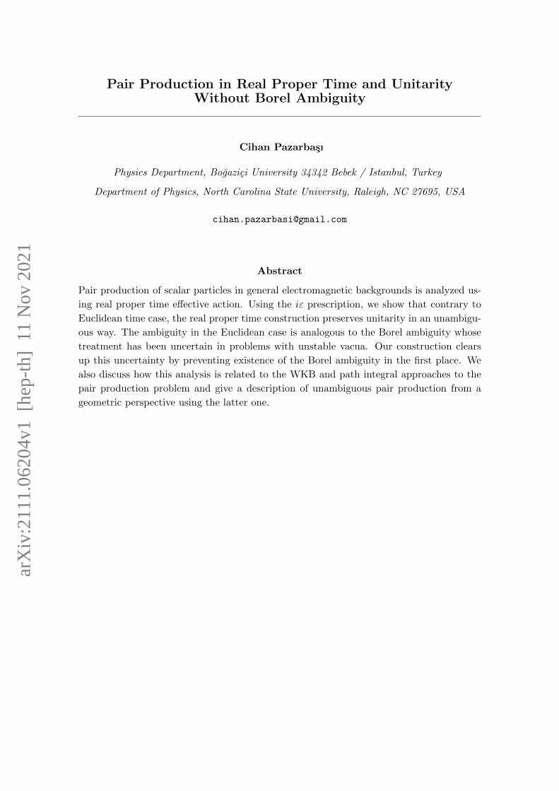
Consider the contribution of the first electric pole. There are two possible ways to
analytically continue which leads to two distinct integration paths, i.e. J+0 and J−0 . (See
Fig 2). There is no guideline for choosing any of these paths and this leads to complex
conjugate results:
ImΓ ∼ ∓e−m2πeE . (2.9)
We know that the pair production probability is defined by P ∼ 2ImΓ and can only be
positive. Therefore, we can just choose the result with + sign in (2.9). However, this
is an ad-hoc approach and does not hide the fact that the result is ambiguous. This is
equivalent to the Borel ambiguity and as we mentioned it can be overcome by real proper
time approach which provides us an ambiguous definition of the pair production probability
as we described above.
6

Re(t)
Im(t)
J+0
J−0
Figure 2: Possible paths to probe the singularity on the real axis. This picture describes
for the electric poles in the Euclidean case and the magnetic poles in the real time case.
Let us now return to the real proper time case. The effective action in real time is
Γ±(m) =1
8π2
∫ ∞0
dt
t3e±itm
2(teE)(teB)
sinh(teE) sin(teB). (2.10)
Note that the location of the poles related to electric and magnetic fields exchanged and
for both Γ± the possible analytical continuation directions are determined by definition.
In the following, for simplicity of discussion, we are going to continue with pure electric
field and pure magnetic field backgrounds.
Uniform Electric Background: In B → 0 limit, the effective action (2.10) becomes
Γ±(m) =1
8π2
∫ ∞0
dt
t3e±itm
2(teE)
sinh(teE)(2.11)
and the integrand has poles at
tE = ± inEπeE
, nE ∈ N+.
While all the poles can be treated collectively, the pair production rate of first particle and
anti-particle pair is only linked to the first order non-perturbative term [57, 58]. Therefore,
only this part needs to satisfy the unitarity condition without any ambiguity and we will
consider the first poles at tE = ± iπeE in our analysis.
For both Γ+ and Γ−, both poles at ± iπeE exist in the complex t plane. However, since
the analytical continuation of t is allowed only in one direction by construction, Γ+ and
Γ− can only get contributions from one of the poles, i.e., + iπeE or − iπ
eE respectively.
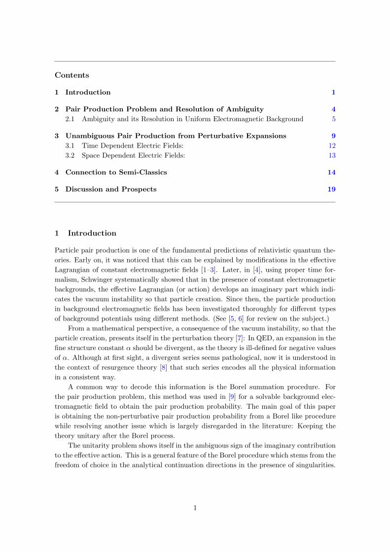
First, we consider Γ+(m). To get the contribution from the pole at iπeE , we simply
rotate the contour as in Fig. 3a and using∫J0
+∫−J−
π/2= 0, we re-write the effective action
as
Γ+(m2) = − eE8π2
∫J−π
2
dt
t2e−tm
2
sin(teE), (2.12)
where J−π/2 corresponds to the contour along the positive imaginary axis with a pre-defined
analytical continuation direction. Then, the contour integral in (2.12) leads to the imagi-
nary contribution
ImΓ+(m2) = +(eE)2
8π2e−
πm2
eE . (2.13)
7

J0
−J−π2
J∞
Re(t)
Im(t)
(a)
J0
−J+−π
2
J∞
(b)
Figure 3: Contours for the real time integrals in Electric case. 3a: Contours for Γ+. 3b:
Contours for Γ−.
In the same way, we can extract the imaginary part of Γ−(m2) from the pole at − iπeE . This
time, we rotate the contour as in Fig. 3b and re-write the effective action as
Γ−(m2) = − eE8π2
∫J+−π2
dt
t2e−tm
2
sin(teE). (2.14)
This is the same integral with only difference is that the direction of the contour J+−π
2is
now along the negative real axis. Then, we get the imaginary part of Γ− as
ImΓ−(m2) = −(eE)2
8π2e−
πm2
eE . (2.15)
Combining these two results, we get the imaginary part of the gap ∆Γ(m2) = Γ+(m2) −Γ−(m2), so that the pair production rate as
P = Im∆Γ(m2) =(eE)2
4π2e−
πm2
eE , (2.16)
which recovers the standard pair production probability P ∼ e−2ImW with an unambigous
sign. Note that along with the individual results for ImΓ±, the unambigous definition of
∆Γ is also a primary factor for the unambiguous end result. Without this definition, the
ambiguity would be persistent in the real time case in the same way with the Euclidean
case.
Remark: The rotations of the initial contours in both cases are equivalent to respective
proper Wick rotations and the resulting integrals are the same with the ones written in
the imaginary proper time (2.8). However, since we started with the real time, contrary
to the imaginary proper time case, the analytical continuation directions around the poles
are pre-determined, so there can not be any ambiguity in the signs of the imaginary parts
of Γ±(m2) arising from them. Moreover, with these proper Wick rotations, we can match
the Euclidean time contours in Fig. 2 with the real time contours in Fig 3 as J−0 ←→ J−π2
and J+0 ←→ J+
−π2.
8

Uniform Magnetic Background: Although the uniform magnetic case does not yield
pair production, for completeness, we will also show how it fits in our treatment. In E → 0
limit, (2.10) reduces to
Γ±(m2) =1
8π2
∫ ∞0
dt
t3e±itm
2(teB)
sin(teB). (2.17)
Now the poles are on the real axis and the treatment is similar to the standard Borel
integral. However, again as in the electric background case, the restriction on the an-
alytical continuation directions for both Γ+ and Γ− prevents ambiguous results. Tak-
ing the integrals using the appropriate contours as pictured in Fig. 2, we find the gap
∆Γ(m) = Γ+(m)− Γ−(m) due to the pole at tB = πeB as
∆Γ =eB
8π2
[(−iπ)
(eB)
π2eiπm2
eB − (+iπ)eB
π2e−
iπm2
eB
]=
(eB)2
4π3sin
(πm2
EB
)(2.18)
which is manifestly real as expected.
Note that the emergence of a pure real result in (2.18) is analogous to the well-known
cancellation between the imaginary contribution of the Borel summation process and the
non-perturbative contributions to a stable vacuum. As we will show in the next section, the
poles on any part of the complex t plane are analogous to the Borel singularities arising from
the summation of a perturbative expansion. However, contrary to the standard approach in
the real time approach we described above, there is no need for additional non-perturbative
contributions for the cancellation. This is similar to the Lefschetz thimble approach, where
the cancellation of the imaginary parts originates from the different saddles. In Section 4, in
a specific example, we will discuss the pair production problem form a similar point of view
and show that the nature of contributing saddles is intimately related to arg t. This effects
the paths contributing to the integral on complex space and, as we will show, these paths’
behaviours are consistent with the cancellation in the magnetic case and non-cancellation
in the electric case.
3 Unambiguous Pair Production from Perturbative Expansions
In physics, exact solutions are very rare. Therefore, while the discussion in Section 2.1
explicitly show how the pair production rate in the presence of a uniform electric field
emerges in a way that the unitarity is preserved, it is also important to show how the same
information can be achieved when an exact solution is not possible.
In absence of an exact solution, perturbative techniques allow us to compute the co-
efficients in a perturbation expansion, which form generically divergent series. The non-
perturbative information is encoded in this divergent series and can be extracted using
Borel-Pade techniques [59–61]. However, the Borel-Pade summation leads to the same
ambiguity that we discussed in the Euclidean case in the previous section and whenever
there is a persistent instability of the vacuum. As in the uniform case, the resolution comes
from the real time approach. To get an unambiguous result, the poles of the propagator
9

should be probed directly, i.e. we need to sum the perturbative expansion of the propaga-
tor U(t) = Tre±itH in (2.5) before taking the proper time integral. For this reason, we are
going to adapt the recursive perturbative scheme introduced in [22] which is based on the
construction in [62, 63]. In [22], it was shown that the non-commutativity of phase-space
variables acts as a source for a derivative expansion which is identified as the semi-classical
expansion. In the present context, the non-commutativity again produces a derivative ex-
pansion which corresponds to the deviation from the uniform field2. At each order of the
derivative expansion, there is also another expansion which depends on the electromagnetic
field strength and using this one the non-perturbative pair production probability at each
order in the derivative expansion can be obtained. Note that this approach has already
been applied to an exactly solvable case in [9]. In this section, we will show how those
results can be obtained for arbitrary background fields using a finite order perturbative
expansion.
In this section, we will investigate pure electric fields. The Hamiltonian is written in
general as
H = −1
2(p0 − eA0(x))2 +
1
2(p− eA(x0))2 ≡ −1
2π2
0(p0,x) +1
2π2(p, x0). (3.1)
We assume that the gauge potential has the following form
Aµ(x0,x) = −Eω
(H0(ω x),H(ω x0)) (3.2)
so that the electric field is E = E(
dH(x0)dx0
+∇H0(ω x))
. Since we are mainly interested
in the locally uniform fields, we assume that both H0(ωx) and H(ωx0) are slowly varying
functions of x and x0 respectively. For the same reason, we also assume that m2 � eE � ω
throughout this section. This will guide us in our calculations.
The effective action for the Hamiltonian in (3.1) is written as
Γ±(m2) = −i∫ ∞
0
dt
te±im
2t
∫dp0 dp
(2π)4〈p0,p|e∓it(−
12π20(p0,x)+ 1
2π2(p,x0))|p, p0〉. (3.3)
Note that since π0 and π do not commute with each other, the propagator does not
factorize trivially. To get the perturbative expansion, we can either redefine the propagator
U(t) = Tre∓itH as
U(t) = e±itπ202 U(t) (3.4)
or
U(t) = e∓itπ2
2 U(t). (3.5)
As shown in [22], both choices are equivalent. Solving the time dependent Schrodinger
equation for redefined propagators and following the steps in [22], we reach a recursive
2Although, the derivative expansion we will consider in this paper is not the semi-classical expansion as
in [22], these two expansion are related to each other with a redefinition of expansion parameters. See e.g.
[64].
10

expansion for U(t) for each case and express the effective action in terms of this recursive
expansion.
Let us consider pure time dependent and pure space dependent electric fields. For the
time dependent case, where A0(x) = 0 and π0 = p0, the perturbative expansion is written
as
Γ±time(u) = −i∑m=0
∫ ∞0
dt
te±im
2t
∫dp0 dx0 d3p
(2π)4e∓
iπ2t2
m∑k=1
U±m,k(t) e∓ ip
20t
2 , (3.6)
where U± is given by the recursion relation
U±m,k(t) =m−k+1∑l=1
~l
l!
∂lπ2
∂xl0
∫ t
0dt1 bl±(p0, ∂p0 , t1)U±m−l,k−1(t1), (3.7)
with the initial value U±0,0 = 1 and the operator valued function
b±(p0, ∂p0 , ti) = i∂p0 ± p0 ti ∓ p0 t. (3.8)
Note that equations (3.6) - (3.8) indicate that the problem is effectively a one dimensional
one regardless the details of the background gauge field.
If the background field, on the other hand, is space dependent, then the problem might
be a multi-dimensional one. In this case, A(x0) = 0 , π = p and the perturbative expansion
becomes
Γ±space(u) = −i∑m=0
∫ ∞0
dt
te±im
2t
∫dp0 d3p dDx
(2π)4e∓
iπ0t2
m∑k=1
U±m,k(t) e∓ ip
2t2 , (3.9)
where U± is
U±m,k(t) =m−k+1∑l=1
~l
l!∇lπ2
0
∫ t
0dt1 bl±(p,∇p, t1) U±m−l,k−1(t1), (3.10)
with U±0,0 = 1 and
b±(p,∇p, ti) = i∇p ± p ti ∓ p t. (3.11)
Note that the dimension D of the space integral depends on the dimensionality of A0(x).
Even though it does not change the general structure of pair production probability, it
plays a role in prefactors. We will elaborate this, when we discuss the space dependent
fields.
Remark: Equations (3.7) and (3.10) shows that the expansion is a semi-classical one.
However, in this section, we set ~ = 1, since the only expansion parameters we are interested
in are ω and eE . When the pair production problem is considered as a semi-classical
approximation after redefining parameters ~, ω, eE , the pair production probability is given
by the classical action, i.e. m = 0 term in (3.6) and (3.9) [64]. We will use this information
Section 4, when we compare our method to the semi-classical approaches.
11

Using the recursive formula, we can now compute the perturbative expansion of the
integrand Tre∓iHt
t in powers of ω and g = eE . This is a double expansion which is formally
expressed asTre∓itH
t=∑m,n
αm,n(t)ω2mg2n. (3.12)
The poles of the integrand at t 6= 0 are related to the summation of this double series. This
poses a problem of summation order. The order of summation should be chosen according
to the dominance of the expansion variables ω and g. Since m � g � ω while summing
the series in (3.12), we keep the order of ω constant and sum over the g expansion.
In the following, we will analyze general time dependent and space dependent cases in
4 dimensional space-time dimensions and compute the leading order non-perturbative pair
production probability, which is obtained from the series at O(ω0), while postponing the
analysis of corrections to this leading order for the future.
3.1 Time Dependent Electric Fields:
We first consider time dependent electric fields for
A(x0) =Eω
H(ωx0). (3.13)
As we stated above, this is effectively a one-dimensional problem. Although this has already
been treated by the exact WKB method [36], here using the recursion relation and the
Pade summation of perturbative expansion of the propagator, we will obtain unambiguous
version of the pair production probability.
Using the recursion formula (3.7), we compute the expansion at order O(w0) up to x0
integral:∑n=0
α0,n g2n =
1
4π2it3
[1− (gtH′)2
24+
7(gtH′)4
5760− 31 (gtH′)6
967680+
127 (gtH′)8
154828800− 73 (gtH′)10
3503554560+ . . .
](3.14)
where H′ = dH(ωx0)dx0
. In (3.6), before integrating over p, we rescaled the momentum as
p→ p + A(x0) and in this way, all momentum integrals become Gaussian. Note that due
to the sign change in Lorentzian metric, prefactor of the Gaussian integrals comes up as1
(√
2πit)3√−2πit
= 14π2it2
rather than standard prefactor of 4 dimensional Gaussian integrals(1√
2πit2
)4= − 1
4π2t2. Overall imaginary factor is important as it contributes to the effective
action directly.
The series in (3.14) is a convergent one. It becomes divergent if we take the proper
time integral directly, which can be treated by the Borel-Pade procedure. In this sense, the
expansion we computed in (3.14) can be considered as a Borel summed series. Therefore,
we can directly probe the singularity structure represented by this series using the Pade
summation.
First two terms in the expansion are singular at t = 0. They correspond to the UV
divergent terms and can be treated by renormalization. It is possible to ignore them in
12

Pade approximation when probing the poles at finite t, however, we observe that they play
a role in the constant part of the prefactor of the effective action. Although it does not
have a physical implication, we prefer to keep them in the calculations for completeness.
Then, we write the effective action at order O(ω0) as
Γ±ω0 = −
∫R
dx0
∫ ∞0
dt e±im2t
4π2t3
∑n=0
α0,n
(gtH′
)2n. (3.15)
Pade summation of term up to O(g26) leads non-zero singularities at
gH′t? = ±π {1.0000i, 2.0000i, 2.9994i} . (3.16)
As we indicated in the previous section, only the first pole is linked to the pair production
probability. Therefore, we express the effective action as
Γ±ω0 ' −
∫R
dx0
∫ ∞0
dt e±im2t
4π2t31
(iπ)2 − (gH′t)2 . (3.17)
As in the uniform case, we compute the imaginary parts by rotating the initial contour for
t integral in appropriate directions as in Fig. 3. Then, we find the imaginary part as
ImΓ±ω0(m2) = ±
∫R
dx0(gH′(ωx0))2
8π3e− m2πgH′(ωx0) . (3.18)
This form of the effective action at the leading order of the derivative expansion is already
known as local field approximation [65, 66] and can be evaluated for specific cases for H′
(See e.g. [9]). Instead, we handle the integral by saddle point approximation, which is
possible since m� g and H(ωx0) is chosen to be slowly varying. For this reason, we make
the following general assumptions for H around the saddle point:
i) H′(ωx?0) = h0 , ii) H′′(ωx?0) = 0 , iii) H′′′(ωx?0) = −h2ω2 , h2 6= 0, (3.19)
where second assumption simply follows from the saddle point approximation while first one
states that electric field E is constant, i.e. independent of ω, at the saddle point x?0 so the
field is locally uniform as we assumed at the beginning. Finally, third assumption indicates
deviation from the uniform case while assuring the saddle point x?0 is non-degenerate and
h2 is a constant differs for different backgrounds. With these assumptions, we get the
leading order pair production probability as
∆Γω0(m2) '√
2 (|h0|g)5/2
4π3m |h2|1/2 ωe− m2π|h0|g , (3.20)
where h0 and h2 can be determined for specific background fields.
3.2 Space Dependent Electric Fields:
Now, we will consider space-dependent pure electric backgrounds for
A0(x) =EωH0(ωx). (3.21)
13
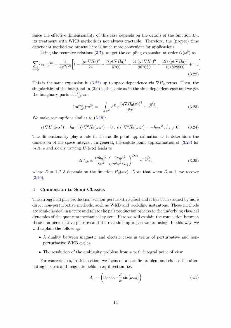
Since the effective dimensionality of this case depends on the details of the function H0,
its treatment with WKB methods is not always tractable. Therefore, the (proper) time
dependent method we present here is much more convenient for applications.
Using the recursive relations (3.7), we get the coupling expansion at order O(ω0) as∑n=0
α0,n g2n =
1
4π2it3
[1− (gt∇H0)2
24+
7(gt∇H0)4
5760− 31 (gt∇H0)6
967680+
127 (gt∇H0)8
154828800+ . . .
](3.22)
This is the same expansion in (3.22) up to space dependence via ∇H0 terms. Then, the
singularities of the integrand in (3.9) is the same as in the time dependent case and we get
the imaginary parts of Γ±ω0 as
ImΓ±ω0(m2) = ±
∫RD
dDx(g∇H0(x))2
8π3e− m2πg∇H0 . (3.23)
We make assumptions similar to (3.19):
i)∇H0(ωx?) = h0 , ii)∇2H0(ωx?) = 0 , iii)∇3H0(ωx?) = −h2w2 , h2 6= 0. (3.24)
The dimensionality play a role in the saddle point approximation as it determines the
dimension of the space integral. In general, the saddle point approximation of (3.23) for
m� g and slowly varying H0(ωx) leads to
∆Γω0 '(gh0)2
8π3
(2πgh2
0
m2ω2πh2
)D/2e−m
2πgh0 , (3.25)
where D = 1, 2, 3 depends on the function H0(ωx). Note that when D = 1, we recover
(3.20).
4 Connection to Semi-Classics
The strong field pair production is a non-perturbative effect and it has been studied by more
direct non-perturbative methods, such as WKB and worldline instantons. These methods
are semi-classical in nature and relate the pair production process to the underlying classical
dynamics of the quantum mechanical system. Here we will explain the connection between
these non-perturbative pictures and the real time approach we are using. In this way, we
will explain the following:
• A duality between magnetic and electric cases in terms of perturbative and non-
perturbative WKB cycles.
• The resolution of the ambiguity problem from a path integral point of view.
For concreteness, in this section, we focus on a specific problem and choose the alter-
nating electric and magnetic fields in x3 direction, i.e.
Aµ =
(0, 0, 0,−E
ωsin(ωx0)
)(4.1)
14

for the electric case and
Aµ =
(0, 0,−E
ωsin(ωx1), 0
)(4.2)
for the magnetic case. In addition we keep p0 for the electric case and p1 for the magnetic
case and set the other components of momenta to zero as they only play a role in the
prefactor. Then, the corresponding Hamiltonians are written as
HE = −p20
2+
g2E
2ω2sin2(ωx0) , gE = eE (4.3)
HB =p2
1
2+
g2B
2ω2sin2(ωx1) , gB = eB. (4.4)
The semi-classical aspects of this system are well studied in both worldline formalism
[38, 39] and WKB formalism [30, 64]. In fact, in these settings, the exponent of the pair
production probability is just the classical action of the system, i.e. S0 ∼ m2πeE . In the
following, for simplicity, we will drop the variables g and ω as they don’t play a role in the
qualitative discussion we will pursue.
Recall from (3.6),(3.9) and (3.7), (3.10) that the classical actions for electric and mag-
netic backgrounds are respectively
Γ±E = −i∫ ∞
0
dt
te±im
2t
∫dx0dp0
2πe∓it sin2(x0)e±
ip20t
2
= −i∫ ∞
0
dt
t√∓2πit
e±im2t
∫R
dx0 e∓it sin2(x0) (4.5)
and
Γ±B = −i∫ ∞
0
dt
te±im
2t
∫dx1dp1
2πe∓it sin2(x1)e∓
ip21t
2
= −i∫ ∞
0
dt
t√±2πit
e±im2t
∫R
dx1 e∓it sin2(x1). (4.6)
These integrals will be the basis of the following discussion on WKB and path integral
approaches.
Duality of WKB Cycles: In order to see the equivalence to the standard WKB inte-
grals, we first take the t integral after rotating its contour by ±π2 . Then, we find
∆ΓB(m2) =√
2
∮dx1
√m2 − sin2(x1) (4.7)
and
∆ΓE(m2) = i√
2
∮dx0
√m2 − sin2(x0) (4.8)
In these expressions, the main difference between the electric and magnetic cases is the
imaginary prefactor. In fact, (4.7) and (4.8) can be thought as action and dual action of
15

the same theory [67–69]. To see this clearly, let us take the imaginary factor in (4.8) into
the square root term and express it as
∆ΓE(m2) =√
2
∮dx0
√−m2 + sin2(x0)
=√
2
∮dx0
√m2 − cos2(x0) (4.9)
where m2 = 1 − m2. Because of the phase difference between sin2(x) and cos2(x), the
perturbative and non-perturbative WKB cycles in electric and magnetic cases exchange.
This shows the duality between the two actions in (4.7) and (4.8) or between the magnetic
and electric cases.
Another way to understand this duality is making the observation that the electric
potential corresponds to the inverted magnetic potential with an unimportant scaling. The
connection between inverting the potential and the duality was investigated in [70] using
the connection between one dimensional quantum mechanics and holomorphic anomaly
equations, where the authors shows that the analysis for the dual case is done around the
top of the inverted potential. In our setting, the source of this inversion- and therefore
the duality- is the Minkowskian metric. Moreover, this observation shows that we make
our perturbative analysis around the dual (non-perturbative) vacuum which corresponds
to the top of the inverted potential3. We will use this information in our analysis of the
path integral perspective.
Cancellation and Non-cancellation from Path Integrals: Now, turning back to
the integrals in (4.5) and (4.6), we will show the cancellation or non-cancellation of the
imaginary contributions from path integral perspective. Note that in (4.5) and (4.6), the
space integrals are one dimensional not infinite dimensional. This is not introduced for any
simplification; instead, they correspond to the exact classical limit of the theory.
The space integral is the same for both magnetic and electric cases :
I± =
∫R
dx e∓it sin2(x), (4.10)
where we set g = ω = 1 as they don’t play a role in the following discussion. Note that this
integral form was investigated in [14] in a finite region and the cancellation of the Borel
ambiguity was explained. Their analysis corresponds to the imaginary proper time version
of our discussion. We will follow similar arguments for (4.10) but also use the lessons of
previous sections which will lead us to the resolution of the ambiguity. Then, at the end
of the section, we will compare these two analyses.
The critical point is on the initial contour, the integral in (4.10) is not convergent due
to the oscillating behaviour of its exponent. To prevent this problem, we should express
3This is known for the uniform case as the uniform electric field background corresponds to the inverted
harmonic oscillator. However, our description indicates that this is also valid for more general background
potentials. Although, we used simple cos2(x) = 1− sin2(x) relationship in (4.9) and re-scaled m2 → 1−m2
, these transformations have a geometric origin related to the duality between the two action. (See [71] for
details.)
16

this path integral in terms of paths which behaves as e−t sin2(x) as |x| → ∞. Among all
possible such paths, we will choose the steepest descent ones since they have the most
dominant contributions. In the following, we will label these paths with J and we will
label the other paths, which don’t converge exponentially as |x| → ∞, with K. These are
called the Lefschetz thimbles and they are closely related to the Morse theory. We will
not discuss their construction since we are only interested in their roles in cancellation
mechanism in the pair production problems. For details on the subject see [72, 73].
Due to the periodic nature of the potential, we can focus only on the region [−π2 ,
π2 ]
and investigate contribution of the paths passing through the extremum point x = 0, which
represents stable/unstable vacuum of theory, to the integral (4.10) for different values of
arg t. Remember that for electric and magnetic cases, the singularities on the complex
proper time plane appear in different regions and we needed to deform the proper time
integral accordingly. We will use this information here as our guide to investigate the
behaviour of the spatial integral on complex x plane and in this way, we will describe the
resolution of the ambiguity in path integral perspective.
Magnetic Case: Let us start with the magnetic field background. We know that in
this case, the non-perturbative information arises from arg t = 0± for Γ±(m2) . Since the
integrands have oscillating behaviours in both cases, the real part of the exponent should
be constant along the integration path:
Re sin2(x) = const (4.11)
The imaginary parts should behave differently along these paths due to the sign difference
in the exponent. Therefore, as |x| → ∞, the conditions
Im[t sin2(x)
]< 0 (4.12)
for arg t = 0+
Im[t sin2(x)
]> 0 (4.13)
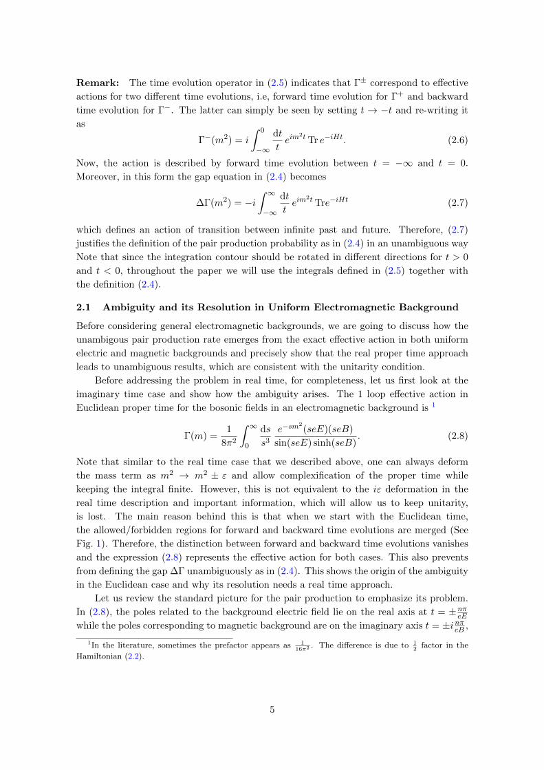
for arg t = 0− should be satisfied. Corresponding regions and associated contours J ±B and
K±B are shown in Fig. 4a. Despite the allowed paths are different for two cases, their
tails directing to imaginary infinities cancel each other. Therefore, both of the are well
defined and the remaining parts are just the original integral (4.10). Moreover, the gap
∆ΓB = Γ+B − Γ−B corresponds to the perturbative WKB cycle. All of these are consistent
with the expected oscillatory behaviour.
Electric Case: Now, we turn to the electric field background and focus on the behaviour
of the integrals around arg t = ±π2∓. Around these regions, the spatial integral becomes
I± =
∫R
dx et sin2(x), (4.14)
which can be interpreted as inverted potential case. The integrand in (4.14) is real. Then,
in this case, the imaginary part should be constant along the integration contour:
Im sin2(x) = const. (4.15)
17

J +B
K+B
J−BK−B
(a)
K+E
J +E
K−E
J−E
(b)
Figure 4: Spatial contours for the magnetic case (left) for arg t = ±0.1 and the electric
case (right) for arg t = ±π2 ∓ 0.1. In Lighter regions the integrals converge while they
diverge in darker regions. Paths for convergent integrals, i.e. J ±B and J ±E , are plotted in
red while paths for the divergent ones, i.e. K±B and K±E , are plotted in blue.
In both cases, as |x| → ∞, the integration paths should pass through regions corresponding
to
Re[t sin2(x)
]< 0. (4.16)
The integration paths J ±E and K±E are shown in Fig 4b. Contrary to the magnetic case,
this time the allowed regions are the same and the Lefschetz thimbles pass through the
same regions in opposite directions. Therefore, their contribution to ∆Γ = Γ+ − Γ− is a
constructive one rather than a destructive one as we observed in Sections 2.1 and 3. This
explains the ambiguity resolution from a geometric perspective.
18

Comparison: These two examples are illustrations of how real time approach resolves
the Borel ambiguity from path integral point of view. Note that the electric case is very
similar to [14], where ∫dt e−tE sin2(x) (4.17)
was considered. Main difference between two analysis is that the roles of regions in complex
space exchanged. This is because the electric case corresponds to the inverted potential
version, i.e. V ∼ − sin2(x), as we discussed in WKB approach. In [14], paths represented
by K±E in Fig. 4b are the Lefschetz thimbles corresponding to analytical continuations from
arg tE and the integral is convergent along these paths. Note that their behaviour around
infinities are very different. This is due to a jump at arg tE = 0, which is called the Stokes
phenomenon and it is the source of the Borel ambiguity.
In our case, on the other hand, both J +E and J −E approach to imaginary axis as
arg t → ±π2∓, which corresponds to arg tE = 0 for the Euclidean case as we discussed
in Section 2.1. They flow towards opposite directions. This is analogous to the Stokes
phenomenon but due to the prescription we used throughout the paper, their contribution
to ∆Γ is not ambiguous.
5 Discussion and Prospects
In this paper, we have shown how the non-perturbative pair production probability in
background electric fields can be obtained from the poles of the time evolution propagator.
Our main focus was preventing an ambiguous result, which also keeps the theory unitary.
This was obtained by using the real proper time Schwinger integrals. Along with this main
result, we also connected our real proper time Schwinger formalism to the semi-classical
approaches in the literature. In this way, we gain more insight on the perturbative approach
we discussed in Section 3 and understood the resolution of the ambiguity from a more
geometric perspective. In addition to that these connections indicates future directions
that can be addressed using the time dependent formalism.
Resurgence as Connecting Singularities: The resurgence theory investigates the in-
timate connection between the perturbative and non-perturbative sectors of a quantum
theory. Although it is well understood in one dimensional quantum mechanics, in multidi-
mensional problems our knowledge is still primitive. In our setting, which treats problems in
different dimensions in the same way, the perturbative non-perturbative connection demon-
strates itself as the connection between the expansion around t = 0 and the singularties
at t 6= 0. Note that t = 0 itself is also a singularity and its connection to the perturbative
sector of the theory was shown in [22]. More precisely, in the semi-classical context, it
yields the perturbative part of the action, which carries information of the perturbative
WKB cycles. These cycles are linked to the non-perturbative ones via underlying topology
which also determines the resurgence relations [67–69]. Therefore, it is natural to suggest
that these geometric relations can be related to the analytical structure of the propaga-
tor. In other words, the perturbative non-perturbative connection can be interpreted as a
19
connection between the singularities at t = 0 and t 6= 0. This was briefly discussed in [74]
but a detailed description of this connection appears to be still lacking. An explanation
of the resurgence relations in this approach would be very valuable for investigations of
multidimensional problems.
Renormalization vs WKB expansion: The pair production problem is a relativistic
one. However, as often done in the literature for 1 loop order, we made our analysis by
reducing it to a non-relativistic quantum mechanical one. Despite this reduction, the UV
divergence of the full theory still exists and they need to be handled by renormalization
techniques. In Schwinger integral, this divergence arises from the singularity at t = 0. On
the other hand, as we stated above, t = 0 is also a source for the perturbative part of
the WKB actions. This suggests a connection between these two phenomena which, to
our knowledge, has not been discussed in the literature. In addition to that the idea of
connecting the singularities also suggests that the other singularities, which are associated
to the non-perturbative sector of the theory, might also play a role in renormalization
scheme, possible in the renormalization group context.
Acknowledgment
The author thanks Dieter Van den Bleeken for detailed discussions on the subject and
comments on the manuscript. He also would like to thank Can Kozcaz, Ilmar Gahramanov
and Mithat Unsal for various discussions. The research is supported by TUBITAK 2214-A
Research Fellowship Programme for PhD Students
References
[1] F. Sauter, Uber das Verhalten eines Elektrons im homogenen elektrischen Feld nach der
relativistischen Theorie Diracs, Zeitschrift fur Physik 69 (Nov., 1931) 742–764.
[2] W. Heisenberg and H. Euler, Folgerungen aus der Diracschen Theorie des Positrons,
Zeitschrift fur Physik 98 (Nov., 1936) 714–732.
[3] W. Heisenberg and H. Euler, Consequences of Dirac Theory of the Positron, arXiv e-prints
(May, 2006) physics/0605038, [physics/0605038].
[4] J. S. Schwinger, On gauge invariance and vacuum polarization, Phys. Rev. 82 (1951)
664–679.
[5] G. V. Dunne, Heisenberg–euler effective lagrangians: basics and extensions, in From Fields to
Strings: Circumnavigating Theoretical Physics: Ian Kogan Memorial Collection (In 3
Volumes), pp. 445–522. World Scientific, 2005.
[6] F. Gelis and N. Tanji, Schwinger mechanism revisited, Prog. Part. Nucl. Phys. 87 (2016)
1–49, [1510.05451].
[7] F. J. Dyson, Divergence of perturbation theory in quantum electrodynamics, Phys. Rev. 85
(Feb, 1952) 631–632.
[8] I. Aniceto, G. Basar and R. Schiappa, A Primer on Resurgent Transseries and Their
Asymptotics, Phys. Rept. 809 (2019) 1–135.
20

[9] G. V. Dunne and T. M. Hall, Borel summation of the derivative expansion and effective
actions, Phys. Rev. D60 (1999) 065002.
[10] E. Bogomolny, Calculation of instanton-anti-instanton contributions in quantum mechanics,
Physics Letters B 91 (1980) 431–435.
[11] J. Zinn-Justin, Multi - Instanton Contributions in Quantum Mechanics, Nucl. Phys. B 192
(1981) 125–140.
[12] I. Aniceto and R. Schiappa, Nonperturbative Ambiguities and the Reality of Resurgent
Transseries, Commun. Math. Phys. 335 (2015) 183–245, [1308.1115].
[13] G. V. Dunne and M. Unsal, Uniform wkb, multi-instantons, and resurgent trans-series,
Physical Review D 89 (May, 2014) .
[14] A. Cherman, D. Dorigoni and M. Unsal, Decoding perturbation theory using resurgence:
Stokes phenomena, new saddle points and Lefschetz thimbles, JHEP 10 (2015) 056,
[1403.1277].
[15] C. Kozcaz, T. Sulejmanpasic, Y. Tanizaki and M. Unsal, Cheshire Cat resurgence,
Self-resurgence and Quasi-Exact Solvable Systems, Commun. Math. Phys. 364 835–878,
[1609.06198].
[16] G. V. Dunne and M. Unsal, Deconstructing zero: resurgence, supersymmetry and complex
saddles, JHEP 12 (2016) 002, [1609.05770].
[17] G. V. Dunne and Z. Harris, Higher-loop Euler-Heisenberg transseries structure, Phys. Rev. D
103 (2021) 065015, [2101.10409].
[18] S. Chadha and P. Olesen, On Borel Singularities in Quantum Field Theory, Phys. Lett. 72B
(1977) 87–90.
[19] P. Olesen, On Vacuum Instability in Quantum Field Theory, Phys. Lett. 73B (1978) 327–329.
[20] C. Pazarbası and D. Van Den Bleeken, Renormalons in quantum mechanics, JHEP 08
(2019) 096, [1906.07198].
[21] J. R. Taylor, Scattering Theory: the Quantum Theory on Nonrelativistic collisions. 1972.
[22] C. Pazarbası, Recursive generation of the semiclassical expansion in arbitrary dimension,
Phys. Rev. D 103 (2021) 085011, [2012.06041].
[23] B. S. DeWitt, Quantum Field Theory in Curved Space-Time, Phys. Rept. 19 (1975) 295–357.
[24] D. V. Vassilevich, Heat kernel expansion: User’s manual, Phys. Rept. 388 (2003) 279–360,
[hep-th/0306138].
[25] I. Avramidi, Heat Kernel Method and its Applications. Springer International Publishing,
2019.
[26] D. Fliegner, M. G. Schmidt and C. Schubert, The Higher derivative expansion of the effective
action by the string inspired method. Part 1., Z. Phys. C 64 (1994) 111–116,
[hep-ph/9401221].
[27] D. Fliegner, P. Haberl, M. G. Schmidt and C. Schubert, The Higher derivative expansion of
the effective action by the string inspired method. Part 2, Annals Phys. 264 (1998) 51–74,
[hep-th/9707189].
[28] C. Schubert, Perturbative quantum field theory in the string inspired formalism, Phys. Rept.
355 (2001) 73–234, [hep-th/0101036].
21

[29] L. V. Keldysh, Ionization in the Field of a Strong Electromagnetic Wave, J. Exp. Theor.
Phys. 20 (1965) 1307–1314.
[30] E. Brezin and C. Itzykson, Pair production in vacuum by an alternating field, Phys. Rev. D
2 (1970) 1191–1199.
[31] V. S. Popov, Pair Production in a Variable External Field (Quasiclassical Approximation),
Soviet Journal of Experimental and Theoretical Physics 34 (Jan., 1972) 709.
[32] S. P. Kim and D. N. Page, Schwinger pair production via instantons in a strong electric field,
Phys. Rev. D 65 (2002) 105002, [hep-th/0005078].
[33] S. P. Kim and D. N. Page, Schwinger pair production in electric and magnetic fields, Phys.
Rev. D 73 (2006) 065020, [hep-th/0301132].
[34] S. P. Kim and D. N. Page, Improved Approximations for Fermion Pair Production in
Inhomogeneous Electric Fields, Phys. Rev. D 75 (2007) 045013, [hep-th/0701047].
[35] C. K. Dumlu and G. V. Dunne, The Stokes Phenomenon and Schwinger Vacuum Pair
Production in Time-Dependent Laser Pulses, Phys. Rev. Lett. 104 (2010) 250402,
[1004.2509].
[36] H. Taya, T. Fujimori, T. Misumi, M. Nitta and N. Sakai, Exact WKB analysis of the vacuum
pair production by time-dependent electric fields, JHEP 03 (2021) 082, [2010.16080].
[37] I. K. Affleck, O. Alvarez and N. S. Manton, Pair Production at Strong Coupling in Weak
External Fields, Nucl. Phys. B 197 (1982) 509–519.
[38] G. V. Dunne and C. Schubert, Worldline instantons and pair production in inhomogeneous
fields, Phys. Rev. D 72 (2005) 105004, [hep-th/0507174].
[39] G. V. Dunne, Q.-h. Wang, H. Gies and C. Schubert, Worldline instantons. II. The
Fluctuation prefactor, Phys. Rev. D 73 (2006) 065028, [hep-th/0602176].
[40] G. V. Dunne and Q.-h. Wang, Multidimensional Worldline Instantons, Phys. Rev. D 74
(2006) 065015, [hep-th/0608020].
[41] C. K. Dumlu and G. V. Dunne, Complex Worldline Instantons and Quantum Interference in
Vacuum Pair Production, Phys. Rev. D 84 (2011) 125023, [1110.1657].
[42] C. Schneider and R. Schutzhold, Dynamically assisted Sauter-Schwinger effect in
inhomogeneous electric fields, JHEP 02 (2016) 164, [1407.3584].
[43] C. K. Dumlu, Multidimensional quantum tunneling in the Schwinger effect, Phys. Rev. D 93
(2016) 065045, [1507.07005].
[44] A. Ilderton, G. Torgrimsson and J. Wardh, Nonperturbative pair production in interpolating
fields, Phys. Rev. D 92 (2015) 065001, [1506.09186].
[45] I. Akal and G. Moortgat-Pick, Quantum tunnelling from vacuum in multidimensions, Phys.
Rev. D 96 (2017) 096027, [1710.04646].
[46] D. D. Dietrich and G. V. Dunne, Gutzwiller’s trace formula and vacuum pair production, J.
Phys. A 40 (2007) F825–F830, [0706.4006].
[47] G. V. Dunne, Worldline instantons, vacuum pair production and Gutzwiller’s trace formula,
J. Phys. A 41 (2008) 164041.
[48] M. C. Gutzwiller, Periodic orbits and classical quantization conditions, J. Math. Phys. 12
(1971) 343–358.
22

[49] P. Muratore-Ginanneschi, Path integration over closed loops and Gutzwiller’s trace formula,
Phys. Rept. 383 (2003) 299–397, [nlin/0210047].
[50] N. Sueishi, S. Kamata, T. Misumi and M. Unsal, On exact-WKB analysis, resurgent
structure, and quantization conditions, JHEP 12 (2020) 114, [2008.00379].
[51] Y. Tanizaki and T. Koike, Real-time Feynman path integral with Picard–Lefschetz theory and
its applications to quantum tunneling, Annals Phys. 351 (2014) 250–274, [1406.2386].
[52] J. Feldbrugge, J.-L. Lehners and N. Turok, Lorentzian Quantum Cosmology, Phys. Rev. D
95 (2017) 103508, [1703.02076].
[53] J. Feldbrugge, J.-L. Lehners and N. Turok, No smooth beginning for spacetime, Phys. Rev.
Lett. 119 (2017) 171301, [1705.00192].
[54] P. Millington, Z.-G. Mou, P. M. Saffin and A. Tranberg, Statistics on Lefschetz thimbles:
Bell/Leggett-Garg inequalities and the classical-statistical approximation, JHEP 03 (2021)
077, [2011.02657].
[55] K. Rajeev, A Lorentzian worldline path integral approach to Schwinger effect, arXiv e-prints
(May, 2021) arXiv:2105.12194, [2105.12194].
[56] R. J. Eden, P. V. Landshoff, D. I. Olive and J. C. Polkinghorne, The analytic S-matrix.
Cambridge Univ. Press, Cambridge, 1966.
[57] A. I. Nikishov, Barrier scattering in field theory removal of klein paradox, Nucl. Phys. B 21
(1970) 346–358.
[58] T. D. Cohen and D. A. McGady, The Schwinger mechanism revisited, Phys. Rev. D 78
(2008) 036008, [0807.1117].
[59] O. Costin and G. V. Dunne, Resurgent extrapolation: rebuilding a function from asymptotic
data. Painleve I, J. Phys. A 52 (2019) 445205, [1904.11593].
[60] O. Costin and G. V. Dunne, Physical Resurgent Extrapolation, Phys. Lett. B 808 (2020)
135627, [2003.07451].
[61] O. Costin and G. V. Dunne, Uniformization and Constructive Analytic Continuation of
Taylor Series, 2009.01962.
[62] I. Moss and S. Poletti, Finite temperature effective actions for gauge fields, Phys. Rev. D 47
(1993) 5477–5486.
[63] I. G. Moss and W. Naylor, Diagrams for heat kernel expansions, Classical and Quantum
Gravity 16 (Jul, 1999) 2611–2624.
[64] G. Basar and G. V. Dunne, Resurgence and the nekrasov-shatashvili limit: connecting weak
and strong coupling in the mathieu and lame systems, Journal of High Energy Physics 2015
(Feb, 2015) .
[65] V. P. Gusynin and I. A. Shovkovy, Derivative expansion for the one loop effective Lagrangian
in QED, Can. J. Phys. 74 (1996) 282–289, [hep-ph/9509383].
[66] V. P. Gusynin and I. A. Shovkovy, Derivative expansion of the effective action for QED in
(2+1)-dimensions and (3+1)-dimensions, J. Math. Phys. 40 (1999) 5406–5439,
[hep-th/9804143].
[67] G. Basar, G. V. Dunne and M. Unsal, Quantum geometry of resurgent
perturbative/nonperturbative relations, Journal of High Energy Physics 2017 (May, 2017) .
23

[68] F. Fischbach, A. Klemm and C. Nega, WKB Method and Quantum Periods beyond Genus
One, J. Phys. A 52 (2019) 075402.
[69] M. Raman and P. Bala Subramanian, Chebyshev wells: Periods, deformations, and
resurgence, Phys. Rev. D 101 (2020) 126014.
[70] S. Codesido and M. Marino, Holomorphic anomaly and quantum mechanics, Journal of
Physics A: Mathematical and Theoretical 51 (Dec, 2017) 055402.
[71] S. Codesido, M. Marino and R. Schiappa, Non-Perturbative Quantum Mechanics from
Non-Perturbative Strings, Annales Henri Poincare 20 (2019) 543–603.
[72] E. Witten, Analytic Continuation Of Chern-Simons Theory, AMS/IP Stud. Adv. Math. 50
(2011) 347–446, [1001.2933].
[73] E. Witten, A New Look At The Path Integral Of Quantum Mechanics, 1009.6032.
[74] A. Voros, Aspects of Semiclassical Theory in the Presence of Classical Chaos, Progress of
Theoretical Physics Supplement 116 (02, 1994) 17–44.
24
Recommended