Loughborough UniversityInstitutional Repository
Chemical kinetics modellingstudy of naturally aspiratedand boosted SI engine flame
propagation and knock
This item was submitted to Loughborough University's Institutional Repositoryby the/an author.
Additional Information:
• A Doctoral Thesis. Submitted in partial fulfilment of the requirementsfor the award of Doctor of Philosophy of Loughborough University.
Metadata Record: https://dspace.lboro.ac.uk/2134/17356
Publisher: c© Jiayi Gu
Rights: This work is made available according to the conditions of the Cre-ative Commons Attribution-NonCommercial-NoDerivatives 4.0 International(CC BY-NC-ND 4.0) licence. Full details of this licence are available at:https://creativecommons.org/licenses/by-nc-nd/4.0/
Please cite the published version.
Chemical Kinetics Modelling Study of Naturally Aspirated and Boosted
SI Engine Flame Propagation and Knock
by
Jiayi Gu
A Doctoral Thesis
submitted in partial fulfillment of the requirements for the award of
Degree of Doctor of Philosophy of Loughborough University
April 2014
© by Jiayi Gu 2014
Abstract
I
Abstract
Modern spark ignition engines are downsized and boosted to meet stringent emission
standards and growing customer demands on performance and fuel economy. They
operate under high intake pressures and close to their limits to engine knock. As the
intake pressure is increased knock becomes the major barrier that prevents further
improvement on downsized boosted spark ignition engines. It is generally accepted
that knock is caused by end gas autoignition ahead of the propagating flame. The
propagating flame front has been identified as one of the most influential factors that
promote the occurrence of autoignition.
Systematic understanding and numerical relation between the propagating flame front
and the occurrence of knock are still lacking. Additionally, knock mitigation strategy
that minimises compromise on engine performance needs further researching.
Therefore the objectives of the current research consist of two steps: 1). study of
turbulent flame propagation in both naturally aspirated SI engine. 2) study of the
relationship between flame propagation and the occurrence of engine knock for
downsized and boosted SI engine. The aim of the current research is, firstly, to find
out how turbulent flames propagate in naturally aspirated and boosted S.I. engines,
and their interaction with the occurrence of knock; secondly, to develop a mitigation
method that depresses knock intensity at higher intake pressure.
Autoignition of hydrocarbon fuels as used in spark ignition engines is a complex
chemical process involving large numbers of intermediate species and elementary
reactions. Chemical kinetics models have been widely used to study combustion and
autoignition of hydrocarbon fuels. Zero-dimensional multi-zone models provide an
optimal compromise between computational accuracy and costs for engine simulation.
Integration of reduced chemical kinetics model and zero-dimensional three-zone
engine model is potentially a effective and efficient method to investigate the physical,
Abstract
II
chemical, thermodynamic and fluid dynamic processes involved in in-cylinder
turbulence flame propagation and knock.
The major contributions of the current work are made to new knowledge of
quantitative relations between intake pressure, turbulent flame speed, and knock
onset timing and intensity. Additionally, contributions have also been made to the
development of a knock mitigation strategy that effectively depresses knock intensity
under higher intake pressure while minimises the compromise on cylinder pressure,
which can be directive to future engine design.

Dedication
III
Dedication
Upon finishing this thesis, I would like to thank a few special people for everything
they have done in support of my PhD research work and the accomplishment of this
thesis.
First and foremost, to my principle supervisor, the much respected professor Rui
Chen at Loughborough University, for his exceptional care, support and guidance. I
feel so fortunate to be under his supervision and I can never fully express my
gratitude using any language.
My gratitude especially for my parents, Mr Hui Tao and Ms Jingwen Gu, for their
continuous and unlimited support and encouragement during my eight years at
Loughborough University. They are always the best parents in the world.
Special thanks to my wife, Yuanyuan Bao, for her care, faith and everything she did to
make my life as easy and comfortable as it has always been. Also a big thanks and
kiss to my daughter Mia Gu for the happiness she brought to us.
Last but not the least, lots of thanks to my extraordinary friends and family members,
whose names are not listed here, for their support and believe. Their help will always
be remembered and cherished.
List of Figures and Tables
IV
List of Figures
Fig. 1-1 The reduction in displacement pushes the engine to work at higher load
(B.M.E.P.) and improves the fuel consumption (B.S.F.C.)………………………………… 2
Fig. 1-2 Performance comparison of Volkswagen 1.6 M.P.I. engine and the downsized
1.2 TFSI engine on two generations of the Golf………………………………………........ 3
Fig. 1-3 Performance comparison of the Ford 1.6 M.P.I. engine and the downsized 1.0
Ecoboost engine on two generations of the Focus………………………………………… 4
Fig. 2-1 Illustration of regimes of turbulent combustion. The rectangle identifies the
regime of internal combustion engine operating conditions…………………………......... 14
Fig. 2-3 Illustration of a normal combustion process and a knocking combustion
process is S.I. engines………………………………………………………………………… 20
Fig. 2-4 Schematic illustration of a premixed flame structure with s represents the
coordinate perpendicular to the flame surface……………………………………………… 27
Fig. 2-5 Geometrical definition of premixed laminar flame thickness with s represents
the coordinate perpendicular to the flame…………………………………………………... 27
Fig. 2-6 Variation of flame thickness of premixed laminar methane-air flames at
different fuel-air equivalence ratios…………………………………………………………. 28
Fig. 2-7 Variations of laminar burning velocities of different hydrocarbon fuels (LPG,
i-butane, n-butane and propane) against fuel-air equivalence ratio……………………… 29
Fig. 2-8 Variations of laminar burning velocities of different hydrocarbons (n-C7H18,
C4H10, C3H8, C2H6, C2H2 and CH4) against fuel-air equivalence ratio……………………. 30
Fig. 2-9 Variations of laminar burning velocities of premixed hydrogen-air flames
against air-fuel equivalence ratio (λ<1 for rich mixtures) at NTP…………………………. 31
Fig. 2-10 Sensitivity factors of some key elementary reactions in methane oxidation
mechanism under different initial temperatures…………………………………………….. 33
Fig. 2-11 Profiles of reaction rates of dominating chain branching (upper) and
terminating (lower) reactions of methane oxidation mechanism under increasing
temperature…………………………………………………………………………………….. 34
Fig. 2-12 Increase rates of reaction rates of dominating chain branching (R38) and
terminating (R35) reactions of methane oxidation mechanism under increasing
temperature…………………………………………………………………………………….. 35
List of Figures and Tables
V
Fig. 2-13 Illustrations of experimental and numerical results of laminar burning
velocities of methane-air mixtures at different temperatures, pressures and levels of
hydrogen dilution………………………………………………………………………………. 37
Fig. 2-14 Sensitivity factors of some key elementary reactions in methane oxidation
mechanism under different initial pressures………………………………………………… 38
Fig. 2-15 Profiles of reaction rates of dominating chain branching (upper) and
terminating (lower) reactions of methane oxidation mechanism under increasing
pressure………………………………………………………………………………………… 39
Fig. 2-16 Increase rates of reaction rates of dominating chain branching (R38) and
terminating (R35) reactions of methane oxidation mechanism under increasing
pressure………………………………………………………………………………………… 40
Fig. 2-17 Variation of the laminar burning velocity of stoichiometric methane-air flame
against different volume fraction of EGR……………………………………………………. 41
Fig. 2-18 An overview of different flame stretch effects on different types of flames…... 43
Fig. 2-19 Variations of stretched flame speeds under different equivalence ratios
against flame stretch rate. The flame stretch rate is denoted as α in this case…………. 44
Fig. 2-20 Markstein Number of different types of fuel-air mixtures under different
equivalence ratios……………………………………………………………………………… 46
Fig. 2-21 Normalised turbulent flame speed against density ratio………………...……... 51
Fig. 2-22 Schematic of the VW transparent engine, optical layout and imaged area in
the combustion chamber……………………………………………………………………… 52
Fig. 2-23 Comparison of Eq. 5-3 and experimental results obtained using different
fuels, including Hydrogen, Methane, Propane, Ethyne, Benzene and Natural Gas……. 54
Fig. 2-24 Comparisons of experimental and theoretical values of with different
values of ……………………………………………………………………………………. 56
Fig. 2-25 Comparison of reviewed turbulent flame speed correlations proposed by
different researchers…………………………………………………………………………... 59
Fig. 2-26 Illustration of the reduced chemistry of the mixture of n-heptane and
iso-octane as developed by Tanaka…………………………………………………………. 73
Fig. 3-1 Evolution of the unequal diffusion instability on hydrogen-air flame at 298 K, 1
bar and Φ=0.2. Measured at 1.324ms, 2.654ms and 5.314ms after ignition……………. 77
Fig. 3-2 Evolution of the hydrodynamic instability on hydrogen-air flame at 298 K, 1
bar pressure and Φ=1.0. Measured at 0.707ms, 1.704ms and 4.032ms after
Ignition…………………………………………………………………………………………... 77
Fig. 3-3 Evolution of the buoyant instability on hydrogen-air flame at 298 K, 0.5 bar
and Φ=0.3. Measured at 3.373ms, 19.998ms and 46.598ms after ignition……………... 78
List of Figures and Tables
VI
Fig. 3-4 Schematic illustration of the experimental apparatus………………………......... 80
Fig. 3-5 Serial images of propagation process of hydrogen-air flame at 298 K, 1 bar,
Φ=0.8. Measurement times are (from top left to bottom right): 0.382ms, 0.771ms,
1.50ms, 3.01ms, 3.48ms and 4.56ms……………………………………………………….. 81
Fig. 3-6 The variations of the normalized critical flame radius under different
equivalence ratios at an initial temperature of 298 K and initial pressure of 1, 2 and
4bar……………………………………………………………………………………………… 82
Fig. 3-7 The variations of the normalized critical flame radius under different
equivalence ratios at an initial temperature of 343 K and initial pressure of 1, 2 and
4bar……………………………………………………………………………………………… 83
Fig. 3-8 The variations of the normalized critical flame radius under different
equivalence ratios at an initial temperature of 423 K and initial pressure of 1, 2 and
4bar……………………………………………………………………………………………… 83
Fig. 3-9 Calculated Lewis Number under different equivalence ratios, temperatures
and pressures………………………………………………………………………………….. 84
Fig. 3-10 The variations of the normalized critical flame radius under different temperatures at an initial pressure of 1bar and fuel-air equivalence ratio of 0.2 to 1.0……………………………………………………………………………………………….. 85 Fig. 3-11 The variations of the normalized critical flame radius under different
temperatures at an initial pressure of 2bar and fuel-air equivalence ratio of 0.2 to
1.0……………………………………………………………………………………………….. 86
Fig. 3-12 Calculated density ratio under different equivalence ratios, temperatures
and pressures………………………………………………………………………………….. 87
Fig. 3-13 The variations of the normalized critical flame radius under different
pressures at an initial temperature of 298K and fuel-air equivalence ratio of 0.2 to
1.0……………………………………………………………………………………………….. 88
Fig. 3-14 Calculated flame thickness under different equivalence ratios, temperatures
and pressures………………………………………………………………………………….. 89
Fig. 3-15 Serial images of propagation process of hydrogen-air flame at 298 K, Φ=0.8
and 1bar (upper row) and 2bar (lower row). Respective flame thicknesses are
calculated to be 0.03 and 0.016mm…………………………………………………………. 89
Fig.4-1 Schematic of the three-zone layout and the flame propagation process……….. 94
Fig. 4-2 Illustration of mole fraction evolutions of reactants and temperature change
during H2-Air combustion at Ф=1.0, 1000K and 1bar………………………………………. 98
Fig. 4-3 Illustration of evolution of the mole fraction and its change rate of H radical
during H2-Air combustion at Ф=1.0, 1000K and 1bar………………………………………. 98
List of Figures and Tables
VII
Fig. 4-4 Calculated density ratio under different equivalence ratios, temperatures and
Pressures……………………………………………………………………………………….. 100
Fig. 4-5 Development of a H2-Air flame at Ф=0.6, 298K and 1bar. Measured flame
radii are: 5.8, 12.1, 17.8, 23.9, 30.0 and 35.0mm……………………..…………………… 102
Fig. 4-6 Comparisons of calculated unstretched laminar burning velocities and values
obtained using published numerical correlations under various initial temperatures,
pressures and fuel-air equivalence ratios………………………….................................... 102
Fig. 4-7 Comparisons of calculated transient stretched laminar flame speeds and
experimental results under 298K, 1bar and various fuel-air equivalence ratios. Solid
lines represents corresponding simulation results…………………………….…………… 104
Fig. 5-1 Schematic illustration of the three-zone combustion chamber layout…............. 108
Fig. 5-2 Schematic diagram showing the mean instantaneous centre line of the flame
front, mean centre line of the flame front and the mean flame front……………………… 111
Fig. 5-3 Illustration of a typical piston-crank-cylinder assembly………..…………………. 112
Fig. 5-4 Illustration of calculated instantaneous combustion chamber height (upper),
instantaneous combustion chamber volume (mid) and instantaneous cylinder area
(lower)………………………………………………………………………..………………….. 114
Fig. 5-5 Illustration of two possible flame geometries due to position of the piston
position. Case 1 (left) represents situations where and case 2 (right)
represents situations where ……………………………………………………… 115
Fig. 5-6 Comparison between experimental data (dashed) and calculated results
(solid). Initial temperature, pressure, AFR are 373K, 1bar and 0.7. Ignition at
9°BTDC………………………………………………………………………………….……… 120
Fig. 5-7 Comparison of measured and calculated peak cylinder pressure……….……... 121
Fig. 5-8 Comparison of flame temperature variations against equivalence ratios. Initial
temperature and pressure are 373K and 1bar. Ignition at 9°BTDC………………........... 123
Fig. 5-9 Calculated cylinder pressure at various equivalence ratios. Initial temperature
and pressure are 373K and 1bar. Ignition at 9°BTDC……………………………..………. 125
Fig. 5-10 Calculated laminar burning velocity during the combustion phase at various
equivalence ratios. Initial temperature and pressure are 373K and 1bar. Ignition at
9°BTDC…………………………………………………………………………………………. 125
Fig. 5-11 Calculated turbulent flame speeds during the combustion phase at various
equivalence ratios. Initial temperature and pressure are 373K and 1bar. Ignition at
9°BTDC…………………………………………………………………………………………. 126
List of Figures and Tables
VIII
Fig. 5-12 Calculated ratios between turbulent and laminar flame speeds during the
combustion phase at various equivalence ratios. Initial temperature and pressure are
373K and 1bar. Ignition at 9°BTDC………………………………………..………………… 126
Fig. 6-1 Schematic illustration of the method used to identify knock onset timing and
Intensity…………………………………………………………………………………………. 132
Fig. 6-2 Illustration of experimental data process method applied to knock onset
timing measurements. Based on 49 knocking cycles out of 50 measured……………… 132
Fig. 6-3 Illustration of experimental data process method applied to knock intensity
measurements. Based on 49 knocking cycles out of 50 measured……………………… 133
Fig. 6-4 Comparisons of calculated (solid lines) and measured (dashed lines) knock
onset timing and intensity at different engine speeds……………………………………… 134
Fig. 6-5 Comparison of cylinder pressure between cycles with different initial
pressures. Other initial conditions are 1500RPM, 373K, Ф=1.0 and ignition at
9°BTDC…………………………………………………………………………………………. 135
Fig. 6-6 Calculated knock onset timing and intensity at different intake pressures.
Other initial conditions are 1500RPM, 373K, Ф=1.0 and ignition at 9°BTDC…………… 136
Fig. 6-7 Unburnt temperature at CA where knock intensity is defined………..…………. 136
Fig. 6-8 Comparison of mass fraction burnt histories at different intake pressures.
Other initial conditions are 1500RPM, 373K, Ф=1.0 and ignition at 9°BTDC…………… 137
Fig. 6-9 Comparisons of mass fraction burnt by autoignition at different intake
pressures. Other initial conditions are 1500RPM, 373K, Ф=1.0 and ignition at
9°BTDC…………………………………………………………………………………………. 137
Fig. 6-10 Illustration of relation between average flame speed during combustion and
knock onset timing……………………………………………………………………………... 139
Fig. 6-11 Illustration of relation between average flame speed during combustion and
knock intensity………………………………………………………………………………….. 139
Fig. 7-1 Relation between average flame speed enhancement and combustion
duration reduction. Initial conditions are 1bar, 373K, stoichiometric mixture and
ignition at 9°BTDC……………………………………………………………………………. 143
Fig. 7-2 Relation between average flame speed enhancement and combustion
duration reduction. Initial conditions are 2bar, 373K, stoichiometric mixture and
ignition at 9°BTDC…………………………………………………….……………………… 143
Fig. 7-3 Relation between average flame speed enhancement and combustion
duration reduction. Initial conditions are 3bar, 373K, stoichiometric mixture and
ignition at 9°BTDC………………………………………………..………………………….. 144
List of Figures and Tables
IX
Fig. 7-4 Effects of turbulence intensity enhancement on knock onset timing. Initial
conditions are 373K, 3bar, stoichiometric mixture and ignition at 9°BTDC……………. 145
Fig. 7-5 Effects of turbulence intensity enhancement on knock intensity. Initial
conditions are 373K, 3bar, stoichiometric mixture and ignition at 9°BTDC……………. 145
Fig. 7-6 Effects of turbulence intensity enhancement on mass fraction burnt. Initial
conditions are 373K, 3bar, stoichiometric mixture and ignition at 9°BTDC……………. 146
Fig. 7-7 Comparisons of mass fraction burnt by flame and overall combustion with
baseline turbulence intensity and enhanced turbulence intensity (by a factor of 6)……. 146
Fig. 7-8 Comparison of mass fraction burnt by autoignition with baseline turbulence
intensity and enhanced turbulence intensity (by a factor of 6)……………………………. 147
List of Figures and Tables
X
List of Tables
Table 2-1 Summary of reviewed turbulent flame speed correlations proposed by
different researchers…………………………………………………………………….......... 58
Table 2-2 Categories of chemical kinetics mechanisms used in the studies of
hydrogen-oxidation………………………………………………………………………......... 68
Table 5-1 Illustration of the volume of flame and burnt zone as a function of flame
Radius…………………………………………………………………………………………… 115
Table 6-2 Test engine specifications………………………………………………………… 121
Nomenclature
XI
Nomenclature
A Area [m2]
B Cylinder Bore [mm]
cp Specific Heat Capacity at Constant Pressure [J/Kg/K]
cv Specific Heat Capacity at Constant Volume [J/Kg/K]
D Diffusion coefficient
E Activation Energy [J/mole]
h Specific Enthalpy [J/Kg] / Heat Transfer Coefficient [W/m2K]
k Reaction Rate Coefficient
L Markstein Length [mm]
l Turbulence Integral Length Scale [m]
m Mass [Kg]
M Molecular Weight [Kg/mole]
Nu Nusselt Number
P Pressure [bar]
Pcl Peclet Number
Q Heat transferred [J]
Nomenclature
XII
r Radius [m]
R Universal Gas Constant [J/Kg K]
Re Reynolds Number
SL Laminar Flame Speed [m/s]
ST Turbulent Flame Speed [m/s]
T Temperature [K]
u’ Turbulence Intensity [m/s]
uL Laminar Burning Velocity [m/s]
uT Turbulent Burning Velocity [m/s]
V Volume [m3]
W Work [J]
X Mass Fraction
Y Mole Fraction
Κ Stretch rate [s-1]
Greek Symbols
∆ Gradient/Difference
λ Thermal Conductivity [W/m K]
μ Dynamic Viscosity [kg/(m s)]
ρ Density Ratio
Nomenclature
XIII
ω Molar Production Rate
Ф Fuel-Air Equivalence Ratio
Subscripts
b Burnt Zone
chem Chemical Energy
f Flame/Burning Zone
i Elementary Reaction Index
j Species Index
un Unburnt Zone
wall Cylinder Walls
Abbreviations
BMEP Brake Mean Effective Pressure
BSFC Brake Specific Fuel Consumption
CA Crank Angle
NA Naturally Aspirated
SI Spark Ignition
WOT Wide Open Throttle
Contents
XIV
Contents
Chapter One: Introduction……………………………………………..…………………1
1.1 Background…………………..………………………………………………………..1 1.1.1 Engine downsizing……………………………………………………………….1 1.1.2 Examples of downsized engines……………………………………………….3
1.2 Motivation of the Current Research…………….………………………………...…4
1.3 Aim and Objectives………………………………………………............................8
1.4 Outline of the Thesis………………………………………………………………….9
Chapter Two: Literature Review………………………………………………………..11
2.1 SI Engine Combustion………………………………………………………………11 2.1.1 Regimes of SI engine combustion…..……………………………………..12 2.1.2 S.I. engine modelling…………………………………………………………...15
2.2 Engine Knock………………………………………………………………………..18 2.2.1 Autoignition…..………………………………………………………………….39 2.2.2 Surface ignition…………………………..……………………………………..22 2.2.3 The knock models……………………………………………………………23
2.3 Laminar Flames …………………………………………………………………25 2.3.1 Laminar flame structure ……………………………………………………….25 2.3.2 Laminar flame thickness……………………………………………………….26 2.3.3 Laminar burning velocity………………………………………………………29 2.3.4 Flame stretch effect…………………………………………………………….42
2.4 Turbulent Flames….…………………………………………………………………49 2.4.1 Correlations for turbulent flame speed……………………………………….50 2.4.2 Comparisons of correlations………………………………………………….57 2.4.3 Discussions on reviewed correlations ……………………………………….60
2.5 Chemical Kinetics …………………………………………………………………61
2.4.1 Rate laws and rate constants …………………………………………….62 2.4.2 Chemical kinetic combustion models ……………………………………….67
Contents
XV
Chapter Three: Hydrogen-Air Spherical Flame Instabilities………………………75
3.1 Cellular Flame Instabilities ………………………………………………………75 3.1.1 Unequal diffusion instabilities …………………………………………….75 3.1.2 Hydrodynamic instabilities ………………………………………………….77 3.1.3 Buoyant instabilities …………………………………………………………….78
3.2 Experimental Results …………………………………………………………….79 3.2.1 Experimental apparatus ……………………………………………………….79 3.2.2 Experimental data processing …………………………………………….80
3.3 Results and Discussion ……………………………………………………………82 3.3.1 Effects of fuel-air equivalence ratio ……………………………………….82 3.3.2 Effects of temperature ……………………………………………………..85 3.3.3 Effects of pressure …………………………………………………………..87
3.4 Summary ………………………………………………………………………….90
Chapter Four: Calculation of Transient Laminar Flame Speed ……..……..……..92
4.1 Introduction ………………………………………………………………………….92
4.2 Model Development ……………………………………………………………93 4.2.1 Model assumptions ……………………………….……………………………94 4.2.2 Governing equations ………………………...…………………………….95 4.2.3 Chemical kinetics mechanism……………..………………………………….97 4.2.4 Definitions of laminar flame speed and burning velocity…….……………...97
4.3 Unstretched Laminar Flame Speed………………………………………………99
4.4 Stretched Laminar Flame Speed…………………………………………………100
4.5 Model Validation……………………………………………………………………101 4.5.1 Experimental apparatus…..……………………….…………………………101 4.5.2 Validation of unstretched laminar burning velocity…………………………102 4.5.3 Validation of stretched laminar flame speed…………..……………………103
4.6 Summary …………………………………………………………………………104
Chapter Five: Simulation of Flame Propagation in SI Engine………………….106
5.1 Introduction …………………………………………………………………….106
Contents
XVI
5.2 Overview of the Model …………………………………………………………..108 5.2.1 Model assumptions …………………………………………………………..109
5.3 The Engine Cylinder Model ……………………………………………………..111 5.3.1 In-cylinder volume derivation …………………………………………...112 5.3.2 Surface area derivation ……………………………………………………..113
5.4 The Flame Geometry Model ……………………………………………………..113
5.5 The Thermodynamics Model ………………………………………………..116 5.5.1 Volume of combustion chamber ………………………………………..116 5.5.2 Conservation of mass and species: ………………………………………116 5.5.3 Conservation of energy ……………………………………………………..117
5.6 The Chemical Kinetics Mechanism……………………………………………..117
5.7 The Turbulent Flame Speed Correlation……………………………………..118
5.8 Model Validation ………………………………………………………………..119
5.9 Model Results and Discussion………..…………………………………………..124
5.10 Summary ………………………………………………………………………….128
Chapter Six: Simulation of Knock in Downsized Boosted SI Engine……….129
6.1 Introduction …………………………………………………………………….129 6.1.1 Model assumptions……………………………………………………………130
6.2 Knock Detection ………………………………………………………………..130
6.3 Model Validation ………………………………………………………………..131
6.4 Model Results and Discussion ………….……………………………………..134 6.4.1 Effect of intake pressure ……………………………………………………..134 6.4.2 Mass fraction burnt …………………………………………………………..137 6.4.3 Effect of flame speed ……………………………………………………..138
6.5 Summary………………………………………………………………………...….140
Chapter Seven: Mitigation of Knock in SI Engine ……………………... ……….142
7.1 Introduction …………………………………………………………………….142
Contents
XVII
7.2 Effect of Turbulence Intensity on Combustion…………………..……………..142
7.3 Effect of Turbulence Intensity on Engine Knock…………………..…………..144
7.4 Summary………………………………………………………………………...….148
Chapter Eight: Conclusions and Future Work…………………………………..….149
8.1 Concluding Remarks ..…………………………………………...……………….149
8.1.1 SI engine turbulent flame simulation ………………………………………..151
8.1.2 Downsized boosted SI engine knock simulation ………………………..…153
8.2 Future Work ...……………………………………………………………………...155
References………………………………………………………………………………..158
Appendix A: Modified Chemical Kinetics Model for Gasoline Oxidation by Tanaka et al……………………………………………………………………………….169
Appendix B: Code structure of SI Engine Flame Propagation and Knock Models……………………………………………………………………………………..171
Chapter One: Introduction
1
Chapter One: Introduction
1.1 Background
In the past a few decades, the development of spark ignition (SI) internal combustion
engines (ICEs) has been vastly driven by the emission standards which have become
more and more stringent year on year and the increasing customers’ environmental
awareness. Although a number of emission-reduction technologies have been put into
practice, some new strategies must be deployed to meet the upcoming tighter EURO
VI standard. New powertrain technologies, such as fuel-electric hybrid, electric with
range extender engine, fully electric, fuel cell, have been proposed and some are
already commercialised. However the popularisation of these new technologies are
restricted by a series of handles including costs, practicality, infrastructure and
reliability issues (Walzer 2001).
In recent years car manufacturers have turned back to ICE to look for a more practical
and cost-effective solutions in responding to the imperative for improved fuel economy
and reduced emissions. Among all solutions, engine downsizing has been the most
established one and almost all manufacturers are offering engines that are downsized
to some degree or preparing to deliver them (Hancock et al. 2008), (Hadler 2009),
(Friedfeldt et al. 2012).
1.1.1 Engine Downsizing
The term ‘Engine Downsizing’ refers to the concept of using a engine with smaller
displacement to meet the performance targets while giving improved fuel economy
Chapter One: Introduction
2
and reduced emissions. The most common approach to achieve this is through
turbocharging and/or supercharging the engine. Both techniques force more air to be
inducted into the engine, allowing more fuel to be burnt and generate more power.
The engine behaves as a normal small engine when not worked hard, delivering
improved fuel economy and reduced emissions (Taylor 2008).
The engine load is controlled by a throttle which controls the amount of air that flows
into the engine to vary the power output. Thus, the power output of an engine can only
be increased by the increase of the engine’s displacement. However, delivering this
power using a large displacement means that for the majority of time the engine only
works at a fraction of its maximum designed power and is therefore very inefficient.
Engines with smaller displacement is less throttled at the same loading conditions
than engines with larger displacement, thus featuring less pumping loss and,
consequently, a higher real compression ratio which leads to more efficient operation,
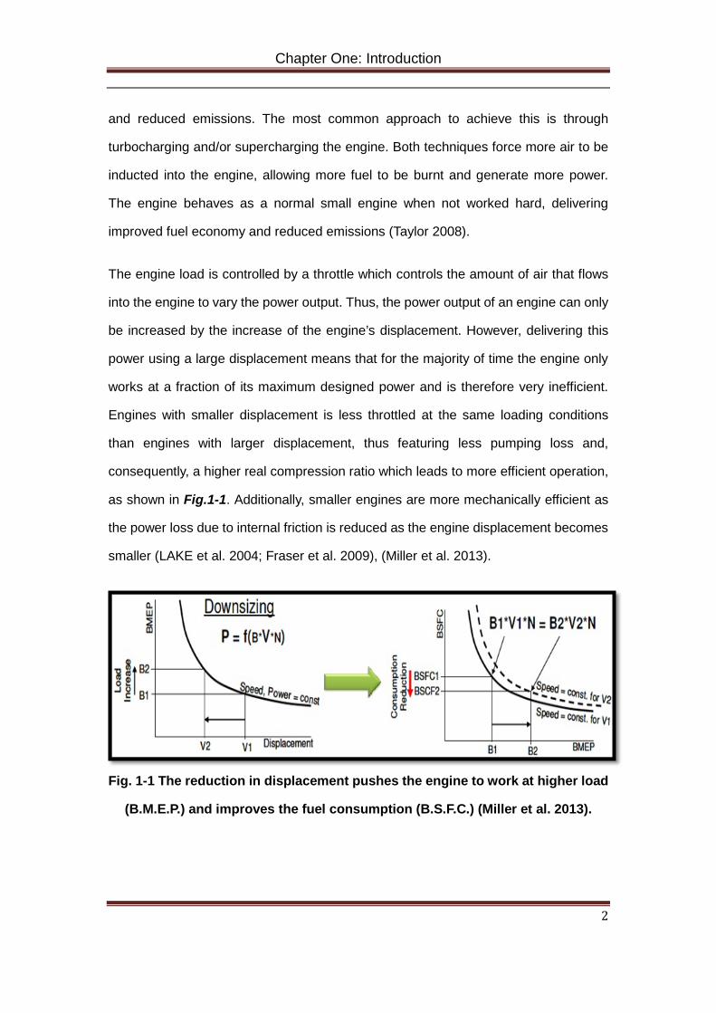
as shown in Fig.1-1. Additionally, smaller engines are more mechanically efficient as
the power loss due to internal friction is reduced as the engine displacement becomes
smaller (LAKE et al. 2004; Fraser et al. 2009), (Miller et al. 2013).
Fig. 1-1 The reduction in displacement pushes the engine to work at higher load
(B.M.E.P.) and improves the fuel consumption (B.S.F.C.) (Miller et al. 2013).
Chapter One: Introduction
3
1.1.2 Examples of downsized engines
Volkswagen 1.2 TFSI engine
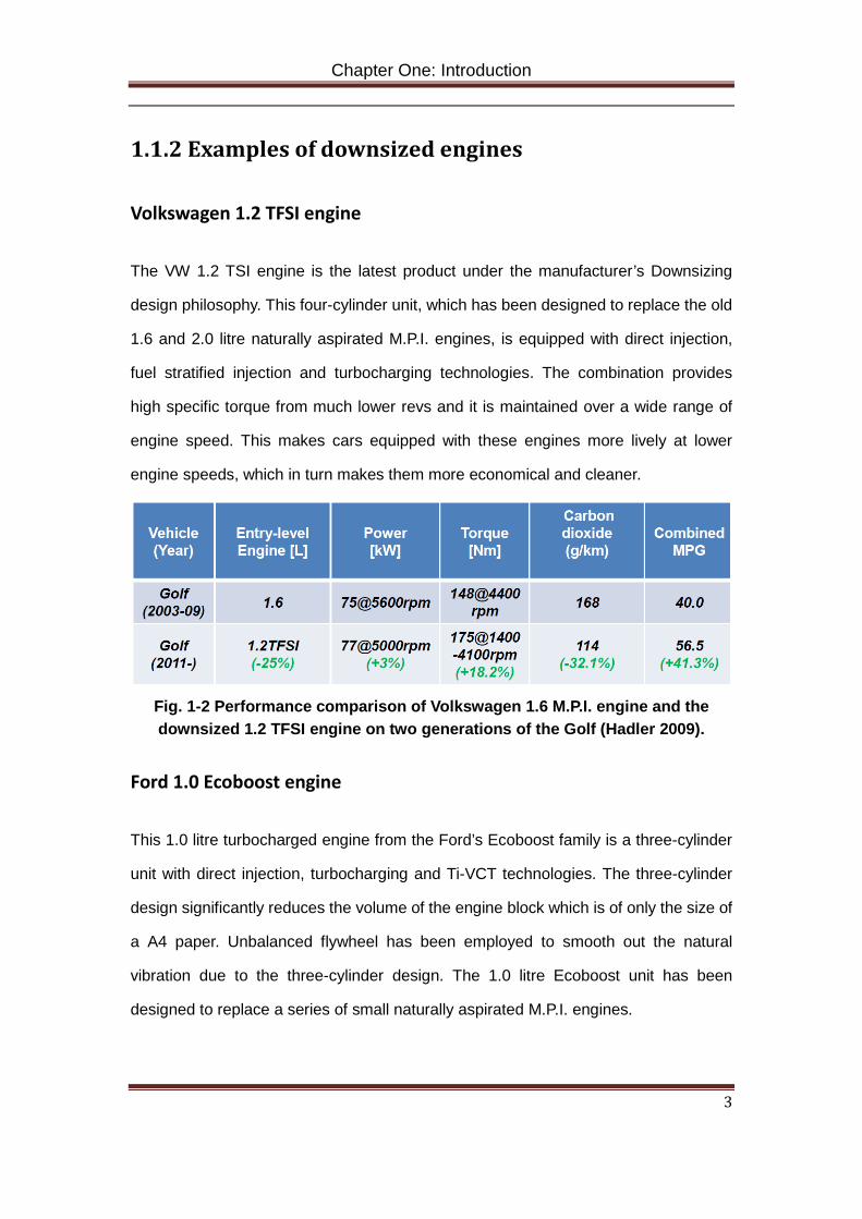
The VW 1.2 TSI engine is the latest product under the manufacturer’s Downsizing
design philosophy. This four-cylinder unit, which has been designed to replace the old
1.6 and 2.0 litre naturally aspirated M.P.I. engines, is equipped with direct injection,
fuel stratified injection and turbocharging technologies. The combination provides
high specific torque from much lower revs and it is maintained over a wide range of
engine speed. This makes cars equipped with these engines more lively at lower
engine speeds, which in turn makes them more economical and cleaner.
Fig. 1-2 Performance comparison of Volkswagen 1.6 M.P.I. engine and the downsized 1.2 TFSI engine on two generations of the Golf (Hadler 2009).
Ford 1.0 Ecoboost engine
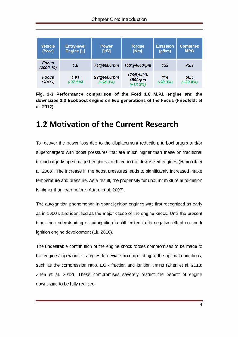
This 1.0 litre turbocharged engine from the Ford’s Ecoboost family is a three-cylinder
unit with direct injection, turbocharging and Ti-VCT technologies. The three-cylinder
design significantly reduces the volume of the engine block which is of only the size of
a A4 paper. Unbalanced flywheel has been employed to smooth out the natural
vibration due to the three-cylinder design. The 1.0 litre Ecoboost unit has been
designed to replace a series of small naturally aspirated M.P.I. engines.
Chapter One: Introduction
4
Fig. 1-3 Performance comparison of the Ford 1.6 M.P.I. engine and the downsized 1.0 Ecoboost engine on two generations of the Focus (Friedfeldt et al. 2012).
1.2 Motivation of the Current Research
To recover the power loss due to the displacement reduction, turbochargers and/or
superchargers with boost pressures that are much higher than these on traditional
turbocharged/supercharged engines are fitted to the downsized engines (Hancock et
al. 2008). The increase in the boost pressures leads to significantly increased intake
temperature and pressure. As a result, the propensity for unburnt mixture autoignition
is higher than ever before (Attard et al. 2007).
The autoignition phenomenon in spark ignition engines was first recognized as early
as in 1900’s and identified as the major cause of the engine knock. Until the present
time, the understanding of autoignition is still limited to its negative effect on spark
ignition engine development (Liu 2010).
The undesirable contribution of the engine knock forces compromises to be made to
the engines’ operation strategies to deviate from operating at the optimal conditions,
such as the compression ratio, EGR fraction and ignition timing (Zhen et al. 2013;
Zhen et al. 2012). These compromises severely restrict the benefit of engine
downsizing to be fully realized.
Chapter One: Introduction
5
During the process of autoignition, the combustible mixture of fuel and oxidizer react
in a self-accelerating manner and, eventually, ignite spontaneously leading to
combustion. The autoignition process is kinetically-controlled by the chemical chain
reactions between the fuel and the oxidizer molecules rather than any external ignition
sources. The temperature of the mixture will gradually increase and accelerate when
the energy released from chemical reactions exceeds the energy loss to the
surroundings. At a temperature that is high enough to supply the activation energy,
the reaction becomes a thermal explosion with large amount of energy being released
in a very short period of time (Liu 2010).
In spark ignition engines, autoignition occurs within the unburnt mixture ahead of the
propagating spherical flame front as a result of the piston motion and the propagating
flame front. The compression work exerted by the piston and the flame front and the
heat flux from the flame front act as external ignition sources that further raise the
unburnt mixture temperature that accelerates the unburnt mixture autoignition
process (Liu 2010). Thus it can be concluded that the temperature-sensitive
autoignition phenomenon in spark ignition engines is significantly influenced by the
flame speed and the thermal-chemical properties of the combustible mixture.
The combustion mode within spark ignition engines is turbulent premixed combustion
with a wide range of temperature and pressure variations within one cycle and from
one cycle to another (Heywood 1994). The key parameter for an accurate prediction
of the unburnt mixture temperature and pressure (and therefore the autoignition of the
unburnt mixture) is the knowledge of the turbulent flame speed throughout the
combustion process. Though a lot of efforts have been dedicated into the studies of
turbulent flame propagation in spark ignition engines, the understanding is still limited
by its transient and unsteady nature. It has been a challenge to numerically simulate
the turbulent flame speed in spark ignition engines due to the fact that it is the
outcome of the interactions between the laminar flame speed and the turbulent
Chapter One: Introduction
6
quantities, the physicochemical quantities and the external disturbances (Byun 2011).
Thus, successful calculation of the laminar flame speed is the first and the most
important step in turbulent flame speed simulations.
Laminar flame speeds of spherical flames of a fuel or fuel blends are usually acquired
experimentally using constant volume combustion bombs with sophisticated control
system and temperature and pressure measurement devices. The bomb pressure
history is used to obtained the laminar flame speed through thermodynamic analysis
(Rahim et al. 2002; Metghalchi & Keck 1982; Bradley et al. 1996; Gu et al. 2000;
Metghalchi & Keck 1980; Rozenchan et al. 2002; Kelley & Law 2009; Hu et al. 2009;
Gülder 1982; Dowdy et al. 1991; Liu et al. 2013; Verhelst et al. 2005; Iijima & Takeno
1986; Saeed & Stone 2004; Milton & Keck 1984; Lewis & von Elbe 1934; Verhelst et
al. 2011; Tang et al. 2008). The laminar flame speeds obtained in this way contain
effects of ignition and flame stretch in the initial stage of flame propagation, where the
flame radius is small. Also it includes effects of combustion bomb geometrical
confinement (if the combustion bomb is non-spherical or the flame is not ignited
centrally in a spherical combustion bomb) and flame instabilities in the later stages of
its propagation, where the flame radius is large (Burke et al. 2009). Additionally, it is
subject to relative thermal expansion all the way through the flame propagation
process (Tang et al. 2008). Due to these effects, such laminar flame speed is not as
simple as one of the fundamental properties of a specific fuel. Therefore, the
propagation mechanism of a laminar flame and its interactions with these
above-mentioned effects still need to be systematically described and numerically
characterized. Therefore the modelling of laminar flame speed should be split into two
parts. Firstly, the chemical part that deals with the combustion occurs within the
reacting flame front which is closely linked with the thermo-chemical and transport
properties of the mixture. Secondly, the part that describes the effects of flame stretch
and instabilities.
Chapter One: Introduction
7
The chemical part of laminar flame speed simulations is often ignored in available
spark ignition engine models (Heywood 1994)(Liu & Chen 2009)(Stone 1987)(Ball et
al. 1998)(Shayler et al. 1990)(Rakopoulos & Michos 2008). Instead, the combustion
and flame propagation processes are replaced by mass fraction burnt functions such
as the Wiebe functions. These models’ capabilities of combustion chemistry
simulation is limited or restricted to the use of chemical equilibrium calculations (Liu &
Chen 2009). Thus, modelling laminar flame speed in relation with chemical kinetics
provides a convenient tool for spark ignition engine simulation in terms of better
understanding of the mechanism of turbulent flame propagation and the abnormal
engine operations. Additionally, it provides the potentials of predicting the post-flame
reactions and engine-out emissions.
Chemical kinetics of fuels used in spark ignition engines has been widely studied and
can be generally interpreted as an oxidation process of fuel molecules involving a
series of complex degenerate chain branching, carrying and terminating reactions
with stable and intermediate radical species. Chemical kinetics mechanisms have
been investigated and acknowledged as an important tool in the analysis of the rates
of chemical processes and the factors that affect these rates. A chemical kinetics
mechanism contains important elementary reactions and individual species and uses
the best available rate parameters and thermo-chemical data. The size of such a
model is decided by the numbers of reactions and species included in the model,
which ranges from reduced models with only a few species and reaction steps to
detailed models consisting of hundreds of chemical species and thousands of
reactions.
The challenge arisen from using chemical kinetics in flame and engine simulations
comes from the expansive computation cost. The computational power of modern
computers has greatly advanced but is still not powerful enough to efficiently handle
chemical kinetics calculation in cooperation with multidimensional modelling. In the
Chapter One: Introduction
8
simulation of combustion in spark ignition engine simulation, the integration of
computational fluid dynamics (CFD) model with detailed chemical kinetics models,
theoretically, provides unparalleled simulation accuracy and details in presenting
combustion chamber geometries and combustion behaviour. However, numerical
modelling of this scale requires substantial computer resources. The latest
commercial IC engine simulation package that combines CFD and kinetics, the
Chemkin Fort �́� (Anon 2013), solves a complete HCCI cycle using a detailed
mechanism and 10000 mesh cells in the magnitude of 10 hours.
1.3 Aim and Objectives
The aim of the current research is, firstly, to find out how turbulent flames propagate in
naturally aspirated and boosted S.I. engines, and their interaction with the occurrence
of knock; secondly, to develop a mitigation method that depresses knock intensity at
higher intake pressure. The current study will fulfil the knowledge gap in existing SI
engine combustion models and demonstrably predicts the flame propagation process
and its relation to unburnt gas auto-ignition.
The major objectives of the current research are as follows:
1. To establish an understanding of the existing theories and modelling
philosophies of SI engine combustion and the knock phenomenon.
2. To establish an understanding of chemical kinetics and the
currently-available hydrogen- and gasoline-oxidation chemical kinetics
mechanisms.
3. To formulate a transient laminar flame speed model in a constant volume
combustion vessel to validate the philosophy of modelling transient laminar
flame speed using chemical kinetics.
Chapter One: Introduction
9
4. To establish a linkage between laminar and turbulent flame speeds using
existing theories and numerically formulate and validate a model for turbulent
flame speed a naturally aspirated SI engine.
5. Based on (4), to manipulate the input conditions and study the relation
between turbulent flame speed and the knock phenomenon. Additionally, to
develop a knock mitigation method that depresses knock while minimises
compromises on engine performance.
1.4 Outline of the Thesis
Chapter 1: Introduction
The first chapter of the thesis provides background knowledge of modern downsized
turbocharged spark ignition engines and discusses the aim, objectives and the outline
of the thesis.
Chapter 2: Literature Review
The second chapter reviews the existing modelling philosophies of spark ignition
engine combustion and the knocking phenomenon. Also included in this chapter are a
brief introduction of chemical kinetics and review and discussion of available
hydrogen- and gasoline-oxidation kinetics mechanisms.
Chapter 3: Instabilities of Spherical Hydrogen-air Flames
The third chapter introduces fundamental theories for cellular instabilities of outwardly
propagating spherical flame. Based on experimental results, discuss the effects of
temperature, pressure and equivalence ratio on the onset of cellular instabilities of
spherical hydrogen-air flames
Chapter 4: Calculation of Transient Laminar Flame Speed
The forth chapter reports a transient laminar flame speed model which consists of a
Chapter One: Introduction
10
one-dimensional three-zone thermodynamics model and an in-house chemical
kinetics solver which solves a reduced hydrogen-oxidation kinetics mechanism for the
in-flame combustion simulation. The results obtained will be validated against
experimental data.
Chapter 5: SI Engine Flame Propagation Simulation
This chapter will report the integration of the transient laminar flame speed, turbulent
flame correlation and the engine geometry model developed in previous chapters.
This integration will enable the study of flame propagation in a naturally aspirated SI
engine. Detailed descriptions of the major components and the functionality of the
numerical model will be presented. The results obtained will be validated against
available data from open literature.
Chapter 6: Downsized Boosted SI Engine Knock Simulation
This chapter will describe and discuss the effects of downsizing and turbocharging on
the flame propagation and its relation to the unburnt gas auto-ignition and, potentially,
the knocking phenomenon.
Chapter 7: SI Engine Knock Mitigation
This chapter discuss a SI engine knock mitigation strategy that supress the knock
while minimises the compromises on engine performance.
Chapter 8: Conclusions and Future Work
The final chapter of the thesis will discuss and conclude the achievements and the
deficiencies of the current research work. Future work that can be done to improve the
current work will be suggested.
Chapter Two: Literature Review
11
Chapter Two: Literature Review
2.1 SI Engine Combustion
In S.I. engines with a conventional pan-shaped combustion chamber, the turbulence
is mostly generated by the high shear flows during the induction process and modified
during the compression. It is well established that the turbulence intensity as well as
the mean flow increases almost in a linear fashion with increasing engine speed
(Daneshyar & Hill 1987). The turbulence decays rapidly towards the end of the
induction process and the characteristic dissipation time for the turbulent kinetic
energy is smaller than the engine time scales. The turbulence during the induction
exhibits a strong anisotropy, and the turbulence intensity as well as the mean velocity
shows significant spatial variations. For disc shaped chambers, the turbulence when
averaged over several cycles, displays a homogeneous and more isotropic structure
towards the end of the compression stroke for both swirling and non-swirling flows
(Gülder & Smallwood 2001).
As shown in Fig. 2-1, it is widely accepted that the combustion regime in premixed SI
engines falls into the wrinkled flame regime (Gülder & Smallwood 2001) and such
conclusion is supported by extensive experimental results. By using molecular
Rayleigh scattering, one researcher (Keck 1982) found that the flame front in spark
ignition engines is made up of wrinkled laminar flames and islands of unburnt mixture
may appear occasionally. For low-intensity large-scale turbulence, Damkohler (1947)
proposed that ST/SL, the ratio of the turbulent burning velocity (ST) to the laminar
burning velocity (SL), is proportional to Aw/Ao, the ratio of the wrinkled flame surface
area (Aw) to the flow cross section area (Ao). For high-intensity, small- scale
Chapter Two: Literature Review
12
turbulence, combustion takes place in a distributed manner rather than a front
propagation. Williams (1985) further claimed that, under the wrinkled turbulent
combustion regimes, the process can be separated from the turbulence. Therefore, it
is feasible to study the turbulent combustion process as a combination of two distinct
phenomena: laminar flame propagation and turbulent flow field.
2.1.1 Regimes of SI Engine Combustion
In Fig. 2-1 premixed turbulent combustion is classified into several regimes according
to velocities, length scale and a number of dimensionless parameters (Peters 2000).
Several scales can be defined in the study of turbulence. The integral time scale, 𝝉𝒕,
associated with energy dissipation of large eddies is defined as:
𝝉𝒕 = 𝒍𝒕𝒖𝒕′
(2-1)
𝒍𝒕 = 𝑪𝑫𝒖𝒕′
𝟑
∈ (2-2)
where 𝒍𝒕 is the integral length scale of the large energy-containing eddies, 𝒖𝒕′ is the
r.m.s turbulent velocity and 𝑪𝑫 is the turbulent length scale constant. The chemical
time scale, 𝝉𝒄, is defined as:
𝝉𝒄 = 𝜶𝑺𝑳
𝟐 ; 𝜶 = 𝒌𝝆𝑪𝒑
(2-3)
where 𝜶 is the thermal diffusivity and 𝒌 is the thermal conductivity. The smallest
eddies in a turbulent flow are characterized by the Kolmogorov time, velocity, and
length scales:
𝝉𝜼 = (𝝊𝝐)𝟏/𝟐; 𝝂𝜼 = (𝝊𝝐)𝟏/𝟒; 𝜼 = (𝝂
𝟑
𝝐)𝟏/𝟒 (2-4)
Some dimensionless parameters can be defined from above-mentioned time and
length scales. These parameters are used to distinguish different combustion
Chapter Two: Literature Review
13
regimes.
Turbulence Reynolds Number (𝑹𝑹𝒕):
𝑹𝑹𝒕 = 𝐮𝐭′𝐥𝐭𝛎
(2-5)
The turbulence Reynolds number characterises a turbulent flow in terms of the
turbulence RMS velocity, 𝐮𝐭′. It represents the ratio between the inertia force and the
viscous force of the flow.
Damkohler Number (𝑫𝑫):
𝑫𝑫 = 𝝉𝒕𝝉𝒄
(2-6)
The Damkohler number represents the ratio between the turbulence time scale and
the chemical time scale. It indicates which one of these two effects is more dominant.
Karlovitz Number (Ka):
𝑲𝑫 = 𝝉𝒄𝝉𝜼
(2-7)
It defines the ratio of the chemical time scale and the Kolmogorov scale. When
𝑲 ≪ 𝟏 the chemical reactions occur much faster than all turbulent scales.
Turbulence does not alter the flame structure and the chemical region is laminar.
Prandlt Number (Pr):
𝑷𝑷 = 𝝂𝜶 (2-8)
The Prandlt number represents the ratio between the viscous force and the thermal
diffusivity. It can related to the thickness of the thermal and velocity boundary layers.
Lewis Number (Le):
𝑳𝑹 = 𝜶𝑫 (2-9)
The Lewis number is the ratio between the thermal and molecular diffusivity of a
species.

Chapter Two: Literature Review
14
Fig. 2-1 Illustration of regimes of turbulent premixed combustion. The rectangle
identifies the regimes of SI engines (Heywood 1988).
Chapter Two: Literature Review
15
2.1.2 SI Engine Modelling
Multi-dimensional CFD models
Multidimensional modelling has been adopted as a powerful tool to investigate and
analyse phenomena occurring in internal combustion engines, particularly with the
rapid increase of computer power in recent years. Theoretically, a full-scale
integration of CFD model of fine grid design with detailed chemical kinetics model
provides unrivalled simulation accuracy and details of in-cylinder flow and combustion
behaviours. However, a model at this numeric scale requires substantial CPU
computing speed, large-scale storage and robust and fast numerical algorithm. Even
with today’s advanced high performance computers, the simulation time of such
models is still measured in weeks or months.
Several solutions have been proposed trying to find the balance between the
computational costs and the simulation accuracy. Reitz et al. (2006) adopted a
7-species chemical equilibrium model into his multi-dimensional engine model. The
turbulent flame location, local temperature and pressure and the heat release rate are
computed using KIVA-3V CFD codes with a mesh size in the range of 2-5mm. Burnt
products are assumed to reach thermodynamic and chemical equilibrium states
immediately behind the flame brush.
Other researchers proposed cost-reduction solution methods that either adopted a
global or reduced chemical kinetics mechanism (Li et al. 2003; Kong & Reitz 1993; Ali
et al. 2003) or a reduced CFD mesh to one- or two-dimensional (Iida et al. 2003;
Iwashiro et al. 2002). These methods suffer from either degraded simulation accuracy
or computational costs that are still relatively high.
Aceves et al. (2000) was among the first researchers who presented hybrid approach
that formed a segregated sequential CFD multi-zone thermo-kinetic model. In the
Chapter Two: Literature Review
16
model, a detailed chemical kinetics model is implemented into a KIVA-2.1 CFD solver
and a multi-zone thermodynamics model. The CFD model is responsible for solving
the temperature and mixture formation process in the compression stroke until the
ignition timing. The multi-zone model takes over from the ignition and simulates the
combustion and expansion processes. These zones are defined by mass distribution
and mixing between adjacent zones is disallowed. The model was validated against
experimental results and showed good capability of predicting cylinder pressure and
burn rate. The model also successfully reduced the computation time scale from
weeks or months to hours or days. However, the model failed on the prediction of HC
and CO emissions which are critical in modern engine design.
Quasi-dimensional multi-zone models
Quasi-dimensional models are used to simulate the ‘closed’ part of the S.I. engine
cycle as they cannot properly predict the intake and exhaust strokes due to their
dimensionless nature (Verhelst & Sheppard 2009). Quasi-dimensional models are
distinguished from zero-dimensional models by the inclusion of certain geometrical
parameters in the basic thermodynamic approach. This usually includes the radius of
a thin flame front that separates the burnt and unburnt zones, creating a two-zone
formation.
One advantage of these zero-dimensional models is the avoidance of the modelling of
the in-cylinder process. Instead of considering the intake, mixture preparation,
combustion and exhaust processes, a zero-dimensional model uses a pre-defined
mass burning rate, also known as the Wiebe function (Liu & Chen 2009), to describe
the combustion process. When the engine operating point stays the same Wiebe
functions provide unrivalled simulation accuracy as it, in fact, works back from known
experimental results. However as each Wiebe function is empirically defined as a
specific engine operating point, extrapolation to other operating points is problematic.
Chapter Two: Literature Review
17
Most quasi-dimensional S.I. engine models adopt a two-zone formation, assuming
that the flame is a ultimately thin transition layer that transport mass and energy
between the burnt and unburnt zones (Liu & Chen 2009). Additionally, the flame is
assumed to be adiabatic and in chemical and thermodynamic equilibrium. The
unburnt mass entrained into the flame is assumed to be consumed and transferred
into burnt mass instantaneously. The burnt mixture composition is calculated using
chemical equilibrium at a pre-defined combustion temperature and pressure. Typically,
up to 12 species are considered in the equilibrium calculation: H2O, H2, OH, H, N2,
NO, N, CO2, CO, O2, O and Ar (Verhelst & Sheppard 2009). The actual number of
species considered varies when the interests of the simulation shifts from just the
combustion process. Reitz et al. (2006) used a 7-species chemical equilibrium system
to determine the burnt mixture composition but an additional 10-species and
9-reaction kinetics model was adopted to predict the formation of NO and NO2. Liu et
al. (2009) proposed an zero-dimensional two-zone model to study the knock in S.I.
engine. A chemical equilibrium containing 32 species was used in Liu’s model. The
larger equilibrium system was chosen in order to keep accordance to the number of
species included in the reduced chemical kinetics mechanism used to predict end gas
autoignition.
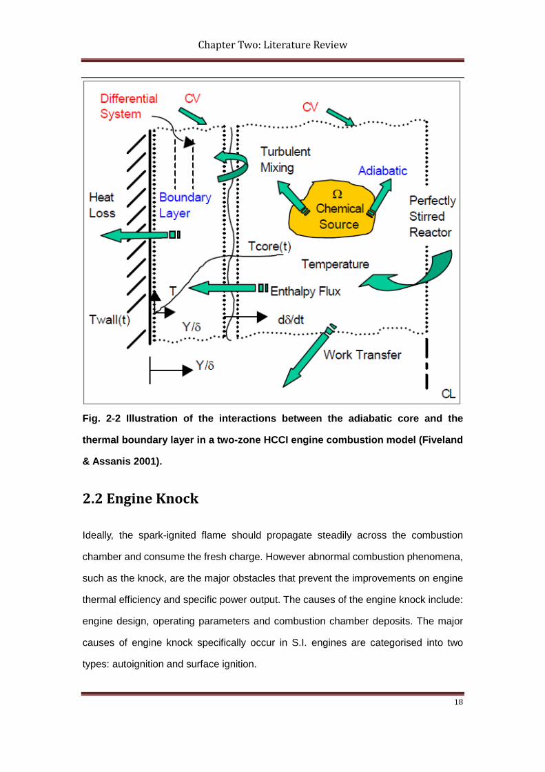
In additional to the two-zone layout, some researchers developed a thermal boundary
layer between the unburnt zone and the cylinder wall (Fiveland & Assanis 2001;
Puzinauskas & Borgnakke 1991; Borgnakke et al. 1980), as shown in Fig. 2-2. The
addition of the boundary layer aids the fundamental understanding of the heat transfer
process inside the cylinder.
Chapter Two: Literature Review
18
Fig. 2-2 Illustration of the interactions between the adiabatic core and the
thermal boundary layer in a two-zone HCCI engine combustion model (Fiveland
& Assanis 2001).
2.2 Engine Knock
Ideally, the spark-ignited flame should propagate steadily across the combustion
chamber and consume the fresh charge. However abnormal combustion phenomena,
such as the knock, are the major obstacles that prevent the improvements on engine
thermal efficiency and specific power output. The causes of the engine knock include:
engine design, operating parameters and combustion chamber deposits. The major
causes of engine knock specifically occur in S.I. engines are categorised into two
types: autoignition and surface ignition.
Chapter Two: Literature Review
19
2.2.1 Autoignition
The combustion process in modern S.I. engines is precisely controlled by the spark
ignition timing towards the end of the compression stroke. A flame kernel is formed a
few milliseconds after the spark is fired. The flame kernel continues to grow outwardly
and becomes a self-sustainable turbulent flame. The turbulent flame propagate
across the combustion chamber to gradually consume the combustible fresh charge.
As the flame propagates across combustion chamber the end gas is compressed by
the flame front and the upward motion of the piston, causing pressure, temperature
and density to increase. Some of the end gas fuel-air mixture may undergo slower
pre-flame chemical reactions and start to release heat energy. This phenomenon is
generally termed as ‘Autoignition’ (Heywood 1988). The autoignited end gases then
burn very rapidly releasing energy at a rate 5 to 25 times higher in comparison to
normal combustion. The occurrence of end gas autoignition depends on the
competition between the consumption rate of the turbulent flame and the pre-flame
chemical reactions ahead of the flame. If the end gas that has already autoignited is
not consumed by the flame before the chemical reactions proceed to a critical level,
sharp local temperature and pressure increase will occur (Liu 2010).
A sonic pressure wave is then created by the autoignition and it spreads across and
resonates in the combustion chamber. This causes high frequency pressure
oscillations inside the cylinder that produce sharp metallic noise and excessive
vibration to the engine block. Such manifestations are termed as the knock. Knock is
undesirable as high pressure and local temperature can cause severe engine
damage and is unpleasant to the driver and the passengers of the car. Fig. 2-3
illustrates normal combustion and knocking combustion processes of S.I. engines. It
has been acknowledged that knock is most likely to occur under high engine load at
low engine speed. High engine load generates high cylinder temperature and
pressure which triggers the end gas autoignition. Low engine speed allows the
Chapter Two: Literature Review
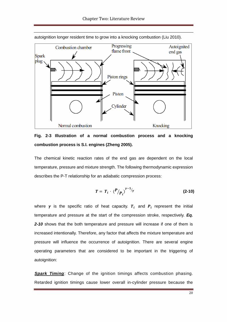
20
autoignition longer resident time to grow into a knocking combustion (Liu 2010).
Fig. 2-3 Illustration of a normal combustion process and a knocking
combustion process is S.I. engines (Zheng 2005).
The chemical kinetic reaction rates of the end gas are dependent on the local
temperature, pressure and mixture strength. The following thermodynamic expression
describes the P-T relationship for an adiabatic compression process:
𝑻 = 𝑻𝒊 ∙ (𝑷 𝑷𝒊� )𝜸−𝟏
𝜸� (2-10)
where 𝜸 is the specific ratio of heat capacity. 𝑻𝒊 and 𝑷𝒊 represent the initial
temperature and pressure at the start of the compression stroke, respectively. Eq.
2-10 shows that the both temperature and pressure will increase if one of them is
increased intentionally. Therefore, any factor that affects the mixture temperature and
pressure will influence the occurrence of autoignition. There are several engine
operating parameters that are considered to be important in the triggering of
autoignition:
Spark Timing : Change of the ignition timings affects combustion phasing.
Retarded ignition timings cause lower overall in-cylinder pressure because the
Chapter Two: Literature Review
21
combustion phasing is shifted away from the TDC position, which leads to the main
combustion with major heat release occurs within a larger and faster expanding
volume as the piston is moving downward. As a contrast, advanced spark timings
causes earlier combustion that results in higher cylinder pressures. Knock
occurrence is more subject to earlier spark timings because of the maximum end-gas
temperature is increased.
Compression Ratio: With increased compression ratios, the volume swept by the
piston during the compression and combustion phases becomes smaller. This leads
to more intense compression on the end-gas and higher heat release from the mixture.
As a result, a higher compression ratio increases the cylinder pressure and end gas
temperatures.
Air-Fuel Ratio: At different AFRs, the in-cylinder mixture shows different combustion
strength. Change of the mixture composition and thermodynamic properties affects
combustion rates and the energy release, which in turn affects the cylinder pressure
and the end-gas temperatures.
Intake Pressure: A higher intake pressure forces a larger amount of air-fuel mixture
into the cylinder with higher initial pressure and volumetric efficiency cylinder, which
consequently leads to higher overall in-cylinder pressure and combustion
temperature.
Intake Temperature: It can be deduced from Eq. 2-1 that mixture temperature in the
compression process scales closely with initial temperature. Higher initial
temperatures lead to higher overall mixture temperatures throughout the compression
and combustion processes, which promote the rates of autoignition reactions.
EGR: Using EGR increases the total heat capacity of the end-gas and consequently
reduces the temperature rise of the gas, which thermally diminishes knock tendency.
However, the large number of reactive species present in the exhaust gas can also
Chapter Two: Literature Review
22
promote autoignition by chemical means.
Engine Speed: The chemical reactions of the end-gas takes time to proceed. At lower
engine speeds, flame propagating speed become equivalent to or slower than the
reaction characteristic time, so autoignition reactions is more likely to build up and
advance.
Charge Preparation: The flow dynamic motion (turbulence, swirl, and tumble) affects
the homogeneity of the mixture, which has a significant effect on combustion process.
Local inhomogeneity of the mixture could lead to incomplete combustion or regionally
high combustion temperature.
Combustion Chamber Geometry: The general shape of the combustion chamber,
as well as spark plug location, affects the flame front area and the distance the flame
front travels. Longer flame travel distance results in longer combustion duration and
more time for autoignition chemistry to proceed.
2.2.2 Surface Ignition
Surface ignition describes the phenomena when the unburnt mixture is ignited by the
overheated components in the cylinder or by glowing deposits. Those overheated
components are typically the exhaust valves and the spark plug. Typical examples of
glowing deposits can be carbon deposits and hot engine oil droplets (Dahnz et al.
2010). Surface ignition can occur before the spark ignition (pre-ignition) or after the
spark ignition (post-ignition). Surface ignition creates one or multiple propagating
flame fronts which interact with the main flame front to generate knocking combustion.
The knock induced by surface ignition may be more intense than that induced by end
gas autoignition. The reason being that multiple flame fronts can be ignited by the
glowing deposits very early in the compression stroke and lead to more rapid heat
release and rises of cylinder temperature and pressure (Heywood 1988). The knock
Chapter Two: Literature Review
23
originated from surface ignition cannot be controlled or mitigated effectively by the
methods mentioned above.
2.2.3 The knock models
The modelling of end gas autoignition consists of two major categories: empirical
correlations and chemical kinetics modelling (Heywood 1988). The experimental
methods and empirical correlations are used to study end gas autoignition when the
fundamental understanding of the chemistry involved were incomplete. Over the
years, chemical kinetics modelling attracts more and more attention in the study of
end gas autoignition, thanks to both improved understanding of autoignition chemistry
and greatly advanced computational power. Numerical modelling provides a simple
and cost-effective way of study end gas autoignition, compared to experimental
methods.
Empirical correlations
The empirical expression for autoignition is derived by matching an Arrhenius function
to measured data obtained from ignition delay time experiments. For a given
fuel-oxidizer mixture under the conditions of P and T, the ignition delay time is
expressed as:
𝝉 = 𝑨 ∙ 𝑷−𝒏 ∙ 𝑬𝑬𝑷(𝑩 𝑻⁄ ) (2-11)
where A and B are fitting parameters dependent on fuel types and are obtained based
on experimental results. A reaction progress coefficient, c, is integrated to predict the
occurrence of knock with temporal histories of temperature and pressure (Bray et al.
1994). Autoignition is deemed to occur when 𝝉 exceeds a threshold value. Douaud
and Eyzat (1978) proposed a correlation that has been extensively tested and widely
accepted:
Chapter Two: Literature Review
24
𝒄 = 𝟏𝟏.𝟔𝟔 ∙ (𝑶𝑶𝟏𝟏𝟏
)𝟑.𝟒𝟏𝟐 ∙ 𝑷−𝒏 ∙ 𝑬𝑬𝑷(𝟑𝟔𝟏𝟏 𝑻⁄ ) (2-12)
where 𝝉 is the induction time in milliseconds and ON is the octane number of the fuel.
Empirical autoignition correlations in this form can be used in S.I. engine models.
Although the correlations, by their own, are extensively tested, their ability of
accurately predicting knock is still unclear in practice. Additionally, these correlations
are too simple to prove any information on the reaction process.
Chemical kinetics modelling
The autoignition is a complex chemical process that involves hundreds of species and
thousands of elementary reactions. Autoignition of simpler fuels, e.g. hydrogen, may
include around 10 species and 20 reactions (O Conaire et al. 2004), while that of
heavy hydrocarbon fuels, e.g. n-heptane, can contain more than 500 species and
3000 reactions (Curran et al. 1998).
In order to obtain complete predictions of any autoignition process, one should have
all the reaction rate constants and elementary reaction steps in hand and powerful
computational resource at acceptable cost. At the present time none of the above two
requirement is fulfilled: the understanding of the elementary steps and rate constants
is still lacking, the high performance computers are too costly to be widely used.
However, chemical kinetics modelling has still been greatly advanced in the past a
few decades and is becoming an essential tool in the design and research of
combustion systems. Westbrook and Dryer (1984) attributed the advancement of
chemical kinetics modelling to the following factors:
1. Larger amount of elementary kinetic data becomes available.
2. Improvement in reaction rates estimation.
Chapter Two: Literature Review
25
3. Development of faster and more reliable numeric algorithms.
4. Continuous advancement of computers
More information with regards to chemical kinetics and its applications in hydrogen
and hydrocarbon oxidation studies is available in later chapters.
2.3 Laminar flames
Laminar flames are of great importance in the study of IC engine combustion.
Premixed laminar flames can be adequately described by precise definitions of the
following aspects: inner flame structures; flame thickness; dynamics of flame and
flame stretch (Groot 2003).
2.3.1 Laminar flame structure
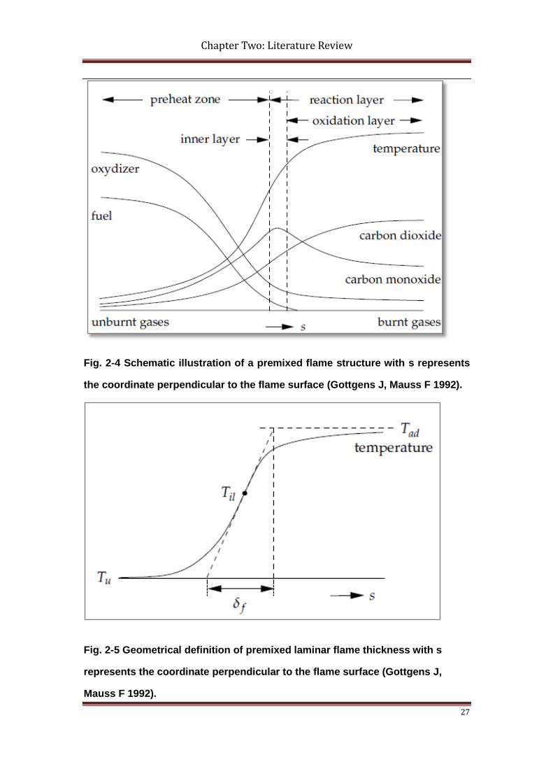
According to the temperature and species concentration gradients, a premixed flame
can be considered to consist of three distinctive layers: the pre-heat layer, the inner
layer and the oxidation layer, as shown in Fig. 2-4. During combustion the flame acts
as a conversion layer that lies between the unburnt zone, where a large amount of
fuel and oxidiser present, and the burnt zone, whereas the amount is significantly
reduced. In the detailed structure of a flame, the temperature increases smoothly from
the initial in the pre-heat zone to its final state inside the oxidation layer. The
concentrations of the intermediates and products will change in a similar manner,
whereas the concentrations of fuel and oxidiser show a significant decrease.
The pre-flame layer refers to the unburnt mixtures that are immediately upstream of
the inner layer. Chemical reactions within this layer proceed with very slow reaction
rates and can be considered as chemically inert. The unburnt mixture is heated up by
the heat flux from the reaction layer. In general, the pre-flame zone can be seen as a
mixture preparation zone for the reaction layer.
Chapter Two: Literature Review
26
The reaction zone is further divided into two sub-layers: the inner layer and the
oxidation layer. In the inner layer, or often referred as fuel-consumption layer, fuel is
consumed and converted into hydrogen and carbon monoxide, and active radicals are
depleted by chain-breaking reactions. The inner layer makes most of the visible part
of the flame and the visibility is due to those electronically-excited light-emitting
species, such as CH, CN, C2, and CHO, returning to their ground state. The inner
layer is the thinnest compared to pre-flame layer and oxidation layer, typically by the
order of one fifth to one tenth (Peters 1991). Majority of the energy is released within
the inner layer and therefore the temperature gradient within the inner layer is the
sharpest amongst the three layers. The combustion intermediates hydrogen and
carbon monoxide reach their maximum concentrations within the inner layer.
The oxidation layer is located downstream of the reaction layer. Within the oxidation
layer carbon monoxide and hydrogen are further oxidised into carbon dioxide and
water. Thermodynamic equilibrium of all species is established in the oxidation layer
rather than the inner layer as the residual time is not sufficient. Chemical reactions
occur in the oxidation layer are often referred to as post-flame reactions and they play
an important role in the products formation and the overall heat release of the
combustion.
2.3.2 Laminar flame thickness
Flame thickness is an important scale parameter of any premixed laminar flames that
it represents the depth of the reaction zone in which the fuel is consumed and bulk of
heat is released. A classical definition of flame thickness δf is based on a geometrical
approach, as shown in Fig. 2-5. In this case, the thickness is defined as the interval of
the steepest tangent to the temperature profile between the unburnt temperature and
the adiabatic flame temperature (Heywood 1988):
𝜹𝒇 = 𝑻𝑫𝒂−𝑻𝒖(𝒂𝑻/𝒂𝒅)𝑻𝒊𝒍
(2-13)
Chapter Two: Literature Review
27
Fig. 2-4 Schematic illustration of a premixed flame structure with s represents
the coordinate perpendicular to the flame surface (Gottgens J, Mauss F 1992).
Fig. 2-5 Geometrical definition of premixed laminar flame thickness with s
represents the coordinate perpendicular to the flame surface (Gottgens J,
Mauss F 1992).
Chapter Two: Literature Review
28
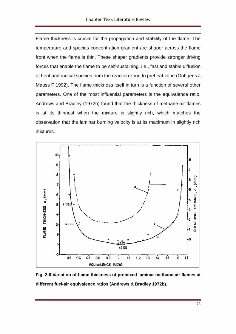
Flame thickness is crucial for the propagation and stability of the flame. The
temperature and species concentration gradient are shaper across the flame
front when the flame is thin. These shaper gradients provide stronger driving
forces that enable the flame to be self-sustaining, i.e., fast and stable diffusion
of heat and radical species from the reaction zone to preheat zone (Gottgens J,
Mauss F 1992). The flame thickness itself in turn is a function of several other
parameters. One of the most influential parameters is the equivalence ratio.
Andrews and Bradley (1972b) found that the thickness of methane-air flames
is at its thinnest when the mixture is slightly rich, which matches the
observation that the laminar burning velocity is at its maximum in slightly rich
mixtures.
Fig. 2-6 Variation of flame thickness of premixed laminar methane-air flames at
different fuel-air equivalence ratios (Andrews & Bradley 1972b).
Chapter Two: Literature Review
29
2.3.3 Laminar burning velocity
The laminar burning velocity, denoted as 𝒖𝑳, is one of the most fundamental and
important properties of premixed flames. It can be defined as the velocity at which a
flame front moves in the normal direction to its surface into the adjacent unburnt
mixture due to chemical reactions and the diffusion of heat and mass (Groot 2003).
Previous research on laminar burning velocities of various fuels revealed that there
are a few dominating parameters that strongly influence the laminar burning velocity
(Iijima & Takeno 1986; Liu et al. 2013; Metghalchi & Keck 1982; Bradley et al. 1996;
Dowdy et al. 1991; Gu et al. 2000; Gülder 1982; Hu et al. 2009a; Metghalchi & Keck
1980; Milton & Keck 1984; Rahim et al. 2002):
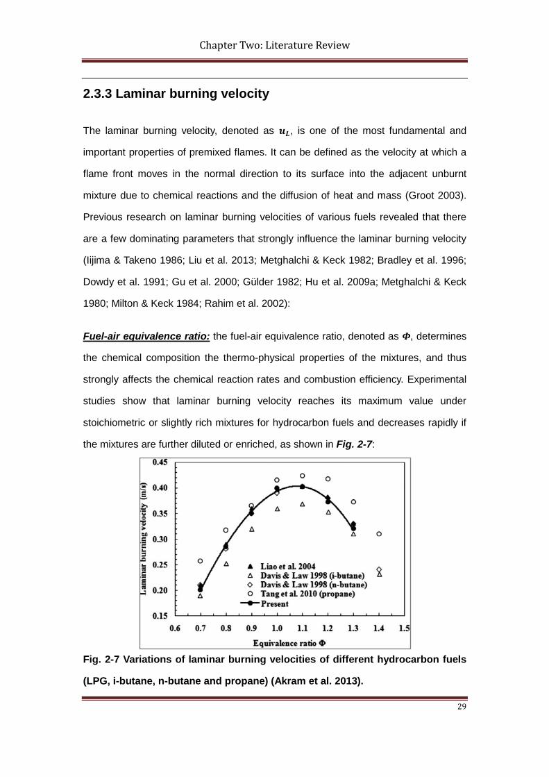
Fuel-air equivalence ratio: the fuel-air equivalence ratio, denoted as Ф, determines
the chemical composition the thermo-physical properties of the mixtures, and thus
strongly affects the chemical reaction rates and combustion efficiency. Experimental
studies show that laminar burning velocity reaches its maximum value under
stoichiometric or slightly rich mixtures for hydrocarbon fuels and decreases rapidly if
the mixtures are further diluted or enriched, as shown in Fig. 2-7:
Fig. 2-7 Variations of laminar burning velocities of different hydrocarbon fuels
(LPG, i-butane, n-butane and propane) (Akram et al. 2013).
Chapter Two: Literature Review
30
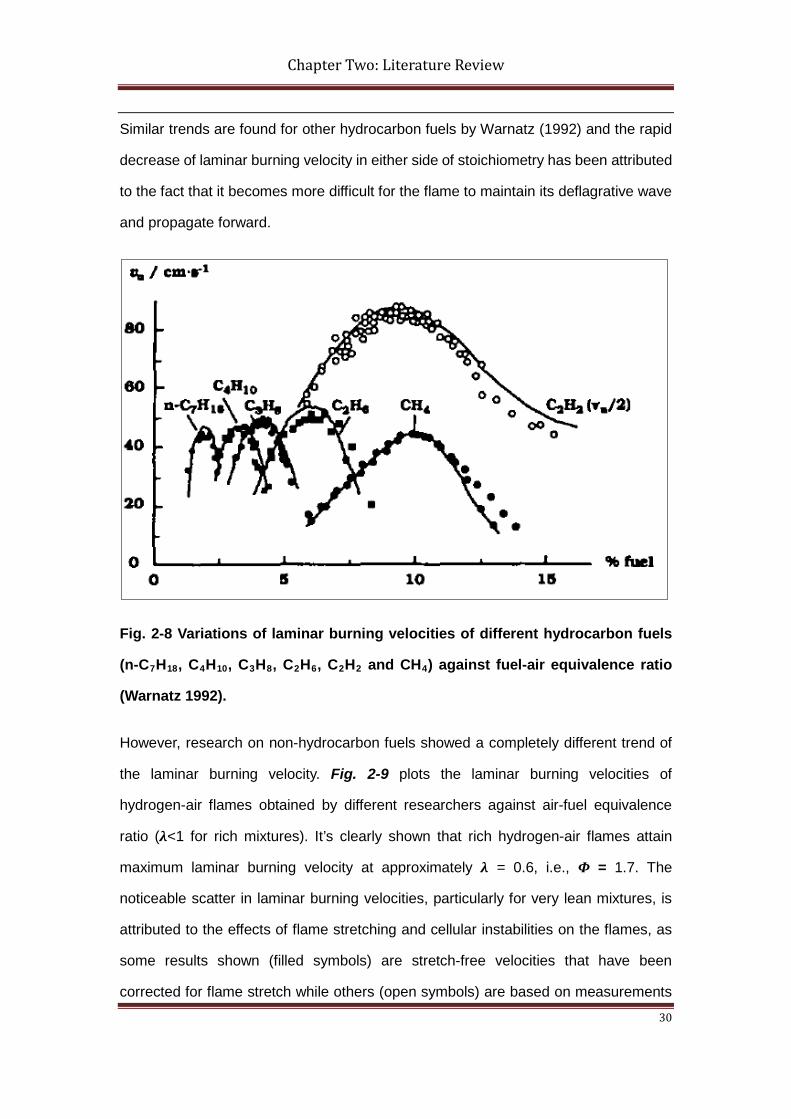
Similar trends are found for other hydrocarbon fuels by Warnatz (1992) and the rapid
decrease of laminar burning velocity in either side of stoichiometry has been attributed
to the fact that it becomes more difficult for the flame to maintain its deflagrative wave
and propagate forward.
Fig. 2-8 Variations of laminar burning velocities of different hydrocarbon fuels
(n-C7H18, C4H10, C3H8, C2H6, C2H2 and CH4) against fuel-air equivalence ratio
(Warnatz 1992).
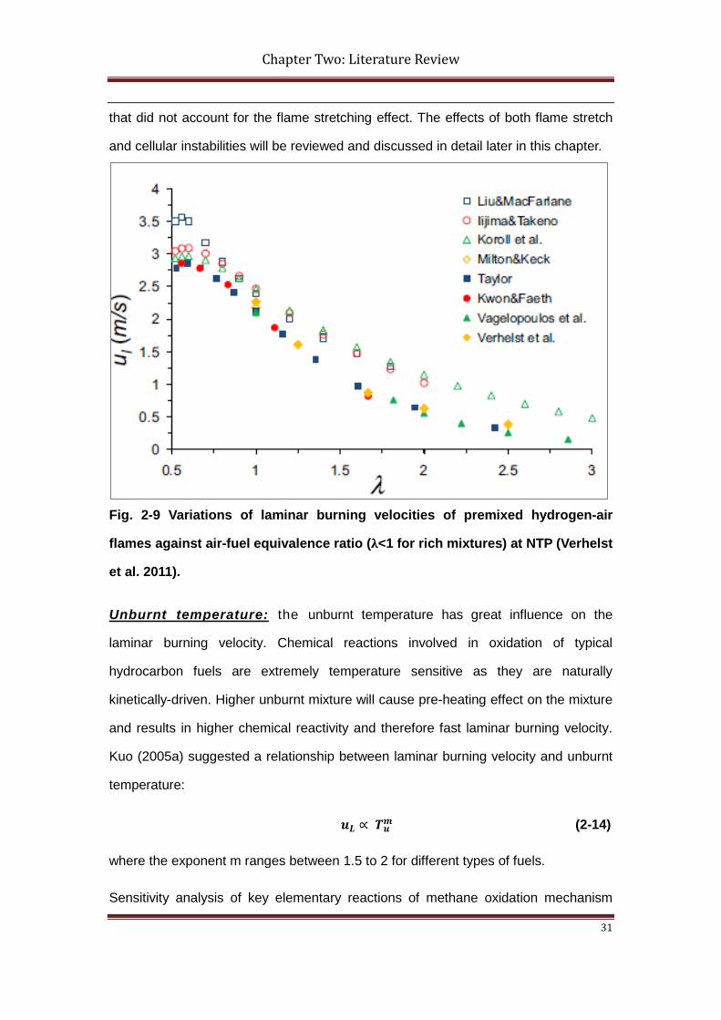
However, research on non-hydrocarbon fuels showed a completely different trend of
the laminar burning velocity. Fig. 2-9 plots the laminar burning velocities of
hydrogen-air flames obtained by different researchers against air-fuel equivalence
ratio (λ<1 for rich mixtures). It’s clearly shown that rich hydrogen-air flames attain
maximum laminar burning velocity at approximately λ = 0.6, i.e., Ф = 1.7. The
noticeable scatter in laminar burning velocities, particularly for very lean mixtures, is
attributed to the effects of flame stretching and cellular instabilities on the flames, as
some results shown (filled symbols) are stretch-free velocities that have been
corrected for flame stretch while others (open symbols) are based on measurements
Chapter Two: Literature Review
31
that did not account for the flame stretching effect. The effects of both flame stretch
and cellular instabilities will be reviewed and discussed in detail later in this chapter.
Fig. 2-9 Variations of laminar burning velocities of premixed hydrogen-air
flames against air-fuel equivalence ratio (λ<1 for rich mixtures) at NTP (Verhelst
et al. 2011).
Unburnt temperature: the unburnt temperature has great influence on the
laminar burning velocity. Chemical reactions involved in oxidation of typical
hydrocarbon fuels are extremely temperature sensitive as they are naturally
kinetically-driven. Higher unburnt mixture will cause pre-heating effect on the mixture
and results in higher chemical reactivity and therefore fast laminar burning velocity.
Kuo (2005a) suggested a relationship between laminar burning velocity and unburnt
temperature:
𝒖𝑳 ∝ 𝑻𝒖𝒎 (2-14)
where the exponent m ranges between 1.5 to 2 for different types of fuels.
Sensitivity analysis of key elementary reactions of methane oxidation mechanism
Chapter Two: Literature Review
32
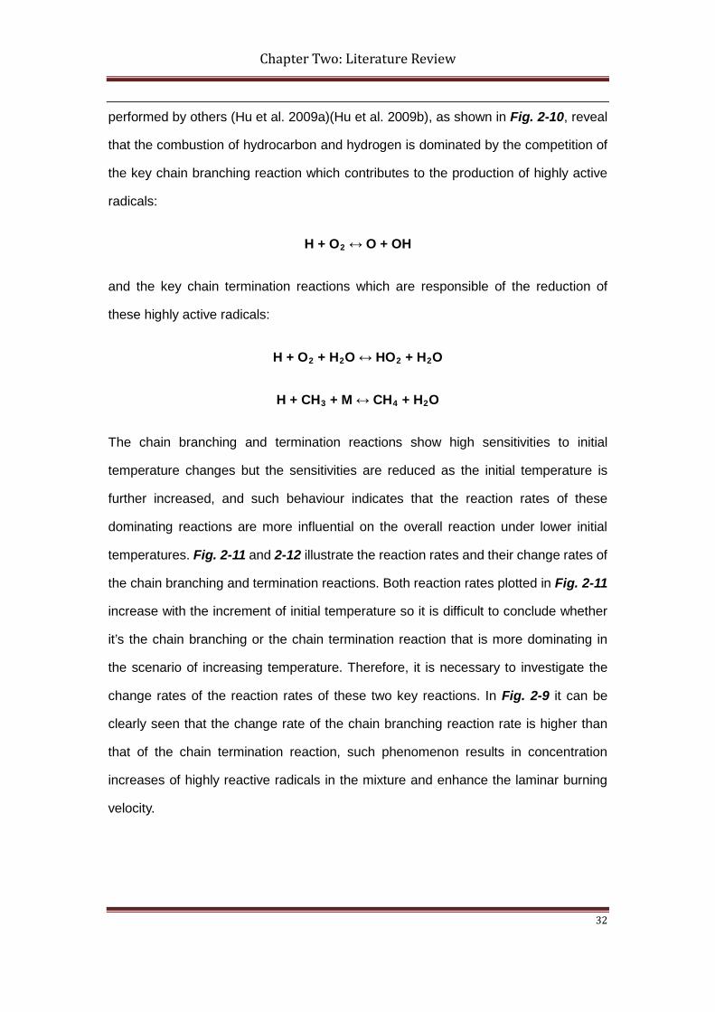
performed by others (Hu et al. 2009a)(Hu et al. 2009b), as shown in Fig. 2-10, reveal
that the combustion of hydrocarbon and hydrogen is dominated by the competition of
the key chain branching reaction which contributes to the production of highly active
radicals:
H + O2 ↔ O + OH
and the key chain termination reactions which are responsible of the reduction of
these highly active radicals:
H + O2 + H2O ↔ HO2 + H2O
H + CH3 + M ↔ CH4 + H2O
The chain branching and termination reactions show high sensitivities to initial
temperature changes but the sensitivities are reduced as the initial temperature is
further increased, and such behaviour indicates that the reaction rates of these
dominating reactions are more influential on the overall reaction under lower initial
temperatures. Fig. 2-11 and 2-12 illustrate the reaction rates and their change rates of
the chain branching and termination reactions. Both reaction rates plotted in Fig. 2-11
increase with the increment of initial temperature so it is difficult to conclude whether
it’s the chain branching or the chain termination reaction that is more dominating in
the scenario of increasing temperature. Therefore, it is necessary to investigate the
change rates of the reaction rates of these two key reactions. In Fig. 2-9 it can be
clearly seen that the change rate of the chain branching reaction rate is higher than
that of the chain termination reaction, such phenomenon results in concentration
increases of highly reactive radicals in the mixture and enhance the laminar burning
velocity.
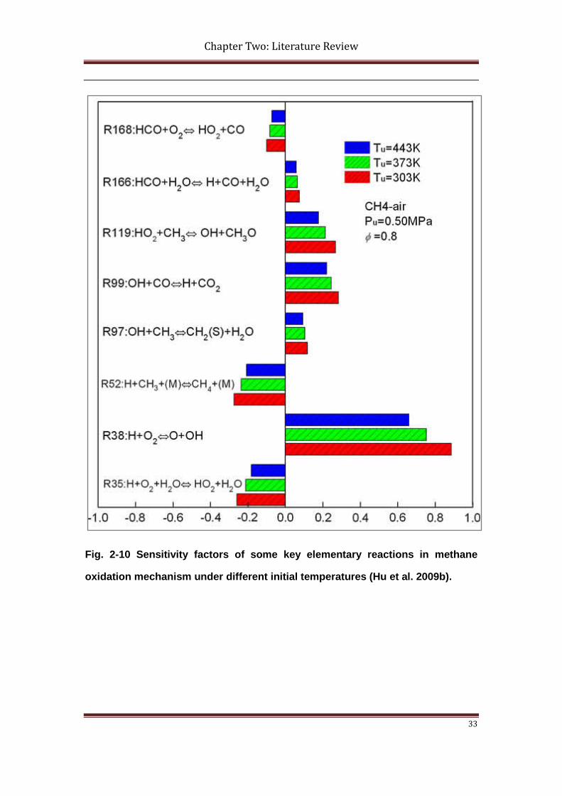
Chapter Two: Literature Review
33
Fig. 2-10 Sensitivity factors of some key elementary reactions in methane
oxidation mechanism under different initial temperatures (Hu et al. 2009b).
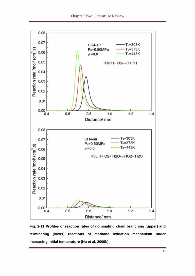
Chapter Two: Literature Review
34
Fig. 2-11 Profiles of reaction rates of dominating chain branching (upper) and
terminating (lower) reactions of methane oxidation mechanism under
increasing initial temperature (Hu et al. 2009b).
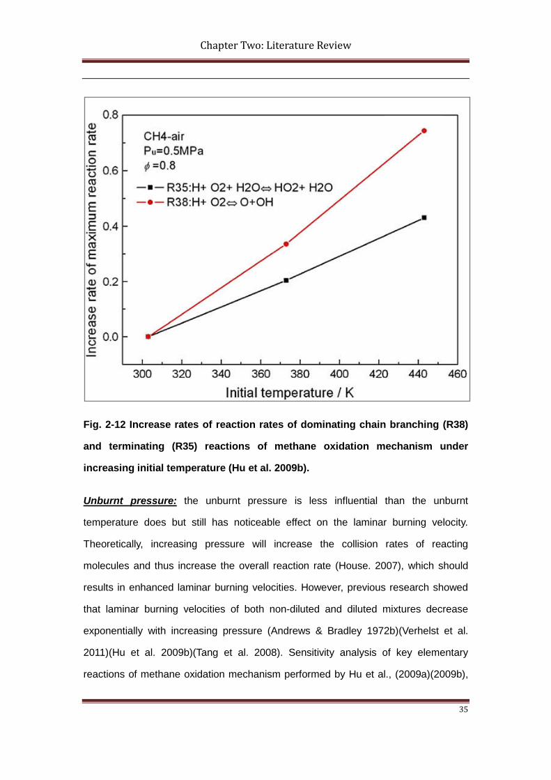
Chapter Two: Literature Review
35
Fig. 2-12 Increase rates of reaction rates of dominating chain branching (R38)
and terminating (R35) reactions of methane oxidation mechanism under
increasing initial temperature (Hu et al. 2009b).
Unburnt pressure: the unburnt pressure is less influential than the unburnt
temperature does but still has noticeable effect on the laminar burning velocity.
Theoretically, increasing pressure will increase the collision rates of reacting
molecules and thus increase the overall reaction rate (House. 2007), which should
results in enhanced laminar burning velocities. However, previous research showed
that laminar burning velocities of both non-diluted and diluted mixtures decrease
exponentially with increasing pressure (Andrews & Bradley 1972b)(Verhelst et al.
2011)(Hu et al. 2009b)(Tang et al. 2008). Sensitivity analysis of key elementary
reactions of methane oxidation mechanism performed by Hu et al., (2009a)(2009b),
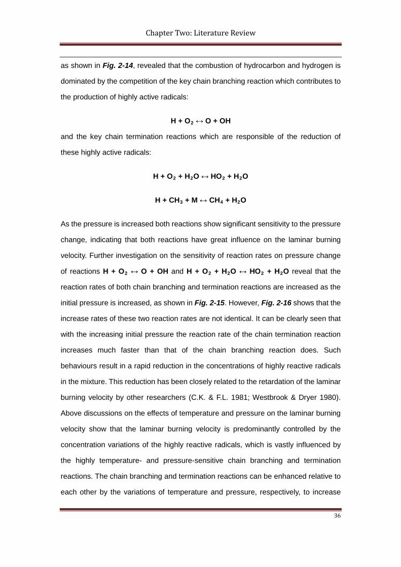
Chapter Two: Literature Review
36
as shown in Fig. 2-14, revealed that the combustion of hydrocarbon and hydrogen is
dominated by the competition of the key chain branching reaction which contributes to
the production of highly active radicals:
H + O2 ↔ O + OH
and the key chain termination reactions which are responsible of the reduction of
these highly active radicals:
H + O2 + H2O ↔ HO2 + H2O
H + CH3 + M ↔ CH4 + H2O
As the pressure is increased both reactions show significant sensitivity to the pressure
change, indicating that both reactions have great influence on the laminar burning
velocity. Further investigation on the sensitivity of reaction rates on pressure change
of reactions H + O2 ↔ O + OH and H + O2 + H2O ↔ HO2 + H2O reveal that the
reaction rates of both chain branching and termination reactions are increased as the
initial pressure is increased, as shown in Fig. 2-15. However, Fig. 2-16 shows that the
increase rates of these two reaction rates are not identical. It can be clearly seen that
with the increasing initial pressure the reaction rate of the chain termination reaction
increases much faster than that of the chain branching reaction does. Such
behaviours result in a rapid reduction in the concentrations of highly reactive radicals
in the mixture. This reduction has been closely related to the retardation of the laminar
burning velocity by other researchers (C.K. & F.L. 1981; Westbrook & Dryer 1980).
Above discussions on the effects of temperature and pressure on the laminar burning
velocity show that the laminar burning velocity is predominantly controlled by the
concentration variations of the highly reactive radicals, which is vastly influenced by
the highly temperature- and pressure-sensitive chain branching and termination
reactions. The chain branching and termination reactions can be enhanced relative to
each other by the variations of temperature and pressure, respectively, to increase
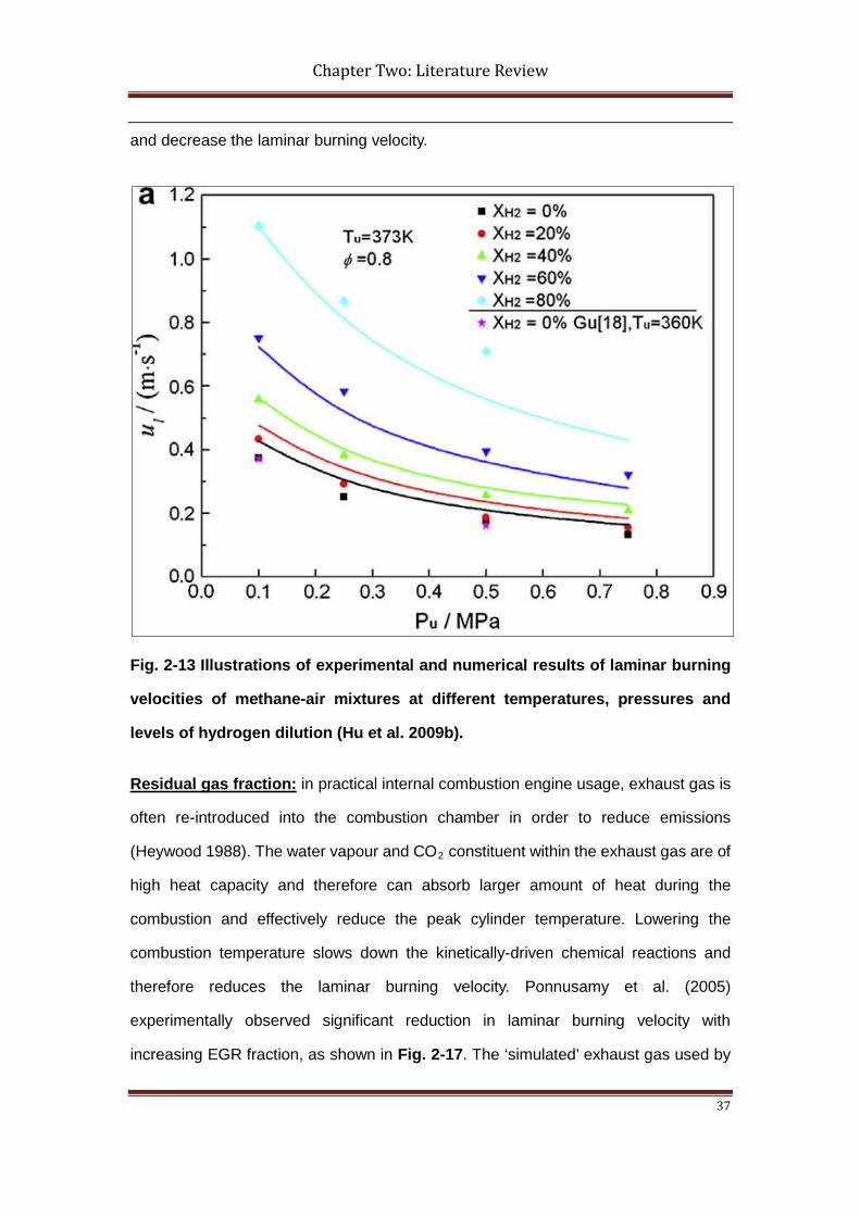
Chapter Two: Literature Review
37
and decrease the laminar burning velocity.
Fig. 2-13 Illustrations of experimental and numerical results of laminar burning
velocities of methane-air mixtures at different temperatures, pressures and
levels of hydrogen dilution (Hu et al. 2009b).
Residual gas fraction: in practical internal combustion engine usage, exhaust gas is
often re-introduced into the combustion chamber in order to reduce emissions
(Heywood 1988). The water vapour and CO2 constituent within the exhaust gas are of
high heat capacity and therefore can absorb larger amount of heat during the
combustion and effectively reduce the peak cylinder temperature. Lowering the
combustion temperature slows down the kinetically-driven chemical reactions and
therefore reduces the laminar burning velocity. Ponnusamy et al. (2005)
experimentally observed significant reduction in laminar burning velocity with
increasing EGR fraction, as shown in Fig. 2-17. The ‘simulated’ exhaust gas used by
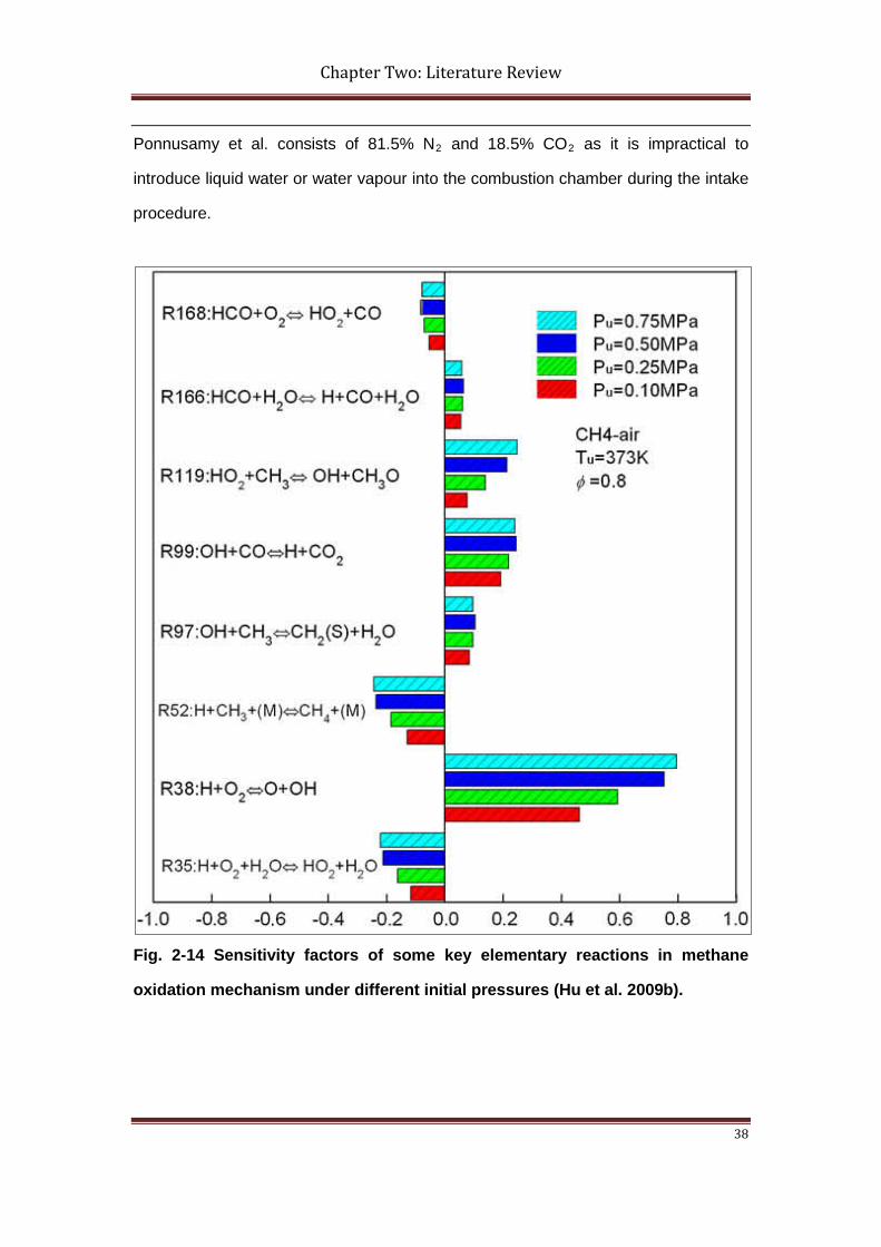
Chapter Two: Literature Review
38
Ponnusamy et al. consists of 81.5% N2 and 18.5% CO2 as it is impractical to
introduce liquid water or water vapour into the combustion chamber during the intake
procedure.
Fig. 2-14 Sensitivity factors of some key elementary reactions in methane
oxidation mechanism under different initial pressures (Hu et al. 2009b).
Chapter Two: Literature Review
39
Fig. 2-15 Profiles of reaction rates of dominating chain branching (upper) and
terminating (lower) reactions of methane oxidation mechanism under
increasing initial pressure (Hu et al. 2009b).
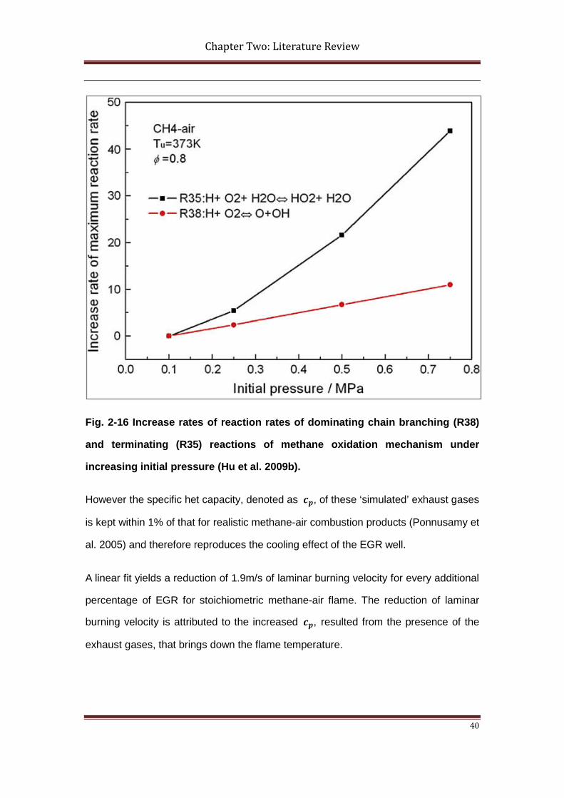
Chapter Two: Literature Review
40
Fig. 2-16 Increase rates of reaction rates of dominating chain branching (R38)
and terminating (R35) reactions of methane oxidation mechanism under
increasing initial pressure (Hu et al. 2009b).
However the specific het capacity, denoted as 𝒄𝒑, of these ‘simulated’ exhaust gases
is kept within 1% of that for realistic methane-air combustion products (Ponnusamy et
al. 2005) and therefore reproduces the cooling effect of the EGR well.
A linear fit yields a reduction of 1.9m/s of laminar burning velocity for every additional
percentage of EGR for stoichiometric methane-air flame. The reduction of laminar
burning velocity is attributed to the increased 𝒄𝒑, resulted from the presence of the
exhaust gases, that brings down the flame temperature.
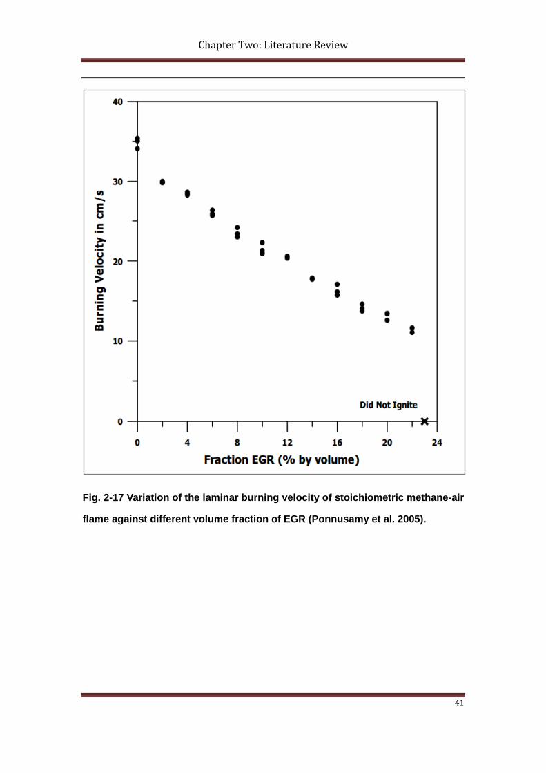
Chapter Two: Literature Review
41
Fig. 2-17 Variation of the laminar burning velocity of stoichiometric methane-air
flame against different volume fraction of EGR (Ponnusamy et al. 2005).
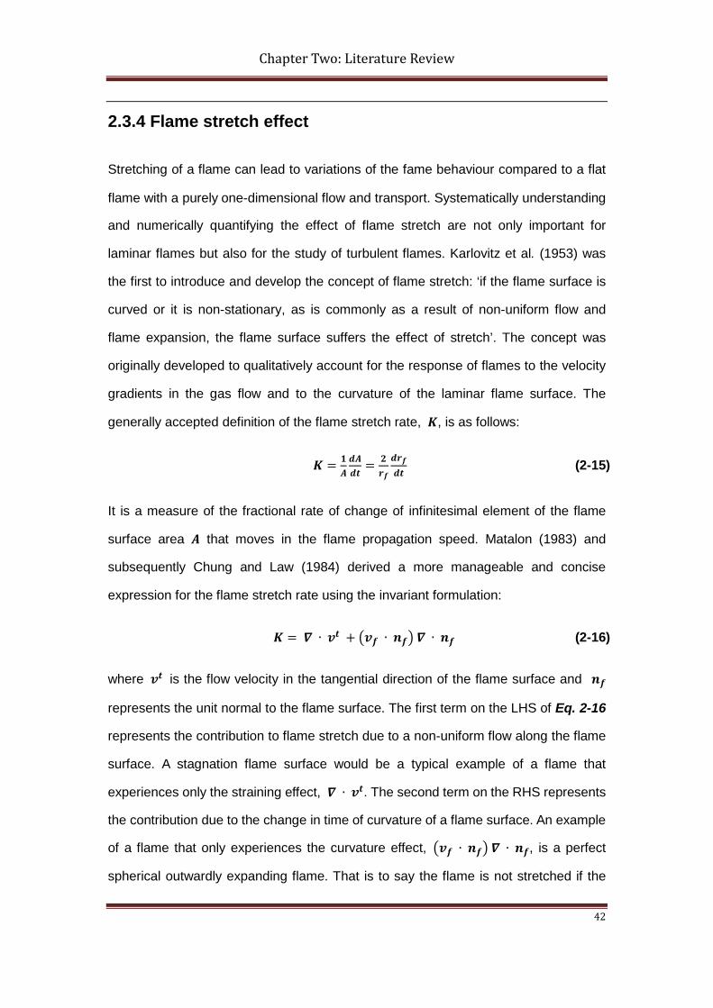
Chapter Two: Literature Review
42
2.3.4 Flame stretch effect
Stretching of a flame can lead to variations of the fame behaviour compared to a flat
flame with a purely one-dimensional flow and transport. Systematically understanding
and numerically quantifying the effect of flame stretch are not only important for
laminar flames but also for the study of turbulent flames. Karlovitz et al. (1953) was
the first to introduce and develop the concept of flame stretch: ‘if the flame surface is
curved or it is non-stationary, as is commonly as a result of non-uniform flow and
flame expansion, the flame surface suffers the effect of stretch’. The concept was
originally developed to qualitatively account for the response of flames to the velocity
gradients in the gas flow and to the curvature of the laminar flame surface. The
generally accepted definition of the flame stretch rate, 𝑲, is as follows:
𝑲 = 𝟏𝑨𝒂𝑨𝒂𝒕
= 𝟐𝑷𝒇
𝒂𝑷𝒇𝒂𝒕
(2-15)
It is a measure of the fractional rate of change of infinitesimal element of the flame
surface area 𝑨 that moves in the flame propagation speed. Matalon (1983) and
subsequently Chung and Law (1984) derived a more manageable and concise
expression for the flame stretch rate using the invariant formulation:
𝑲 = 𝜵 ∙ 𝒗𝒕 + �𝒗𝒇 ∙ 𝒏𝒇� 𝜵 ∙ 𝒏𝒇 (2-16)
where 𝒗𝒕 is the flow velocity in the tangential direction of the flame surface and 𝒏𝒇
represents the unit normal to the flame surface. The first term on the LHS of Eq. 2-16
represents the contribution to flame stretch due to a non-uniform flow along the flame
surface. A stagnation flame surface would be a typical example of a flame that
experiences only the straining effect, 𝜵 ∙ 𝒗𝒕. The second term on the RHS represents
the contribution due to the change in time of curvature of a flame surface. An example
of a flame that only experiences the curvature effect, �𝒗𝒇 ∙ 𝒏𝒇� 𝜵 ∙ 𝒏𝒇, is a perfect
spherical outwardly expanding flame. That is to say the flame is not stretched if the
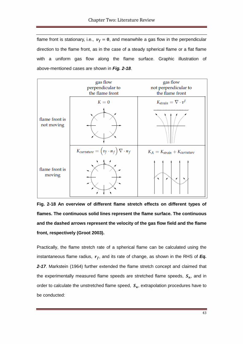
Chapter Two: Literature Review
43
flame front is stationary, i.e., 𝒗𝒇 = 𝟏, and meanwhile a gas flow in the perpendicular
direction to the flame front, as in the case of a steady spherical flame or a flat flame
with a uniform gas flow along the flame surface. Graphic illustration of
above-mentioned cases are shown in Fig. 2-18.
Fig. 2-18 An overview of different flame stretch effects on different types of
flames. The continuous solid lines represent the flame surface. The continuous
and the dashed arrows represent the velocity of the gas flow field and the flame
front, respectively (Groot 2003).
Practically, the flame stretch rate of a spherical flame can be calculated using the
instantaneous flame radius, 𝑷𝒇, and its rate of change, as shown in the RHS of Eq.
2-17. Markstein (1964) further extended the flame stretch concept and claimed that
the experimentally measured flame speeds are stretched flame speeds, 𝑺𝒏, and in
order to calculate the unstretched flame speed, 𝑺𝒖, extrapolation procedures have to
be conducted:
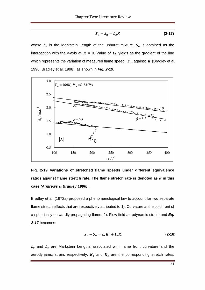
Chapter Two: Literature Review
44
𝑺𝒖 − 𝑺𝒏 = 𝑳𝒃𝑲 (2-17)
where 𝑳𝒃 is the Markstein Length of the unburnt mixture. 𝑺𝒖 R is obtained as the
interception with the y-axis at 𝑲 = 0. Value of 𝑳𝒃 yields as the gradient of the line
which represents the variation of measured flame speed, 𝑺𝒏, against 𝑲P
(Bradley et al.
1996; Bradley et al. 1998), as shown in Fig. 2-19.
Fig. 2-19 Variations of stretched flame speeds under different equivalence
ratios against flame stretch rate. The flame stretch rate is denoted as α in this
case (Andrews & Bradley 1996) .
Bradley et al. (1972a) proposed a phenomenological law to account for two separate
flame stretch effects that are respectively attributed to 1). Curvature at the cold front of
a spherically outwardly propagating flame, 2). Flow field aerodynamic strain, and Eq.
2-17 becomes:
𝑺𝒖 − 𝑺𝒏 = 𝑳𝒄𝑲𝒄 + 𝑳𝒅𝑲𝒅 (2-18)
𝑳𝒄 and 𝑳𝒄 are Markstein Lengths associated with flame front curvature and the
aerodynamic strain, respectively. 𝑲𝒄 and 𝑲𝒅 are the corresponding stretch rates.
Chapter Two: Literature Review
45
Detailed methodology of deriving 𝑺𝒖, 𝑳𝒄 and 𝑳𝒅 are stated by Bradley et al. (1972a).
The two separate Markstein Lengths are usually combined into one single Markstein
Length in practice, as proposed by Bechtold et al. (2001):
𝑳 = 𝜹[𝜶 − (𝝈 − 𝟏)𝜸𝟏/𝝈] (2-19)
For the sake of convenience, the Markstein Length is often normalised by the flame
thickness, 𝜹𝒇, to give a dimensionless parameter Markstein Number, 𝑴𝑫:
𝑴𝑫 = 𝑳/𝜹𝒇 (2-20)
The Markstein Number is very sensitive to fuel type, mixture strength and system
pressure. Bechtold et al. (2001) measured the Markstein Number for different types of
fuels at different equivalence ratios, as shown in Fig. 2-20. The number of carbon
contents in the fuel molecules have a dominant effect on Markstein Number. Fuels
with higher carbon contents have higher Markstein Number and the Markstein
Number decreases with increasing equivalence ratio, in a manner such that the higher
the carbon contents the faster the Markstein Number decreases. However, simple
hydrocarbon fuels such as Methane with only one carbon atom and non-hydrocarbon
fuels such as Hydrogen show the opposite behaviour. Lean hydrogen-air mixtures
also show negative Markstein Number which indicates the existence of negative
flame stretch that is not found in hydrocarbon fuels.
The Markstein Number is also found to decrease with increasing pressure for
stoichiometric and lean iso-octane/ air mixture (Bechtold & Matalon 2001). This
phenomenon indicates a decreasing influence of the flame stretch on the laminar
burning velocity at higher pressures. Increasing the temperature can partially restore
the effectiveness of the flame stretch only at pressures higher than 2.5bar, and would
otherwise worsen the effect of the flame stretch.

Chapter Two: Literature Review
46
Fig. 2-20 Markstein Number of different types of fuel-air mixtures under
different equivalence ratios (Bechtold & Matalon 2001).
Markstein Number has also been proven to have important influence on flame
instabilities (Kwon & Faeth 2001). Although in S.I. engines the spark ignited flame will
eventually become unstable and flame instabilities can enhance the burn rate, early
destabilization is not favoured. Flames have higher Markstein Number, i.e., higher
flame stretch rate, in the early stages of their growth and therefore it helps to stabilise
the flames against hydrodynamic instabilities through the flame-stretch-induced
thermo-diffusive effects. The larger the Markstein Number the greater the stabilization
effect. As the flame grows the flame stretch decreases because of the reduction in
surface curvature, so as the stabilization effect. Therefore the flame is more
vulnerable to surface cellularity which eventually leads to self-turbulising. Early
self-turbulising of flame can result in total distortion of flame surface and flame
Chapter Two: Literature Review
47
extinction and thus should be avoided. Negative Markstein Number is also found to be
responsible for preferential-diffusion instability (Kwon & Faeth 2001).
Lewis Number is another key parameter in the studies of flame stretch. In one-step
reaction mechanisms with large activation energies, Lewis Number is the differential
diffusion of heat and deficient reactant (Kwon & Faeth 2001):
𝑳𝑹 = 𝝀𝝆𝑪𝒑𝑫
(2-21)
where the term 𝝀/𝝆𝑪𝒑 represents the thermal diffusivity of the mixture and the term D
is the mass diffusivity of the deficient reactant. It has been long proven that cellular
flames tend to form in mixtures that are deficient in the light reactants, such as in rich
heavy hydrocarbon-air mixtures (n-heptane, iso-octane, etc) and lean light
hydrocarbon-air mixtures (methane, hydrogen etc). The formation of cellular surface
is partially due to thermo-diffusive instabilities, which is originally caused by
competing effects of heat conduction from, and reactant diffusion into, the flame front.
Smooth flame surface can be unstable when the mass diffusivity of the deficient
reactant is greater than the heat diffusivity of the mixture, i.e., when 𝑳𝑹 < 1 (Bechtold
& Matalon 1987). Flames suffers thermo-diffusive instability can be unstable from the
initial stage of propagation. Some researchers (Peters 2000) concluded that cellular
patterns will form for 𝑳𝑹 < 1 because the initial perturbation of the flame front is
enhanced, while the 𝑳𝑹 > 1 case is stabilizing. However in some research works
(Groff 1982)(Simon & Wong 1953), instable flame surfaces are observed for mixtures
with 𝑳𝑹 > 1. Bechtold et al. (1987) conclude that this is a result of the hydrodynamic
instability, which arise from thermal expansion generated by interaction between
flame and the hydrodynamic disturbances. Various experimental observations
showed that hydrodynamic instability occurs only when the flame reaches a critical
value. Bechtold et al. (1987) proposed a critical value for Lewis Number:
𝑳𝑹∗ = 𝟏 − 𝝈𝟐𝑸𝟏𝑸𝟐𝑬
(2-22)
Chapter Two: Literature Review
48
where 𝑸𝟏 and 𝑸𝟐 are empirical coefficients, derived in (Aung et al. 1997). It is also
found that in most cases the critical Lewis Number is less than unity, which indicates
that the rate of heat loss from the flame front has to be, by some margin, less than the
rate of deficient mass flow into the flame front in order to maintain a stable flame.
Influences of chemistry and heat loss have been widely analysed. Under the
assumption of one-step chemistry mechanism with large activation energy, non-unity
Lewis Number induces a temperature change in the thin reaction layer, to which the
burning velocity is very sensitive (Libby & Williams 1982; Libby & Williams 1983).
Lewis Number larger than one causes excessive heat losses and promotes flame
extinction, which can be retarded by density effect. By applying two-step reaction
mechanism, Tam et al. (1984) found that, asymptotically, in weak flame stretch
conditions reaction intermediate products are effective in retarding flame extinction, if
the activation energy of the first reaction is large. Other researchers concluded as well
that these intermediates influence the flame’s response to stretch (Peters & Smooke
1985).
In situations where the Lewis Number deviates significantly from unity, its effect is
amplified. Peters et al. (1985) tested stretched lean (Φ=0.6) and rich (Φ=1.4)
hydrogen-air flames with elementary kinetics. Due to the large diffusivity of hydrogen
the Lewis Number is 0.31 for the lean mixture and due to large thermal diffusivity it is
3.02 in the rich case. The results show that in both cases, the effect of Lewis Number
is dominating over the details of chemical kinetics. Extinction is observed for positive
stretch in rich Hydrogen flames (𝑳𝑹 > 𝟏).
2.4 Turbulent flames
When a laminar flame is entering a turbulent flow field the combustion regime of the
flame is then replaced by one where the turbulence and the flame interact. Turbulent
combustion results from the two-way interaction of chemistry and turbulence. When a
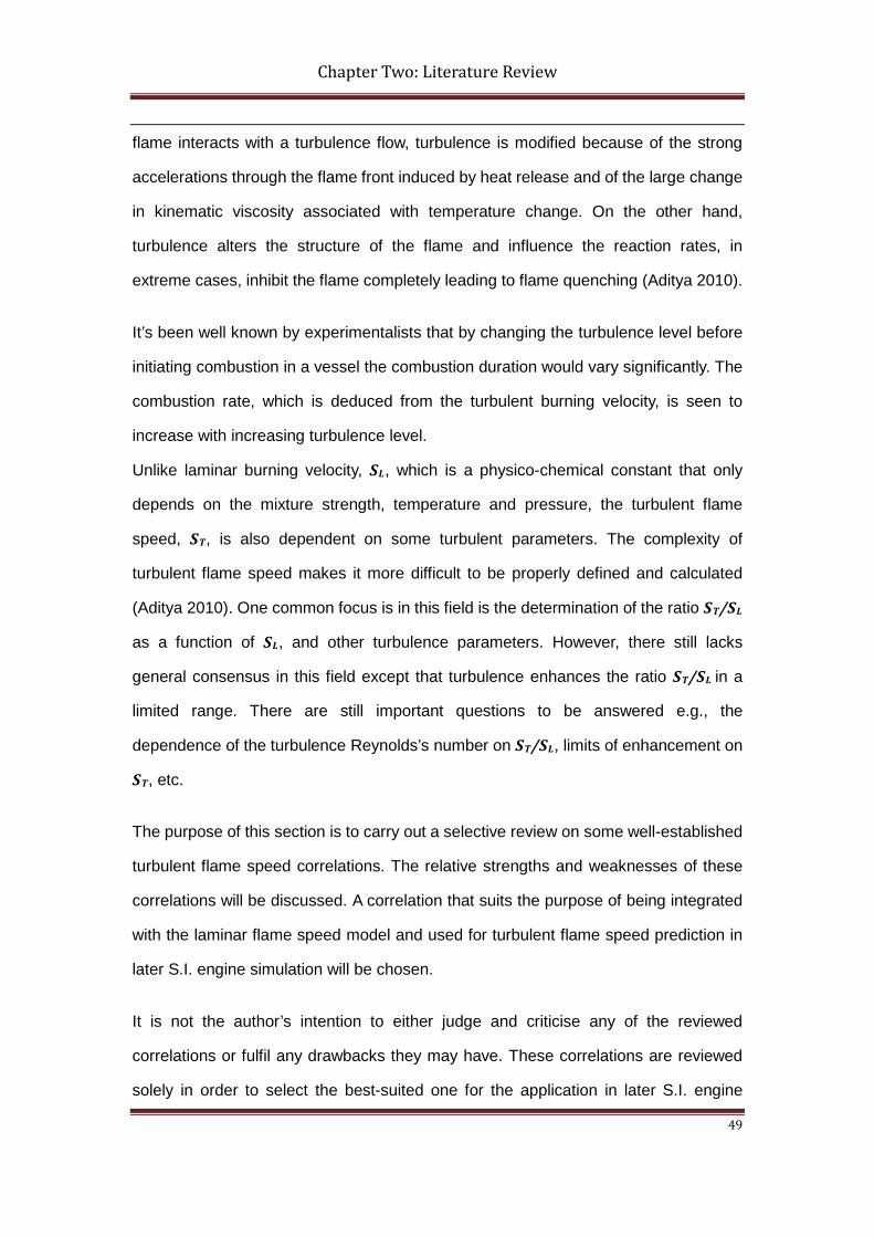
Chapter Two: Literature Review
49
flame interacts with a turbulence flow, turbulence is modified because of the strong
accelerations through the flame front induced by heat release and of the large change
in kinematic viscosity associated with temperature change. On the other hand,
turbulence alters the structure of the flame and influence the reaction rates, in
extreme cases, inhibit the flame completely leading to flame quenching (Aditya 2010).
It’s been well known by experimentalists that by changing the turbulence level before
initiating combustion in a vessel the combustion duration would vary significantly. The
combustion rate, which is deduced from the turbulent burning velocity, is seen to
increase with increasing turbulence level.
Unlike laminar burning velocity, SL, which is a physico-chemical constant that only
depends on the mixture strength, temperature and pressure, the turbulent flame
speed, ST, is also dependent on some turbulent parameters. The complexity of
turbulent flame speed makes it more difficult to be properly defined and calculated
(Aditya 2010). One common focus is in this field is the determination of the ratio ST/SL
as a function of SL, and other turbulence parameters. However, there still lacks
general consensus in this field except that turbulence enhances the ratio ST/SL in a
limited range. There are still important questions to be answered e.g., the
dependence of the turbulence Reynolds’s number on ST/SL, limits of enhancement on
ST, etc.
The purpose of this section is to carry out a selective review on some well-established
turbulent flame speed correlations. The relative strengths and weaknesses of these
correlations will be discussed. A correlation that suits the purpose of being integrated
with the laminar flame speed model and used for turbulent flame speed prediction in
later S.I. engine simulation will be chosen.
It is not the author’s intention to either judge and criticise any of the reviewed
correlations or fulfil any drawbacks they may have. These correlations are reviewed
solely in order to select the best-suited one for the application in later S.I. engine
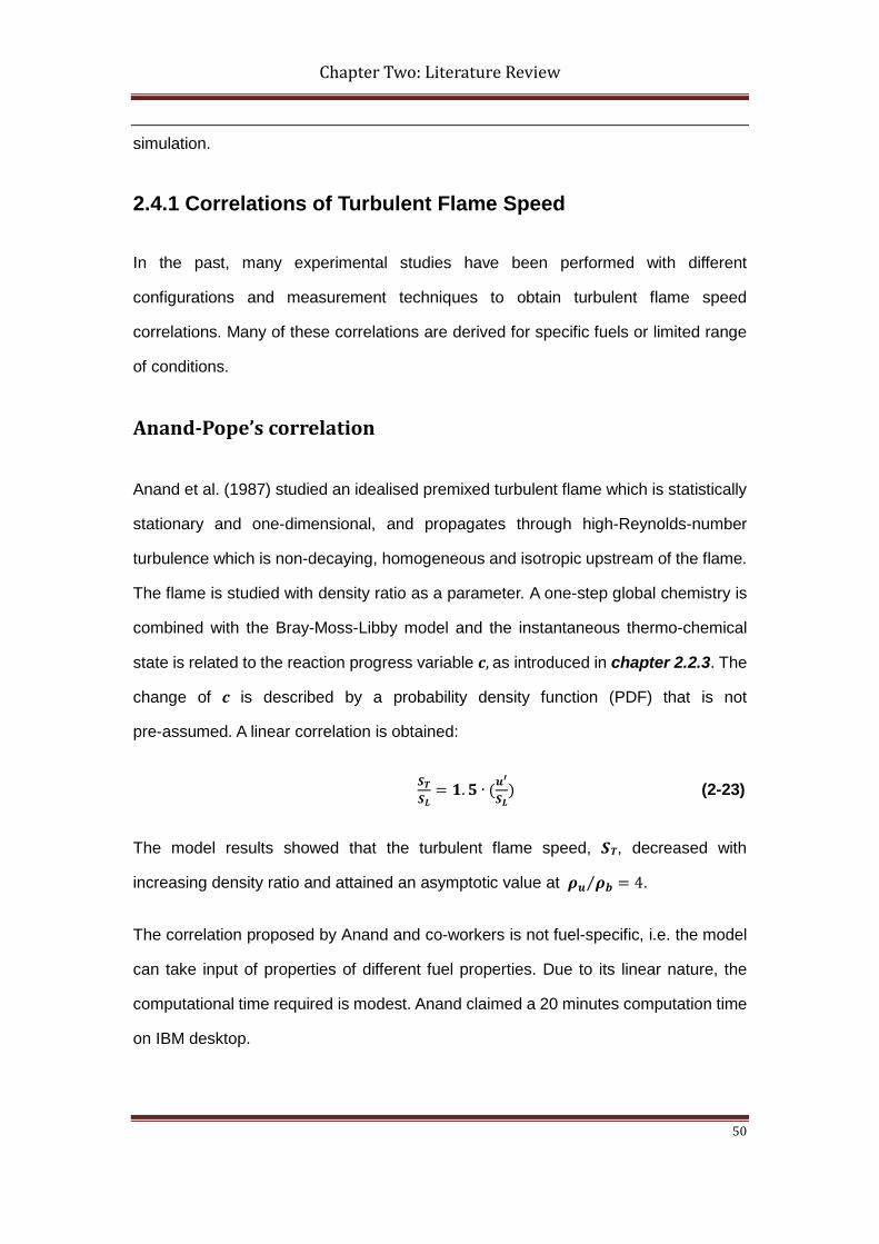
Chapter Two: Literature Review
50
simulation.
2.4.1 Correlations of Turbulent Flame Speed
In the past, many experimental studies have been performed with different
configurations and measurement techniques to obtain turbulent flame speed
correlations. Many of these correlations are derived for specific fuels or limited range
of conditions.
Anand-Pope’s correlation
Anand et al. (1987) studied an idealised premixed turbulent flame which is statistically
stationary and one-dimensional, and propagates through high-Reynolds-number
turbulence which is non-decaying, homogeneous and isotropic upstream of the flame.
The flame is studied with density ratio as a parameter. A one-step global chemistry is
combined with the Bray-Moss-Libby model and the instantaneous thermo-chemical
state is related to the reaction progress variable c, as introduced in chapter 2.2.3. The
change of c is described by a probability density function (PDF) that is not
pre-assumed. A linear correlation is obtained:
𝑺𝑻𝑺𝑳
= 𝟏.𝟓 ∙ (𝒖′
𝑺𝑳) (2-23)
The model results showed that the turbulent flame speed, ST, decreased with
increasing density ratio and attained an asymptotic value at 𝝆𝒖 𝝆𝒃⁄ = 4.
The correlation proposed by Anand and co-workers is not fuel-specific, i.e. the model
can take input of properties of different fuel properties. Due to its linear nature, the
computational time required is modest. Anand claimed a 20 minutes computation time
on IBM desktop.
Chapter Two: Literature Review
51
Fig. 2-21 Normalised turbulent flame speed against density ratio (Anand & Pope
1987).
Wirth-Peters’ correlation
Wirth and Peters (1992) measured turbulent flame speeds for propane-air flames
using a VW transparent engine. The engine is a four-cylinder, 1.6L unit with
bore/stroke ratio of 79.5/80mm and a compression ratio of 8.5. The optical access is
provided by via elongated crankcase and pistons with quartz window in the piston
crown of about 58mm in diameter. Three additional square windows, 20 by 20mm, are
placed into the cylinder wall beneath the cylinder head to provide three-dimensional
optical access. Experiments were carried out using laser tomographic technique with
Nd:YAG laser pulse. Experimental results revealed a decreasing trend of turbulence
structure size.
Chapter Two: Literature Review
52
Fig. 2-22 Schematic of the VW transparent engine, optical layout and imaged
area in the combustion chamber (Wirth & Peters 1992).
Wirth and Peters derived a flamelet formation for premixed turbulent flames based on
a scalar field equation that describes the instantaneous flame front location in the
turbulent flow field. The differential equation derived represents the local kinematic
balance between fluid flow velocity, burning velocity and flame propagation velocity. A
spectral closure of the problem was performed on the basis of a two-point correlation:
𝑺𝑻𝑺𝑳
= 𝟏 + 𝟏.𝟔(𝒖𝒕′
𝑺𝑳)𝟏.𝟓 + 𝟏.𝟓(𝒖𝒕
′
𝑺𝑳) (2-24)
This correlation also includes the effects of flame stretch, which is seen as the sum of
tangential strain and flame front curvature. Two key assumption made in the
derivation are that the response of flame to a train field is instantaneous and
time-varying strains only influence the flame at the mean property level. By applying
these assumption, the derived correlation is only valid for turbulence flames in which
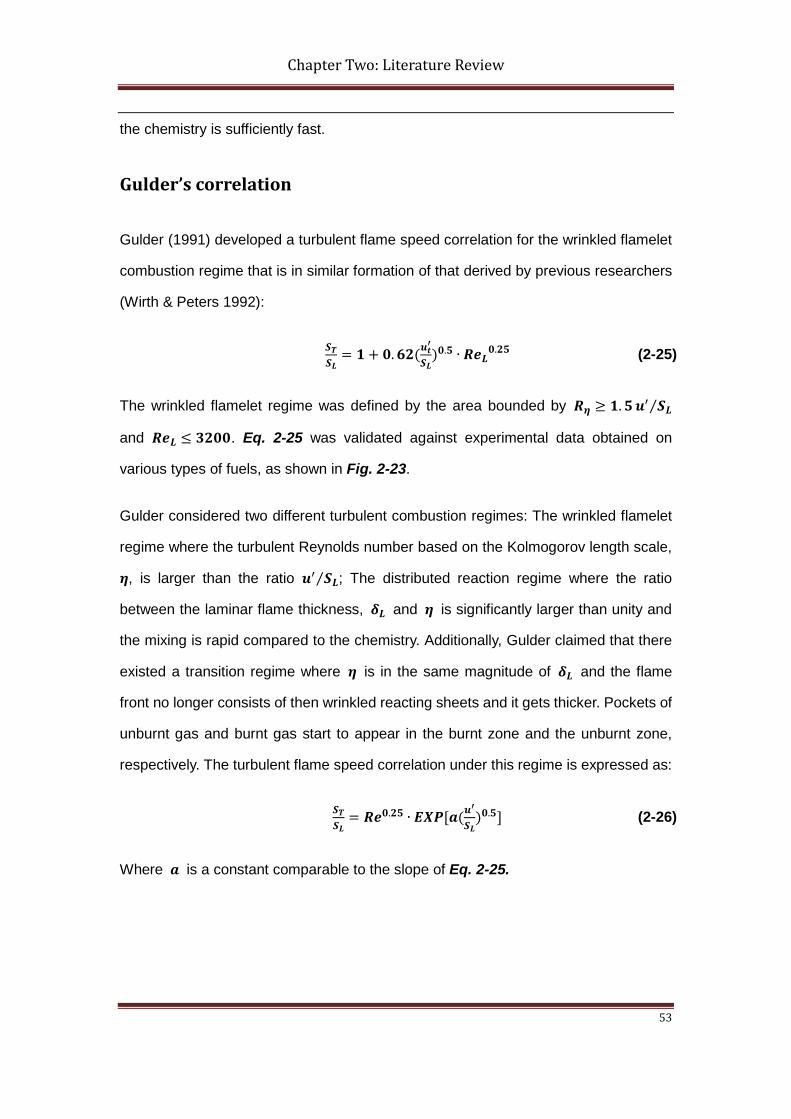
Chapter Two: Literature Review
53
the chemistry is sufficiently fast.
Gulder’s correlation
Gulder (1991) developed a turbulent flame speed correlation for the wrinkled flamelet
combustion regime that is in similar formation of that derived by previous researchers
(Wirth & Peters 1992):
𝑺𝑻𝑺𝑳
= 𝟏 + 𝟏.𝟔𝟐(𝒖𝒕′
𝑺𝑳)𝟏.𝟓 ∙ 𝑹𝑹𝑳𝟏.𝟐𝟓 (2-25)
The wrinkled flamelet regime was defined by the area bounded by 𝑹𝜼 ≥ 𝟏.𝟓𝒖′ 𝑺𝑳⁄
and 𝑹𝑹𝑳 ≤ 𝟑𝟐𝟏𝟏. Eq. 2-25 was validated against experimental data obtained on
various types of fuels, as shown in Fig. 2-23.
Gulder considered two different turbulent combustion regimes: The wrinkled flamelet
regime where the turbulent Reynolds number based on the Kolmogorov length scale,
𝜼, is larger than the ratio 𝒖′ 𝑺𝑳⁄ ; The distributed reaction regime where the ratio
between the laminar flame thickness, 𝜹𝑳 and 𝜼 is significantly larger than unity and
the mixing is rapid compared to the chemistry. Additionally, Gulder claimed that there
existed a transition regime where 𝜼 is in the same magnitude of 𝜹𝑳 and the flame
front no longer consists of then wrinkled reacting sheets and it gets thicker. Pockets of
unburnt gas and burnt gas start to appear in the burnt zone and the unburnt zone,
respectively. The turbulent flame speed correlation under this regime is expressed as:
𝑺𝑻𝑺𝑳
= 𝑹𝑹𝟏.𝟐𝟓 ∙ 𝑬𝑬𝑷[𝑫(𝒖′
𝑺𝑳)𝟏.𝟓] (2-26)
Where 𝑫 is a constant comparable to the slope of Eq. 2-25.
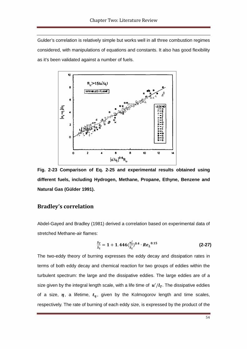
Chapter Two: Literature Review
54
Gulder’s correlation is relatively simple but works well in all three combustion regimes
considered, with manipulations of equations and constants. It also has good flexibility
as it’s been validated against a number of fuels.
Fig. 2-23 Comparison of Eq. 2-25 and experimental results obtained using
different fuels, including Hydrogen, Methane, Propane, Ethyne, Benzene and
Natural Gas (Gülder 1991).
Bradley’s correlation
Abdel-Gayed and Bradley (1981) derived a correlation based on experimental data of
stretched Methane-air flames:
𝑺𝑻𝑺𝑳
= 𝟏 + 𝟏.𝟒𝟒𝟔(𝒖𝒕′
𝑺𝑳)𝟏.𝟒 ∙ 𝑹𝑹𝑳𝟏.𝟏𝟓 (2-27)
The two-eddy theory of burning expresses the eddy decay and dissipation rates in
terms of both eddy decay and chemical reaction for two groups of eddies within the
turbulent spectrum: the large and the dissipative eddies. The large eddies are of a
size given by the integral length scale, with a life time of 𝒖′/𝒍𝑻. The dissipative eddies
of a size, 𝜼 , a lifetime, 𝒕𝜼 , given by the Kolmogorov length and time scales,
respectively. The rate of burning of each eddy size, is expressed by the product of the
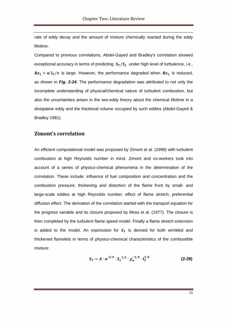
Chapter Two: Literature Review
55
rate of eddy decay and the amount of mixture chemically reacted during the eddy
lifetime.
Compared to previous correlations, Abdel-Gayed and Bradley’s correlation showed
exceptional accuracy in terms of predicting 𝑺𝑻 𝑺𝑳⁄ under high level of turbulence, i.e.,
𝑹𝑹𝑳 = 𝒖′𝒍𝑻 𝝂⁄ is large. However, the performance degraded when 𝑹𝑹𝑳 is reduced,
as shown in Fig. 2-24. The performance degradation was attributed to not only the
incomplete understanding of physical/chemical nature of turbulent combustion, but
also the uncertainties arisen in the two-eddy theory about the chemical lifetime in a
dissipative eddy and the fractional volume occupied by such eddies (Abdel-Gayed &
Bradley 1981).
Zimont’s correlation
An efficient computational model was proposed by Zimont et al. (1998) with turbulent
combustion at high Reynolds number in mind. Zimont and co-workers took into
account of a series of physico-chemical phenomena in the determination of the
correlation. These include: influence of fuel composition and concentration and the
combustion pressure; thickening and distortion of the flame front by small- and
large-scale eddies at high Reynolds number; effect of flame stretch; preferential
diffusion effect. The derivation of the correlation started with the transport equation for
the progress variable and its closure proposed by Moss et al. (1977). The closure is
then completed by the turbulent flame speed model. Finally a flame stretch extension
is added to the model. An expression for 𝑺𝑻 is derived for both wrinkled and
thickened flamelets in terms of physico-chemical characteristics of the combustible
mixture:
𝑺𝑻 = 𝑨 ∙ 𝒖′𝟑/𝟒 ∙ 𝑺𝑳𝟏/𝟐 ∙ 𝝌𝒖−𝟏/𝟒 ∙ 𝒍𝑻
𝟏/𝟒 (2-28)
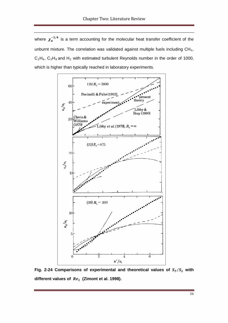
Chapter Two: Literature Review
56
where 𝝌𝒖−𝟏/𝟒 is a term accounting for the molecular heat transfer coefficient of the
unburnt mixture. The correlation was validated against multiple fuels including CH4,
C2H6, C3H8 and H2 with estimated turbulent Reynolds number in the order of 1000,
which is higher than typically reached in laboratory experiments.
Fig. 2-24 Comparisons of experimental and theoretical values of 𝑺𝑻 𝑺𝑳⁄ with
different values of 𝑹𝑹𝑳 (Zimont et al. 1998).
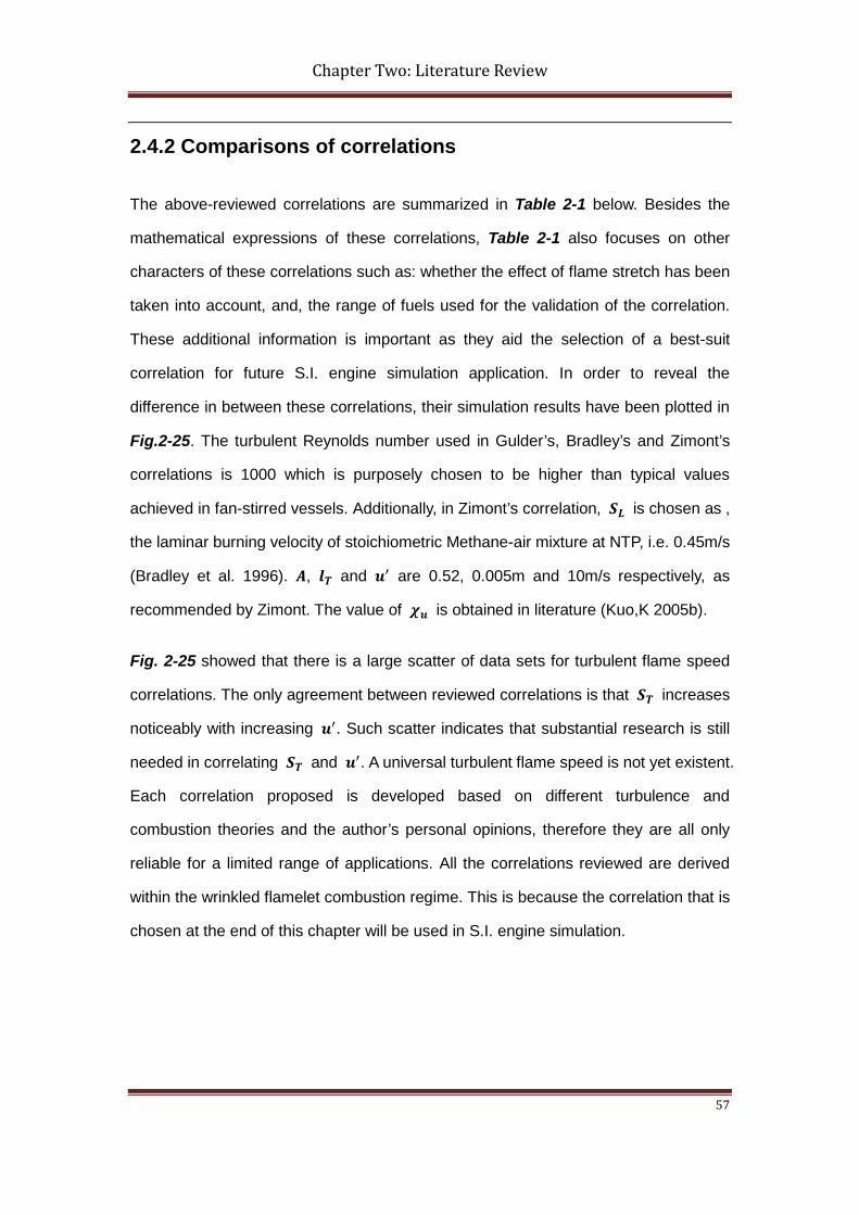
Chapter Two: Literature Review
57
2.4.2 Comparisons of correlations
The above-reviewed correlations are summarized in Table 2-1 below. Besides the
mathematical expressions of these correlations, Table 2-1 also focuses on other
characters of these correlations such as: whether the effect of flame stretch has been
taken into account, and, the range of fuels used for the validation of the correlation.
These additional information is important as they aid the selection of a best-suit
correlation for future S.I. engine simulation application. In order to reveal the
difference in between these correlations, their simulation results have been plotted in
Fig.2-25. The turbulent Reynolds number used in Gulder’s, Bradley’s and Zimont’s
correlations is 1000 which is purposely chosen to be higher than typical values
achieved in fan-stirred vessels. Additionally, in Zimont’s correlation, 𝑺𝑳 is chosen as ,
the laminar burning velocity of stoichiometric Methane-air mixture at NTP, i.e. 0.45m/s
(Bradley et al. 1996). 𝑨, 𝒍𝑻 and 𝒖′ are 0.52, 0.005m and 10m/s respectively, as
recommended by Zimont. The value of 𝝌𝒖 is obtained in literature (Kuo,K 2005b).
Fig. 2-25 showed that there is a large scatter of data sets for turbulent flame speed
correlations. The only agreement between reviewed correlations is that 𝑺𝑻 increases
noticeably with increasing 𝒖′. Such scatter indicates that substantial research is still
needed in correlating 𝑺𝑻 and 𝒖′. A universal turbulent flame speed is not yet existent.
Each correlation proposed is developed based on different turbulence and
combustion theories and the author’s personal opinions, therefore they are all only
reliable for a limited range of applications. All the correlations reviewed are derived
within the wrinkled flamelet combustion regime. This is because the correlation that is
chosen at the end of this chapter will be used in S.I. engine simulation.
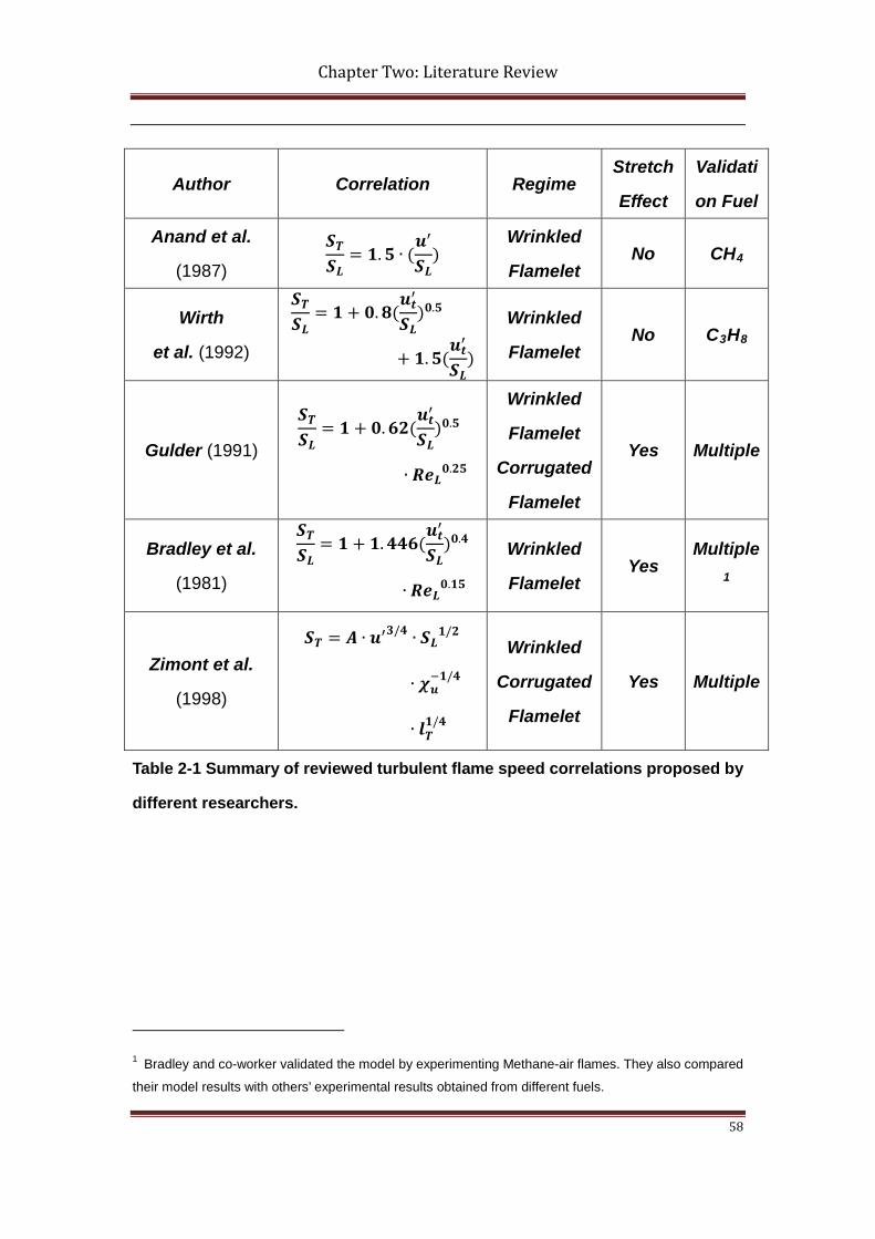
Chapter Two: Literature Review
58
Author Correlation Regime Stretch
Effect
Validati
on Fuel
Anand et al.
(1987) 𝑺𝑻𝑺𝑳
= 𝟏.𝟓 ∙ (𝒖′
𝑺𝑳)
Wrinkled
Flamelet No CH4
Wirth
et al. (1992)
𝑺𝑻𝑺𝑳
= 𝟏 + 𝟏.𝟔(𝒖𝒕′
𝑺𝑳)𝟏.𝟓
+ 𝟏.𝟓(𝒖𝒕′
𝑺𝑳)
Wrinkled
Flamelet No C3H8
Gulder (1991)
𝑺𝑻𝑺𝑳
= 𝟏 + 𝟏.𝟔𝟐(𝒖𝒕′
𝑺𝑳)𝟏.𝟓
∙ 𝑹𝑹𝑳𝟏.𝟐𝟓
Wrinkled
Flamelet
Corrugated
Flamelet
Yes Multiple
Bradley et al.
(1981)
𝑺𝑻𝑺𝑳
= 𝟏 + 𝟏.𝟒𝟒𝟔(𝒖𝒕′
𝑺𝑳)𝟏.𝟒
∙ 𝑹𝑹𝑳𝟏.𝟏𝟓
Wrinkled
Flamelet Yes
Multiple1
Zimont et al.
(1998)
𝑺𝑻 = 𝑨 ∙ 𝒖′𝟑/𝟒 ∙ 𝑺𝑳𝟏/𝟐
∙ 𝝌𝒖−𝟏/𝟒
∙ 𝒍𝑻𝟏/𝟒
Wrinkled
Corrugated
Flamelet
Yes Multiple
Table 2-1 Summary of reviewed turbulent flame speed correlations proposed by
different researchers.
1 Bradley and co-worker validated the model by experimenting Methane-air flames. They also compared
their model results with others’ experimental results obtained from different fuels.
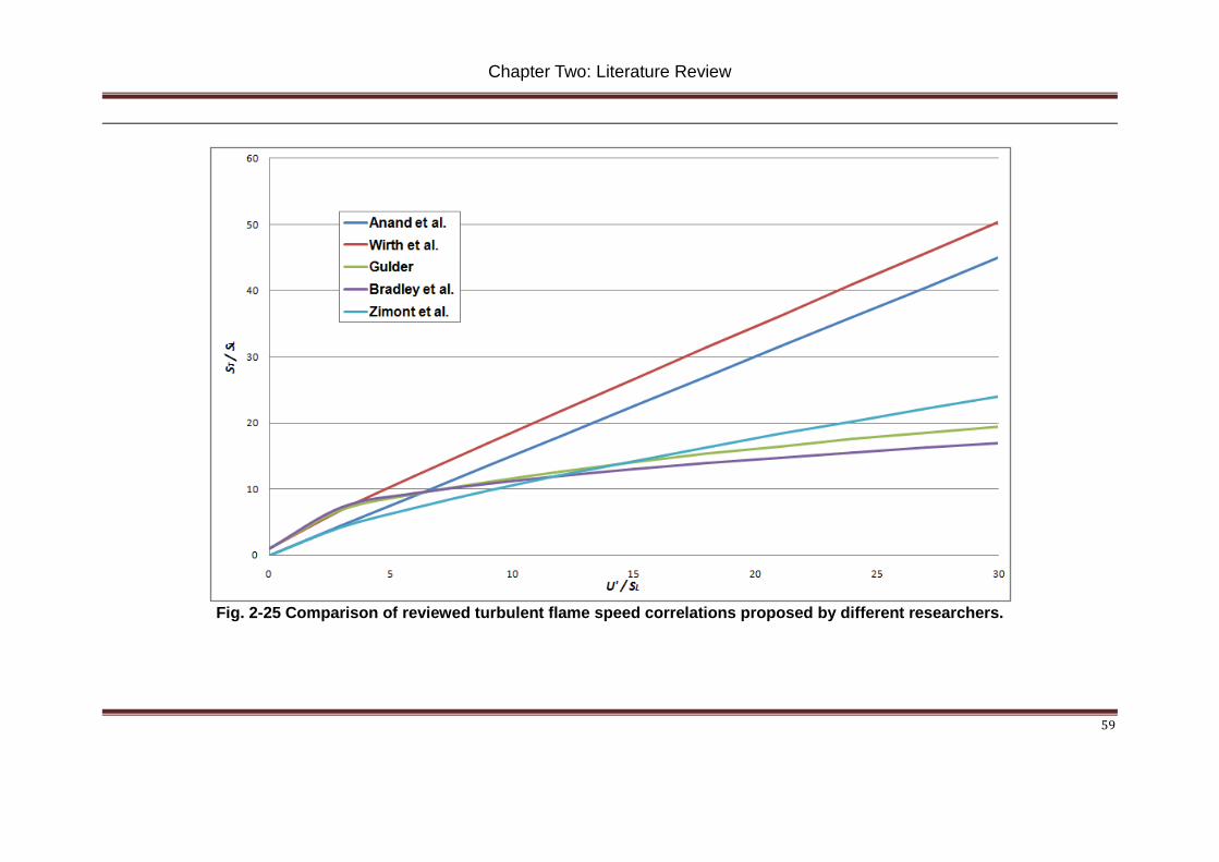
Chapter Two: Literature Review
59
Fig. 2-25 Comparison of reviewed turbulent flame speed correlations proposed by different researchers.
Chapter Two: Literature Review
60
2.4.3 Discussion on reviewed correlations
Anand and co-workers followed the original relation between 𝑺𝑻 and 𝑺𝑳 proposed
by Damkohler (1947) and derived a linear correlation between 𝑺𝑻 and 𝑺𝑳. However,
more recent experimental investigations of premixed turbulent flames, even at high
ratios 𝒖′/𝑺𝑳 in the flamelet regime, showed that the relation between ST/SL and
𝒖′/𝑺𝑳 is not linear and depends on fuel type. Some local influences are found to be
responsible for this effect (Wirth & Peters 1992).
Wirth and Peter developed a non-linear correlation using the G-equation concept.
the correlation has been validated on a near-production S.I. engine, which is
favourable for the current research. However, this correlation does not take into
account of the effect of flame stretch. Flame stretch has been found to be
particularly influential under lean-burn operating conditions, and have considerable
impact on the mean turbulent heat release intensity (Zimont & Polifke 1998).
Besides, Wirth and Peter’s correlation has only been validated against one type of
fuel which may make one to doubt its flexibility when some other available
correlations are validated against multiple fuels.
Zimont’s correlation has more solid and detailed theoretical background and is
claimed to be more robust and computationally efficient. This makes it favourable for
multi-dimensional simulations in complex geometries, e.g. internal combustion
engines. Zimont’s correlation has actually been adopted in the well-known
commercial CFD package FLUENT 6.3 for turbulent flames speed prediction, a
proof that it is sufficiently accurate and efficient. The only drawback of this
correlation, from the current author’s point of view, is the inclusion of the empirical
constant 𝑨. On the plus side, such inclusion makes the correlation very flexible, i.e.
𝑨 can be tuned to suit different fuels or operating conditions. But there is not
Chapter Two: Literature Review
61
implication that the variation of 𝑨 is related to either the combustion process or the
properties of the turbulence. This makes it difficult for an end-user to use values of
𝑨 other than those recommended by Zimont and co-workers, with a sound
theoretical ground.
The correlations proposed by Gulder and Bradley have very similar formation as
they both include the effect of turbulent Reynolds number. Flame stretch is
considered in both correlations and they have all been validated against multiple
types of fuels. The only difference, from the current author’s perspective, is that they
are biased towards different applications. Gulder’s correlation is applicable for three
turbulent combustion regimes, making it a very flexible tool for a wide range of
turbulent combustion. Bradley’s correlation, on the other hand, is based on the
two-eddy theory and therefore is focused on the wrinkled flamelet regime. Bradley
claimed that, by comparing to different theories of turbulent combustion, the
two-eddy theory is more satisfactory for combustion in higher levels of turbulence.
2.5 Chemical Kinetics
The equilibrium composition of a reactive mixture can be predicted by the
application of thermodynamic laws, In the case of that the chemical processes are
much faster compared with the other processes like diffusion, heat transfer, flow etc.
the thermodynamics alone allow the description of the system locally. In most cases,
though, chemical reactions occur on timescales comparable with those of the flow
and of the molecular transport processes. Therefore, information is needed about
the rates at which the chemical reactions proceed. For this purpose, chemical
kinetics has been investigated to study the rates of chemical processes in an effort
Chapter Two: Literature Review
62
to understand the factors that influence these rates and to develop theories that can
be used to predict chemical processes.
In the research of internal combustion engines, chemical kinetics fulfils the needs for
compact numerical models to represent hydrocarbon combustion and enables the
establishment and development of numerical models for the design and prediction
of practical engine systems. In general, chemical kinetics forms a link between
experimental observation and numerical interpretations of the combustion
processes in internal combustion engines.
2.5.1 Rate laws and rate constants
In this section, three types of reactions that are global, elementary and chain reactions
and the terms, equations and basic laws applied to describe each reaction type are
introduced.
Global reactions
The chemistry in fuel oxidation can be expressed by a global reaction mechanism.
Assuming that a mole of fuel reacts with combustion products, it yields:
𝟏𝟏𝒖𝑹𝒍 + 𝜶 𝑶𝑶𝒊𝒂𝒊𝑶𝑹𝑷 → 𝒃 𝑷𝑷𝑷𝒂𝒖𝒄𝒕𝒅 (2-29)
The fuel consumption rate can be expressed by:
𝒂[𝑬𝟏𝒖𝑹𝒍]𝒂𝒕
= 𝒌𝑮(𝑻) ∙ ⌈𝑬𝟏𝒖𝑹𝒍⌉𝒏 ∙ [𝑬𝑶𝑶𝒊𝒂𝒊𝑶𝑹𝑷]𝒎 (2-30)
where [𝑬𝒊] denotes the molar concentration of the ith species in the mixture. 𝒌𝑮(𝑻)
is the global rate coefficient and is a strong function of temperature. The minus sign
indicates that fuel concentration decreases with time. The exponent n and m relate to
Chapter Two: Literature Review
63
the reaction order.
Use of global reactions to express a chemical reaction system is frequently a ‘black
box’ approach by providing the input-to-out perspective to the chemical process,
which is not capable of providing a basis for understanding what is actually happening
chemically in a system. The chemical equation Eq. 2-29 indicates that the oxidation
process of the fuel is a one-step and instantaneous process. In reality, it is however a
much more complex and sequential process. This process involves the breaking and
formation of chemical bonds and production and destruction of intermediate species.
A global equation consequently is not adequate to describe a chemical process in
details, so a collection of elementary reactions has to be used to depict a chemical
process, which will be considered in the following section.
Elementary reactions
Elementary reactions express how actual molecules or ions react with each other.
The equation in an elementary reaction represents the reaction at the molecular
level rather than at a global point of view. Based on the number s of the molecules
involved, elementary reactions are categorised into three types: unimolecular
reactions, bimolecular reactions and trimolecular reactions (Liu 2010):
Unimolecular reactions
Unimolecular reactions describe the process that a molecule or ion decomposes
itself. They are always first order reactions and can be expressed in the following
form:
𝑨 → 𝒑𝑷𝑷𝒂𝒖𝒄𝒕𝒅 (2-31)
Chapter Two: Literature Review
64
The reaction rate of above reaction is directly proportional to the concentration of the
reactant, 𝑨:
𝒂[𝑨]𝒂𝒕
= −𝒌 ∙ [𝑨] (2-32)
where 𝒌 represents the rate coefficient.
Bimolecular reactions
Most elementary reactions involved in combustion are bimolecular. In a bimolecular
reaction two molecules collide and react with each other and form two different
molecules:
𝑫𝑨 + 𝒃𝑩 → 𝒄𝑪 + 𝒂𝑫 (2-33)
where 𝑫, 𝒃, 𝒄 and 𝒂 are stoichiometric coefficients. The reaction rate of this
reaction is calculated by multiplying the reaction rate constants by the concentration
of each of the reactants:
𝟏𝑫
𝒂[𝑨]𝒂𝒕
= 𝟏𝒃𝒂[𝑩]𝒂𝒕
= −𝟏𝒄𝒂[𝑪]𝒂𝒕
= −𝟏𝒂𝒂[𝑫]𝒂𝒕
= −𝒌 ∙ [𝑨] ∙ [𝑩] (2-34)
The negative reaction rates indicate that the species are being consumed.
Trimolecular reactions
A trimolecular reaction involves the collisions amongst three molecules. The general
form of a trimolecular reaction is:
𝑨 + 𝑩 + 𝑴 → 𝑪 + 𝑴 (2-35)
and the its reaction rate is expressed as:
Chapter Two: Literature Review
65
𝒂[𝑨]𝒂𝒕
= −𝒌 ∙ [𝑨] ∙ [𝑩] ∙ [𝑴] (2-36)
where 𝑴 can be any molecule and is often referred to as the third body.
Reaction rates of elementary reactions
It has been observed from both kinetic theories of gases and experiments that the
rate constant, 𝒌 , for an elementary reaction is an exponential function of
temperature and is in the form of the Arrhenius equation:
𝒌(𝑻) = 𝑨 ∙ 𝑻𝒃 ∙ 𝑹𝑶𝒑 �− 𝑬𝑨𝑹𝒖𝑻
� (2-37)
where 𝑨 is the pre-exponential factor and 𝑬𝑨 is the activation energy of the
reaction which represents the energy level required to activate the chemical bonds
break-up and rearrangement processes. These two constants are determined
experimentally.
Chain reactions
Most gas-phase chemical reactions are initiated at low concentrations by the
formation of an extremely reactive species that sets off a series of reactions leading
to a self-amplifying and self-sustaining chain of chemical events. Such process is
referred to as a chain reaction. Chain reactions occur after a short induction period
that allows the formation and accumulation of the reactive species.
The sequence of a reaction chain can be typically divided into four stages:
Initiation: A highly reactive intermediates is formed usually through the action of an
agent such as light, heat or a catalyst. These intermediates can be in the form of an
atom, an ion or a neutral molecular fragment.
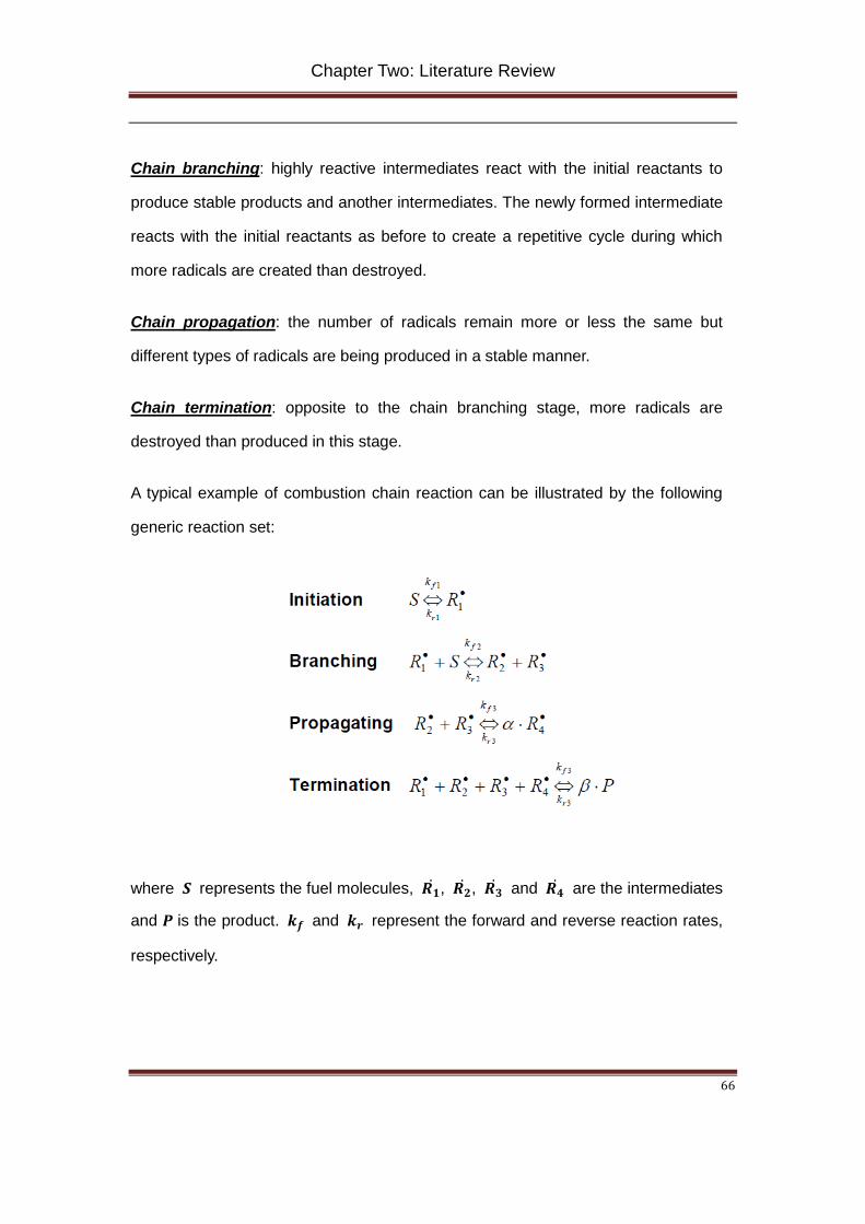
Chapter Two: Literature Review
66
Chain branching: highly reactive intermediates react with the initial reactants to
produce stable products and another intermediates. The newly formed intermediate
reacts with the initial reactants as before to create a repetitive cycle during which
more radicals are created than destroyed.
Chain propagation: the number of radicals remain more or less the same but
different types of radicals are being produced in a stable manner.
Chain termination: opposite to the chain branching stage, more radicals are
destroyed than produced in this stage.
A typical example of combustion chain reaction can be illustrated by the following
generic reaction set:
where 𝑺 represents the fuel molecules, 𝑹�̇�, 𝑹�̇�, 𝑹�̇� and 𝑹�̇� are the intermediates
and P is the product. 𝒌𝒇 and 𝒌𝑷 represent the forward and reverse reaction rates,
respectively.
Chapter Two: Literature Review
67
Reaction rates of chain reactions
Based on the elementary reaction rates expressed using Eq. 2-35, 2-36 and 2-37,
the net production or destruction rates of any species involved in a series of chain
reaction can mathematically expressed. The net production rate of 𝑹�̇� is the sum of
all elementary rates producing 𝑹�̇� minus the sum of all elementary rates destroying
𝑹�̇�:
𝐝�𝑹�̇��𝐝𝐭
= 𝐤𝐟𝟏[𝐒] + 𝐤𝐟𝟐�𝑹�̇���𝑹�̇��+ 𝒌𝒇𝟒[𝑷]𝜷 − 𝐤𝐫𝟏�𝐑�̇�� − 𝐤𝐫𝟐�𝐑�̇��[𝐒]−
𝐤𝐟𝟒�𝐑�̇���𝐑�̇���𝐑�̇���𝐑�̇�� (2-38)
The same applies to 𝑹�̇�, 𝑹�̇� and 𝑹�̇� and after obtaining expressions for each
species it yields a system of first-order ordinary differential equation that describes
the evolution of the chemical system:
𝒂[𝑬𝒊](𝒕)𝒂𝒕
= 𝒇 ([𝑬𝟏](𝒕), [𝑬𝟐](𝒕), … , [𝑬𝒏](𝒕)) (2-39)
With known initial conditions:
[𝑬𝒊](𝒕 = 𝟏) = [𝑬𝒊]𝟏 (2-40)
Together with the conservation equations of mass and energy the set of equations
can be numerically integrated using computerized methods. It should be noted that
such chemical system has an important feature of being stiff, which means some of
the variables are changing rapidly while some are changing very slowly. The
character of stiffness of a system of ODEs requires more complex numerical
integration methods, i.e., Backward Euler method, to achieve reliable results.
2.5.2 Chemical kinetic combustion models
Chemical kinetics mechanisms are very useful tools in the prediction of autoignition
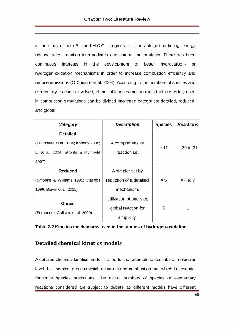
Chapter Two: Literature Review
68
in the study of both S.I. and H.C.C.I. engines, i.e., the autoignition timing, energy
release rates, reaction intermediates and combustion products. There has been
continuous interests in the development of better hydrocarbon- or
hydrogen-oxidation mechanisms in order to increase combustion efficiency and
reduce emissions (O Conaire et al. 2004). According to the numbers of species and
elementary reactions involved, chemical kinetics mechanisms that are widely used
in combustion simulations can be divided into three categories: detailed, reduced,
and global:
Category Description Species Reactions
Detailed
(O Conaire et al. 2004; Konnov 2008;
Li et al. 2004; Strohle & Myhrvold
2007)
A comprehensive
reaction set ≈ 11 ≈ 20 to 21
Reduced
(Smooke & Williams 1995; Vlachos
1996; Boivin et al. 2011)
A simpler set by
reduction of a detailed
mechanism.
≈ 5 ≈ 4 to 7
Global
(Fernández-Galisteo et al. 2009)
Utilization of one-step
global reaction for
simplicity.
3 1
Table 2-2 Kinetics mechanisms used in the studies of hydrogen-oxidation.
Detailed chemical kinetics models
A detailed chemical kinetics model is a model that attempts to describe at molecular
level the chemical process which occurs during combustion and which is essential
for trace species predictions. The actual numbers of species or elementary
reactions considered are subject to debate as different models have different
Chapter Two: Literature Review
69
focuses (Simmie 2003). Many researchers use truncated or skeletal mechanisms
that completely neglect some intermediates or do not differentiate between various
quantum state of one compound.
For decades, the study and development of chemical kinetics mechanisms have
been concentrated on single sets of experimental data obtained from shock tubes,
flow reactors or rapid compression machines (O Conaire et al. 2004). Schott and
Kinsey (1958) studied the formation of OH radicals in hydrogen-air combustion
under 1atm and a wide temperature range between 1085-2700K in a shock tube.
Five chain branching reactions from a detailed mechanism were shown to have
significant influence on the oxidation of hydrogen and its ignition delay. Skinner and
Ringrose (Konnov 2008) performed measurements in shock tube with extended
pressure up to 5atm and found similar results. Chen et al. (1984) and Slack (1977)
measured the ignition delay of hydrogen-air mixture under similar temperature and
pressure range but different levels of dilution using inert gas Argon. However, the
reliance on just one set of experimental data is criticized recently (Smith 2002) who
asserts uncertainty limits on individual reaction rate constants produce a parameter
space for imprecise predictions of key combustion properties such as the flame
speed and the ignition delay. Following Smith’s critics some researchers started to
develop and validate their chemical kinetics mechanism against a wider range of
experimental results that were obtained by various experimental techniques.
Several detailed hydrogen oxidation mechanisms have been proposed over the
years. The motivation of such continuous development is the substantial progress
made in accurate measurement of the elementary reaction rates and
thermodynamic properties as well as in measurement of the integral combustion
characteristics such as burning velocities, ignition delays, and product formation
during slow oxidation (Konnov 2008). Others (Mueller et al. 1999) proposed a
Chapter Two: Literature Review
70
detailed hydrogen oxidation mechanism using only a flow reactor over the
temperature range of 850-1040K, at equivalence ratio between 0.3 and 1.0 and
pressures between 0.3 to 17.5atm. By taking advantages of a expanded database
and improved rate constants of H + O2 (+ N2) = HO2 (+ N2), HO2 + OH = H2O + O2,
and HO2 + HO2 = H2O2 + O2, the proposed mechanism was in better agreement
with experimental results. Similarly, Davies et al. (2003) improved the detailed
H2/CO mechanism they proposed previously by adopting new rate constants for the
important reaction H + O2 + M = HO2 +M and new thermodynamic data for OH
radicals. Based previous works of (Konnov 2008),(Hughes et al. n.d.) and the
GRI-mech (Smith et al. n.d.), Conaire (2004) developed a detailed hydrogen
oxidation mechanism which was validated against experimental results obtained
from multiple sources including shock tube, flow reactor, freely propagating flames
and burner-stabilized flames. With increased attention paid to the suitability to
simulations under high pressure, i.e. internal combustion engines, Conaire validated
the mechanism over the range of 298-2700K, 0.05-87atm and Ф = 0.2-6. By
applying a pressure-dependent rate constant for H + OH + M = H2O + M Conaire’s
mechanism achieved better overall agreement to a wide range of physical
conditions and greater consistency over existing hydrogen oxidation mechanism.
Reduced chemical kinetics models
As the numbers of species and reactions required to describe a chemical reaction
system in details increases, the demand on computational power becomes the
major huddle that prevents detailed chemical kinetics models to be adopted in the
simulation of practical combustion applications, i.e. internal combustion engines.
The situation gets even worse when detailed chemical kinetics models are coupled
with multi-dimensional CFD calculations (Ra & Reitz 2008). Recent detailed
Chapter Two: Literature Review
71
n-heptane oxidation mechanism developed by Curran et al. (1998) contains 560
species and 2539 elementary reaction. An iso-octane oxidation mechanism by the
same author later (Curran et al. 2002) contains 857 species and 3606 elementary
reactions. It is still too expensive to use detailed chemical kinetics mechanisms in
engine simulation with multidimensional CFD codes, even with modern
high-performance super computers. Therefore methods of simplification on detailed
chemical kinetics models are required. The simplified mechanisms are often
referred to as reduced chemical kinetics mechanisms. The reduced mechanisms
should retain all the critical fuel chemistry predicted by detailed mechanisms, but
with much improve computational efficiency. The extent of comprehensiveness of
the reduced mechanisms depends on the available computational resources and
the information required from the simulation.
Various theoretical methods of simplification have been proposed. Maas et al. (2000)
proposed a reduction method based on the Intrinsic Low-Dimensional Manifolds
(ILMDs). The dynamical behaviours of the chemical systems are well reproduced,
independent on the fuel type considered. Simpler reaction mechanisms of Syngas,
methane, iso-octane, n-dodecane are achieved. By analysing the reaction rates,
Law et al. (1998) developed a reduced methane oxidation mechanism that consists
of 16 species and 12 lumped steps. The reduction was carried out on GRI-Mech 1.2
which consists of 31 species and 175 elementary reactions. The reduced
mechanism retained the capabilities of predicting a wide range of combustion
phenomena with extensive thermo-dynamical parametric variations.
In terms of applications in engine combustion simulations, Reitz et al. (2008)
proposed a reduced oxidation mechanism by combing reduced n-heptane and
iso-octane oxidation mechanisms. By adopting the reduced mechanism into a
multi-dimensional CFD H.C.C.I. engine model and D.I. diesel engine model, the
Chapter Two: Literature Review
72
mechanism was proven to produce reliable predictions on engine combustion as
well as improved computational efficiency over detailed mechanism. Tanaka et al.
(2003) have developed a reduced oxidation mechanism for gasoline, as a mixture of
n-heptane and iso-octane, as shown in Fig. 2-26. The mechanism which consists of
32 species and 55 elementary reactions takes into account of the effects of wall heat
transfer on the adiabatic core gas temperature by adding then displacement volume
of the laminar boundary layer to the cylinder volume. Chemical interactions between
n-heptane and iso-octane are also included. Tanaka’s mechanism successfully
predicts the two-stage heat release of heavy hydrocarbons which involves low and
high temperature cycles followed by a chain explosion.
Global chemical kinetics models
Global chemical kinetics mechanisms describe the chemistry in terms of a few of the
principle reactants and products in one or more function steps (Zheng 2005). The
motivation of developing a global chemical kinetics mechanism is the application in
combustion simulations that required considerable computational resource, i.e.
multi-dimensional engine simulation.
The chain reaction theory still applies in the construction of global mechanisms. In
general, the high temperature chemistry is described by one or two reaction steps
and the other reactions are used to represent the low and intermediate temperature
chemistry (Liu 2010). The drawback of global mechanisms is its inability of
predicting the post-ignition reactions and the combustion intermediates. Therefore,
the usage of global mechanisms is limited to the prediction of pre-ignition
behaviours, e.g. ignition delay.

Chapter Two: Literature Review
73
Fig. 2-26 Illustration of the reduced chemistry of the mixture of n-heptane and
iso-octane as developed by Tanaka et al. (Tanaka et al. 2003).
Westbrook et al. (1996) developed a one-step global mechanism of hydrogen
oxidation:
H2 + 1/2 O2 = H2O
where the overall reaction rate is expressed as:
𝒌 = 𝟏.𝟔 𝑶 𝟏𝟏𝟏𝟑 ∙ 𝑬𝑬𝑷 �−𝟏𝟏𝟔𝟏𝟒𝑲𝑻
� ∙ [𝑯𝟐]𝟏.𝟏 ∙ [𝑶𝟐]𝟏.𝟓 (2-41)
In laminar flame speed simulations, the global mechanism was only reliable in a
limited range of equivalence ratio between 0.55 and 1.1. Predictions outside this
Chapter Two: Literature Review
74
range was considered poor and unreliable. The poor prediction was attributed to the
chemical and thermal structure changes in the flame as the stoichiometry varies
which could not be properly accounted for in the global mechanism.
Chapter Three: Hydrogen-Air Spherical Flame Instabilities
75
Chapter Three: Hydrogen-Air Spherical Flame Instabilities
This chapter focuses on the systematic studies of the onset of hydrogen-air spherical
flame instabilities which is defined by the critical radius, and its relationships with
equivalence ratio, temperature and pressure. The aim of the current chapter’s
research is to:
(1) Experimentally identify the critical radius for the onset of instabilities of
hydrogen-air flames, and,
(2) Systematically examine the effects of temperature, pressure and fuel-air
equivalence ratio on the variation of the critical radius.
3.1 Cellular flame instabilities
According to the mechanism that triggers the instabilities of laminar flames two main
kinds of instabilities are defined and studied: unequal diffusion instability and
hydrodynamic instability (Bradley et al. 1996; Tang et al. 2009; Aung et al. 1998; Hu et
al. 2009; Aung et al. 1997; Kwon & Faeth 2001; Bradley et al. 1998; Sun et al. 2012;
Bradley & Harper 1994). A third category, buoyant instability, caused by gravitational
effect, can also be found in previous research (Vu et al. 2011). It is often neglected as
its effect on rapidly propagating flames is minor compared to the other two categories
of instabilities.
3.1.1 Unequal diffusion instabilities
The unequal diffusion instability is sometimes referred to as thermal-diffusive
instability. During the flame propagation process, both mass and thermal diffusions
exist across the flame surface. The energy ratio of the two kinds of diffusion is
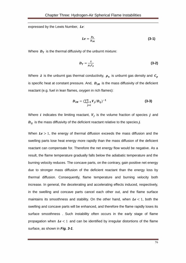
Chapter Three: Hydrogen-Air Spherical Flame Instabilities
76
expressed by the Lewis Number, 𝑳𝑳:
𝑳𝑳 = 𝑫𝑻𝑫𝒊𝒊
(3-1)
Where 𝑫𝑻 is the thermal diffusivity of the unburnt mixture:
𝑫𝑻 = 𝝀𝝆𝒖𝑪𝒑
(3-2)
Where 𝝀 is the unburnt gas thermal conductivity, 𝝆𝒖 is unburnt gas density and 𝑪𝒑
is specific heat at constant pressure. And, 𝑫𝒊𝒊 is the mass diffusivity of the deficient
reactant (e.g. fuel in lean flames, oxygen in rich flames):
𝑫𝒊𝒊 = (∑ 𝑽𝒋/𝑫𝒊𝒋𝒏𝒋=𝟏𝒋≠𝒊
)−𝟏 (3-3)
Where 𝒊 indicates the limiting reactant, 𝑽𝒋 is the volume fraction of species 𝒋 and
𝑫𝒊𝒋 is the mass diffusivity of the deficient reactant relative to the species 𝒋.
When 𝑳𝑳 > 1, the energy of thermal diffusion exceeds the mass diffusion and the
swelling parts lose heat energy more rapidly than the mass diffusion of the deficient
reactant can compensate for. Therefore the net energy flow would be negative. As a
result, the flame temperature gradually falls below the adiabatic temperature and the
burning velocity reduces. The concave parts, on the contrary, gain positive net energy
due to stronger mass diffusion of the deficient reactant than the energy loss by
thermal diffusion. Consequently, flame temperature and burning velocity both
increase. In general, the decelerating and accelerating effects induced, respectively,
in the swelling and concave parts cancel each other out, and the flame surface
maintains its smoothness and stability. On the other hand, when 𝑳𝑳 < 1, both the
swelling and concave parts will be enhanced, and therefore the flame rapidly loses its
surface smoothness . Such instability often occurs in the early stage of flame
propagation when 𝑳𝑳 < 1 and can be identified by irregular distortions of the flame
surface, as shown in Fig. 3-1.
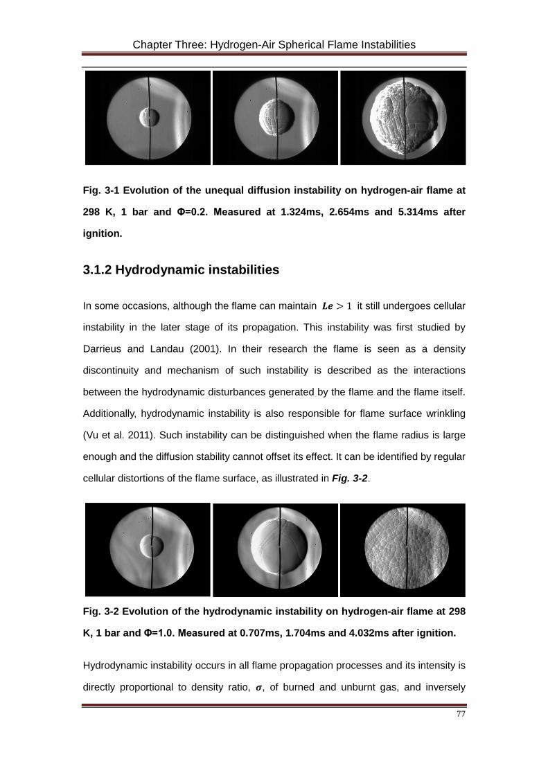
Chapter Three: Hydrogen-Air Spherical Flame Instabilities
77
Fig. 3-1 Evolution of the unequal diffusion instability on hydrogen-air flame at
298 K, 1 bar and Φ=0.2. Measured at 1.324ms, 2.654ms and 5.314ms after
ignition.
3.1.2 Hydrodynamic instabilities
In some occasions, although the flame can maintain 𝑳𝑳 > 1 it still undergoes cellular
instability in the later stage of its propagation. This instability was first studied by
Darrieus and Landau (2001). In their research the flame is seen as a density
discontinuity and mechanism of such instability is described as the interactions
between the hydrodynamic disturbances generated by the flame and the flame itself.
Additionally, hydrodynamic instability is also responsible for flame surface wrinkling
(Vu et al. 2011). Such instability can be distinguished when the flame radius is large
enough and the diffusion stability cannot offset its effect. It can be identified by regular
cellular distortions of the flame surface, as illustrated in Fig. 3-2.
Fig. 3-2 Evolution of the hydrodynamic instability on hydrogen-air flame at 298
K, 1 bar and Φ=1.0. Measured at 0.707ms, 1.704ms and 4.032ms after ignition.
Hydrodynamic instability occurs in all flame propagation processes and its intensity is
directly proportional to density ratio, 𝝈, of burned and unburnt gas, and inversely
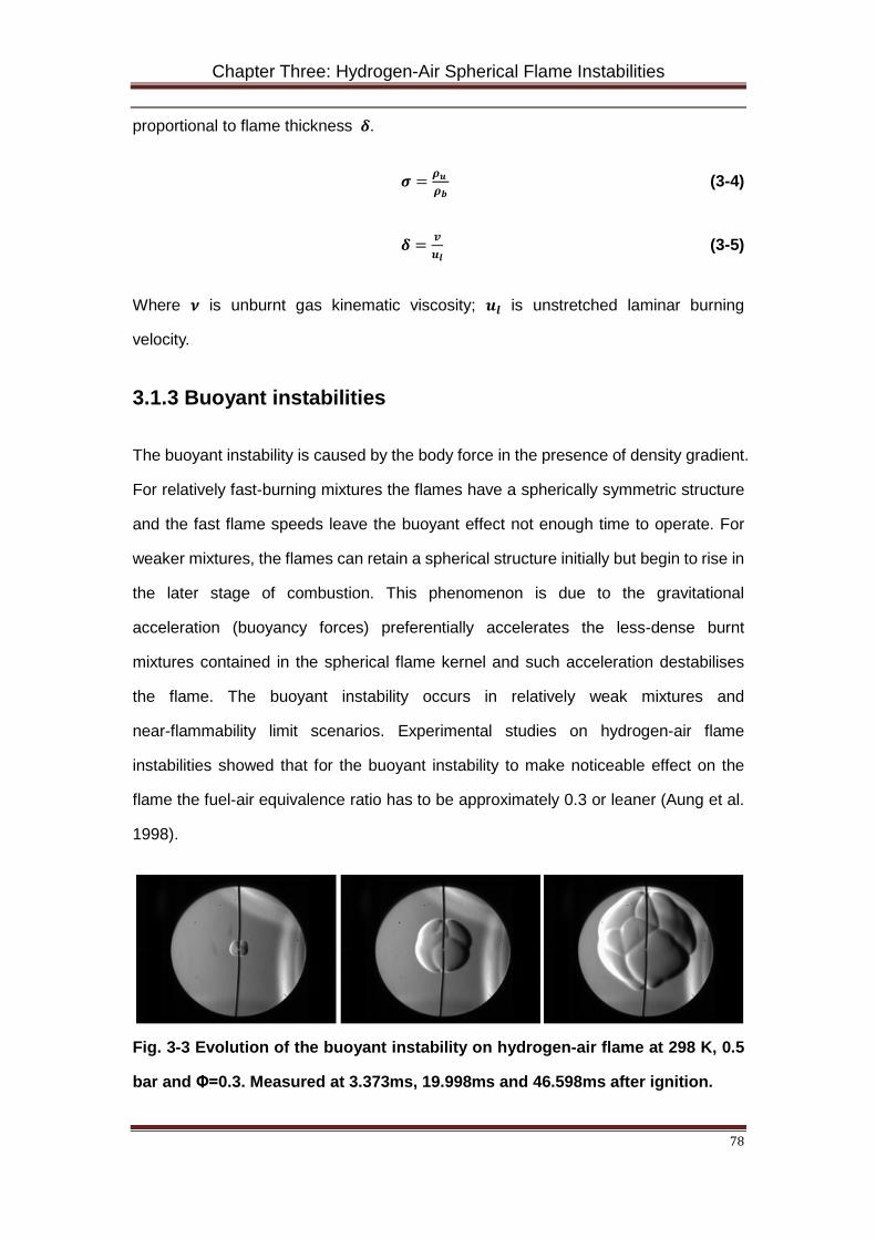
Chapter Three: Hydrogen-Air Spherical Flame Instabilities
78
proportional to flame thickness 𝜹.
𝝈 = 𝝆𝒖 𝝆𝒃
(3-4)
𝜹 = 𝒗𝒖𝒍
(3-5)
Where 𝝂 is unburnt gas kinematic viscosity; 𝒖𝒍 is unstretched laminar burning
velocity.
3.1.3 Buoyant instabilities
The buoyant instability is caused by the body force in the presence of density gradient.
For relatively fast-burning mixtures the flames have a spherically symmetric structure
and the fast flame speeds leave the buoyant effect not enough time to operate. For
weaker mixtures, the flames can retain a spherical structure initially but begin to rise in
the later stage of combustion. This phenomenon is due to the gravitational
acceleration (buoyancy forces) preferentially accelerates the less-dense burnt
mixtures contained in the spherical flame kernel and such acceleration destabilises
the flame. The buoyant instability occurs in relatively weak mixtures and
near-flammability limit scenarios. Experimental studies on hydrogen-air flame
instabilities showed that for the buoyant instability to make noticeable effect on the
flame the fuel-air equivalence ratio has to be approximately 0.3 or leaner (Aung et al.
1998).
Fig. 3-3 Evolution of the buoyant instability on hydrogen-air flame at 298 K, 0.5
bar and Φ=0.3. Measured at 3.373ms, 19.998ms and 46.598ms after ignition.
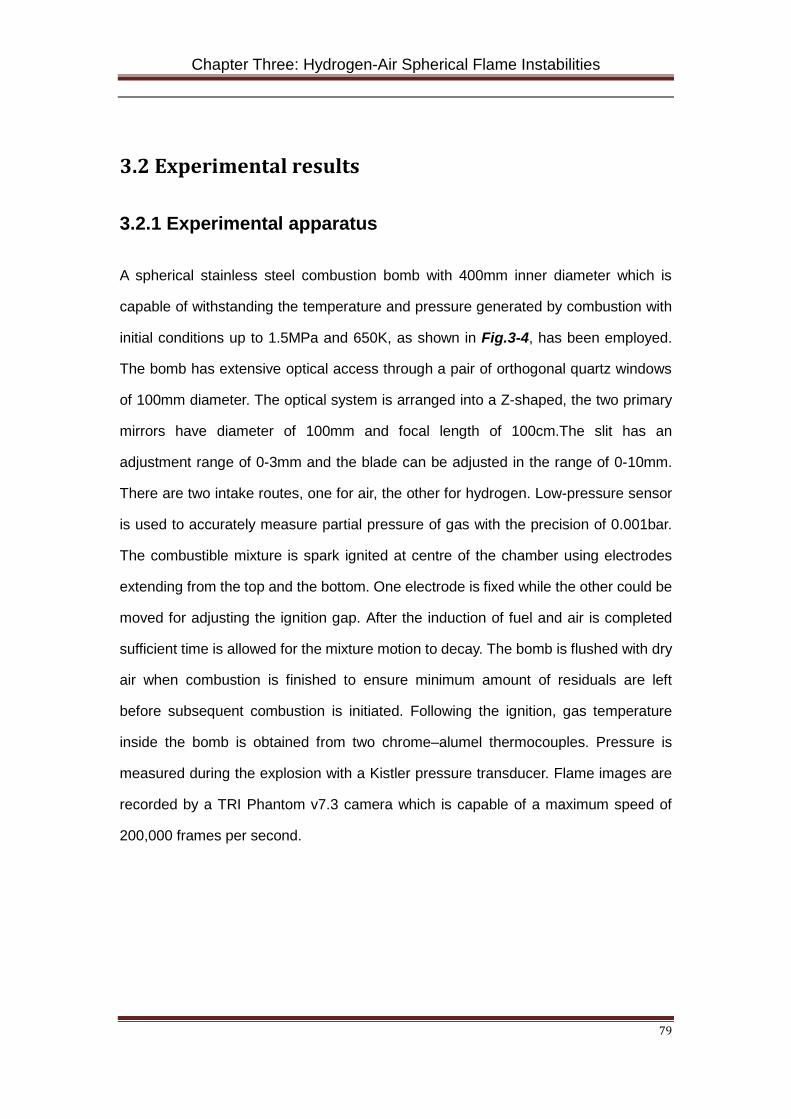
Chapter Three: Hydrogen-Air Spherical Flame Instabilities
79
3.2 Experimental results
3.2.1 Experimental apparatus
A spherical stainless steel combustion bomb with 400mm inner diameter which is
capable of withstanding the temperature and pressure generated by combustion with
initial conditions up to 1.5MPa and 650K, as shown in Fig.3-4, has been employed.
The bomb has extensive optical access through a pair of orthogonal quartz windows
of 100mm diameter. The optical system is arranged into a Z-shaped, the two primary
mirrors have diameter of 100mm and focal length of 100cm.The slit has an
adjustment range of 0-3mm and the blade can be adjusted in the range of 0-10mm.
There are two intake routes, one for air, the other for hydrogen. Low-pressure sensor
is used to accurately measure partial pressure of gas with the precision of 0.001bar.
The combustible mixture is spark ignited at centre of the chamber using electrodes
extending from the top and the bottom. One electrode is fixed while the other could be
moved for adjusting the ignition gap. After the induction of fuel and air is completed
sufficient time is allowed for the mixture motion to decay. The bomb is flushed with dry
air when combustion is finished to ensure minimum amount of residuals are left
before subsequent combustion is initiated. Following the ignition, gas temperature
inside the bomb is obtained from two chrome–alumel thermocouples. Pressure is
measured during the explosion with a Kistler pressure transducer. Flame images are
recorded by a TRI Phantom v7.3 camera which is capable of a maximum speed of
200,000 frames per second.
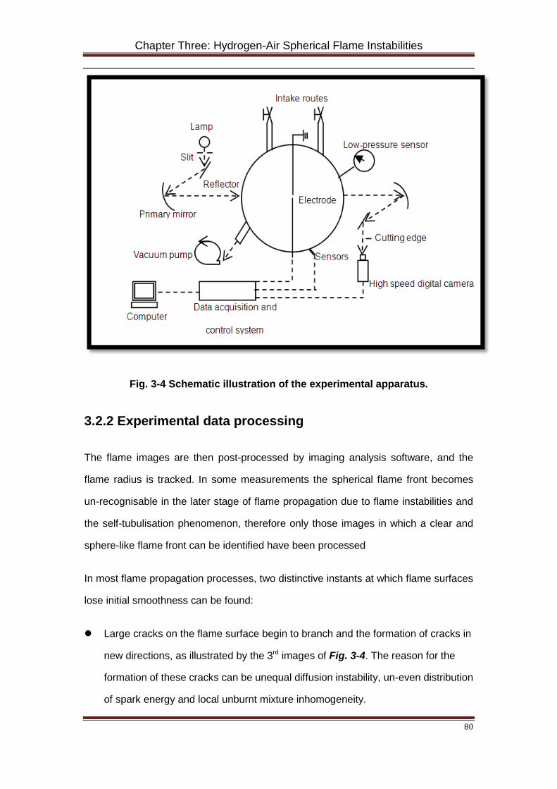
Chapter Three: Hydrogen-Air Spherical Flame Instabilities
80
Fig. 3-4 Schematic illustration of the experimental apparatus.
3.2.2 Experimental data processing
The flame images are then post-processed by imaging analysis software, and the
flame radius is tracked. In some measurements the spherical flame front becomes
un-recognisable in the later stage of flame propagation due to flame instabilities and
the self-tubulisation phenomenon, therefore only those images in which a clear and
sphere-like flame front can be identified have been processed
In most flame propagation processes, two distinctive instants at which flame surfaces
lose initial smoothness can be found:
Large cracks on the flame surface begin to branch and the formation of cracks in
new directions, as illustrated by the 3rd images of Fig. 3-4. The reason for the
formation of these cracks can be unequal diffusion instability, un-even distribution
of spark energy and local unburnt mixture inhomogeneity.
Chapter Three: Hydrogen-Air Spherical Flame Instabilities
81
Sudden and spontaneous appearance of a large number of small cells over the
entire flame surface (the 4th image of Fig. 3-5). The characteristic length scale of
such cells is significantly smaller than that of those large cracks. The appearance
of these small cells is caused by hydrodynamic instability.
Fig. 3-5 Serial images of propagation process of hydrogen-air flame at 298 K, 1
bar, Φ=0.8. Measurement times are (from top left to bottom right): 0.382ms,
0.771ms, 1.50ms, 3.01ms, 3.48ms and 4.56ms.
In the analysis below, the second instant will be used primarily as the onset of flame
instability, unless significant unequal diffusion instability can be identified earlier. The
reason being: firstly, unlike the unequal diffusion instability, hydrodynamic instability
occurs in almost all flame propagations. Secondly, compared to the growth and
branching of large cracks, hydrodynamic instability occurs with very high intensity, i.e.
small cells grow across the entire flame surface spontaneously, making it relatively
easier to accurately identify the exact onset timing. Additionally, values of 𝑳𝑳, σ and δ
are calculated based on initial temperature, pressure and equivalence ratio prior to
ignition.
.
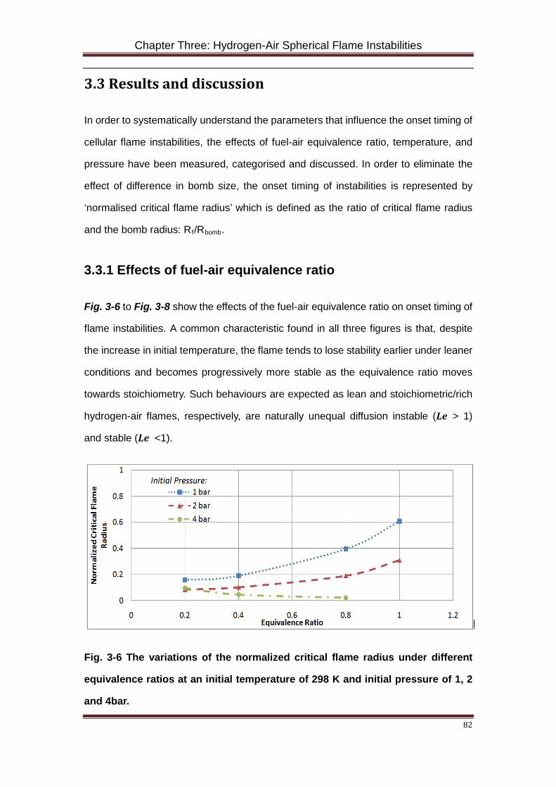
Chapter Three: Hydrogen-Air Spherical Flame Instabilities
82
3.3 Results and discussion
In order to systematically understand the parameters that influence the onset timing of
cellular flame instabilities, the effects of fuel-air equivalence ratio, temperature, and
pressure have been measured, categorised and discussed. In order to eliminate the
effect of difference in bomb size, the onset timing of instabilities is represented by
‘normalised critical flame radius’ which is defined as the ratio of critical flame radius
and the bomb radius: Rf/Rbomb.
3.3.1 Effects of fuel-air equivalence ratio
Fig. 3-6 to Fig. 3-8 show the effects of the fuel-air equivalence ratio on onset timing of
flame instabilities. A common characteristic found in all three figures is that, despite
the increase in initial temperature, the flame tends to lose stability earlier under leaner
conditions and becomes progressively more stable as the equivalence ratio moves
towards stoichiometry. Such behaviours are expected as lean and stoichiometric/rich
hydrogen-air flames, respectively, are naturally unequal diffusion instable (𝑳𝑳 > 1)
and stable (𝑳𝑳 <1).
Fig. 3-6 The variations of the normalized critical flame radius under different
equivalence ratios at an initial temperature of 298 K and initial pressure of 1, 2
and 4bar.
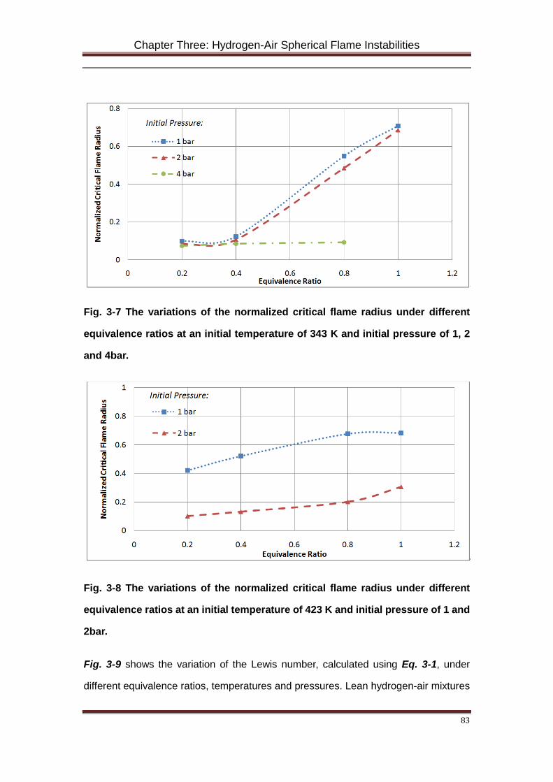
Chapter Three: Hydrogen-Air Spherical Flame Instabilities
83
Fig. 3-7 The variations of the normalized critical flame radius under different
equivalence ratios at an initial temperature of 343 K and initial pressure of 1, 2
and 4bar.
Fig. 3-8 The variations of the normalized critical flame radius under different
equivalence ratios at an initial temperature of 423 K and initial pressure of 1 and
2bar.
Fig. 3-9 shows the variation of the Lewis number, calculated using Eq. 3-1, under
different equivalence ratios, temperatures and pressures. Lean hydrogen-air mixtures
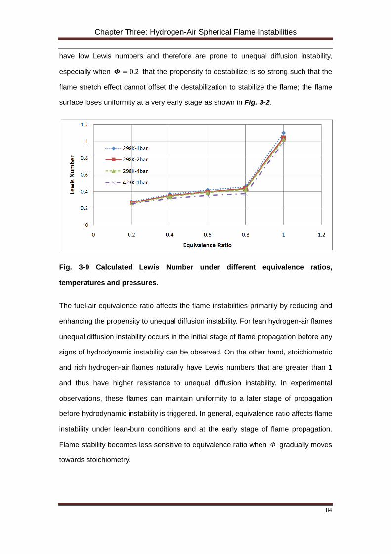
Chapter Three: Hydrogen-Air Spherical Flame Instabilities
84
have low Lewis numbers and therefore are prone to unequal diffusion instability,
especially when 𝜱 = 0.2 that the propensity to destabilize is so strong such that the
flame stretch effect cannot offset the destabilization to stabilize the flame; the flame
surface loses uniformity at a very early stage as shown in Fig. 3-2.
Fig. 3-9 Calculated Lewis Number under different equivalence ratios,
temperatures and pressures.
The fuel-air equivalence ratio affects the flame instabilities primarily by reducing and
enhancing the propensity to unequal diffusion instability. For lean hydrogen-air flames
unequal diffusion instability occurs in the initial stage of flame propagation before any
signs of hydrodynamic instability can be observed. On the other hand, stoichiometric
and rich hydrogen-air flames naturally have Lewis numbers that are greater than 1
and thus have higher resistance to unequal diffusion instability. In experimental
observations, these flames can maintain uniformity to a later stage of propagation
before hydrodynamic instability is triggered. In general, equivalence ratio affects flame
instability under lean-burn conditions and at the early stage of flame propagation.
Flame stability becomes less sensitive to equivalence ratio when 𝛷 gradually moves
towards stoichiometry.
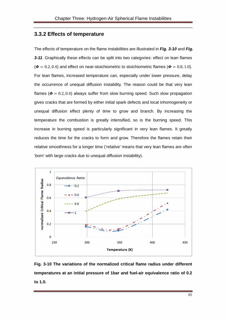
Chapter Three: Hydrogen-Air Spherical Flame Instabilities
85
3.3.2 Effects of temperature
The effects of temperature on the flame instabilities are illustrated in Fig. 3-10 and Fig.
3-11. Graphically these effects can be split into two categories: effect on lean flames
(𝜱 = 0.2, 0.4) and effect on near-stoichiometric to stoichiometric flames (𝜱 = 0.8, 1.0).
For lean flames, increased temperature can, especially under lower pressure, delay
the occurrence of unequal diffusion instability. The reason could be that very lean
flames (𝜱 = 0.2, 0.4) always suffer from slow burning speed. Such slow propagation
gives cracks that are formed by either initial spark defects and local inhomogeneity or
unequal diffusion effect plenty of time to grow and branch. By increasing the
temperature the combustion is greatly intensified, so is the burning speed. This
increase in burning speed is particularly significant in very lean flames. It greatly
reduces the time for the cracks to form and grow. Therefore the flames retain their
relative smoothness for a longer time (‘relative’ means that very lean flames are often
‘born’ with large cracks due to unequal diffusion instability).
Fig. 3-10 The variations of the normalized critical flame radius under different
temperatures at an initial pressure of 1bar and fuel-air equivalence ratio of 0.2
to 1.0.
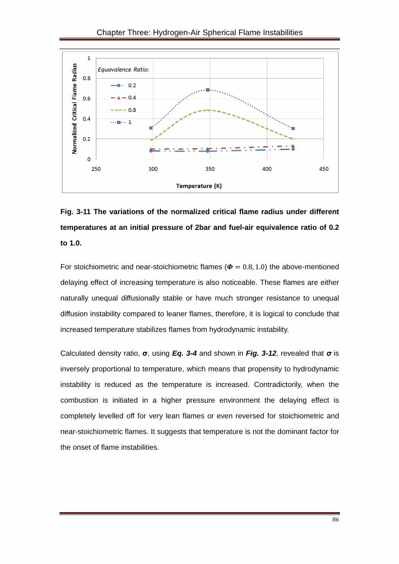
Chapter Three: Hydrogen-Air Spherical Flame Instabilities
86
Fig. 3-11 The variations of the normalized critical flame radius under different
temperatures at an initial pressure of 2bar and fuel-air equivalence ratio of 0.2
to 1.0.
For stoichiometric and near-stoichiometric flames (𝜱 = 0.8, 1.0) the above-mentioned
delaying effect of increasing temperature is also noticeable. These flames are either
naturally unequal diffusionally stable or have much stronger resistance to unequal
diffusion instability compared to leaner flames, therefore, it is logical to conclude that
increased temperature stabilizes flames from hydrodynamic instability.
Calculated density ratio, σ, using Eq. 3-4 and shown in Fig. 3-12, revealed that σ is
inversely proportional to temperature, which means that propensity to hydrodynamic
instability is reduced as the temperature is increased. Contradictorily, when the
combustion is initiated in a higher pressure environment the delaying effect is
completely levelled off for very lean flames or even reversed for stoichiometric and
near-stoichiometric flames. It suggests that temperature is not the dominant factor for
the onset of flame instabilities.
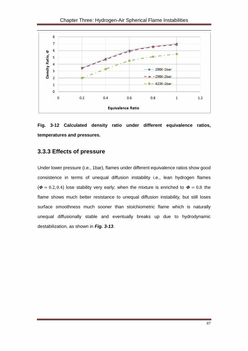
Chapter Three: Hydrogen-Air Spherical Flame Instabilities
87
Fig. 3-12 Calculated density ratio under different equivalence ratios,
temperatures and pressures.
3.3.3 Effects of pressure
Under lower pressure (i.e., 1bar), flames under different equivalence ratios show good
consistence in terms of unequal diffusion instability i.e., lean hydrogen flames
(𝜱 = 0.2, 0.4) lose stability very early; when the mixture is enriched to 𝜱 = 0.8 the
flame shows much better resistance to unequal diffusion instability, but still loses
surface smoothness much sooner than stoichiometric flame which is naturally
unequal diffusionally stable and eventually breaks up due to hydrodynamic
destabilization, as shown in Fig. 3-13.
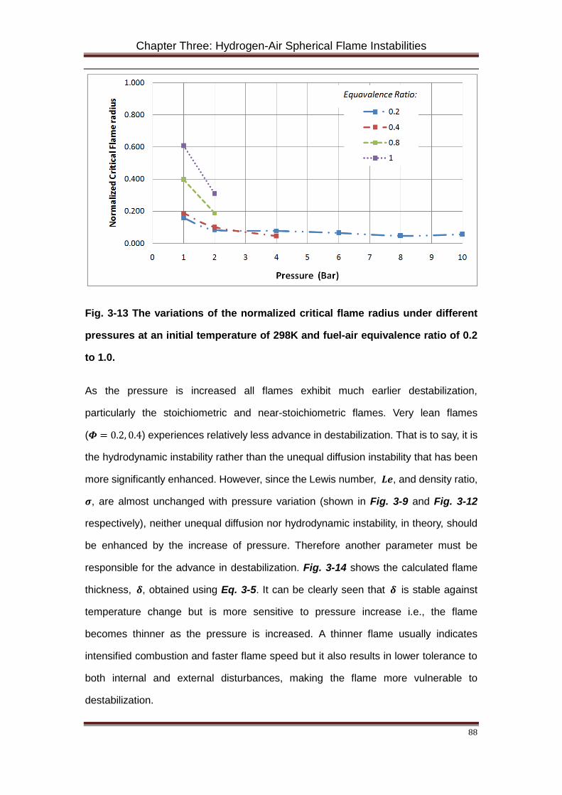
Chapter Three: Hydrogen-Air Spherical Flame Instabilities
88
Fig. 3-13 The variations of the normalized critical flame radius under different
pressures at an initial temperature of 298K and fuel-air equivalence ratio of 0.2
to 1.0.
As the pressure is increased all flames exhibit much earlier destabilization,
particularly the stoichiometric and near-stoichiometric flames. Very lean flames
(𝜱 = 0.2, 0.4) experiences relatively less advance in destabilization. That is to say, it is
the hydrodynamic instability rather than the unequal diffusion instability that has been
more significantly enhanced. However, since the Lewis number, 𝑳𝑳, and density ratio,
𝝈, are almost unchanged with pressure variation (shown in Fig. 3-9 and Fig. 3-12
respectively), neither unequal diffusion nor hydrodynamic instability, in theory, should
be enhanced by the increase of pressure. Therefore another parameter must be
responsible for the advance in destabilization. Fig. 3-14 shows the calculated flame
thickness, 𝜹, obtained using Eq. 3-5. It can be clearly seen that 𝜹 is stable against
temperature change but is more sensitive to pressure increase i.e., the flame
becomes thinner as the pressure is increased. A thinner flame usually indicates
intensified combustion and faster flame speed but it also results in lower tolerance to
both internal and external disturbances, making the flame more vulnerable to
destabilization.
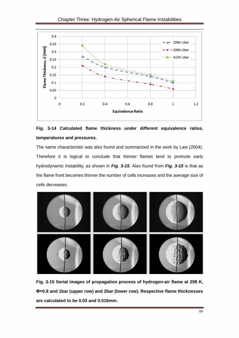
Chapter Three: Hydrogen-Air Spherical Flame Instabilities
89
Fig. 3-14 Calculated flame thickness under different equivalence ratios,
temperatures and pressures.
The same characteristic was also found and summarized in the work by Law (2004).
Therefore it is logical to conclude that thinner flames tend to promote early
hydrodynamic instability, as shown in Fig. 3-15. Also found from Fig. 3-15 is that as
the flame front becomes thinner the number of cells increases and the average size of
cells decreases.
Fig. 3-15 Serial images of propagation process of hydrogen-air flame at 298 K,
Φ=0.8 and 1bar (upper row) and 2bar (lower row). Respective flame thicknesses
are calculated to be 0.03 and 0.016mm.
Chapter Three: Hydrogen-Air Spherical Flame Instabilities
90
3.4 Summary
The onset of flame instabilities of laminar hydrogen-air spherical premixed flames has
been studied in a constant volume combustion bomb using high-speed Schlieren and
Shadow photography techniques. The effects of equivalence ratio, temperature and
pressure were identified and analysed. The following conclusions can be drawn
based on the analysis of experimental results:
• Outwardly propagating spherical flames experience two categories of instabilities:
unequal diffusion instability caused by unequal mass and thermal diffusion, and
hydrodynamic instability caused by interactions between the flame and external
disturbances.
• Unequal diffusion instability can be visually identified by the gradual growth and
branching of large cracks. Its appearance is governed by the Lewis number.
Stoichiometric hydrogen flames are naturally stable to unequal diffusion instability.
• Hydrodynamic instability can be visually identified by sudden and spontaneous
appearance of small cells across the entire flame surface. Changes to certain
parameters can only delay its appearance but not totally eliminate it.
• The onset of flame instabilities is identified by the means of measuring critical
flame radius. The critical radius is proven to be under the influences of
equivalence ratio, temperature and pressure.
• Equivalence ratio governs the value of the Lewis number, 𝑳𝑳, and therefore
decides whether the flame is naturally stable or instable to unequal diffusion
instability. When 𝑳𝑳 < 1 , cells induced by unequal diffusion effect grow
instantaneously at the beginning of flame kernel formation.
• Increased temperature has a strong delaying effect on the appearance of unequal
diffusion cells, particularly for very lean flame. The reason could be enhanced
combustion rate and flame speed that allow less time for the cells to appear and
grow. For stoichiometric flames, temperature increase reduces the density ratio,
𝝈, and therefore weakens the hydrodynamic instability.
Chapter Three: Hydrogen-Air Spherical Flame Instabilities
91
• Experimental results revealed that pressure is the most dominant of the three
parameters under investigation in terms of the onset of flame instability. Although
pressure variation barely affects either 𝑳𝑳 or 𝝈 which means it doesn’t enhance
unequal diffusion and hydrodynamic instabilities, but it affects the flame in a more
direct manner: by changing the flame thickness. Increased pressure significantly
weakens the flame front making it more vulnerable to destabilization. Higher
pressure also induces a larger number of cells of smaller average size.
Chapter Four: Calculation of Transient Stretched Laminar Flame Speed
92
Chapter Four: Calculation of Transient Stretched Laminar Flame Speed
4.1 Introduction
The calculation of the laminar burning velocities is one of the fundamental components in
modelling a variety of combustion systems, such as internal combustion (IC) engines. Some
studies were conducted in constant volume combustion experiments and the laminar burning
velocity was express as function of bomb pressure history, 𝒖𝒍 = � 𝟏𝑭𝟏𝑷
� �𝒓𝒄𝑷� �𝒅𝑷
𝒅𝒅� (Iijima &
Takeno 1986). Others using semi-empirical equations in the form of: 𝒖𝒍 = 𝒖𝒍𝟎 �𝑻𝒖𝑻𝟎�𝒂�𝑷𝒖𝑷𝟎�𝒃,
where 𝒖𝒍𝟎 is the reference laminar burning velocity at known mixture strength, temperature
and pressure, 𝒂 and 𝒃 are dependents determined experimentally (Lewis & von Elbe 1934).
More recently, Dowdy (1991) and Rahim (2002) developed methods, either linear or non-
linear, for extrapolating expressions of the mass fraction burnt and the instantaneous flame
speed using bomb pressure history. The authors claimed that these models were reliable
when the flame size was relatively small and the bomb pressure increase is not significant.
This is due to the fact that the relationship between the mass fraction burnt and the bomb
pressure becomes non-linear as the flame size exceeds approximately 10% of the size of
the combustion bomb (Dowdy et al. 1991; Rahim et al. 2002). In order to make above-
mentioned calculations work, full sets of experimental data, i.e. the exponents 𝒂 and 𝒃 and
the bomb pressure history, is a prerequisite. The accuracy of a and b depends on the range
of the experiments conducted. Numerous experiments with small increments of temperature
and pressure have to be conducted in order to maintain high fidelity, making it an expensive
and time consuming process (Lewis & von Elbe 1934; Metghalchi & Keck 1982; Metghalchi
& Keck 1980). Furthermore, it is difficult to integrate combustion chemistry into such
calculations, when prediction of combustion products has become increasingly important in
IC engine simulations. Some commercial packages, such as the Chemkin Fort�́� (Anon 2013),
integrate three-dimensional fluid dynamics and chemical kinetics to study the flame
propagation and emission formation processes in IC engines. These packages are capable
of providing simulation results of high complexity and accuracy, but at the costs of
computational time at the magnitude of hours. It would be a necessity to have a cost-
Chapter Four: Calculation of Transient Stretched Laminar Flame Speed
93
effective one-dimensional laminar burning velocity model that is integrated with combustion
chemistry.
The aim of this study is to develop a one-dimensional transient laminar burning velocity
model that eliminates the need for priori experiments and with the capability of solving
combustion chemistry. The model developed is based on a one-dimensional three-zone
thermodynamic model that calculates the mass transfer and diffusion and the heat transfer
between zones. The chemical processes involved in the combustion are solved using an in-
house chemical kinetics solver with an established reduced hydrogen-oxidation mechanism
from literature. The model has the potential to be adopted into future IC engine models for
the purpose of cost-effective combustion and emission formation studies.
4.2 Model Development
The propagation of a spherical flame front divides the combustion bomb into three distinctive
zones: burnt zone, burning zone and unburnt zone, as illustrated by Fig.4-1. The flame front
consumes the unburnt gas at the rate of the stretched laminar flame speed i.e. 𝑺𝒇 = 𝒅𝒓𝒇 𝒅𝒅⁄ ,
which can be seen as the result of the combination of three factors: the laminar burning
velocity, the relative thermal expansion and the flame stretch effects. The model
development starts with calculation of the laminar burning velocity and the effects of relative
thermal expansion and flame stretch will be added later.
The mode has a layered structure where the unburnt zone is divided into a number of thin
sub-layers, which is denoted by 𝒏 . The flame propagation process is seen as the
consecutive consumption of these thin unburnt layers. After the ignition, the flame will first
consume the innermost layer and this unburnt layer has become the burning zone. During
the consumption, the temperature and pressure will increase in the burning zone, thereby
compressing and heating up the rest of the unburnt zone. After a short period of time,
△ 𝒅𝒇𝒍𝒂𝒇𝒇, the consumption of the current burning layer completes and the flame then moves
into the adjacent unburnt layer (the second innermost one). The laminar burning velocity at
the nth layer is calculated as:
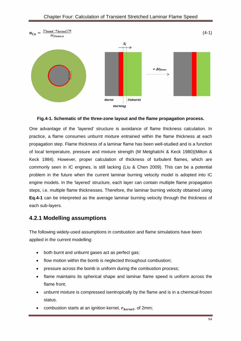
Chapter Four: Calculation of Transient Stretched Laminar Flame Speed
94
𝒖𝒍,𝒏 = (𝒓𝒃𝒃𝒇𝒃−𝒓𝒌𝒇𝒓𝒏𝒇𝒍)/𝒏∆𝒅𝒇𝒍𝒂𝒇𝒇,𝒏
(4-1)
Fig.4-1. Schematic of the three-zone layout and the flame propagation process.
One advantage of the ‘layered’ structure is avoidance of flame thickness calculation. In
practice, a flame consumes unburnt mixture entrained within the flame thickness at each
propagation step. Flame thickness of a laminar flame has been well-studied and is a function
of local temperature, pressure and mixture strength (M Metghalchi & Keck 1980)(Milton &
Keck 1984). However, proper calculation of thickness of turbulent flames, which are
commonly seen in IC engines, is still lacking (Liu & Chen 2009). This can be a potential
problem in the future when the current laminar burning velocity model is adopted into IC
engine models. In the ‘layered’ structure, each layer can contain multiple flame propagation
steps, i.e. multiple flame thicknesses. Therefore, the laminar burning velocity obtained using
Eq.4-1 can be interpreted as the average laminar burning velocity through the thickness of
each sub-layers.
4.2.1 Modelling assumptions
The following widely-used assumptions in combustion and flame simulations have been
applied in the current modelling:
• both burnt and unburnt gases act as perfect gas;
• flow motion within the bomb is neglected throughout combustion;
• pressure across the bomb is uniform during the combustion process;
• flame maintains its spherical shape and laminar flame speed is uniform across the
flame front;
• unburnt mixture is compressed isentropically by the flame and is in a chemical-frozen
status.
• combustion starts at an ignition kernel, 𝒓𝒌𝒇𝒓𝒏𝒇𝒍, of 2mm;
Chapter Four: Calculation of Transient Stretched Laminar Flame Speed
95
4.2.2 Governing equations
The unstretched laminar burning velocity is a fundamental combustion parameter and
depends only on temperature, pressure and equivalence ratio. Thus it is possible to
calculate the unstretched laminar burning velocity with thermodynamics and chemical
kinetics models. The thermodynamics model calculates the unburnt temperature, pressure
and mixture composition at each flame position as the flame propagates, and the chemical
kinetics model solves the combustion chemistry.
The principles of energy and mass conservation are applied to all three zones to describe
the energy flow within the combustion bomb.
Unburnt Zone: Temperature and pressure of the unburnt zone are influenced by two major
factors: the heat transfer from the flame and the compression work exerted by the flame.
These are described in Eq.4-2:
�𝒇𝒖 −𝒇𝒇� ∙ 𝑪𝒑,𝒖 ∙𝒅𝑻𝒖𝒅𝒅
= 𝑸𝒇,𝒖̇ + 𝑾𝒇̇ + 𝑸𝒇,𝒅̇ − 𝒇𝒇 ∙ 𝑯𝒖 (4-2)
where 𝒇𝒇 represents the mass entrained by the burning zone, 𝑸𝒇,𝒖̇ represents the
convective heat transfer from the flame to the unburnt zone and 𝑾𝒇̇ is the compression work
done by the volume change. 𝑯𝒖 represents the mean specific enthalpy of burning mixture at
𝑻𝒖.
𝑸𝒇,𝒖̇ = 𝒉𝒇 ∙ 𝑨𝒇 ∙ (𝑻𝒇 − 𝑻𝒖) (4-3)
𝑾𝒇̇ = 𝐏𝒖 ∙𝒅𝐕𝐮𝒅𝒅
(4-4)
where 𝒉𝒇 is the heat transfer coefficient, 𝑨𝒇 is the surface area of the flame, 𝑻𝒇 and 𝑻𝒖 are
the temperature of the flame and the unburnt zone respectively, 𝑽𝒖 represents the
instantaneous volume of the unburnt zone and 𝑷𝒖 is the unburnt pressure.
The heat transfer coefficient, 𝒉𝒇, for flame propagation inside internal combustion engines is
estimated as (Liu & Chen 2009):
𝒉𝒇 = 𝑪𝒉 ∙ 𝑩−𝟎.𝟐 ∙ 𝑷𝟎.𝟖 ∙ 𝒘𝟎.𝟖 ∙ 𝑻𝒇𝟎.𝟓𝟓 (4-5)
where 𝑪𝒉 is the heat transfer rate constant, 𝑩 is cylinder diameter, 𝒘 is the characteristic
speed within the cylinder. The term 𝑩 will be set as the diameter of the bomb, instead of that
of an engine cylinder.
Chapter Four: Calculation of Transient Stretched Laminar Flame Speed
96
Burnt Zone: All burnt mixtures are assumed to be in chemical equilibrium state (Daneshyar
& Hill 1987). The energy conservation of the burnt zone is in a similar manner to that of the
unburnt zone, except that the energy addition by mass transfer from the previous calculation
step has to be taken into account:
(𝒇𝒃 + 𝒇𝒇) ∙ 𝑪𝒑,𝒃 ∙𝒅𝑻𝒃𝒅𝒅
= 𝑸𝒇,𝒃̇ + 𝑽𝒃 ∙𝒅𝑷𝒅𝒅
+ 𝒇𝒇 ∙ 𝑯𝒇 (4-6)
where 𝒇𝒇 represents the burnt mass transferred from the burning zone into the burnt zone.
𝑯𝒇 represents the mean specific enthalpy of burning mixture at 𝑻𝒇.
Burning Zone: The energy flow within the burning zone is described by Eq. 7.
𝒇𝒇 ∙ 𝑪𝒑,𝒇 ∙𝒅𝑻𝒇𝒅𝒅
= 𝑸𝒄𝒉𝒇𝒇̇ + 𝑸𝒇,𝒖̇ + 𝑸𝒇,𝒃̇ − 𝑸𝒇,𝒅̇ (4-7)
where 𝑸𝒄𝒉𝒇𝒇̇ represents the primary heat release from chemical reactions and the kinetic
equations that describe the reactions within this layer are formulated as an ODE set (Liang
et al. 2009):
𝑸𝒄𝒉𝒇𝒇̇ = −∑ 𝒅𝒀𝒌𝒅𝒅
𝑲𝒌=𝟏
(∆𝒉𝒇𝟎)𝒌
𝑾𝒌 (4-8)
𝒅𝒀𝒌𝒅𝒅
= 𝝎𝒌̇𝝆𝑾𝒌 𝒌 = 𝟏, … ,𝑲 (4-9)
where (∆𝒉𝒇𝟎)𝒌 is the enthalpy of formation of the kth species, 𝝆 represents the density of the
reacting mixture, 𝝎𝒌̇ and 𝑾𝒌 are the molar production rate and molecular weight of the
species, respectively. In previous work (Saeed & Stone 2004; Byun 2011), the heat transfer
from the flame front to the bomb walls has been found to be negligible and is therefore not
included in the model.
The term 𝑸𝒇,𝒅̇ takes into account of the energy transfer due to the diffusion effect of burning
mixtures to the unburnt zone. It is evaluated using the mixture-averaged method introduced
in the TRANSPORT library in the CHEMKIN-III package (Kee et al. 1996):
𝑸𝒇,𝒅̇ = 𝑯𝒇
𝒄𝒑∑ 𝝆 ∙𝑲𝒌=𝟏
𝒅𝒀𝒌𝒅𝒅
∙ 𝑽𝒌 ∙ 𝒄𝒑,𝒌 (4-10)
where 𝑽𝒌and 𝒄𝒑,𝒌 are, respectively, the diffusion velocity and constant pressure and the heat
capacity of the kth species.
Chapter Four: Calculation of Transient Stretched Laminar Flame Speed
97
4.2.3 Chemical kinetics mechanism
The accuracy of unstretched laminar burning velocity calculation depends on the realism of
the kinetics mechanism and the accuracy of the reaction rates. Hydrogen combustion
kinetics has been widely studied (Mueller et al. 1999)(Vlachos 1996)(Law et al. 2003)(O
Conaire et al. 2004)(Li et al. 2004)(Konnov 2008)(Hu et al. 2009). The hydrogen combustion
kinetics mechanism used in the current research is the mechanism consists of 11 species
and 19 reversible elementary reactions (Burke et al. 2011). The major improvements of this
mechanism over previous mechanism include: clarification of uncertainties in the
temperature and pressure dependence of rate constants for HO2 formation/consumption
reactions; demonstration of the pressure dependence of H+O2=OH+O and the temperature
dependence of the H+HO2 channels. The thermo-chemical data for the species involved are
computed using the CHEMKIN-III package. An in-house chemical kinetics solver (Liu & Chen
2009) will be used in the burning zone to calculate the reaction rates of each elementary
reaction and concentration variations of each reactants.
4.2.4 Defining of the end of in-flame reactions
In order to calculate the in-flame reaction duration, △ 𝒅𝒇𝒍𝒂𝒇𝒇 , needed in Eq.4-1, one
parameter that defines the end of the in-flame reaction need to be defined. The end of the in-
flame reactions is not necessarily the end of the overall reactions occurs between the fuel
and oxidant entrained into the flame. Together with intermediate products, a tiny amount of
unburnt fuel and oxidant will continue reacting after being transferred into the burnt zone,
this is commonly known as post-flame reactions .
In-flame reactions are characterized as high reaction rate and rapid energy release while
post-flame reactions are relatively slow and release less energy. Therefore, reaction rates of
some active intermediate products would be a sensible indication of the transit from in-flame
to post-flame reactions. The H radical is known to be a very important intermediate product
in hydrogen and hydrocarbon oxidations (Li et al. 2004)(Burke et al. 2011). It provides critical
channels for H+O2 and H+HO2 reactions. As shown in Fig.4-2, the change in the
concentration of the H radical is closely related to consumptions of fuel and oxidant and the
temperature increase (energy release). Fig.4-3 shows the variations of H radical mole
fraction and its change rate, 𝒀�̇�.
𝒀�̇� = (𝒀𝑯 − 𝒀𝑯′ )/∆𝐭 (4-11)
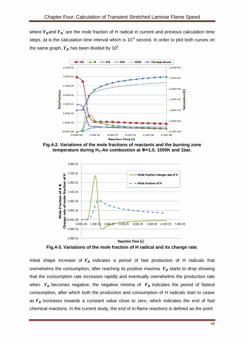
Chapter Four: Calculation of Transient Stretched Laminar Flame Speed
98
where 𝒀𝑯and 𝒀𝑯′ are the mole fraction of H radical in current and previous calculation time
steps. ∆𝐭 is the calculation time interval which is 10-6 second. In order to plot both curves on
the same graph, 𝒀�̇� has been divided by 105.
Fig.4-2. Variations of the mole fractions of reactants and the burning zone temperature during H2-Air combustion at Ф=1.0, 1000K and 1bar.
Fig.4-3. Variations of the mole fraction of H radical and its change rate.
Initial shape increase of 𝒀�̇� indicates a period of fast production of H radicals that
overwhelms the consumption; after reaching its positive maxima 𝒀�̇� starts to drop showing
that the consumption rate increases rapidly and eventually overwhelms the production rate
when 𝒀�̇� becomes negative; the negative minima of 𝒀�̇� indicates the period of fastest
consumption, after which both the production and consumption of H radicals start to cease
as 𝒀�̇� increases towards a constant value close to zero, which indicates the end of fast
chemical reactions. In the current study, the end of in-flame reactions is defined as the point
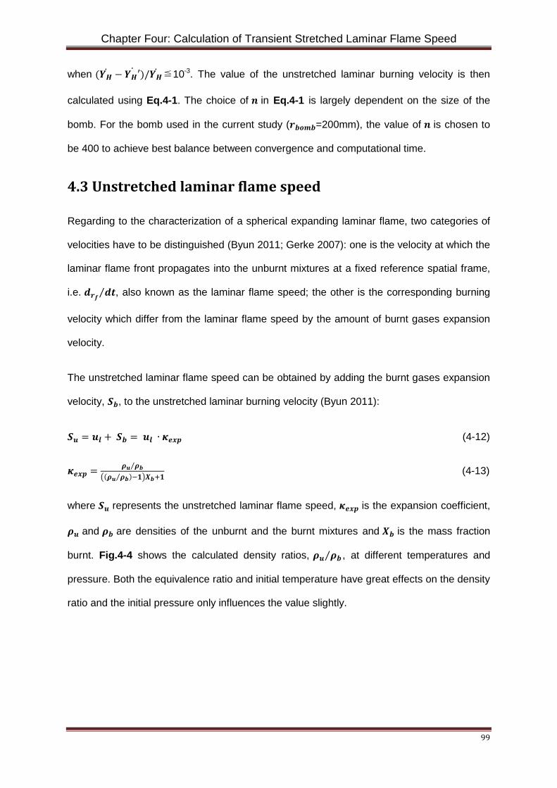
Chapter Four: Calculation of Transient Stretched Laminar Flame Speed
99
when (𝒀�̇� − 𝒀𝑯′̇ )/𝒀�̇�≦10-3. The value of the unstretched laminar burning velocity is then
calculated using Eq.4-1. The choice of 𝒏 in Eq.4-1 is largely dependent on the size of the
bomb. For the bomb used in the current study (𝒓𝒃𝒃𝒇𝒃=200mm), the value of 𝒏 is chosen to
be 400 to achieve best balance between convergence and computational time.
4.3 Unstretched laminar flame speed
Regarding to the characterization of a spherical expanding laminar flame, two categories of
velocities have to be distinguished (Byun 2011; Gerke 2007): one is the velocity at which the
laminar flame front propagates into the unburnt mixtures at a fixed reference spatial frame,
i.e. 𝒅𝒓𝒇 𝒅𝒅⁄ , also known as the laminar flame speed; the other is the corresponding burning
velocity which differ from the laminar flame speed by the amount of burnt gases expansion
velocity.
The unstretched laminar flame speed can be obtained by adding the burnt gases expansion
velocity, 𝑺𝒃, to the unstretched laminar burning velocity (Byun 2011):
𝑺𝒖 = 𝒖𝒍 + 𝑺𝒃 = 𝒖𝒍 ∙ 𝜿𝒇𝒆𝒑 (4-12)
𝜿𝒇𝒆𝒑 = 𝝆𝒖 𝝆𝒃⁄�(𝝆𝒖 𝝆𝒃⁄ )−𝟏�𝑿𝒃+𝟏
(4-13)
where 𝑺𝒖 represents the unstretched laminar flame speed, 𝜿𝒇𝒆𝒑 is the expansion coefficient,
𝝆𝒖 and 𝝆𝒃 are densities of the unburnt and the burnt mixtures and 𝑿𝒃 is the mass fraction
burnt. Fig.4-4 shows the calculated density ratios, 𝝆𝒖 𝝆𝒃⁄ , at different temperatures and
pressure. Both the equivalence ratio and initial temperature have great effects on the density
ratio and the initial pressure only influences the value slightly.
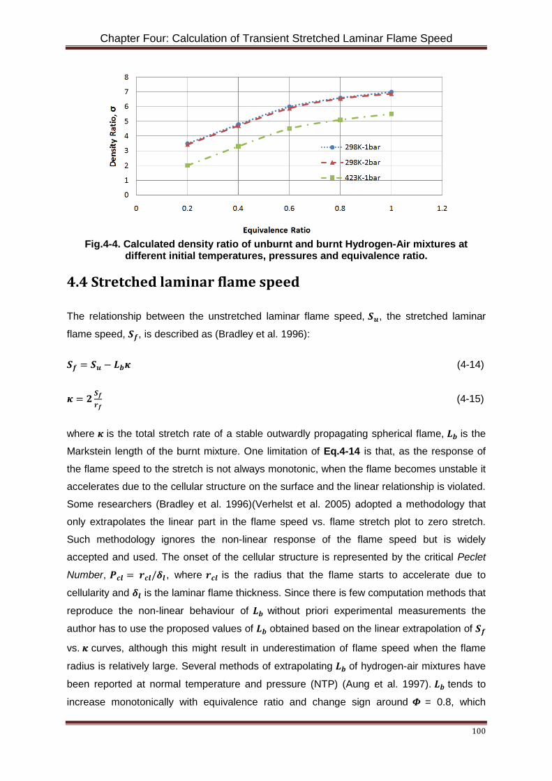
Chapter Four: Calculation of Transient Stretched Laminar Flame Speed
100
Fig.4-4. Calculated density ratio of unburnt and burnt Hydrogen-Air mixtures at different initial temperatures, pressures and equivalence ratio.
4.4 Stretched laminar flame speed
The relationship between the unstretched laminar flame speed, 𝑺𝒖, the stretched laminar
flame speed, 𝑺𝒇, is described as (Bradley et al. 1996):
𝑺𝒇 = 𝑺𝒖 − 𝑳𝒃𝜿 (4-14)
𝜿 = 𝟐 𝑺𝒇𝒓𝒇
(4-15)
where 𝜿 is the total stretch rate of a stable outwardly propagating spherical flame, 𝑳𝒃 is the
Markstein length of the burnt mixture. One limitation of Eq.4-14 is that, as the response of
the flame speed to the stretch is not always monotonic, when the flame becomes unstable it
accelerates due to the cellular structure on the surface and the linear relationship is violated.
Some researchers (Bradley et al. 1996)(Verhelst et al. 2005) adopted a methodology that
only extrapolates the linear part in the flame speed vs. flame stretch plot to zero stretch.
Such methodology ignores the non-linear response of the flame speed but is widely
accepted and used. The onset of the cellular structure is represented by the critical Peclet
Number, 𝑷𝒄𝒍 = 𝒓𝒄𝒍/𝜹𝒍 , where 𝒓𝒄𝒍 is the radius that the flame starts to accelerate due to
cellularity and 𝜹𝒍 is the laminar flame thickness. Since there is few computation methods that
reproduce the non-linear behaviour of 𝑳𝒃 without priori experimental measurements the
author has to use the proposed values of 𝑳𝒃 obtained based on the linear extrapolation of 𝑺𝒇
vs. 𝜿 curves, although this might result in underestimation of flame speed when the flame
radius is relatively large. Several methods of extrapolating 𝑳𝒃 of hydrogen-air mixtures have
been reported at normal temperature and pressure (NTP) (Aung et al. 1997). 𝑳𝒃 tends to
increase monotonically with equivalence ratio and change sign around 𝜱 = 0.8, which
Chapter Four: Calculation of Transient Stretched Laminar Flame Speed
101
implies that lean mixtures experience an earlier transition to unstable cellular structure.
Verhelst (Verhelst et al. 2005) proposed values of 𝑳𝒃 for higher temperature and pressure by
using the regression methodology developed by Bradley (Bradley et al. 1996). These values
will be used in the current study.
Finally, based on Eq. 1and 12-15 and the relationship between stretched and unstretched
laminar flame speed, 𝑺𝒇 can be obtained as:
𝑺𝒇 = 𝒖𝒍 ∙ 𝝆𝒖 𝝆𝒃⁄�(𝝆𝒖 𝝆𝒃⁄ )−𝟏�𝑿𝒃+𝟏
− 𝑳𝒃𝟐∙𝑺𝒇𝒓𝒇
(4-16)
In the RHS of Eq.4-16, the stretched laminar flame speed is represented as a combination of
the unstretched laminar burning velocity, the relative thermal expansion, and the flame
stretch effect.
4.5. Model Validation
4.5.1 Experimental apparatus
A spherical stainless steel combustion bomb with 400mm inner diameter which is capable of
withstanding the temperature and pressure generated by combustion with initial conditions
up to 1.5MPa and 650K, as shown in Fig.3-4 in Chapter Three, has been employed. The
bomb has extensive optical access through a pair of orthogonal quartz windows of 100mm
diameter. The optical system is arranged into a Z-shaped, the two primary mirrors have
diameter of 100mm and focal length of 100cm.The slit has an adjustment range of 0-3mm
and the blade can be adjusted in the range of 0-10mm. There are two intake routes, one for
air, and the other for hydrogen. Low-pressure sensor is used to accurately measure partial
pressure of gas with the precision of 0.001bar.The combustible mixture is spark ignited at
centre of the chamber using electrodes extending from the top and the bottom. One
electrode is fixed while the other could be moved for adjusting the ignition gap. After the
induction of fuel and air is completed sufficient time is allowed for the mixture motion to
decay. The bomb is flushed with dry air when combustion is finished to ensure minimum
amount of residuals are left before subsequent combustion is initiated. Following the ignition,
gas temperature inside the bomb is obtained from two chrome–alumel thermocouples.
Pressure is measured during the explosion with a Kistler pressure transducer. Flame images
are recorded by a TRI Phantom v7.3 camera which is capable of a maximum speed of
200,000 frames per second. Additional information on the experimental apparatus can be
found in literature (Liu et al. 2011).
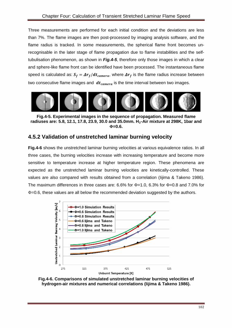
Chapter Four: Calculation of Transient Stretched Laminar Flame Speed
102
Three measurements are performed for each initial condition and the deviations are less
than 7%. The flame images are then post-processed by imaging analysis software, and the
flame radius is tracked. In some measurements, the spherical flame front becomes un-
recognisable in the later stage of flame propagation due to flame instabilities and the self-
tubulisation phenomenon, as shown in Fig.4-5, therefore only those images in which a clear
and sphere-like flame front can be identified have been processed. The instantaneous flame
speed is calculated as: 𝑺𝒇 = 𝜟𝒓𝒇/𝒅𝒅𝒄𝒂𝒇𝒇𝒓𝒂, where 𝜟𝒓𝒇 is the flame radius increase between
two consecutive flame images and 𝒅𝒅𝒄𝒂𝒇𝒇𝒓𝒂 is the time interval between two images.
Fig.4-5. Experimental images in the sequence of propagation. Measured flame radiuses are: 5.8, 12.1, 17.8, 23.9, 30.0 and 35.0mm. H2-Air mixture at 298K, 1bar and
Φ=0.6.
4.5.2 Validation of unstretched laminar burning velocity
Fig.4-6 shows the unstretched laminar burning velocities at various equivalence ratios. In all
three cases, the burning velocities increase with increasing temperature and become more
sensitive to temperature increase at higher temperature region. These phenomena are
expected as the unstretched laminar burning velocities are kinetically-controlled. These
values are also compared with results obtained from a correlation (Iijima & Takeno 1986).
The maximum differences in three cases are: 6.6% for Ф=1.0, 6.3% for Ф=0.8 and 7.0% for
Ф=0.6, these values are all below the recommended deviation suggested by the authors.
Fig.4-6. Comparisons of simulated unstretched laminar burning velocities of hydrogen-air mixtures and numerical correlations (Iijima & Takeno 1986).
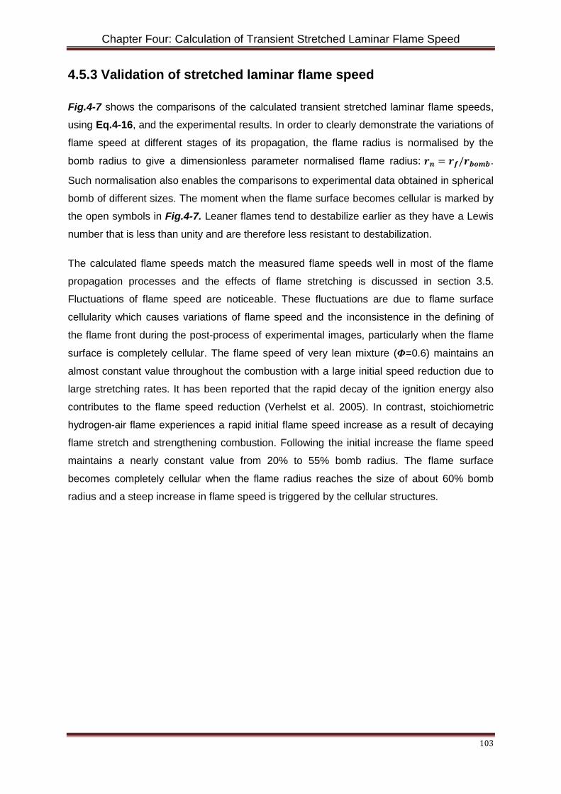
Chapter Four: Calculation of Transient Stretched Laminar Flame Speed
103
4.5.3 Validation of stretched laminar flame speed
Fig.4-7 shows the comparisons of the calculated transient stretched laminar flame speeds,
using Eq.4-16, and the experimental results. In order to clearly demonstrate the variations of
flame speed at different stages of its propagation, the flame radius is normalised by the
bomb radius to give a dimensionless parameter normalised flame radius: 𝒓𝒏 = 𝒓𝒇/𝒓𝒃𝒃𝒇𝒃.
Such normalisation also enables the comparisons to experimental data obtained in spherical
bomb of different sizes. The moment when the flame surface becomes cellular is marked by
the open symbols in Fig.4-7. Leaner flames tend to destabilize earlier as they have a Lewis
number that is less than unity and are therefore less resistant to destabilization.
The calculated flame speeds match the measured flame speeds well in most of the flame
propagation processes and the effects of flame stretching is discussed in section 3.5.
Fluctuations of flame speed are noticeable. These fluctuations are due to flame surface
cellularity which causes variations of flame speed and the inconsistence in the defining of
the flame front during the post-process of experimental images, particularly when the flame
surface is completely cellular. The flame speed of very lean mixture (𝜱=0.6) maintains an
almost constant value throughout the combustion with a large initial speed reduction due to
large stretching rates. It has been reported that the rapid decay of the ignition energy also
contributes to the flame speed reduction (Verhelst et al. 2005). In contrast, stoichiometric
hydrogen-air flame experiences a rapid initial flame speed increase as a result of decaying
flame stretch and strengthening combustion. Following the initial increase the flame speed
maintains a nearly constant value from 20% to 55% bomb radius. The flame surface
becomes completely cellular when the flame radius reaches the size of about 60% bomb
radius and a steep increase in flame speed is triggered by the cellular structures.
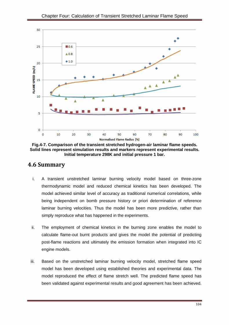
Chapter Four: Calculation of Transient Stretched Laminar Flame Speed
104
Fig.4-7. Comparison of the transient stretched hydrogen-air laminar flame speeds. Solid lines represent simulation results and markers represent experimental results.
Initial temperature 298K and initial pressure 1 bar.
4.6 Summary
i. A transient unstretched laminar burning velocity model based on three-zone
thermodynamic model and reduced chemical kinetics has been developed. The
model achieved similar level of accuracy as traditional numerical correlations, while
being independent on bomb pressure history or priori determination of reference
laminar burning velocities. Thus the model has been more predictive, rather than
simply reproduce what has happened in the experiments.
ii. The employment of chemical kinetics in the burning zone enables the model to
calculate flame-out burnt products and gives the model the potential of predicting
post-flame reactions and ultimately the emission formation when integrated into IC
engine models.
iii. Based on the unstretched laminar burning velocity model, stretched flame speed
model has been developed using established theories and experimental data. The
model reproduced the effect of flame stretch well. The predicted flame speed has
been validated against experimental results and good agreement has been achieved.
Chapter Four: Calculation of Transient Stretched Laminar Flame Speed
105
Flame speed has been found to increase with increased fuel-air equivalence ratio
(from 0.6 to 1.0), temperature and pressure.
iv. The timing of the end of in-flame reactions has not been thoroughly studied and
clearly defined in the literature. The choice of using the change rate of the
concentration of H radical to define the end of the in-flame reactions is based on the
literature study of hydrogen oxidation mechanisms, where the H radical has been
identified as one of the most active intermediate products and is directly related to
the consumptions of the fuel and the energy release rate.
v. Since a method that predicts the non-linear behaviour of Markstein length,
particularly after the flame surface is cellular, is not yet available, the authors have to
adopt the linear Markstein length, this results in underestimation of laminar flame
speed when the flame front is cellular. Future improvement of the model should be
focused in this area.
vi. The developed model requires less computational power and completes calculation
for flame speeds in a combustion bomb of 200mm inner radius in the magnitude of
fifteen seconds. The computational costs are expected to be in the magnitude of a
few minutes when the developed model is integrated into IC engine simulations,
which represents a noticeable saving on computational costs.
Chapter Five: SI Engine Flame Propagation Simulation
106
Chapter Five: Simulation of Flame
Propagation in SI Engine
5.1 Introduction
Turbulent flame propagation within the combustion chamber is inherently unsteady
(Heywood 1988) and is of great importance to spark ignition engine operation. Firstly,
the unburnt charge, theoretically, is to be consumed by the propagating flame front in
a sequential manner, therefore, the flame is responsible for combustion efficiency and
cycle-to-cycle variations; Secondly, the propagating flame front is widely accepted as
one of the major factors that contributes to the end gas autoignition. The key
parameter for systematic understand of accurate prediction of combustion process is
knowledge of the burning rate of the flame propagating through the charge (Liu et al.
2013). Due to the unsteady and transient nature of turbulent flames, extrapolation of
experimental results obtain in laboratory conditions, i.e. NTP, is very difficult because
of high in-cylinder temperature and pressure (Liu et al. 2013; Aleiferis & Rosati 2012;
Peterson et al. 2014; Dahms et al. 2011).
In recent decades, numerical engine combustion simulation is becoming a powerful
and cost-effective (when compared to engine testing) tool in the research and design
of spark ignition engines. There are different levels of spark ignition engine
combustion models. Computation fluid dynamics (CFD) modelling coupled with
detailed (Long & Reitz n.d.), reduced (Blunsdon & Dent 1994; Eckert et al. 2003; Kong
et al. 1995) and global (Liu et al. 2006) chemical kinetics showed a potential of
replicate the turbulent flame propagation and predict abnormal combustion
Chapter Five: SI Engine Flame Propagation Simulation
107
phenomenon, e.g. knock, in spark ignition engines. The chemical kinetics mechanism
is applied to account for the temporal and spatial variance of the properties of unburnt
mixture. The actual turbulent flame speed is calculated using a turbulent flame speed
closure and an empirical correlation of laminar flame speed (Zimont & Polifke 1998).
The combination of CFD thermodynamics model and chemical kinetics model
provides sufficient accuracy but it comes with massive computational costs.
Additionally, because empirical laminar flame speed correlations are fuel specific and
only reliable in a limited range of operating conditions, the flexibility of the model is
affected. Simpler spark ignition models have been developed using zero-dimensional
modelling technique. These models use chemical equilibrium combustion models to
determine the thermo-chemical state of the burnt products at a predefined flame
temperature. These models are computationally efficient, and provide a handy tool in
engine design and operating strategy testing. However, the turbulent flame
propagation process is completely neglected and replace by a function of burnt mass
fraction, i.e. Wiebe function (Shayler et al. 1990; Stone 1987; Rakopoulos & Michos
2008; Shudo et al. 2001; Ball et al. 1998; Rousseau et al. 1999; Ghojel 2010). The
use of chemical equilibrium makes these models functionally unable to predict end
gas autoignition. Liu (Liu & Chen 2009) greatly improved models of this kind by having
a three-zone formation and adopting a reduced gasoline chemical kinetics
mechanism into the unburnt zone to not only the combustion but also the onset of
knock. Liu’s work has broadened the usage of models based on zero-dimensional
thermodynamics and chemical kinetics for spark ignition engine research.
The current research has been vastly motivated by Liu’s work. The purpose of current
research is to implement the developed chemical kinetic laminar flame speed model
(introduced in chapter four), together with an ‘out-of-box’ turbulent flame speed
correlation, into a zero-dimensional multi-zone thermodynamics model to simulate the
turbulent flame propagation process within the combustion chamber.
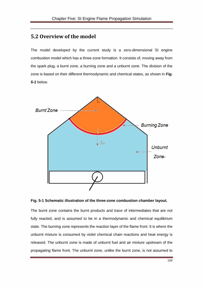
Chapter Five: SI Engine Flame Propagation Simulation
108
5.2 Overview of the model
The model developed by the current study is a zero-dimensional SI engine
combustion model which has a three-zone formation. It consists of, moving away from
the spark plug, a burnt zone, a burning zone and a unburnt zone. The division of the
zone is based on their different thermodynamic and chemical states, as shown in Fig.
5-1 below.
Fig. 5-1 Schematic illustration of the three-zone combustion chamber layout.
The burnt zone contains the burnt products and trace of intermediates that are not
fully reacted, and is assumed to be in a thermodynamic and chemical equilibrium
state. The burning zone represents the reaction layer of the flame front. It is where the
unburnt mixture is consumed by violet chemical chain reactions and heat energy is
released. The unburnt zone is made of unburnt fuel and air mixture upstream of the
propagating flame front. The unburnt zone, unlike the burnt zone, is not assumed to
Chapter Five: SI Engine Flame Propagation Simulation
109
be in a thermodynamic and chemical equilibrium state. The temperature and pressure
in this zone is allowed to vary as a result of piston motion, flame propagation and heat
transfer.
A modified version of Tanaka’s chemical kinetics mechanism (Tanaka et al. 2003) is
applied to both the burning and the unburnt zone in order to:
Study the combustion process within the flame front by calculating a number
of parameters including: flame temperature, species concentration evolution
and combustion duration.
Predict autoignition of unburnt mixture and onset timing of knock.
The modification was carried out by Liu et al. (2009) in order to adapt the mechanism
into spark ignition engine combustion simulation, as the original mechanism was
developed for HCCI combustion.
The simulation model consists of five major components:
A engine cylinder model
A flame geometry model
A zero-dimensional thermodynamics model
An in-cylinder turbulence model
A chemical kinetics model (applied in two zones)
These components will be introduced in the following sections.
5.2.1 Model assumptions
The proposed model is a mathematical model of the compression and combustion
(BDC-TDC-BDC) processes in a premixed naturally aspirated spark ignition engine.
Some assumptions are applied in the development of the model:
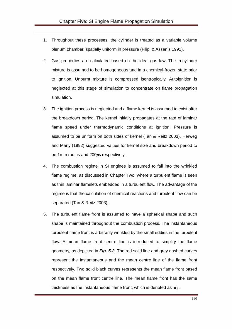
Chapter Five: SI Engine Flame Propagation Simulation
110
1. Throughout these processes, the cylinder is treated as a variable volume
plenum chamber, spatially uniform in pressure (Filipi & Assanis 1991).
2. Gas properties are calculated based on the ideal gas law. The in-cylinder
mixture is assumed to be homogeneous and in a chemical-frozen state prior
to ignition. Unburnt mixture is compressed isentropically. Autoignition is
neglected at this stage of simulation to concentrate on flame propagation
simulation.
3. The ignition process is neglected and a flame kernel is assumed to exist after
the breakdown period. The kernel initially propagates at the rate of laminar
flame speed under thermodynamic conditions at ignition. Pressure is
assumed to be uniform on both sides of kernel (Tan & Reitz 2003). Herweg
and Marly (1992) suggested values for kernel size and breakdown period to
be 1mm radius and 200μs respectively.
4. The combustion regime in SI engines is assumed to fall into the wrinkled
flame regime, as discussed in Chapter Two, where a turbulent flame is seen
as thin laminar flamelets embedded in a turbulent flow. The advantage of the
regime is that the calculation of chemical reactions and turbulent flow can be
separated (Tan & Reitz 2003).
5. The turbulent flame front is assumed to have a spherical shape and such
shape is maintained throughout the combustion process. The instantaneous
turbulent flame front is arbitrarily wrinkled by the small eddies in the turbulent
flow. A mean flame front centre line is introduced to simplify the flame
geometry, as depicted in Fig. 5-2. The red solid line and grey dashed curves
represent the instantaneous and the mean centre line of the flame front
respectively. Two solid black curves represents the mean flame front based
on the mean flame front centre line. The mean flame front has the same
thickness as the instantaneous flame front, which is denoted as 𝜹𝑻.
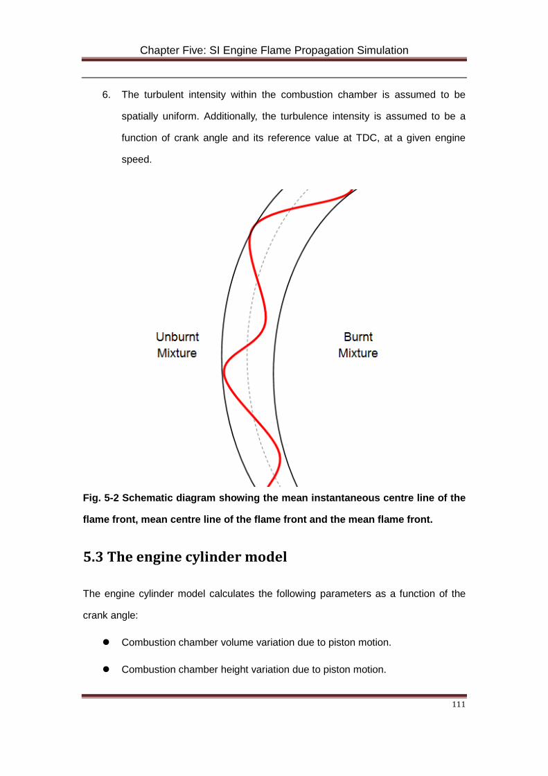
Chapter Five: SI Engine Flame Propagation Simulation
111
6. The turbulent intensity within the combustion chamber is assumed to be
spatially uniform. Additionally, the turbulence intensity is assumed to be a
function of crank angle and its reference value at TDC, at a given engine
speed.
Fig. 5-2 Schematic diagram showing the mean instantaneous centre line of the
flame front, mean centre line of the flame front and the mean flame front.
5.3 The engine cylinder model
The engine cylinder model calculates the following parameters as a function of the
crank angle:
Combustion chamber volume variation due to piston motion.
Combustion chamber height variation due to piston motion.
Chapter Five: SI Engine Flame Propagation Simulation
112
Cylinder area variation due to piston motion.
Unburnt mixture temperature and pressure variations due to piston motion
and convective heat transfer from/to the walls.
5.3.1 In-cylinder volume derivation
The volume of the cylinder and its derivative are calculated as a function of crank
angle from the compression ratio, stroke, bore and connecting rod length (Shaver &
Gerdes 2003).
Fig. 5-3 Illustration of a typical piston-crank-cylinder assembly.
In Fig. 5-3 b is cylinder bore, s is stroke of the engine, l is the connecting rod length
and a is the crank radius. The volume of the combustion chamber when piston is at
TDC is referred as the clearance volume, Vc, the volume when piston is at BDC is the
maximum volume of the cylinder, Vmax. the volume in between Vmax and Vc is known as
the displacement volume, Vd.
𝑽𝒅 = 𝝅𝟒∙ 𝒃𝟐 ∙ 𝒔 (5-1)
At a given crank angle, the instantaneous chamber volume is expressed as:
𝑽 = 𝝅𝟒∙ 𝒃𝟐 ∙ 𝑯 + 𝑽𝒄 (5-2)
Chapter Five: SI Engine Flame Propagation Simulation
113
where 𝑯 is the instantaneous chamber height:
𝑯 = 𝒂 + 𝒍 − [�𝒍𝟐 − 𝒂𝟐𝑺𝑺𝑺𝟐𝜽�𝟎.𝟓 + 𝒂𝒄𝒄𝒔𝜽] (5-3)
The compression ratio is defined as r =Vmax/ Vc and therefore r =1+Vd/ Vc. Solving for
Vc yields:
𝑽𝒄 = 𝑽𝒅𝒓−𝟏
(5-4)
Substituting Eq. 5-4 and 5-4 into Eq. 5-2:
𝑽 = 𝑽𝒅𝒓−𝟏
+ 𝑽𝒅𝟐
[𝟏 + 𝑹− 𝒄𝒄𝒔𝜽 − (𝑹𝟐 − 𝑺𝑺𝑺𝟐𝜽)𝟎.𝟓] (5-5)
The predicted instantaneous combustion chamber height and volume are shown in
Fig. 5-4.
5.3.2 Surface area derivation
In order to study the heat transfer between the flame and the cylinder walls, 𝑨𝑾,
cylinder head, 𝑨𝑯, and the piston head, 𝑨𝑷, the instantaneous surface area of the
cylinder, 𝑨, has been evaluated:
𝑨 = 𝑨𝑾 + 𝑨𝑯 + 𝑨𝑷 = 𝝅𝒃𝝅 + 𝟏𝟐 ∗ 𝑽𝒄𝒃
+ 𝝅𝟒∙ 𝒃𝟐 (5-6)
The predicted instantaneous cylinder area is shown in Fig.5-4
5.4 The flame geometry model
The flame is assumed to be initiated at the cone tip of the combustion chamber and
propagates downwards to the piston. Due to relative motion and positions of the flame
front and the piston, a number of possible flame front geometries may occur during its
propagation by comparing the cone radius, 𝑹𝒄𝒄𝑺𝒄 and the instantaneous chamber
height, H. The resultant flame geometries are illustrated in Fig. 5-5 and Table 5-1
below.
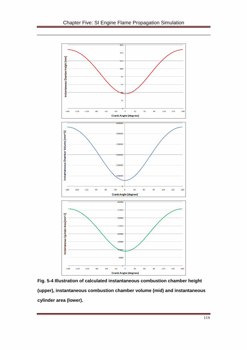
Chapter Five: SI Engine Flame Propagation Simulation
114
Fig. 5-4 Illustration of calculated instantaneous combustion chamber height
(upper), instantaneous combustion chamber volume (mid) and instantaneous
cylinder area (lower).
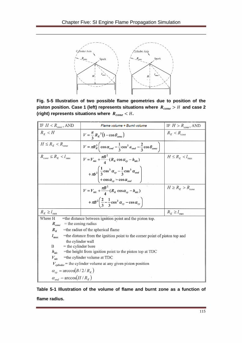
Chapter Five: SI Engine Flame Propagation Simulation
115
Fig. 5-5 Illustration of two possible flame geometries due to position of the piston position. Case 1 (left) represents situations where 𝑹𝒄𝒄𝑺𝒄 > 𝐻 and case 2 (right) represents situations where 𝑹𝒄𝒄𝑺𝒄 < 𝐻.
Table 5-1 Illustration of the volume of flame and burnt zone as a function of
flame radius.
Chapter Five: SI Engine Flame Propagation Simulation
116
5.5 The thermodynamics model
5.5.1 Volume of combustion chamber
The combustion chamber volume varies as a function of crank angle and as a result
of piston motion. Nevertheless, the instantaneous chamber volume at any given crank
angle is conserved:
𝑽 = 𝑽𝒃 + 𝑽𝒇 + 𝑽𝒖 (5-7)
where 𝑽𝒃, 𝑽𝒇, 𝑽𝒖 are volumes at the beginning of each calculation step.
5.5.2 Conservation of mass and species:
The total mass at the start of compression stroke (BDC) is conserved throughout
compression and combustion stroke:
𝒎 = 𝒎𝒃 + 𝒎𝒇 + 𝒎𝒖 (5-8)
where 𝒎𝒃, 𝒎𝒇, 𝒎𝒖 are mass at the beginning of each calculation step.
𝒎𝒖 = 𝒎𝒖′ −𝒎𝒇 (5-9)
𝒎𝒃 = 𝒎𝒃′ + 𝒎𝒇′ (5-10)
where 𝒎𝒖′, 𝒎𝒇′ and 𝒎𝒃′ are mass of the previous calculation step.
The species in three zones are also conserved. The concentrations of any species in
unburnt and burning zones are expressed as:
𝒅𝑿𝑺,𝒋𝒅𝒅
= 𝑴𝑺∙𝝎𝒊̇𝝆𝒋
(5-11)
where X represents the mass fraction of a species. Subscripts i and j denote the
species and zones considered. 𝑴𝑺 and 𝝎𝑺 represents the molecular weight and
molar production rate of species i respectively. Similar expression for the burnt zone
can also be obtained:
Chapter Five: SI Engine Flame Propagation Simulation
117
𝒅𝑿𝑺,𝒃𝒅𝒅
= 𝟏𝒎𝒃
𝒅𝒎𝒃𝒅𝒅
∙ �𝑿𝑺,𝒇 − 𝑿𝑺,𝒃�+ 𝑴𝑺∙𝝎𝑺̇𝝆𝒃
(5-12)
5.5.3 Conservation of energy
The energy conservation equations for burnt, burning and unburnt zone are described
in Section 4.2 in Chapter Four in details. The same set of equations is used here.
5.6 The chemical kinetics model
The chemical kinetics model used in the current research is a modified version of
Tanaka mechanism (Tanaka et al. 2003). The mechanism was originally developed for
mixtures of n-heptane and iso-octane in HCCI combustion mode and modified by Liu
(Liu & Chen 2009) to suit SI combustion simulation.
The modification process is briefly introduced below. Sensitivity analysis on the
Tanaka mechanism showed that R6 and R18 (generally expressed as RH + OH = R
+H2O) were the most influential on both the ignition delay and the burn rate. The
enhancement of their pre-exponential constants of the rate constants leads to a
shorter ignition delay and a higher burn-rate. This phenomenon is attributed to the
role of alkyl radical formation reactions in the oxidation chemistry, where both
reactions represent the attack of the active radical OH to abstract the atom H from fuel
molecules. The pre-exponential constants were enhanced by a factor of 1 to 10, and
the modified mechanism was put into the model to investigate its effect on knock
onset, knock intensity, combustion duration and peak cylinder pressure. The results
show that the increase of the enhance factors from 1 to 6 leads to knock position
being advanced by about 23%, the peak pressure being increased by around 16%,
and knock intensity being raised by about 100%. Further increasing the enhance
factors from 6.0 to 10.0 can only affect these three parameters by about 3%, 2%, and
15%, respectively. Thus, it was concluded the enhance factor of the value of 6.0 was
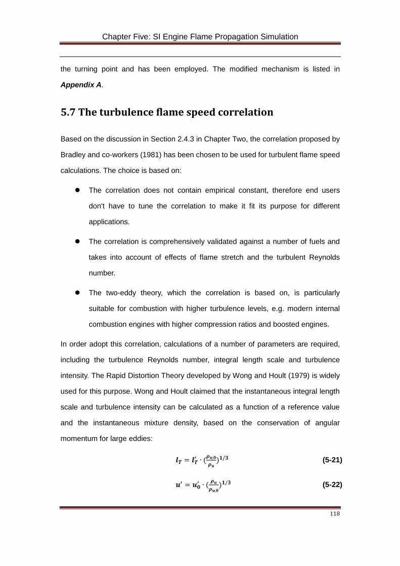
Chapter Five: SI Engine Flame Propagation Simulation
118
the turning point and has been employed. The modified mechanism is listed in
Appendix A.
5.7 The turbulence flame speed correlation
Based on the discussion in Section 2.4.3 in Chapter Two, the correlation proposed by
Bradley and co-workers (1981) has been chosen to be used for turbulent flame speed
calculations. The choice is based on:
The correlation does not contain empirical constant, therefore end users
don't have to tune the correlation to make it fit its purpose for different
applications.
The correlation is comprehensively validated against a number of fuels and
takes into account of effects of flame stretch and the turbulent Reynolds
number.
The two-eddy theory, which the correlation is based on, is particularly
suitable for combustion with higher turbulence levels, e.g. modern internal
combustion engines with higher compression ratios and boosted engines.
In order adopt this correlation, calculations of a number of parameters are required,
including the turbulence Reynolds number, integral length scale and turbulence
intensity. The Rapid Distortion Theory developed by Wong and Hoult (1979) is widely
used for this purpose. Wong and Hoult claimed that the instantaneous integral length
scale and turbulence intensity can be calculated as a function of a reference value
and the instantaneous mixture density, based on the conservation of angular
momentum for large eddies:
𝒍𝑻 = 𝒍𝑻′ ∙ (𝝆𝒖,𝟎𝝆𝒖
)𝟏/𝟑 (5-21)
𝒖′ = 𝒖𝟎′ ∙ ( 𝝆𝒖𝝆𝒖,𝟎
)𝟏/𝟑 (5-22)
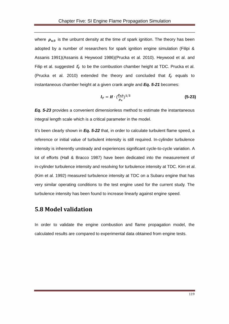
Chapter Five: SI Engine Flame Propagation Simulation
119
where 𝝆𝒖,𝟎 is the unburnt density at the time of spark ignition. The theory has been
adopted by a number of researchers for spark ignition engine simulation (Filipi &
Assanis 1991)(Assanis & Heywood 1986)(Prucka et al. 2010). Heywood et al. and
Filip et al. suggested 𝒍𝑻′ to be the combustion chamber height at TDC. Prucka et al.
(Prucka et al. 2010) extended the theory and concluded that 𝒍𝑻′ equals to
instantaneous chamber height at a given crank angle and Eq. 5-21 becomes:
𝒍𝑻 = 𝑯 ∙ (𝝆𝒖,𝟎𝝆𝒖
)𝟏/𝟑 (5-23)
Eq. 5-23 provides a convenient dimensionless method to estimate the instantaneous
integral length scale which is a critical parameter in the model.
It’s been clearly shown in Eq. 5-22 that, in order to calculate turbulent flame speed, a
reference or initial value of turbulent intensity is still required. In-cylinder turbulence
intensity is inherently unsteady and experiences significant cycle-to-cycle variation. A
lot of efforts (Hall & Bracco 1987) have been dedicated into the measurement of
in-cylinder turbulence intensity and resolving for turbulence intensity at TDC. Kim et al.
(Kim et al. 1992) measured turbulence intensity at TDC on a Subaru engine that has
very similar operating conditions to the test engine used for the current study. The
turbulence intensity has been found to increase linearly against engine speed.
5.8 Model validation
In order to validate the engine combustion and flame propagation model, the
calculated results are compared to experimental data obtained from engine tests.
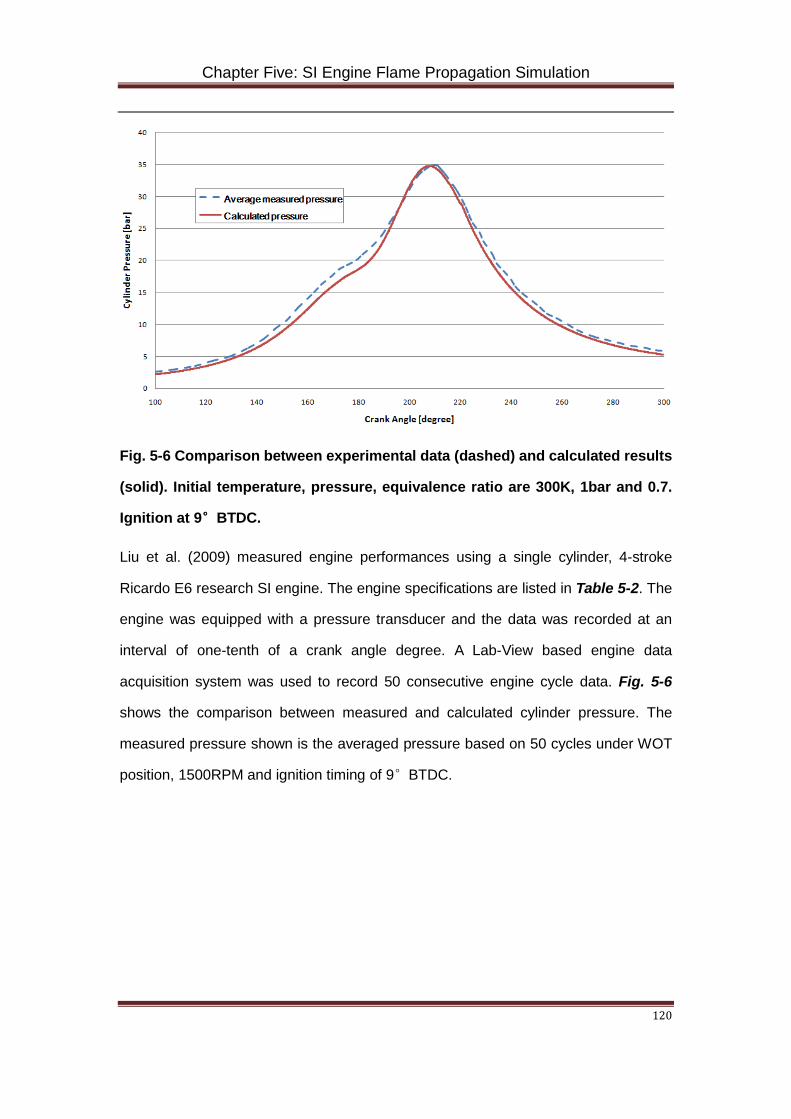
Chapter Five: SI Engine Flame Propagation Simulation
120
Fig. 5-6 Comparison between experimental data (dashed) and calculated results
(solid). Initial temperature, pressure, equivalence ratio are 300K, 1bar and 0.7.
Ignition at 9°BTDC.
Liu et al. (2009) measured engine performances using a single cylinder, 4-stroke
Ricardo E6 research SI engine. The engine specifications are listed in Table 5-2. The
engine was equipped with a pressure transducer and the data was recorded at an
interval of one-tenth of a crank angle degree. A Lab-View based engine data
acquisition system was used to record 50 consecutive engine cycle data. Fig. 5-6
shows the comparison between measured and calculated cylinder pressure. The
measured pressure shown is the averaged pressure based on 50 cycles under WOT
position, 1500RPM and ignition timing of 9°BTDC.
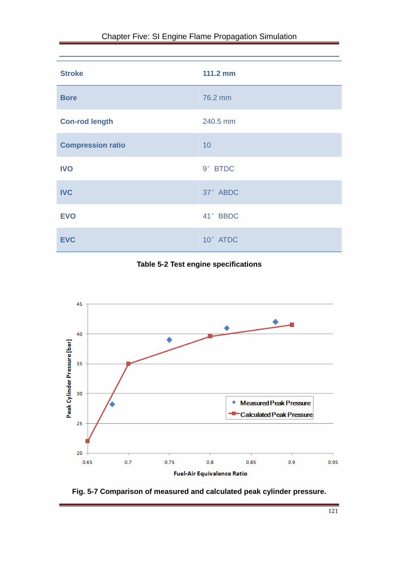
Chapter Five: SI Engine Flame Propagation Simulation
121
Stroke 111.2 mm
Bore 76.2 mm
Con-rod length 240.5 mm
Compression ratio 10
IVO 9°BTDC
IVC 37°ABDC
EVO 41°BBDC
EVC 10°ATDC
Table 5-2 Test engine specifications
Fig. 5-7 Comparison of measured and calculated peak cylinder pressure.
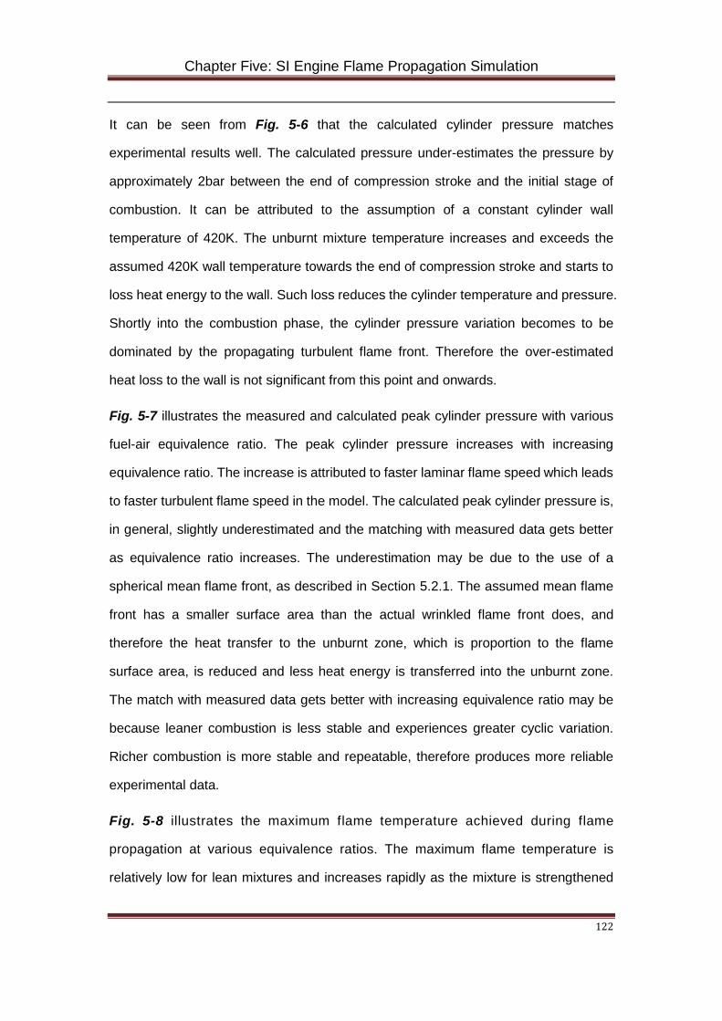
Chapter Five: SI Engine Flame Propagation Simulation
122
It can be seen from Fig. 5-6 that the calculated cylinder pressure matches
experimental results well. The calculated pressure under-estimates the pressure by
approximately 2bar between the end of compression stroke and the initial stage of
combustion. It can be attributed to the assumption of a constant cylinder wall
temperature of 420K. The unburnt mixture temperature increases and exceeds the
assumed 420K wall temperature towards the end of compression stroke and starts to
loss heat energy to the wall. Such loss reduces the cylinder temperature and pressure.
Shortly into the combustion phase, the cylinder pressure variation becomes to be
dominated by the propagating turbulent flame front. Therefore the over-estimated
heat loss to the wall is not significant from this point and onwards.
Fig. 5-7 illustrates the measured and calculated peak cylinder pressure with various
fuel-air equivalence ratio. The peak cylinder pressure increases with increasing
equivalence ratio. The increase is attributed to faster laminar flame speed which leads
to faster turbulent flame speed in the model. The calculated peak cylinder pressure is,
in general, slightly underestimated and the matching with measured data gets better
as equivalence ratio increases. The underestimation may be due to the use of a
spherical mean flame front, as described in Section 5.2.1. The assumed mean flame
front has a smaller surface area than the actual wrinkled flame front does, and
therefore the heat transfer to the unburnt zone, which is proportion to the flame
surface area, is reduced and less heat energy is transferred into the unburnt zone.
The match with measured data gets better with increasing equivalence ratio may be
because leaner combustion is less stable and experiences greater cyclic variation.
Richer combustion is more stable and repeatable, therefore produces more reliable
experimental data.
Fig. 5-8 illustrates the maximum flame temperature achieved during flame
propagation at various equivalence ratios. The maximum flame temperature is
relatively low for lean mixtures and increases rapidly as the mixture is strengthened
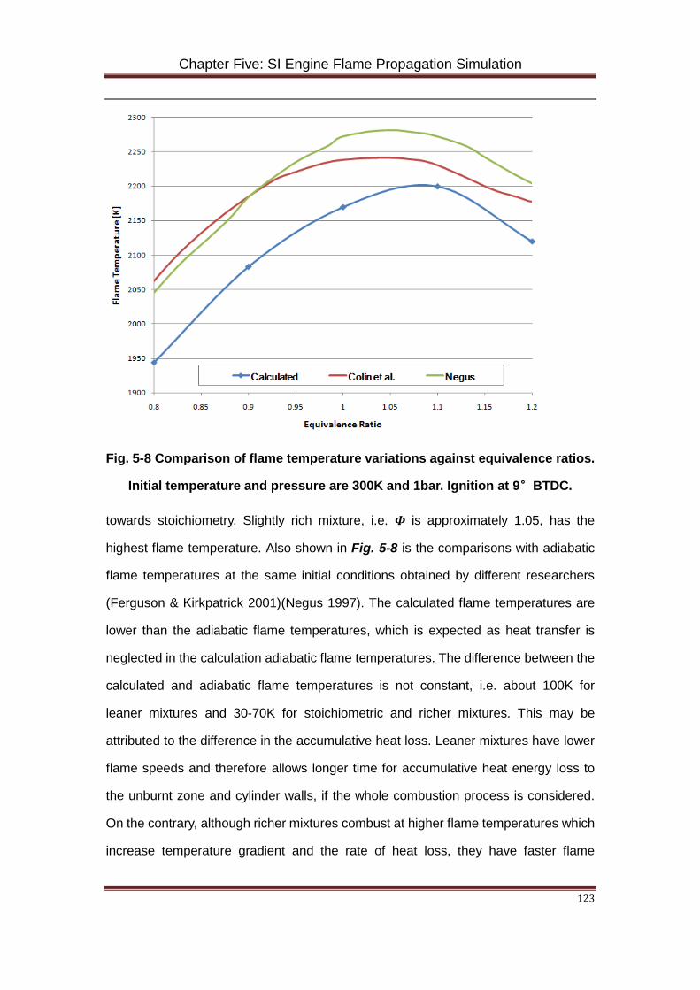
Chapter Five: SI Engine Flame Propagation Simulation
123
Fig. 5-8 Comparison of flame temperature variations against equivalence ratios.
Initial temperature and pressure are 300K and 1bar. Ignition at 9°BTDC.
towards stoichiometry. Slightly rich mixture, i.e. Ф is approximately 1.05, has the
highest flame temperature. Also shown in Fig. 5-8 is the comparisons with adiabatic
flame temperatures at the same initial conditions obtained by different researchers
(Ferguson & Kirkpatrick 2001)(Negus 1997). The calculated flame temperatures are
lower than the adiabatic flame temperatures, which is expected as heat transfer is
neglected in the calculation adiabatic flame temperatures. The difference between the
calculated and adiabatic flame temperatures is not constant, i.e. about 100K for
leaner mixtures and 30-70K for stoichiometric and richer mixtures. This may be
attributed to the difference in the accumulative heat loss. Leaner mixtures have lower
flame speeds and therefore allows longer time for accumulative heat energy loss to
the unburnt zone and cylinder walls, if the whole combustion process is considered.
On the contrary, although richer mixtures combust at higher flame temperatures which
increase temperature gradient and the rate of heat loss, they have faster flame
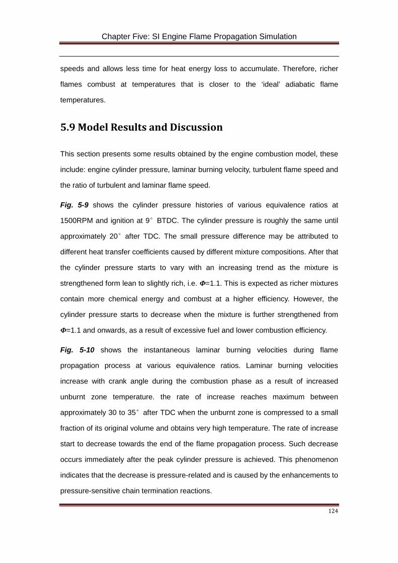
Chapter Five: SI Engine Flame Propagation Simulation
124
speeds and allows less time for heat energy loss to accumulate. Therefore, richer
flames combust at temperatures that is closer to the ‘ideal’ adiabatic flame
temperatures.
5.9 Model Results and Discussion
This section presents some results obtained by the engine combustion model, these
include: engine cylinder pressure, laminar burning velocity, turbulent flame speed and
the ratio of turbulent and laminar flame speed.
Fig. 5-9 shows the cylinder pressure histories of various equivalence ratios at
1500RPM and ignition at 9°BTDC. The cylinder pressure is roughly the same until
approximately 20°after TDC. The small pressure difference may be attributed to
different heat transfer coefficients caused by different mixture compositions. After that
the cylinder pressure starts to vary with an increasing trend as the mixture is
strengthened form lean to slightly rich, i.e. Ф=1.1. This is expected as richer mixtures
contain more chemical energy and combust at a higher efficiency. However, the
cylinder pressure starts to decrease when the mixture is further strengthened from
Ф=1.1 and onwards, as a result of excessive fuel and lower combustion efficiency.
Fig. 5-10 shows the instantaneous laminar burning velocities during flame
propagation process at various equivalence ratios. Laminar burning velocities
increase with crank angle during the combustion phase as a result of increased
unburnt zone temperature. the rate of increase reaches maximum between
approximately 30 to 35°after TDC when the unburnt zone is compressed to a small
fraction of its original volume and obtains very high temperature. The rate of increase
start to decrease towards the end of the flame propagation process. Such decrease
occurs immediately after the peak cylinder pressure is achieved. This phenomenon
indicates that the decrease is pressure-related and is caused by the enhancements to
pressure-sensitive chain termination reactions.
Chapter Five: SI Engine Flame Propagation Simulation
125
Fig. 5-9 Calculated cylinder pressure at various equivalence ratios. Initial
temperature and pressure are 300K and 1bar. Ignition at 9°BTDC.
Fig. 5-10 Calculated laminar burning velocity during the combustion phase at
various equivalence ratios. Initial temperature and pressure are 300K and 1bar.
Ignition at 9°BTDC.
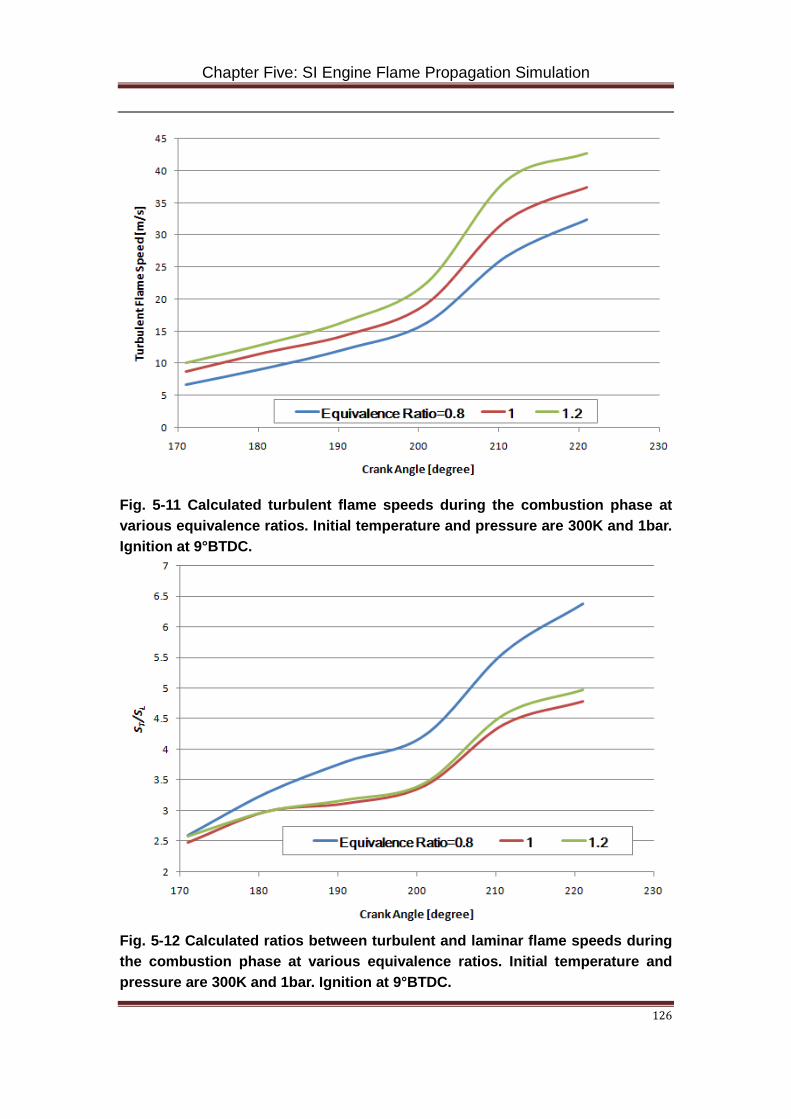
Chapter Five: SI Engine Flame Propagation Simulation
126
Fig. 5-11 Calculated turbulent flame speeds during the combustion phase at various equivalence ratios. Initial temperature and pressure are 300K and 1bar. Ignition at 9°BTDC.
Fig. 5-12 Calculated ratios between turbulent and laminar flame speeds during the combustion phase at various equivalence ratios. Initial temperature and pressure are 300K and 1bar. Ignition at 9°BTDC.
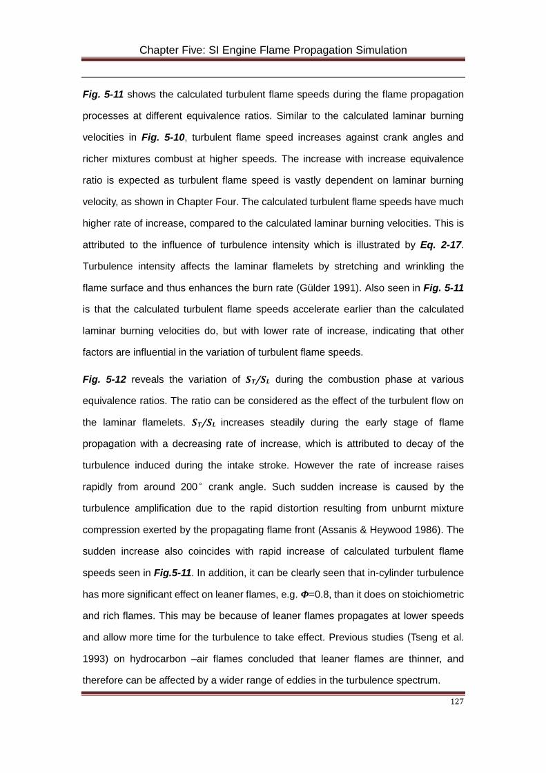
Chapter Five: SI Engine Flame Propagation Simulation
127
Fig. 5-11 shows the calculated turbulent flame speeds during the flame propagation
processes at different equivalence ratios. Similar to the calculated laminar burning
velocities in Fig. 5-10, turbulent flame speed increases against crank angles and
richer mixtures combust at higher speeds. The increase with increase equivalence
ratio is expected as turbulent flame speed is vastly dependent on laminar burning
velocity, as shown in Chapter Four. The calculated turbulent flame speeds have much
higher rate of increase, compared to the calculated laminar burning velocities. This is
attributed to the influence of turbulence intensity which is illustrated by Eq. 2-17.
Turbulence intensity affects the laminar flamelets by stretching and wrinkling the
flame surface and thus enhances the burn rate (Gülder 1991). Also seen in Fig. 5-11
is that the calculated turbulent flame speeds accelerate earlier than the calculated
laminar burning velocities do, but with lower rate of increase, indicating that other
factors are influential in the variation of turbulent flame speeds.
Fig. 5-12 reveals the variation of ST/SL during the combustion phase at various
equivalence ratios. The ratio can be considered as the effect of the turbulent flow on
the laminar flamelets. ST/SL increases steadily during the early stage of flame
propagation with a decreasing rate of increase, which is attributed to decay of the
turbulence induced during the intake stroke. However the rate of increase raises
rapidly from around 200°crank angle. Such sudden increase is caused by the
turbulence amplification due to the rapid distortion resulting from unburnt mixture
compression exerted by the propagating flame front (Assanis & Heywood 1986). The
sudden increase also coincides with rapid increase of calculated turbulent flame
speeds seen in Fig.5-11. In addition, it can be clearly seen that in-cylinder turbulence
has more significant effect on leaner flames, e.g. Ф=0.8, than it does on stoichiometric
and rich flames. This may be because of leaner flames propagates at lower speeds
and allow more time for the turbulence to take effect. Previous studies (Tseng et al.
1993) on hydrocarbon –air flames concluded that leaner flames are thinner, and
therefore can be affected by a wider range of eddies in the turbulence spectrum.
Chapter Five: SI Engine Flame Propagation Simulation
128
5.10 Summary
Turbulent flame propagation process plays an important role in spark ignition
combustion. It has dominating effect on combustion efficiency and cyclic variations. In
this chapter, a simulation model has been developed to study turbulent flame
propagation in spark ignition engines. The model is based on the zero-dimensional
approach and consists of three zones, i.e. burnt, burning and unburnt. A modified
chemical kinetics mechanism, originally developed by Tanaka and co-workers, has
been applied in the burning zone to simulate the in-flame combustion. The calculated
results have been validated against available experimental data for cylinder pressure
history, maximum cylinder pressure and maximum flame temperature.
The model has shown the ability of calculating instantaneous turbulent flame speeds
based on the wrinkled flamelet combustion regime where the combustion and the
turbulence are predicted separately. Both laminar burning velocities and turbulent
flame speeds are found to increase with increasing equivalence ratios from lean to
slightly rich conditions. The effects of the turbulence intensity are plotted and
discussed. It has been revealed that turbulence flow has more significant effects on
leaner flames which travel at lower flame speeds and are influenced by a wider range
of eddies in the turbulence spectrum.
The model also shows potential of being modified to study abnormal combustion
phenomenon, i.e. knock, in spark ignition engines, due to the zonal formation of the
model and the available gasoline combustion chemical kinetics mechanism. In the
next chapter, the model will be modified and used to study the knock phenomenon.
Chapter Six: Downsized Boosted SI Engine Knock Simulation
129
Chapter Six: Downsized Boosted SI Engine
Knock Simulation
6.1 Introduction
Design of modern spark ignition engines are significantly influenced by stringent
emission regulations and growing customers’ demand for lower running costs.
Downsizing and intake boosting have become the short-to-medium term solution for
major car manufacturers. By downsizing an engine, it is pushed to operate at higher
engine load and therefore has higher efficiency. The power and torque losses due to
reduction of wept volume is compensated by intake boosting, e.g. turbocharging and
supercharging. With these new engine designs, has come a growing concern for the
understanding, control and avoidance of end gas autoignition and the resultant knock
(Blunsdon & Dent 1994).
It is widely accepted that the propagating flame front is one of the most important
factors that contribute to the occurrence of end gas autoignition and knock. The
propagating flame front influence end gas autoignition and knock by increasing
unburnt mixture temperature and pressure by compression and heat convection.
Rapid compression and excessive heat convection to the unburnt mixture and easily
trigger autoignition and the resultant knock with high intensity. However, due to its
complexity and extremely transient nature, the relation and interaction between flame
propagation and knock are still not thoroughly understood.
In previous chapter, a spark ignition engine turbulent flame propagation model has
been developed and validated. The model is capable of predicting turbulent flame
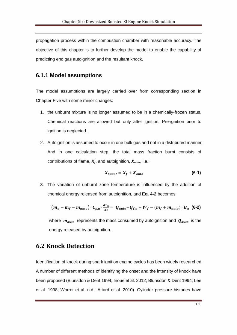
Chapter Six: Downsized Boosted SI Engine Knock Simulation
130
propagation process within the combustion chamber with reasonable accuracy. The
objective of this chapter is to further develop the model to enable the capability of
predicting end gas autoignition and the resultant knock.
6.1.1 Model assumptions
The model assumptions are largely carried over from corresponding section in
Chapter Five with some minor changes:
1. the unburnt mixture is no longer assumed to be in a chemically-frozen status.
Chemical reactions are allowed but only after ignition. Pre-ignition prior to
ignition is neglected.
2. Autoignition is assumed to occur in one bulk gas and not in a distributed manner.
And in one calculation step, the total mass fraction burnt consists of
contributions of flame, Xf, and autoignition, Xauto, i.e.:
𝑿𝒃𝒃𝒃𝒃𝒃 = 𝑿𝒇 + 𝑿𝒂𝒃𝒃𝒂 (6-1)
3. The variation of unburnt zone temperature is influenced by the addition of
chemical energy released from autoignition, and Eq. 4-2 becomes:
�𝒎𝒃 −𝒎𝒇 −𝒎𝒂𝒃𝒃𝒂� ∙ 𝑪𝒑,𝒃 ∙𝒅𝑻𝒃𝒅𝒃
= 𝑸𝒂𝒃𝒃𝒂̇ +𝑸𝒇,𝒃̇ + 𝑾𝒇̇ − (𝒎𝒇 +𝒎𝒂𝒃𝒃𝒂) ∙ 𝑯𝒃 (6-2)
where 𝒎𝒂𝒃𝒃𝒂 represents the mass consumed by autoignition and 𝑸𝒂𝒃𝒃𝒂 is the
energy released by autoignition.
6.2 Knock Detection
Identification of knock during spark ignition engine cycles has been widely researched.
A number of different methods of identifying the onset and the intensity of knock have
been proposed (Blunsdon & Dent 1994; Inoue et al. 2012; Blunsdon & Dent 1994; Lee
et al. 1998; Worret et al. n.d.; Attard et al. 2010). Cylinder pressure histories have
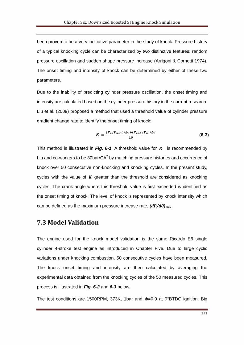
Chapter Six: Downsized Boosted SI Engine Knock Simulation
131
been proven to be a very indicative parameter in the study of knock. Pressure history
of a typical knocking cycle can be characterized by two distinctive features: random
pressure oscillation and sudden shape pressure increase (Arrigoni & Cornetti 1974).
The onset timing and intensity of knock can be determined by either of these two
parameters.
Due to the inability of predicting cylinder pressure oscillation, the onset timing and
intensity are calculated based on the cylinder pressure history in the current research.
Liu et al. (2009) proposed a method that used a threshold value of cylinder pressure
gradient change rate to identify the onset timing of knock:
𝑲 = (𝑷𝒃 𝑷𝒃−𝟏⁄ )/∆𝜽+(𝑷𝒃+𝟏 𝑷𝒃⁄ )/∆𝜽∆𝜽
(6-3)
This method is illustrated in Fig. 6-1. A threshold value for 𝑲 is recommended by
Liu and co-workers to be 30bar/CA2 by matching pressure histories and occurrence of
knock over 50 consecutive non-knocking and knocking cycles. In the present study,
cycles with the value of 𝑲 greater than the threshold are considered as knocking
cycles. The crank angle where this threshold value is first exceeded is identified as
the onset timing of knock. The level of knock is represented by knock intensity which
can be defined as the maximum pressure increase rate, (dP/dθ)max.
7.3 Model Validation
The engine used for the knock model validation is the same Ricardo E6 single
cylinder 4-stroke test engine as introduced in Chapter Five. Due to large cyclic
variations under knocking combustion, 50 consecutive cycles have been measured.
The knock onset timing and intensity are then calculated by averaging the
experimental data obtained from the knocking cycles of the 50 measured cycles. This
process is illustrated in Fig. 6-2 and 6-3 below.
The test conditions are 1500RPM, 373K, 1bar and Ф=0.9 at 9°BTDC ignition. Big
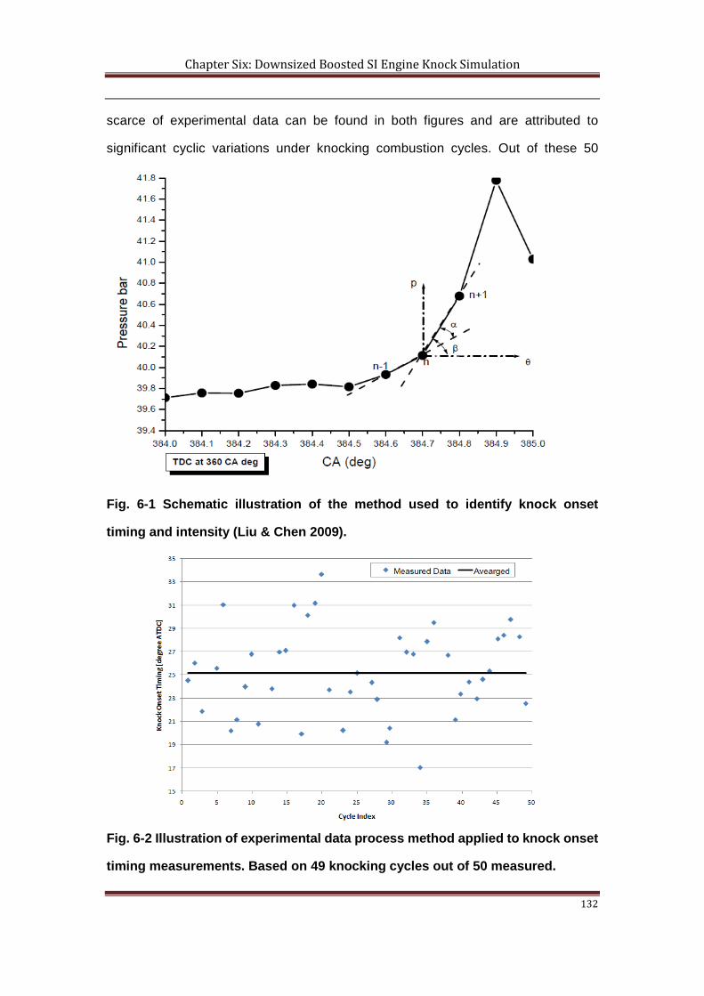
Chapter Six: Downsized Boosted SI Engine Knock Simulation
132
scarce of experimental data can be found in both figures and are attributed to
significant cyclic variations under knocking combustion cycles. Out of these 50
Fig. 6-1 Schematic illustration of the method used to identify knock onset
timing and intensity (Liu & Chen 2009).
Fig. 6-2 Illustration of experimental data process method applied to knock onset
timing measurements. Based on 49 knocking cycles out of 50 measured.
Chapter Six: Downsized Boosted SI Engine Knock Simulation
133
Fig. 6-3 Illustration of experimental data process method applied to knock
intensity measurements. Based on 49 knocking cycles out of 50 measured.
measured cycles, 49 are knocking cycles and 1 is considered to be knock-free. The
averaged values are obtained by adding measured data and dividing the number of
knocking cycles.
Fig. 6-4 shows the comparisons of calculated and measured knock onset timing and
intensity at different engine speeds. It can be clearly seen that as the engine speed is
increased, knock onset timing is delayed and knock intensity is reduced, both in a
almost linear manner. Engine speed determines the time available for the combustion
phase. Due to its kinetically-controlled and time-dependent nature, knock (end gas
autoignition) is logically delayed as engine speed increases. The reduction in knock
intensity may be attributed to the fact that the compression exerted by the propagating
flame front on unburnt mixture is growingly offset by the faster downward motion of
piston during the expansion stroke, as the engine speed is increased. The match with
measured results is acceptable and the model has been proven to be able to simulate
spark ignition engine autoignition and knock.
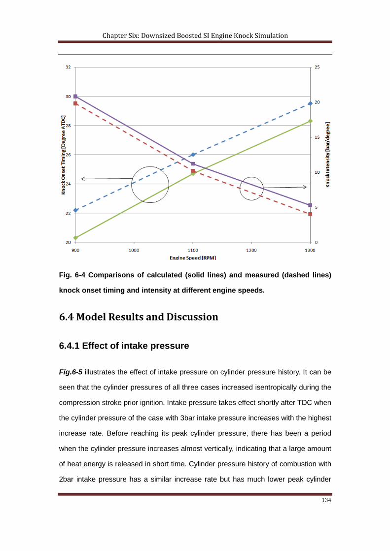
Chapter Six: Downsized Boosted SI Engine Knock Simulation
134
Fig. 6-4 Comparisons of calculated (solid lines) and measured (dashed lines)
knock onset timing and intensity at different engine speeds.
6.4 Model Results and Discussion
6.4.1 Effect of intake pressure
Fig.6-5 illustrates the effect of intake pressure on cylinder pressure history. It can be
seen that the cylinder pressures of all three cases increased isentropically during the
compression stroke prior ignition. Intake pressure takes effect shortly after TDC when
the cylinder pressure of the case with 3bar intake pressure increases with the highest
increase rate. Before reaching its peak cylinder pressure, there has been a period
when the cylinder pressure increases almost vertically, indicating that a large amount
of heat energy is released in short time. Cylinder pressure history of combustion with
2bar intake pressure has a similar increase rate but has much lower peak cylinder
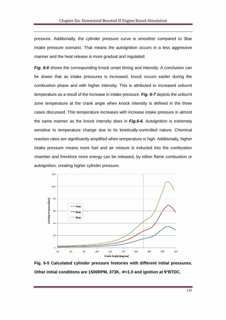
Chapter Six: Downsized Boosted SI Engine Knock Simulation
135
pressure. Additionally, the cylinder pressure curve is smoother compared to 3bar
intake pressure scenario. That means the autoignition occurs in a less aggressive
manner and the heat release is more gradual and regulated.
Fig. 6-6 shows the corresponding knock onset timing and intensity. A conclusion can
be drawn that as intake pressures is increased, knock occurs earlier during the
combustion phase and with higher intensity. This is attributed to increased unburnt
temperature as a result of the increase in intake pressure. Fig. 6-7 depicts the unburnt
zone temperature at the crank angle when knock intensity is defined in the three
cases discussed. This temperature increases with increase intake pressure in almost
the same manner as the knock intensity does in Fig.6-6. Autoignition is extremely
sensitive to temperature change due to its kinetically-controlled nature. Chemical
reaction rates are significantly amplified when temperature is high. Additionally, higher
intake pressure means more fuel and air mixture is inducted into the combustion
chamber and therefore more energy can be released, by either flame combustion or
autoignition, creating higher cylinder pressure.
Fig. 6-5 Calculated cylinder pressure histories with different initial pressures.
Other initial conditions are 1500RPM, 373K, Ф=1.0 and ignition at 9°BTDC.
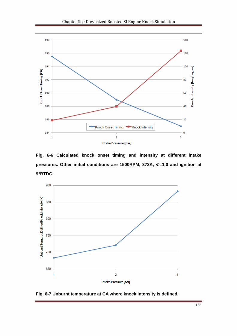
Chapter Six: Downsized Boosted SI Engine Knock Simulation
136
Fig. 6-6 Calculated knock onset timing and intensity at different intake
pressures. Other initial conditions are 1500RPM, 373K, Ф=1.0 and ignition at
9°BTDC.
Fig. 6-7 Unburnt temperature at CA where knock intensity is defined.
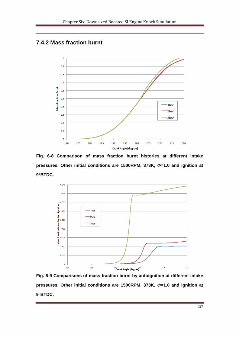
Chapter Six: Downsized Boosted SI Engine Knock Simulation
137
7.4.2 Mass fraction burnt
Fig. 6-8 Comparison of mass fraction burnt histories at different intake
pressures. Other initial conditions are 1500RPM, 373K, Ф=1.0 and ignition at
9°BTDC.
Fig. 6-9 Comparisons of mass fraction burnt by autoignition at different intake
pressures. Other initial conditions are 1500RPM, 373K, Ф=1.0 and ignition at
9°BTDC.
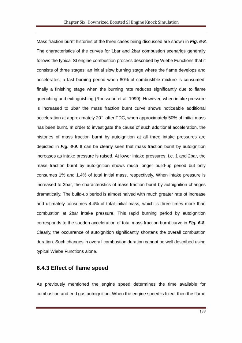
Chapter Six: Downsized Boosted SI Engine Knock Simulation
138
Mass fraction burnt histories of the three cases being discussed are shown in Fig. 6-8.
The characteristics of the curves for 1bar and 2bar combustion scenarios generally
follows the typical SI engine combustion process described by Wiebe Functions that it
consists of three stages: an initial slow burning stage where the flame develops and
accelerates; a fast burning period when 80% of combustible mixture is consumed;
finally a finishing stage when the burning rate reduces significantly due to flame
quenching and extinguishing (Rousseau et al. 1999). However, when intake pressure
is increased to 3bar the mass fraction burnt curve shows noticeable additional
acceleration at approximately 20°after TDC, when approximately 50% of initial mass
has been burnt. In order to investigate the cause of such additional acceleration, the
histories of mass fraction burnt by autoignition at all three intake pressures are
depicted in Fig. 6-9. It can be clearly seen that mass fraction burnt by autoignition
increases as intake pressure is raised. At lower intake pressures, i.e. 1 and 2bar, the
mass fraction burnt by autoignition shows much longer build-up period but only
consumes 1% and 1.4% of total initial mass, respectively. When intake pressure is
increased to 3bar, the characteristics of mass fraction burnt by autoignition changes
dramatically. The build-up period is almost halved with much greater rate of increase
and ultimately consumes 4.4% of total initial mass, which is three times more than
combustion at 2bar intake pressure. This rapid burning period by autoignition
corresponds to the sudden acceleration of total mass fraction burnt curve in Fig. 6-8.
Clearly, the occurrence of autoignition significantly shortens the overall combustion
duration. Such changes in overall combustion duration cannot be well described using
typical Wiebe Functions alone.
6.4.3 Effect of flame speed
As previously mentioned the engine speed determines the time available for
combustion and end gas autoignition. When the engine speed is fixed, then the flame
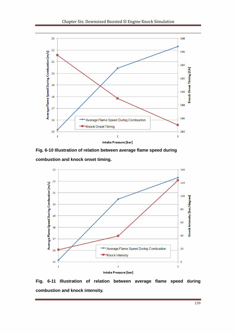
Chapter Six: Downsized Boosted SI Engine Knock Simulation
139
Fig. 6-10 Illustration of relation between average flame speed during
combustion and knock onset timing.
Fig. 6-11 Illustration of relation between average flame speed during
combustion and knock intensity.
Chapter Six: Downsized Boosted SI Engine Knock Simulation
140
speed becomes the dominating time scale for combustion and end gas autoignition. It
is necessary to investigate the relation between flame propagation and knock. Fig.
6-10 and 6-11 show the relations between average flame speed and knock onset
timing, and knock intensity, respectively. Initial conditions are 373K, stoichiometric
mixture and ignition at 9°BTDC. The average flame speed is obtained by adding
calculated turbulent flame speed at each crank angle and divide the sum by number
of crank angles of the combustion phase. Average flame speed has been chosen over
peak flame speed because it is more indicative when being used as indication of time
availability for autoignition.
6.5 Summary
It can be clearly seen that average flame speed increases with increasing intake
pressure. This is mainly attributed to the correspondent temperature increase
resultant from the intake pressure change. As described in Chapter Five, the
calculated turbulent flame speed consists of a chemical-kinetics-based laminar flame
speed and a laminar-to-turbulent flame speed correlation. Therefore, as the unburnt
temperature raises the laminar flame speed is increased, and so does the turbulent
flame speed. However such increase of turbulent flame speed is not linear against
intake pressure variation, i.e. 35.9% increase in average flame speed is achieved by
increasing intake pressure from 1bar to 2bar, but only 9% has been achieved when
it’s been further increased to 3bar. This may be because when intake pressure is
raised to 3bar, cylinder pressure during later stage of combustion is sufficiently high
for pressure-sensitive chain termination reactions to become dominant over
temperature-sensitive chain branching reactions, and thus reduces the laminar flame
speed. Additionally, the turbulence intensity is assumed to be a function of only its
reference value and crank angle, i.e. independent of temperature and pressure
change. Therefore the increase rate of average flame speed is lowering as intake
Chapter Six: Downsized Boosted SI Engine Knock Simulation
141
pressure is increased.
Also shown in Fig. 6-10 and 6-11 is that, as average flame speed is increased, knock
onset timing is advanced and knock intensity is amplified. Theoretically, faster
average flame speed should allow less time for autoignition to build up and develop
into knock, or reduce knock intensity if it does develop into a knocking cycle. However,
such phenomenon has not been replicated in the simulation results. This finding
indicates that, in practical application, increasing intake pressure without optimisation
of other engine operating parameters will increase flame speed and cylinder pressure
and, therefore, improve engine performance, but also induce severe knock problem,
making such operating strategy unfeasible. An optimized operating strategy that
allows higher intake pressures to improve engine performance but also, at the
meantime, keeps the knock in a controlled level should be further investigated.
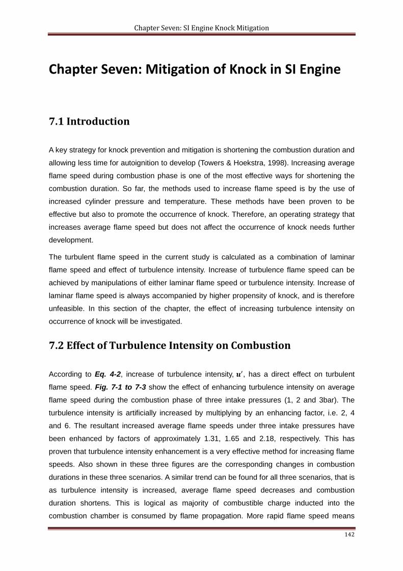
Chapter Seven: SI Engine Knock Mitigation
142
Chapter Seven: Mitigation of Knock in SI Engine
7.1 Introduction
A key strategy for knock prevention and mitigation is shortening the combustion duration and
allowing less time for autoignition to develop (Towers & Hoekstra, 1998). Increasing average
flame speed during combustion phase is one of the most effective ways for shortening the
combustion duration. So far, the methods used to increase flame speed is by the use of
increased cylinder pressure and temperature. These methods have been proven to be
effective but also to promote the occurrence of knock. Therefore, an operating strategy that
increases average flame speed but does not affect the occurrence of knock needs further
development.
The turbulent flame speed in the current study is calculated as a combination of laminar
flame speed and effect of turbulence intensity. Increase of turbulence flame speed can be
achieved by manipulations of either laminar flame speed or turbulence intensity. Increase of
laminar flame speed is always accompanied by higher propensity of knock, and is therefore
unfeasible. In this section of the chapter, the effect of increasing turbulence intensity on
occurrence of knock will be investigated.
7.2 Effect of Turbulence Intensity on Combustion
According to Eq. 4-2, increase of turbulence intensity, 𝒖′, has a direct effect on turbulent
flame speed. Fig. 7-1 to 7-3 show the effect of enhancing turbulence intensity on average
flame speed during the combustion phase of three intake pressures (1, 2 and 3bar). The
turbulence intensity is artificially increased by multiplying by an enhancing factor, i.e. 2, 4
and 6. The resultant increased average flame speeds under three intake pressures have
been enhanced by factors of approximately 1.31, 1.65 and 2.18, respectively. This has
proven that turbulence intensity enhancement is a very effective method for increasing flame
speeds. Also shown in these three figures are the corresponding changes in combustion
durations in these three scenarios. A similar trend can be found for all three scenarios, that is
as turbulence intensity is increased, average flame speed decreases and combustion
duration shortens. This is logical as majority of combustible charge inducted into the
combustion chamber is consumed by flame propagation. More rapid flame speed means
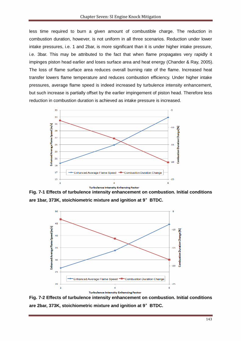
Chapter Seven: SI Engine Knock Mitigation
143
less time required to burn a given amount of combustible charge. The reduction in
combustion duration, however, is not uniform in all three scenarios. Reduction under lower
intake pressures, i.e. 1 and 2bar, is more significant than it is under higher intake pressure,
i.e. 3bar. This may be attributed to the fact that when flame propagates very rapidly it
impinges piston head earlier and loses surface area and heat energy (Chander & Ray, 2005).
The loss of flame surface area reduces overall burning rate of the flame. Increased heat
transfer lowers flame temperature and reduces combustion efficiency. Under higher intake
pressures, average flame speed is indeed increased by turbulence intensity enhancement,
but such increase is partially offset by the earlier impingement of piston head. Therefore less
reduction in combustion duration is achieved as intake pressure is increased.
Fig. 7-1 Effects of turbulence intensity enhancement on combustion. Initial conditions
are 1bar, 373K, stoichiometric mixture and ignition at 9°BTDC.
Fig. 7-2 Effects of turbulence intensity enhancement on combustion. Initial conditions
are 2bar, 373K, stoichiometric mixture and ignition at 9°BTDC.
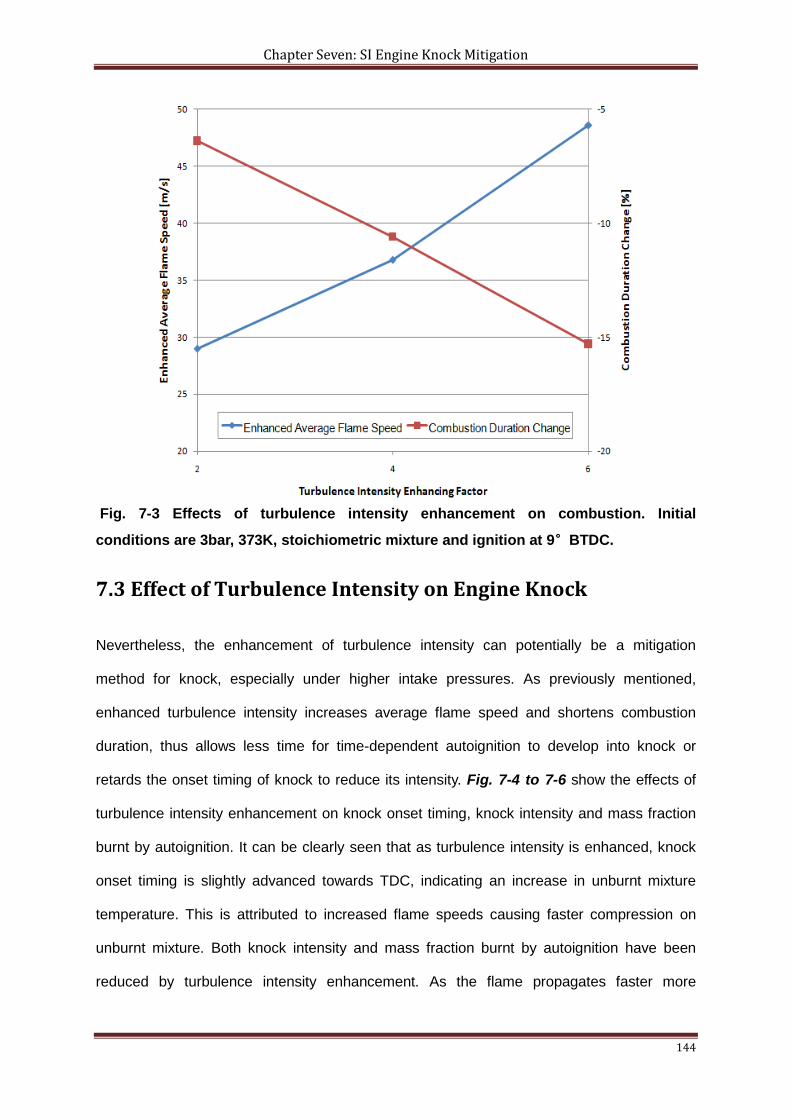
Chapter Seven: SI Engine Knock Mitigation
144
Fig. 7-3 Effects of turbulence intensity enhancement on combustion. Initial
conditions are 3bar, 373K, stoichiometric mixture and ignition at 9°BTDC.
7.3 Effect of Turbulence Intensity on Engine Knock
Nevertheless, the enhancement of turbulence intensity can potentially be a mitigation
method for knock, especially under higher intake pressures. As previously mentioned,
enhanced turbulence intensity increases average flame speed and shortens combustion
duration, thus allows less time for time-dependent autoignition to develop into knock or
retards the onset timing of knock to reduce its intensity. Fig. 7-4 to 7-6 show the effects of
turbulence intensity enhancement on knock onset timing, knock intensity and mass fraction
burnt by autoignition. It can be clearly seen that as turbulence intensity is enhanced, knock
onset timing is slightly advanced towards TDC, indicating an increase in unburnt mixture
temperature. This is attributed to increased flame speeds causing faster compression on
unburnt mixture. Both knock intensity and mass fraction burnt by autoignition have been
reduced by turbulence intensity enhancement. As the flame propagates faster more
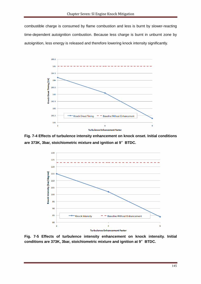
Chapter Seven: SI Engine Knock Mitigation
145
combustible charge is consumed by flame combustion and less is burnt by slower-reacting
time-dependent autoignition combustion. Because less charge is burnt in unburnt zone by
autoignition, less energy is released and therefore lowering knock intensity significantly.
Fig. 7-4 Effects of turbulence intensity enhancement on knock onset. Initial conditions
are 373K, 3bar, stoichiometric mixture and ignition at 9°BTDC.
Fig. 7-5 Effects of turbulence intensity enhancement on knock intensity. Initial conditions are 373K, 3bar, stoichiometric mixture and ignition at 9°BTDC.
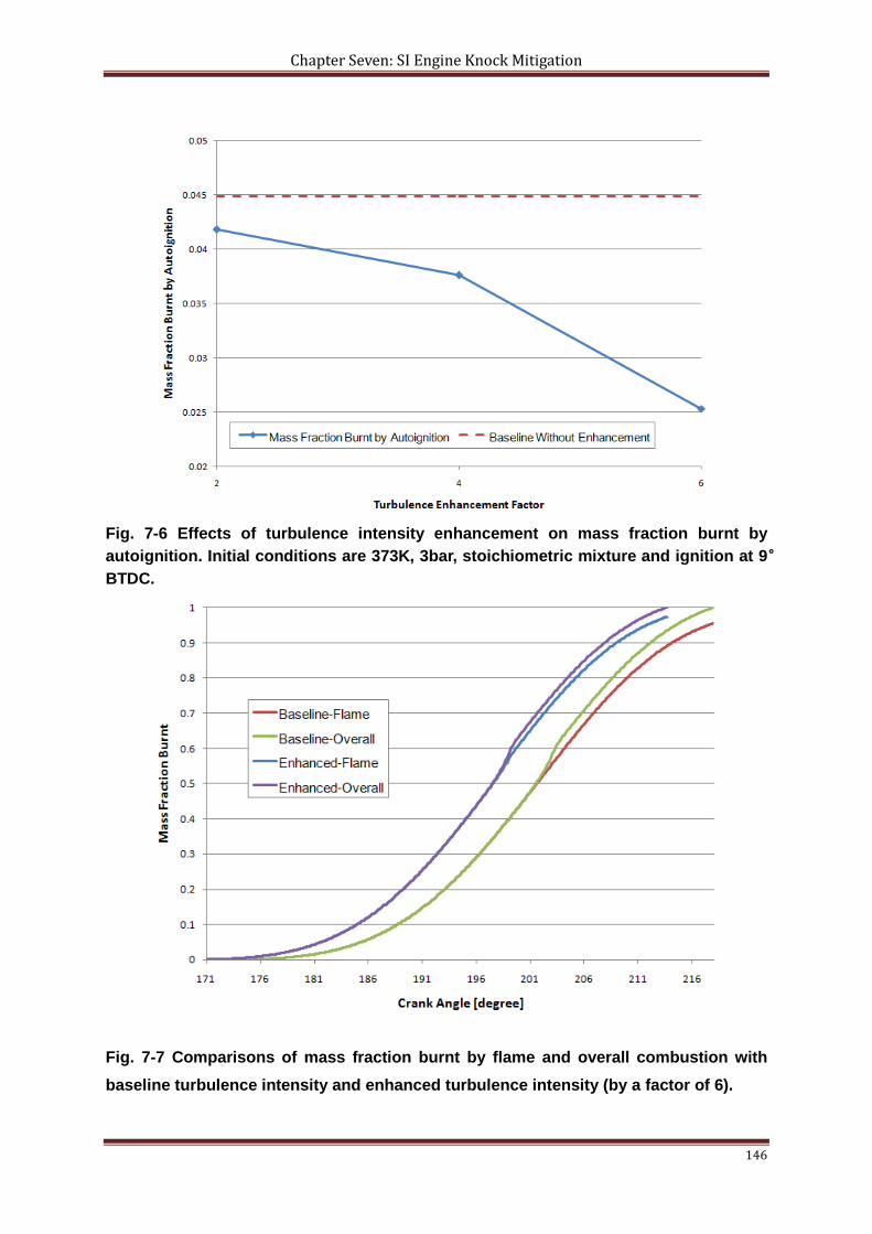
Chapter Seven: SI Engine Knock Mitigation
146
Fig. 7-6 Effects of turbulence intensity enhancement on mass fraction burnt by autoignition. Initial conditions are 373K, 3bar, stoichiometric mixture and ignition at 9°BTDC.
Fig. 7-7 Comparisons of mass fraction burnt by flame and overall combustion with baseline turbulence intensity and enhanced turbulence intensity (by a factor of 6).
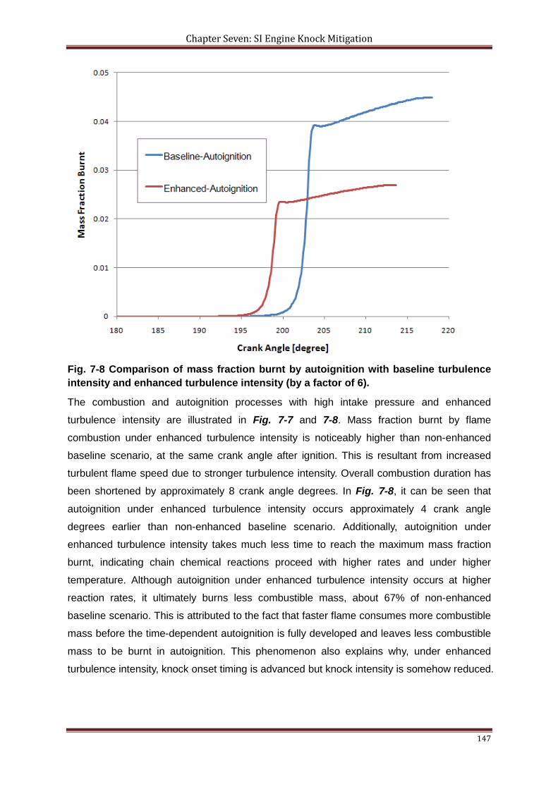
Chapter Seven: SI Engine Knock Mitigation
147
Fig. 7-8 Comparison of mass fraction burnt by autoignition with baseline turbulence intensity and enhanced turbulence intensity (by a factor of 6).
The combustion and autoignition processes with high intake pressure and enhanced
turbulence intensity are illustrated in Fig. 7-7 and 7-8. Mass fraction burnt by flame
combustion under enhanced turbulence intensity is noticeably higher than non-enhanced
baseline scenario, at the same crank angle after ignition. This is resultant from increased
turbulent flame speed due to stronger turbulence intensity. Overall combustion duration has
been shortened by approximately 8 crank angle degrees. In Fig. 7-8, it can be seen that
autoignition under enhanced turbulence intensity occurs approximately 4 crank angle
degrees earlier than non-enhanced baseline scenario. Additionally, autoignition under
enhanced turbulence intensity takes much less time to reach the maximum mass fraction
burnt, indicating chain chemical reactions proceed with higher rates and under higher
temperature. Although autoignition under enhanced turbulence intensity occurs at higher
reaction rates, it ultimately burns less combustible mass, about 67% of non-enhanced
baseline scenario. This is attributed to the fact that faster flame consumes more combustible
mass before the time-dependent autoignition is fully developed and leaves less combustible
mass to be burnt in autoignition. This phenomenon also explains why, under enhanced
turbulence intensity, knock onset timing is advanced but knock intensity is somehow reduced.
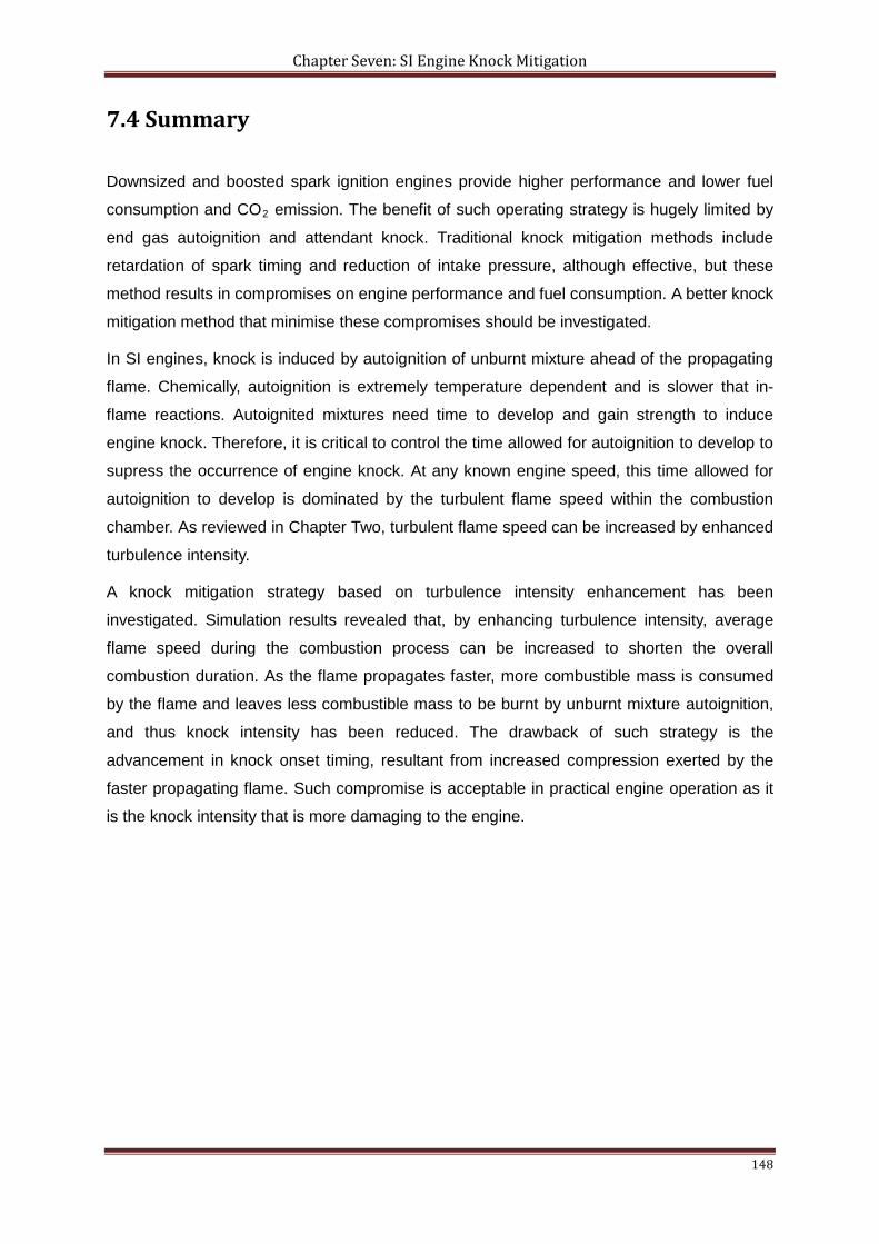
Chapter Seven: SI Engine Knock Mitigation
148
7.4 Summary
Downsized and boosted spark ignition engines provide higher performance and lower fuel
consumption and CO2 emission. The benefit of such operating strategy is hugely limited by
end gas autoignition and attendant knock. Traditional knock mitigation methods include
retardation of spark timing and reduction of intake pressure, although effective, but these
method results in compromises on engine performance and fuel consumption. A better knock
mitigation method that minimise these compromises should be investigated.
In SI engines, knock is induced by autoignition of unburnt mixture ahead of the propagating
flame. Chemically, autoignition is extremely temperature dependent and is slower that in-
flame reactions. Autoignited mixtures need time to develop and gain strength to induce
engine knock. Therefore, it is critical to control the time allowed for autoignition to develop to
supress the occurrence of engine knock. At any known engine speed, this time allowed for
autoignition to develop is dominated by the turbulent flame speed within the combustion
chamber. As reviewed in Chapter Two, turbulent flame speed can be increased by enhanced
turbulence intensity.
A knock mitigation strategy based on turbulence intensity enhancement has been
investigated. Simulation results revealed that, by enhancing turbulence intensity, average
flame speed during the combustion process can be increased to shorten the overall
combustion duration. As the flame propagates faster, more combustible mass is consumed
by the flame and leaves less combustible mass to be burnt by unburnt mixture autoignition,
and thus knock intensity has been reduced. The drawback of such strategy is the
advancement in knock onset timing, resultant from increased compression exerted by the
faster propagating flame. Such compromise is acceptable in practical engine operation as it
is the knock intensity that is more damaging to the engine.
Chapter Eight: Conclusions and Future Work
149
Chapter Eight: Conclusions and Future Work
8.1 Concluding remarks
The current research study has been focused on the development, validation and
application of two spark ignition engine models:
1. A naturally aspirated spark ignition engine combustion and flame propagation
model.
2. A downsized boosted spark ignition engine knock model.
Both models are developed based on zero-dimensional multi-zone modelling
philosophy, for the simulation of kinetically-driven combustion phenomenon within the
flame and in the unburnt mixtures.
The major contributions of this research study is primarily made to establish a
mathematical simulation model based on available physical, chemical,
thermodynamic and fluid dynamic principles of combustion ,flame propagation and
autoignition occur in spark ignition engines. The developed model is then solved by
an in-house numerical solver. The aims of this research study is to establish better
understanding of the transient turbulent flame propagation and its interaction with end
gas autoignition and the attendant knock in spark ignition engines. The simulation
model can be used as a diagnose tool for combustion and knock characteristics under
realistic in-cylinder conditions.
Both in-flame combustion and end gas autoignition in spark ignition engines are
chemical-kinetic-controlled. The difference is the ignition source where in-flame
combustion is initiated by external energy input, i.e. electrical spark, and is maintained
through mass diffusion and heat transfer. End gas autoignition, in contrary, is initiated
Chapter Eight: Conclusions and Future Work
150
by chemical reactions with heat release resultant from compression work by piston
motion and flame propagation. Therefore, chemical kinetics modelling has been
adopted to simulate both in-flame and autoignition combustion, which can be seen as
processes of hydrocarbon oxidation occurring at different time scales and intensities.
Zero-dimensional, multi-zone engine modelling has been widely used as a functional
simulation philosophy to study the combustion process in spark ignition engines. It
has been regarded as a optimal balance between computational accuracy and costs.
Combination of chemical kinetics models and zero-dimensional multi-zone
thermodynamics model is then a effective and efficient method of modelling turbulent
flame propagation and end gas autoignition phenomenon in spark ignition engines.
Additional benefits of zero-dimensional multi-zone modelling are briefly listed below:
Compared to single-zone models, multi-zone models account for
temperature, pressure and composition gradient within the combustion
chamber. It also enables the separation of a dedicated flame/burning zone to
study the flame propagation process.
Multi-zone models are capable of simulating mass and heat transfer between
burning and unburnt zone, which is critical in flame propagation mechanism.
Multi-zone models can be coupled with simplified mean turbulence models to
significantly reduce computational costs, when detailed in-cylinder flow
characteristics are not concerned.
In the development process of the model, some coding principles are bear in mind to
make the model more efficient and user-friendly:
The model has been written in programming language FORTRAN 77/90 to
make the codes transferable between computers and different operation
systems.
The model has been constructed in a modular structure where a relatively
Chapter Eight: Conclusions and Future Work
151
simple main program controls the data flow and calls for subroutines of
different functions. It is therefore easier to turn some of the functions of the
model on and off.
A DVODE (Double-precision Variable-coefficient Ordinary Differential
Equation) solver is applied to solve initial value problems for both stiff and
non-stiff ODEs systems.
8.1.1 SI engine turbulent flame modelling
Turbulent flame propagation within spark ignition engines is closely related to
combustion efficiency, fuel consumption, cyclic variation and abnormal combustion
phenomenon. Previous research work on turbulent flame propagation under
engine-like conditions is limited by its complexity and extremely random and transient
nature. In the current research, turbulent flame propagation within spark ignition
engines is assumed to fall into the wrinkle flamelet combustion regime. Therefore, the
combustion process and the effects of turbulence on reacting laminar flamelets can
be separately studied and modelled. The turbulent flame speed is then considered as
a combination of laminar flame speeds and contribution from critical turbulence
parameters, i.e. turbulence intensity.
The instantaneous turbulence intensity and other turbulence parameters at any given
crank angles are evaluated using the rapid distortion theory with reference values at
TDC position that are obtained experimentally.
Laminar flame speed is considered as a result of laminar burning velocity, flame
stretch, flame instabilities and thermal expansion. Laminar burning velocity is a
property of a fuel at given initial conditions, i.e. temperature, pressure and
composition. Laminar burning velocity is chemically-controlled and therefore modelled
using chemical kinetics mechanism. Such novel methodology has been firstly
validated by modelling of spherical flames in constant volume combustion chamber,
Chapter Eight: Conclusions and Future Work
152
before being applied in spark ignition engine turbulent flame modelling.
The interaction between turbulence and laminar flame speed has been described
using a established turbulence flame speed correlation. This correlation has been
selected by extensive review on available correlations by the criterion that it best suits
turbulence combustion under engine-like conditions which are characterised by
higher turbulence levels and increased turbulent Reynolds Number.
Some model-specific assumptions are applied to suit the development of the model:
The ignition process is neglected and a flame kernel is assumed to exist after
the breakdown period. The kernel initially propagates at the rate of laminar
flame speed under thermodynamic conditions at ignition. Pressure is
assumed to be uniform on both sides of kernel. Adopted values for kernel
size and breakdown period to be 1mm radius and 200μs respectively.
The turbulent flame front is assumed to have a spherical shape and such
shape is maintained throughout combustion. The instantaneous turbulent
flame front is arbitrarily wrinkled by the small eddies in the turbulent flow. A
mean flame front centre line is introduced to simplify the flame geometry, as
depicted in Fig. 6-2. The mean flame front has the same thickness as the
instantaneous flame front, which is denoted as 𝜹𝑻.
The turbulent intensity within the combustion chamber is assumed to be
spatially uniform. Additionally, the turbulence intensity is assumed to be a
function of crank angle and its reference value at TDC, at a given engine
speed.
Major contributions and findings of spark ignition engine turbulent flame modelling are
listed below:
Instantaneous laminar burning velocity increases during the flame
propagation process, as a result of increased unburnt zone temperature. The
increase rate of laminar flame speed is relatively low at initial stage of flame
Chapter Eight: Conclusions and Future Work
153
propagation. The rate increases suddenly and results in maximum laminar
flame speed between 30 to 35°ATDC when the unburnt zone is compressed
to a small fraction of its volume before ignition. The rate then starts to
decrease towards the end of the flame propagation process. Such decrease
has been attributed to pressure-sensitive chain termination reactions in the
chemical kinetics model.
Instantaneous turbulence flame speed increases with crank angle during the
combustion phase. Richer mixtures have higher turbulence flame speed
under simulated conditions (0.8<Ф<1.2). Increase rates of turbulent flame
speed are generally greater than those of laminar burning velocity at the
same crank angle. This is attributed to contributions of turbulence intensity.
Investigation of relation between turbulent and laminar flame speed, ST/SL,
revealed that leaner laminar flames are more sensitive to turbulence intensity
due to their relatively low flame speeds and thinner flame front. The effect of
turbulence intensity has been found to decrease in the initial stage of
combustion due to rapid decay. However, such effect starts to increase at
around 200°CA as a result of strong compression of unburnt mixture by
propagating flame.
8.1.2 Downsized boosted SI engine knock modelling
The current research also investigated the knock phenomenon in modern downsized
boosted spark ignition engines. A modified Tanaka chemical kinetics model for
gasoline has been applied to unburnt zone to simulate end gas autoignition. The
purpose for modification is to make the model suitable for spark ignition combustion,
as the original model was designed for HCCI combustion of gasoline. Reaction rates
of key chain branching elementary reactions R6 and R18 in the original model have
been amplified and validated to reproduce the characteristics of spark ignition
combustion, which are higher burning rate and shorter ignition delay.
Chapter Eight: Conclusions and Future Work
154
In order to simulate the effect of downsizing and boosting on combustion, intake
pressure has been increased in the simulation model. The following knock
characteristics have been revealed, at initial conditions of 373K, 1-3bar, stoichiometric
mixture and ignition at 9°BTDC:
Peak cylinder pressure has been found monotonically with increasing intake
pressure. Peak cylinder pressure at 3 bar intake pressure is 53.8% and 208.5%
higher than peak cylinder pressures recorded at 2bar and 1bar intake
pressure, respectively.
As intake pressure is increased, knock onset timing is advanced and knock
intensity is amplified. This attributed to the increased unburnt zone
temperature as a result of intake pressure increase.
Autoignition at 1, 2 and 3bar intake pressure has been found to consume
1.10%, 1.37% and 4.49% of combustible charge inducted into the cylinder,
respectively. This trend agrees with the fact that knock occurs earlier and has
higher intensity when intake pressure is increased. End gas autoignition and
attendant knock have effectively shortened the overall combustion duration.
Average flame speed during the combustion phase has been proven to be
influential in knock onset timing and intensity. Higher average flame speed
causes earlier knock onset with higher intensity.
Increased intake pressure can increase average flame speed and,
theoretically, allows less time for time-dependent autoignition to occur and
develop. However, such phenomenon is not depicted in the simulation results.
This finding indicates that, in practical application, increasing intake pressure
without optimisation of other engine operating parameters will increase flame
speed and cylinder pressure and, therefore, improve engine performance,
but also induce severe knock problem, making such operating strategy
unfeasible.
Chapter Eight: Conclusions and Future Work
155
A knock mitigation strategy that has minimum side effects on engine performance has
been proposed. The strategy is based on the theory that when flame propagates
faster and consumes more combustion mass, it leaves less time and combustible
mass for end gas autoignition to develop and gain intensity. Previous attempts to
manipulate in-cylinder turbulent flame speeds are concentrated in two areas: increase
of intake temperature and increase of intake turbulence level. Increase of intake
temperature is feasible in prevention of knock as autoignition is extremely
temperature-sensitive. Therefore, a knock mitigation strategy based on increased
turbulence intensity has been tested and following conclusions have been drawn:
Turbulence intensity at ignition has noticeable effect on average flame speed
during the combustion phase. Enhancements of turbulence intensity by a
factor of 2, 4 and 6 resulted in 31%, 65% and 118% increase of average
flame speed, respectively.
The increase of average flame speed during the combustion phase shortens
the combustion duration by up to 19.8%.
When turbulence intensity is enhanced by a factor of 6, knock onset timing at
3bar intake pressure has been advanced by around 3°CA. However, knock
intensity is reduced by 26% and mass fraction burnt by autoignition is
reduced to 2.52% from 4.49% without enhancement.
Detailed investigation of mass fraction burnt plots showed that, after
turbulence intensity enhancement, the mass fraction burnt by flame
propagation has increased at a given CA, while the mass fraction burnt by
autoignition started to increase earlier but reached a lower maximum.
8.2 Future work
Based on the experience gained during the development of the models described in
this thesis, together with knowledge gained from literature review on relevant topics,
Chapter Eight: Conclusions and Future Work
156
the following improvements are recommended for future researchers using these
models:
The heat transfer between the flame and the unburnt zone has been
modelled using a semi-empirical correlation that was not originally designed
for spark ignition engine combustion. Although the correlation contains
parameters that can be tuned to match experimental results to validate the
model, there is still a need for better systematic understanding and numerical
expression of heat convection in the flame-unburnt interface.
As recommended by a number of highly-regarded publications, the addition
of a fourth zone, thermal boundary layer between unburnt zone and cylinder
walls, will improve the model’s ability of predicting emissions and heat
transfer to cylinder walls. This is not particularly necessary for the current
study as flame propagation and knock are the major concerns. However, as
emissions are becoming more important in modern engine design, such
addition is strongly recommended.
The gasoline chemical kinetics model applied in the current models is a
reduced mechanism. This is attributed to both the lack of a detailed gasoline
kinetics mechanism and the lack of highly efficient numerical algorithm, such
as parallel computing. The adoption of new numerical algorithm may involve
major modifications on the code structure or even translation of the codes
into other programming language.
In terms of the model codes, the models developed are written in Windows
Visual Studio 2010 using FORTRAN composer XE compiler. The
interpretation and modification of the codes have to be conducted using the
software package. This greatly limits the distribution and user-friendliness of
the models. It is recommended that a GUI (Graphic User Interface) being
developed for the models and subroutines in the models being transformed

Chapter Eight: Conclusions and Future Work
157
into toolboxes, to allow end-users to take advantage of full or partial
functionalities of the models.
References
158
References
Abraham, J., Williams, F. & Bracco, F., 1985. A discussion of turbulent flame structure in premixed charges. SAE 850345.
Aceves, S.M. et al., 2000. A multizone model for prediction of HCCI combustion and emissions. SAE 2000-01-0327.
Aditya Thallam Thattai, 2010. A Validation Study For Turbulent Premixed Flame Propagation In Closed Vessels. Delft University of Technology.
Akram, M., Kumar, S. & Saxena, P., 2013. Experimental and Computational Determination of Laminar Burning Velocity of Liquefied Petroleum Gas-Air Mixtures at Elevated Temperatures. Journal of Engineering for Gas Turbines and Power, 135(9), p.091501.
Aleiferis, P.G. & Rosati, M.F., 2012. Flame chemiluminescence and OH LIF imaging in a hydrogen-fuelled spark-ignition engine. International Journal of Hydrogen Energy, 37(2), pp.1797–1812.
Ali, A. et al., 2003. IMprovement in computational efficiency for HCCI engine modelling by using reduced mechanism and parallel computing. Central State Section Meeting.
Andrews, G. & Bradley, D., 1972b. The burning velocity of methane-air mixtures. Combustion and Flame, 19, pp.275–288.
Anon, 2013. Forte: CFD with real chemistry speeds accurate clean engine design.
Arrigoni, V. & Cornetti, G.M., 1974. High speed knock in SI engines. SAE 741056.
Assanis, D. & Heywood, J., 1986. Development and use of a computer simulation of the turbocompounded diesel system for engine performance and component heat transfer studies. SAE 860329.
Attard, W.P. et al., 2010. Combustion System Development and Analysis of a Downsized Highly Turbocharged PFI Small Engine. SAE 2010-32-0093.
Aung, K.T., Hassan, M.I. & Faeth, G.M., 1998. Effects of pressure and nitrogen dilution on flame/stretch interactions of laminar premixed H2/O2/N2 flames. Combustion and Flame, 112(1-2), pp.1–15.
Ball, J.K., Raine, R.R. & Stone, C.R., 1998. Combustion analysis and cycle-by-cycle variations in spark ignition engine combustion Part 1: An evaluation of combustion analysis routines by reference to model data. Proceedings of the Institution of Mechanical Engineers, Part D: Journal of Automobile Engineering, 212(5), pp.381–399.
Bechtold, J.K. & Matalon, M., 1987. Hydrodynamic and diffusion effects on the stability of spherically expanding flames. Combustion and Flame, 90, pp.77–90.
References
159
Bechtold, J.K. & Matalon, M., 2001. The dependence of the Markstein length on stoichiometry. Combustion and Flame, 127(1-2), pp.1906–1913.
Blasenbrey, T. & Maas, U., 2000. ILDMs of higher hydrocarbons and the hierarchy of chemical kinetics. Proceedings of the Combustion Institute, 28, pp.1623–1630.
Blunsdon, C.A. & Dent, J.C., 1994. The Simulation of Autoignition and Knock in a Spark Ignition Engine with Disk Geometry. SAE 940524.
Boivin, P. et al., 2011. An explicit reduced mechanism for H2H2–air combustion. Proceedings of the Combustion Institute, 33(1), pp.517–523.
Borgnakke, C., Arpaci, V.S. & Tabaczynski, R.J., 1980. A model for the instaneous heat transfer and turbulence in a spark ignition engine. SAE 800287.
Bradley, D. & Harper, C.M., 1994. The development of instabilities in laminar explosion flames. Combustion and Flame, 99(3-4), pp.562–572.
Bradley, D. et al., 1998. The Measurement of Laminar Burning Velocities and Markstein Numbers for Iso-octane–Air and Iso-octane–n-Heptane–Air Mixtures at Elevated Temperatures and Pressures in an Explosion Bomb. Combustion and Flame, 115(1-2), pp.126–144.
Bradley, D., 2000. Flame Propagation in a Tube: The Legacy of Henri Guenoche. Combustion Science and Technology, 158(1), pp.15–33.
Bradley, D., Gaskell, P. & Gu, X., 1996. Burning velocities, Markstein lengths, and flame quenching for spherical methane-air flames: a computational study. Combustion and Flame, 198, pp.176–198.
Bradley, D., Lau, a. K.C. & Lawes, M., 1992. Flame Stretch Rate as a Determinant of Turbulent Burning Velocity. Philosophical Transactions of the Royal Society A: Mathematical, Physical and Engineering Sciences, 338(1650), pp.359–387.
Bray, K.N.C., Champion, M. & Libby, P.A., 1994. Turbulent Reacting Flows, London: Academic Press.
Burke, M. et al., 2011. Comprehensive H2/O2 Kinetic Model for High Pressure Combustion. Int. J. Chem. Kinect, 44, p.444.
Burke, M.P. et al., 2009. Effect of cylindrical confinement on the determination of laminar flame speeds using outwardly propagating flames. Combustion and Flame, 156(4), pp.771–779.
Byun, J., 2011. Laminar burning velocities and laminar flame speeds of multi-component fuel blends at elevated temperatures and pressures. University of Texas at Austin.
C.K., W. & F.L., D., 1981. Simplified reaction mechanisms for the oxidation of hydrocarbon fuels in flames. Combustion Science and Technology, 27, pp.31–43.
Chander, S., & Ray, A. (2005). Flame impingement heat transfer: A review. Energy Conversion and Management, 46(18-19), 2803–2837.
References
160
Cheng, R. & Oppenheim, A., 1984. Autoignition in methane-hydrogen mixtures. Combustion and Flame, 139, pp.125–139.
Chung, S.H. & Law, C.K., 1984. An invariant derivation of flame stretch. Combsust. Flame, 55, pp.123–125.
Curran, H. et al., 1998. A comprehensive modeling study of n-heptane oxidation. Combustion and flame, 2180(97).
Dahms, R.N. et al., 2011. Understanding ignition processes in spray-guided gasoline engines using high-speed imaging and the extended spark-ignition model SparkCIMM. Part A: Spark channel processes and the turbulent flame front propagation. Combustion and Flame, 158(11), pp.2229–2244.
Dahnz, C., Han, K.M. & Spicher, U., 2010. Investigations on Pre-ignition in Highly Supercharged SI Engines. SAE International Journal of Engines, 3(1), pp.214–224.
Damkohler, G., 1947. English translation NACA TM 1112. Ze. Elektroch., 46, pp.601–652.
Daneshyar, H. & Hill, P., 1987. The structure of small-scale turbulence and its effect on combustion in spark ignition engines. Progress in energy and combustion science, 13. Davis, S.G. et al., 2003. work in progress paper A08. In Proceedings of the Third Joint Meeting of the U. S. Sections of the Combustion Institute. Chicago.
Douaud, A.M. & Eyzat, P., 1978. Four-Octane-Number Method for Predicting the Anti-Knock Behavior of Fuels and Engines. SAE 780080.
Dowdy, D. et al., 1991. The use of expanding spherical flames to determine burning velocities and stretch effects in hydrogen/air mixtures. Symposium (International) on …, pp.325–332.
E., H.J., 2007. Principles of Chemical Kinetics 2nd Editio., Burlington, Mass: Elsevier.
Eckert, P., Kong, S. & Reitz, R.D., 2003. Modeling Autoignition and Engine Knock Under Spark Ignition Conditions. SAE 2003-01-0011.
Ferguson, C. & Kirkpatrick, A.T., 2001. Internal combustion engines:applied thermosciences 2nd Editio., New York: Wiley.
Fernández-Galisteo, D. et al., 2009. One-step reduced kinetics for lean hydrogen–air deflagration. Combustion and Flame, 156(5), pp.985–996.
Filipi, Z. & Assanis, D.N., 1991. Quasi-Dimensional Computer Simulation of the Turbocharged Spark-Ignition Engine and its Use for 2- and 4-Valve Engine Matching Studies. SAE 910075.
Fiveland, S.B. & Assanis, D.N., 2001. Development of a Two-Zone HCCI Combustion Model Accounting for Boundary Layer Effects. SAE 2001-01-1028.
Floch, A. et al., Comparison of the Effects of Intake-Generated Swirl and Tumble on Turbulence Characteristics in a 4-Valve Engine Comparison of the Effects of Intake-Generated Swirl and Tumble on Turbulence Characteristics in a 4-Valve Engine. SAE 952457.
References
161
Fraser, N. et al., 2009. Challenges for increased efficiency through gasoline engine downsizing. SAE 2009-01-1053.
Friedfeldt, R. et al., 2012. Three-Cylinder Gasoline Engine With Direct Injection. ATZautotechnology, 12(2), pp.34–41.
Gerke, U., 2007. Numerical analysis of mixture formation and combustion in a hydrogen direct-injection internal combustion engine. Swiss Federal Institute of Technology Zurich.
Ghojel, J.I., 2010. Review of the development and applications of the Wiebe function: a tribute to the contribution of Ivan Wiebe to engine research. International Journal of Engine Research, 11(4), pp.297–312.
Gottgens J, Mauss F, P.N., 1992. Analytic approximations of burning velocities and flame thicknesses of lean hydrogen, methane, ethylene, ethane, acetylene, and propane flames. Proc. Comb. Inst., 24, pp.129–135.
Groff, E., 1982. The cellular nature of confined spherical propane-air flames. Combustion and Flame, 62.
Groot, G., 2003. Modelling of propagating spherical and cylindrical premixed flames. Eindhoven University of Technology.
Gu, X.J. et al., 2000. Laminar burning velocity and Markstein lengths of methane–air mixtures. Combustion and Flame, 121(1-2), pp.41–58.
Gülder, Ö., 1982. Laminar burning velocities of methanol, ethanol and isooctane-air mixtures. Symposium (international) on combustion, pp.275–281.
Gülder, Ö., 1991. Turbulent premixed flame propagation models for different combustion regimes. Symposium (International) on Combustion, pp.743–750.
Hadler, J., 2009. Three-cylinder Engines from Volkswagen Present and Future. ATZautotechnology, 70(5), pp.4–8.
Hall, M.J. & Bracco, F. V, 1987. A study of velocities and turbulence intnesities measured in firing and motored engines. SAE 870453.
Hancock, D. et al., 2008. A New 3 Cylinder 1 . 2l Advanced Downsizing Technology Demonstrator Engine. SAE 2008-01-0611.
Herweg, R. & Maly, R., 1992. A fundamental model for flame kernel formation in SI engines. SAE 922243.
Heywood, J., 1988. Internal Combustion Engine Fundamentals Edition 1., New York: McGraw-Hill.
Heywood, J., 1994. Combustion and Its Modeling in Spark Ignition Engines. In International Symposium COMODIA 94.
References
162
Hu, E. et al., 2009. Experimental and numerical study on lean premixed methane–hydrogen–air flames at elevated pressures and temperatures. International Journal of Hydrogen Energy, 34(16), pp.6951–6960.
Hu, E. et al., 2009a. Experimental and numerical study on laminar burning velocities and flame instabilities of hydrogen–air mixtures at elevated pressures and temperatures. International Journal of Hydrogen Energy, 34(20), pp.8741–8755.
Hu, E. et al., 2009b. Experimental and numerical study on lean premixed methane–hydrogen–air flames at elevated pressures and temperatures. International Journal of Hydrogen Energy, 34(16), pp.6951–6960.
Hughes, K.J., Turaanyi, T. & Pilling, M.J., Leeds Methane Oxidation Mechanism.
Iida, S., Kusaka, J. & Daisho, Y., 2003. Numerical Study on Iso-Octane Homogeneous Charge Compression Ignition. SAE 2003-01-1820.
Iijima, T. & Takeno, T., 1986. Effects of temperature and pressure on burning velocity. Combustion and Flame, 65(1), pp.35–43.
Inoue, T., Inoue, Y. & Ishikawa, M., 2012. Abnormal Combustion in a Highly Boosted SI Engine - The Occurrence of Super Knock. SAE 2012-01-1141.
Iwashiro, Y., Tsurushima, T. & Nishijima, Y., 2002. Fuel consumption improvement and operation range expansion in HCCI by direct water injection. SAE 2002-01-0105.
Karlovitz, B. et al., 1953. Studies on Turbulent flames 1: A. Flame Propagation Across velocity gradients B. turbulence Measurement in flames. 4th Symposium (International) on Combustion, p.613.
Keck, J.C., 1982. Turbulent flame structure and speed in spark-ignition engines. Symposium (International) on Combustion, 19(1), pp.1451–1466.
Kee, R. et al., 1996. Chemkin III: a fortran chemical kinetics package for the analysis of gas-phase chemical and plasma kinetics.,
Kelley, a. P. & Law, C.K., 2009. Nonlinear effects in the extraction of laminar flame speeds from expanding spherical flames. Combustion and Flame, 156(9), pp.1844–1851.
Kim, B. et al., In-cylinder turbulence measurements with a spark plug-in fiber LDV.
Kobayashi, H., Kawabata, Y. & Maruta, K., 1998. Experimental study on general correlation of turbulent burning velocity at high pressure. Symposium (International) on …, 27(1), pp.941–948.
Kong, S., Han, Z. & Reitz, R.D., 1995. The Development and Application of a Diesel Ignition and Combustion Model for Multidimensional Engine Simulation. SAE 950278.
Kong, S.C. & Reitz, R.D., 1993. Multidimensional modeling of desiel ignition and combustion using a multistep kinetcis model. Journal of Engineering for Gas Turbines and Power, 115, pp.781–789.
References
163
Konnov, A. a., 2008. Remaining uncertainties in the kinetic mechanism of hydrogen combustion. Combustion and Flame, 152(4), pp.507–528.
Kuo,K, K., 2005. Principles of Combustion 2nd Editio., New Jersey: John Wiley.
Kwon, O.. & Faeth, G.., 2001. Flame/stretch interactions of premixed hydrogen-fueled flames: measurements and predictions. Combustion and Flame, 124(4), pp.590–610.
LAKE, T. et al., 2004. Turbocharging concepts for downsized DI gasoline engines. SAE 2004-01-0036.
Law, C. et al., 2003. Development of comprehensive detailed and reduced reaction mechanisms for combustion modeling. AIAA journal, 41(9), pp.14–17.
Law, C., 2004. Effects of hydrocarbon substitution on atmospheric hydrogen–air flame propagation. International Journal of Hydrogen Energy, 29(8), pp.867–879
Lawes, M. et al., 2012. The turbulent burning velocity of iso-octane/air mixtures. Combustion and Flame, 159(5), pp.1949–1959.
Lee, J., Hwang, S. & Lim, J., 1998. A New Knock-Detection Method using Cylinder Pressure , Block Vibration and Sound Pressure Signals from a SI Engine. SAE 981436.
Lewis, B. & von Elbe, G., 1934. Determination of the Speed of Flames and the Temperature Distribution in a Spherical Bomb from Time-Pressure Explosion Records. The Journal of Chemical Physics, 2(5), p.283.
Li, G., Bo, T. & Chen, C., 2003. CFD Simulation of HCCI Combustion in a 2-stroke DI Gasoline Engine. SAE 2003-01-1855.
Li, J. et al., 2004. An updated comprehensive kinetic model of hydrogen combustion. International Journal of Chemical Kinetics, 36(10), pp.566–575.
Liang, L. & Reitz, R.D., 2006. Spark Ignition Engine Combustion Modeling Using a Level Set Method with Detailed Chemistry. SAE 2006-01-0243.
Liang, L., Stevens, J.G. & Farrell, J.T., 2009. A Dynamic Multi-Zone Partitioning Scheme for Solving Detailed Chemical Kinetics in Reactive Flow Computations. Combustion Science and Technology, 181(11), pp.1345–1371.
Libby, P.A. & Williams, F. a., 1982. Structure of laminar flamelets in premixed turbulent flames. Combustion and Flame, 44(1-3), pp.287–303.
Libby, P.A. & Williams, F.A., 1983. Strained Premixed Laminar Flames Under Nonadiabatic Conditions. Combust. Sci. Tech., 31, pp.1–42.
Liu, F., Bao, X. & Liu, X., 2011. Stretch of Hydrogen-Air Outwardly Propagating Spherical Laminar Premixed Flames. Chinese J. Combustion Sci. Technol., (17), p.3.
Liu, J. et al., 2006. Multi-dimensional Simulation of Air / Fuel Premixing and Stratified Combustion in a Gasoline Direct Injection Engine with Combustion Chamber Bowl Offset. SAE 2006-32-0006.
References
164
Liu, K., Burluka, a. a. & Sheppard, C.G.W., 2013. Turbulent flame and mass burning rate in a spark ignition engine. Fuel, 107, pp.202–208.
Liu, X. et al., 2013. A laminar flame speed correlation of hydrogen–methanol blends valid at engine-like conditions. International Journal of Hydrogen Energy, 38(35), pp.15500–15509.
Liu, Z., 2010. Chemical Kinetics Modelling Study on Fuel Autoignition in Internal Combustion Engines. Loughborough University.
Long, L. & Reitz, R.D., Spark Ignition Engine Combustion Modeling Using a Level Set Method with Detailed Chemistry. SAE 2006-01-0241.
Marinov, N.M., Westbrook, C.K. & Pitz, W.J., 1996. DETAILED AND GLOBAL CHEMICAL KINETICS MODEL FOR. Transport phenomena in …, (March).
Markstein, G.H., 1964. Nonsteady Flame Propagation, Pergamon.
Matalon, M., On flame stretch. Combust. Sci. Tech., 1983(31), pp.169–181.
Metghalchi, M. & Keck, J.C., 1980. Laminar burning velocity of propane-air mixtures at high temperature and pressure. Combustion and Flame, 38, pp.143–154.
Metghalchi, M. & Keck, J.C., 1982. Burning velocities of mixtures of air with methanol, isooctane, and indolene at high pressure and temperature. Combustion and Flame, 48, pp.191–210.
Metghalchi, M. & Keck, J.C., 1982. Burning velocities of mixtures of air with methanol, isooctane, and indolene at high pressure and temperature. Combustion and Flame, 48, pp.191–210.
Miller, J. et al., 2013. Future Gasoline Engine Technology and the Effect on Thermal Management and Real World Fuel Consumption. SAE 2013-01-0271.
Milton, B.E. & Keck, J.C., 1984. Laminar burning velocities in stoichiometric hydrogen and hydrogen-hydrocarbon gas mixtures. Combustion and Flame, 58(1), pp.13–22.
Mueller, M.A. et al., 1999. Flow reactor studies and kinetic modeling of the H2/O2 reaction. International Journal of Chemical Kinetics, 31(2), pp.113–125.
Peters, N, 1991. Length scales in laminar and turbulent flames. Progress in astronautics and aeronautics: Numerical approaches to combustion modeling, 135, pp.155–182.
Negus, C.H., 1997. An interactive chemical equilibrium solver for the personal computer. Virginia Tech.
Conaire, M. et al., 2004. A comprehensive modeling study of hydrogen oxidation. International Journal of Chemical Kinetics, 36(11), pp.603–622.
Peters, N. & Smooke, M.D., 1985. Fluid dynamic-chemical interactions at the lean flammability limit. Combustion and Flame, 60(2), pp.171–182.
Peters, N., 2000. Turbulent Combustion, Cambridge: Cambridge University Press.
References
165
Peterson, B., Reuss, D.L. & Sick, V., 2014. On the ignition and flame development in a spray-guided direct-injection spark-ignition engine. Combustion and Flame, 161(1), pp.240–255.
Ponnusamy, S., Checkel, M.D. & Fleck, B.A., 2005. Maintaining Burning Velocity of Exhaust-Diluted Methane/Air Flames by Partial Fuel Reformation. journal.ifrf.net, (200506), pp.1–17.
Prucka, R.G. et al., 2010. Turbulence Intensity Calculation from Cylinder Pressure Data in a High Degree of Freedom Spark-Ignition Engine. SAE 2010-01-0175.
Puzinauskas, P. & Borgnakke, C., 1991. Evaluation and improvement of an unsteady heat transfer model for spark ignition engines. SAE 910298.
Ra, Y. & Reitz, R.D., 2008. A reduced chemical kinetic model for IC engine combustion simulations with primary reference fuels. Combustion and Flame, 155(4), pp.713–738.
Rahim, F. et al., 2002. Burning velocity measurements of methane-oxygen-argon mixtures and an application to extend methane-air burning velocity measurements. International Journal of Engine Research, 3(2), pp.81–92.
Rahim, F. et al., 2002. Burning velocity measurements of methane-oxygen-argon mixtures and an application to extend methane-air burning velocity measurements. International Journal of Engine Research, 3(2), pp.81–92.
Rakopoulos, C.D. & Michos, C.N., 2008. Development and validation of a multi-zone combustion model for performance and nitric oxide formation in syngas fueled spark ignition engine. Energy Conversion and Management, 49(10), pp.2924–2938.
Rousseau, S., Lemoult, B. & Tazerout, M., 1999. Combustion characterization of natural gas in a lean burn spark-ignition engine. Proceedings of the Institution of Mechanical Engineers, Part D: Journal of Automobile Engineering, 213(5), pp.481–489
Rozenchan, G. et al., 2002. Outward propagation, burning velocities, and chemical effects of methane flames up to 60 ATM. Proceedings of the Combustion Institute, 29(2), pp.1461–1470.
Saeed, K. & Stone, C.R., 2004. Measurements of the laminar burning velocity for mixtures of methanol and air from a constant-volume vessel using a multizone model. Combustion and Flame, 139(1-2), pp.152–166.
Schott, G.L. & Kinsey, J.L., 1958. Kinetic Studies of Hydroxyl Radicals in Shock Waves. II. Induction Times in the Hydrogen-Oxygen Reaction. The Journal of Chemical Physics, 29(5), p.1177.
Shaver, G. & Gerdes, J., 2003. Modeling for control of HCCI engines. American Control …, pp.4–9.
Shayler, P.J., Wisernan, M.W. & Co, F.M., 1990. Improving the Determination of Mass Fraction Burnt. SAE Technical Paper 900351.
References
166
Shudo, T., Nabetani, S. & Nakajima, Y., 2001. Analysis of the degree of constant volume and cooling loss in a spark ignition engine fuelled with hydrogen. International Journal of Engine Research, 2(1), pp.81–92.
Shy, S.S., Lin, W.J. & Wei, J.C., 2000. An experimental correlation of turbulent burning velocities for premixed turbulent methane-air combustion. Proceedings of the Royal Society A: Mathematical, Physical and Engineering Sciences, 456(2000), pp.1997–2019.
Simmie, J.M., 2003. Detailed chemical kinetic models for the combustion of hydrocarbon fuels. Progress in Energy and Combustion Science, 29(6), pp.599–634.
Simon, D.M. & Wong, E.L., 1953. Burning Velocity Measurement. The Journal of Chemical Physics, 21(5), p.936.
Slack, M., 1977. Rate coefficient for H+ O 2+ M= HO 2+ M evaluated from shock tube measurements of induction times. Combustion and Flame, 249(1977), pp.241–249.
Smith, G.P. et al., GRI-Mech 3.0. Available at: http://www.me.berkeley.edu/gri mech/.
Smith, G.P., 2002. Diagnostics for Detailed Kinetic Modeling in Applied Combustion Diagnostics, New York: Taylor and Francis.
Smooke, M.D. & Williams, F.A., 1995. A Numerical Investigation of Extinction and Ignition Limits in Laminar Nonpremixed Counterflowing Hydrogen-Air. , 80, pp.329–340.
Stone, C.R., 1987. Comparison of methods for the calculation of mass fraction burnt from engine pressure–time diagrams. Proc. Inst. Mech. Eng., 201, pp.61–67.
Strohle, J. & Myhrvold, T., 2007. An evaluation of detailed reaction mechanisms for hydrogen combustion under gas turbine conditions. International Journal of Hydrogen Energy, 32(1), pp.125–135.
Sun, Z.-Y. et al., 2012. Research on cellular instabilities in outwardly propagating spherical hydrogen-air flames. International Journal of Hydrogen Energy, 37(9), pp.7889–7899.
Sung, C.J., Law, C.K. & Chen, J.-Y., 1998. An augmented reduced mechanism for methane oxidation with comprehensive global parametric validation. Symposium (International) on Combustion, 27(1), pp.295–304.
Tam, R. & Ludford, G.S.S., 1984. Comment on the Stretch-Resistant Flames of Seshadri and Peters. Combust. Sci. Tech., 40, pp.303–305.
Tan, Z. & Reitz, R.D., 2003. Modeling Ignition and Combustion in Spark-ignition Engines Using a Level Set Method. SAE 2003-01-0722.
Tan, Z. & Reitz, R.D., 2006. An ignition and combustion model based on the level-set method for spark ignition engine multidimensional modeling. Combustion and Flame, 145(1-2), pp.1–15.
Tanaka, S., Ayala, F. & Keck, J., 2003. A reduced chemical kinetic model for HCCI combustion of primary reference fuels in a rapid compression machine. Combustion and flame, 133(4), pp.467–481.
References
167
Tang, C. et al., 2009. Effects of hydrogen addition on cellular instabilities of the spherically expanding propane flames. International Journal of Hydrogen Energy, 34(5), pp.2483–2487.
Taylor, A.M.K.P., 2008. Science review of internal combustion engines. Energy Policy, 36(12), pp.4657–4667.
Towers, J.M. & Hoekstra, R.., 1998. Engine knock, a renewed concern in motorsports-a literature review. SAE 983026.
Tseng, L., Ismail, M. & Faeth, G., 1993. Laminar burning velocities and Markstein numbers of hydrocarbonair flames. Combustion and Flame, 426, pp.410–426.
Verhelst, S. & Sheppard, C.G.W., 2009. Multi-zone thermodynamic modelling of spark-ignition engine combustion-an overview. Energy Conversion and Management, 50, pp.1326–1335.
Verhelst, S. et al., 2005. Laminar and unstable burning velocities and Markstein lengths of hydrogen–air mixtures at engine-like conditions. Proceedings of the Combustion Institute, 30(1), pp.209–216.
Verhelst, S. et al., 2011. A correlation for the laminar burning velocity for use in hydrogen spark ignition engine simulation. International Journal of Hydrogen Energy, 36(1), pp.957–974.
Vlachos, D., 1996. Reduction of detailed kinetic mechanisms for ignition and extinction of premixed hydrogen/air flames. Chemical engineering science, 51.
Vu, T.M. et al., 2011. Experimental study on cellular instabilities in hydrocarbon/hydrogen/carbon monoxide–air premixed flames. International Journal of Hydrogen Energy, 36(11), pp.6914–6924.
Walzer, P., 2001. Future Power Plants For Cars. SAE 2001-01-3192.
Warnatz, J., 1992. Resolution of gas phase and surface combustion chemistry into elementary reactions. Symposium (International) on Combustion, pp.553–579.
Westbrook, C.K. & Dryer, F.L., 1980. Prediction of laminar flame properties of methanol-air mixtures. Combustion and Flame, 37, pp.171–192.
Westbrook, C.K. & Dryer, F.L., 1984. Chemical kinetic modeling of hydrocarbon combustion. Progress in Energy and Combustion Science, 10(1), pp.1–57.
Williams, F.A., 1985. Turbulent Combustion, Philadelhpia: SIAM.
Wong, V.W. & Hoult, D.P., 1979. Rapid Distortion Theory Applied to Turbulent Combustion. SAE 790357, pp.1243–1262.
Worret, R. et al., Application of Different Cylinder Pressure Based Knock Detection Methods in Spark Ignition Engines Reprinted From : SI Engine Experiments. SAE 2002-01-1668.
Zhen, X. et al., 2012. The engine knock analysis - An overview. Applied Energy, 92, pp.628–636.

References
168
Zhen, X. et al., 2013. Study of knock in a high compression ratio spark-ignition methanol engine by multi-dimensional simulation. Energy, 50, pp.150–159.
Zheng, J., 2005. study of homogeneous ignition and combustion processes in CI, SI, and HCCI engine systems. Drexel University, PA, USA.
Zimont, V. & Polifke, W., 1998. An efficient computational model for premixed turbulent combustion at high Reynolds numbers based on a turbulent flame speed closure. Journal of …, 120(July 1998).
Zuo, B. & Symbols, G., 2001. Flame Acceleration Associated with the Darrieus-Landau Instability. , 2101, pp.2091–2101.
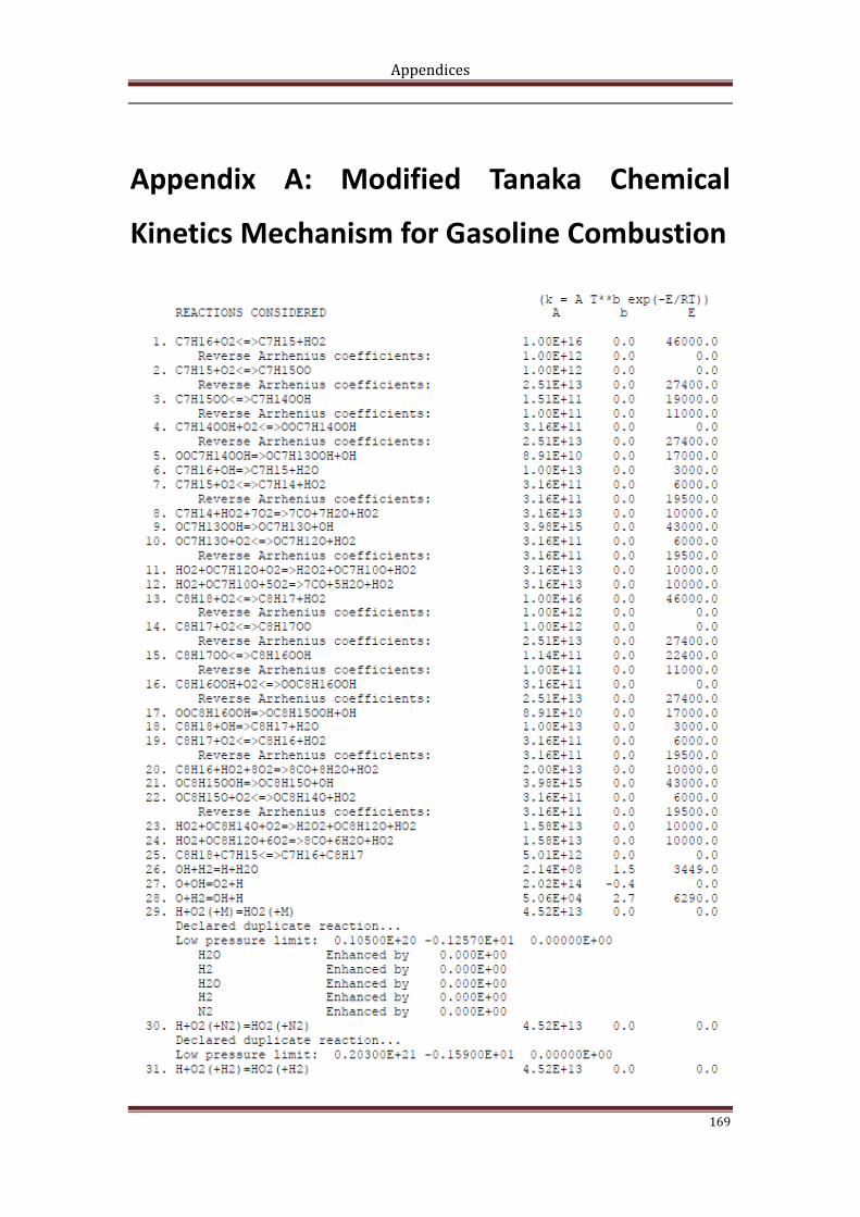
Appendices
169
Appendix A: Modified Tanaka Chemical
Kinetics Mechanism for Gasoline Combustion
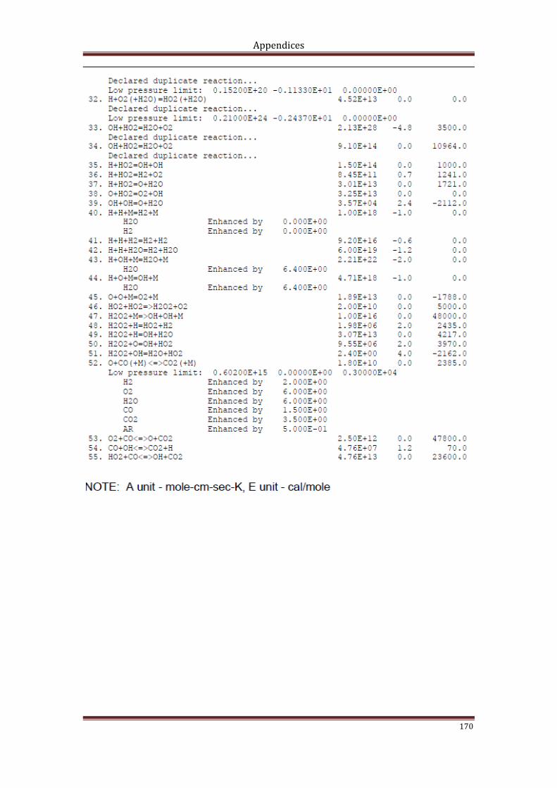
Appendices
170
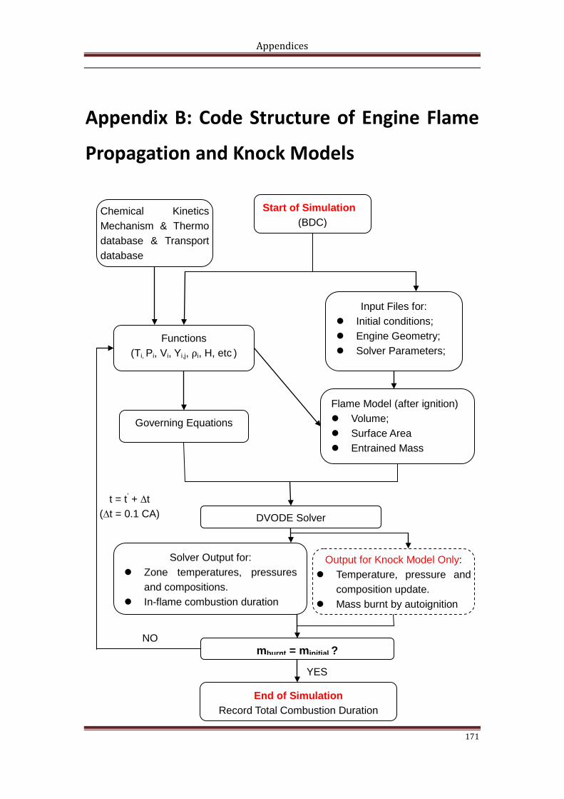
Appendices
171
Appendix B: Code Structure of Engine Flame
Propagation and Knock Models
Start of Simulation (BDC)
Chemical Kinetics Mechanism & Thermo database & Transport database
Functions (Ti, Pi, Vi, Yi,j, ρi, H, etc )
Input Files for: Initial conditions; Engine Geometry; Solver Parameters;
Flame Model (after ignition) Volume; Surface Area Entrained Mass
DVODE Solver
Governing Equations
Solver Output for: Zone temperatures, pressures
and compositions. In-flame combustion duration
mburnt = minitial ? NO
YES
Output for Knock Model Only: Temperature, pressure and
composition update. Mass burnt by autoignition
t = t’ + ∆t (∆t = 0.1 CA)
End of Simulation Record Total Combustion Duration
Recommended