Chapter8dp&c8-1
“Education in Pursuit of Supply Chain Leadership”
Chapter 8
Chapter8dp&c
Statistical Inventory Management

Chapter8dp&c8-2
• Understand the demand driver
• Define the concepts of stock replenishment
• Describe the replenishment review interval
• Review the basic terms of statistical inventory replenishment
• Review the basic inventory replenishment techniques
• Detail the basic of the reorder point
• Work with reorder point lead time and safety stock
• Explore min/max and periodic review methods
Learning Objectives
Chapter8dp&c8-3
• Define order quantity techniques
• Calculate the economic order quantity (EOQ)
• Detail the assumption of the EOQ technique
• Calculate order quantity discounts
• Perform order quantity joint replenishment
• Determine the transportation EOQ
• Discuss replenishment by item class
• Discuss the application of lean to statistical order management
Learning Objectives (cont.)
Chapter8dp&c8-4
Inventory Management Basics
Chapter 8Statistical Inventory Management
Statistical Inventory Replenishment
Concepts
Chapter8dp&c8-5
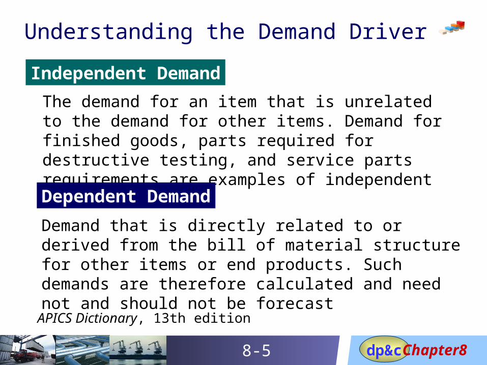
Understanding the Demand Driver
Independent Demand
The demand for an item that is unrelated to the demand for other items. Demand for finished goods, parts required for destructive testing, and service parts requirements are examples of independent demand
Dependent Demand
Demand that is directly related to or derived from the bill of material structure for other items or end products. Such demands are therefore calculated and need not and should not be forecast
APICS Dictionary, 13th edition
Chapter8dp&c8-6
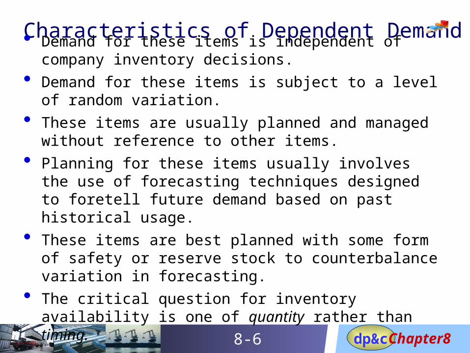
Characteristics of Dependent Demand
• Demand for these items is independent of company inventory decisions.
• Demand for these items is subject to a level of random variation.
• These items are usually planned and managed without reference to other items.
• Planning for these items usually involves the use of forecasting techniques designed to foretell future demand based on past historical usage.
• These items are best planned with some form of safety or reserve stock to counterbalance variation in forecasting.
• The critical question for inventory availability is one of quantity rather than timing.
Chapter8dp&c8-7
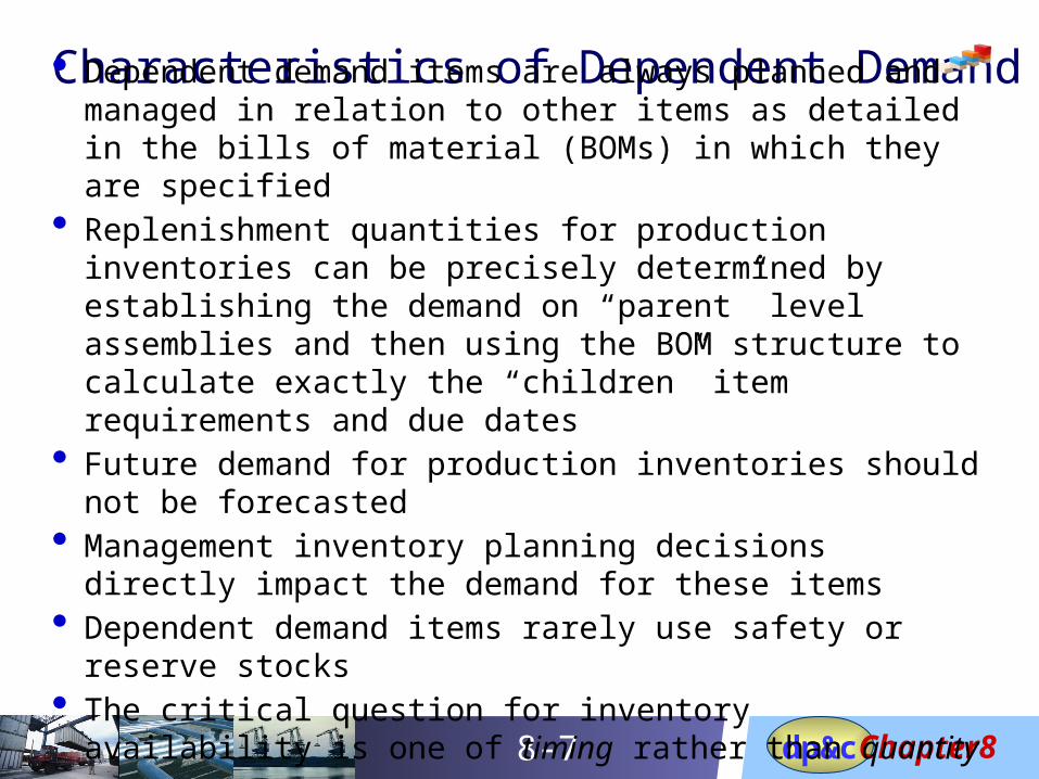
Characteristics of Dependent Demand
• Dependent demand items are always planned and managed in relation to other items as detailed in the bills of material (BOMs) in which they are specified
• Replenishment quantities for production inventories can be precisely determined by establishing the demand on “parent” level assemblies and then using the BOM structure to calculate exactly the “children” item requirements and due dates
• Future demand for production inventories should not be forecasted
• Management inventory planning decisions directly impact the demand for these items
• Dependent demand items rarely use safety or reserve stocks• The critical question for inventory availability is one of timing
rather than quantity
Chapter8dp&c8-8
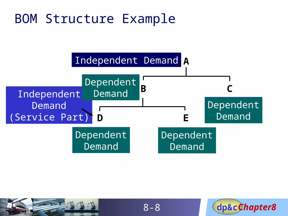
BOM Structure Example
A
B C
D E
Independent Demand
IndependentDemand
(Service Part)
DependentDemand
DependentDemand
DependentDemand
DependentDemand
Chapter8dp&c8-9
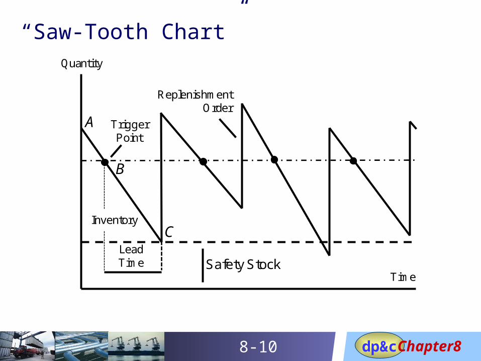
Concept of Inventory Replenishment
The theory behind inventory replenishment
management is that for each item, an optimal
stocking and ordering quantity can be determined
either statistically or through some form of
experience, or even intuition. The object is to
ensure that the optimum stocking level for each
item in the inventory is maintained at the targeted
service level without creating excess stock.
Chapter8dp&c8-10
“Saw-Tooth Chart”
A TriggerPoint
Safety Stock
Quantity
LeadTime
ReplenishmentOrder
Time
Inventory
B
C
Chapter8dp&c8-11
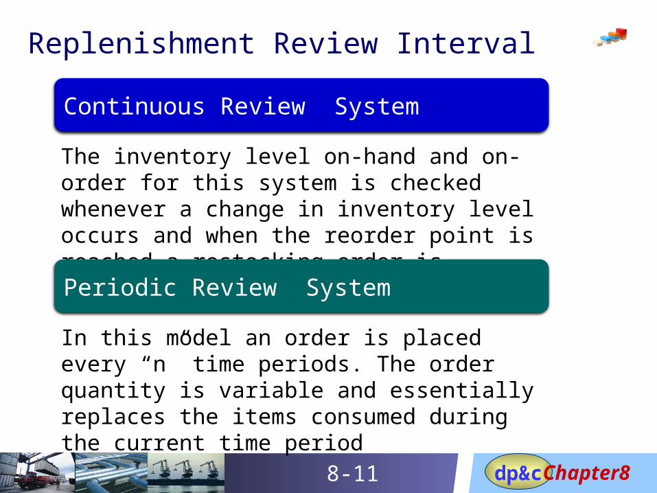
Replenishment Review Interval
Continuous Review System
The inventory level on-hand and on-order for this system is checked whenever a change in inventory level occurs and when the reorder point is reached a restocking order is released
Periodic Review System
In this model an order is placed every “n” time periods. The order quantity is variable and essentially replaces the items consumed during the current time period
Chapter8dp&c8-12
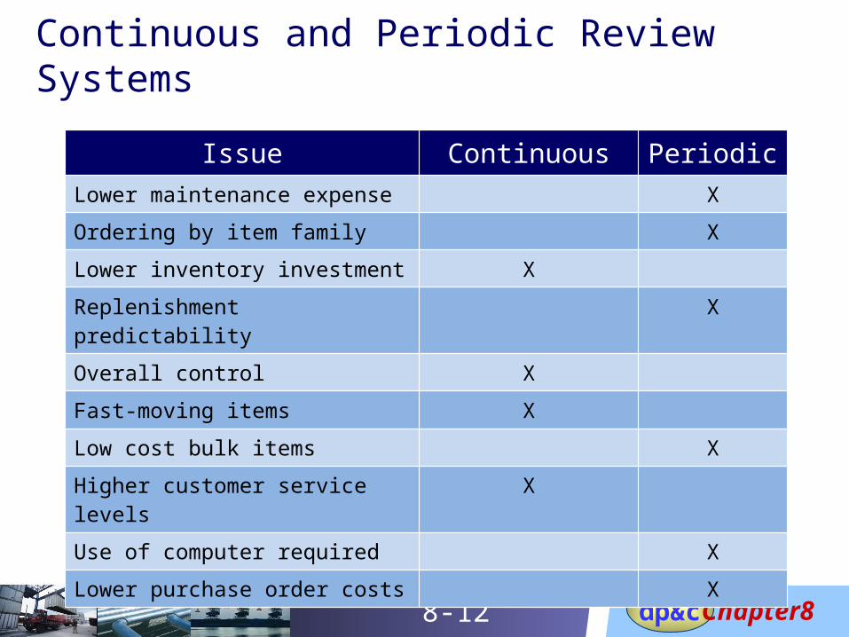
Continuous and Periodic Review Systems
Issue Continuous PeriodicLower maintenance expense X
Ordering by item family X
Lower inventory investment X
Replenishment predictability X
Overall control X
Fast-moving items X
Low cost bulk items X
Higher customer service levels X
Use of computer required X
Lower purchase order costs X
Chapter8dp&c8-13
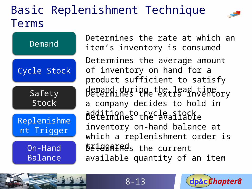
Demand
Cycle Stock
Safety Stock
Replenishment Trigger
On-Hand Balance
Determines the rate at which an item’s inventory is consumed
Determines the average amount of inventory on hand for a product sufficient to satisfy demand during the lead time
Determines the extra inventory a company decides to hold in addition to cycle stock
Determines the available inventory on-hand balance at which a replenishment order is triggered
Determines the current available quantity of an item
Basic Replenishment Technique Terms
Chapter8dp&c8-14
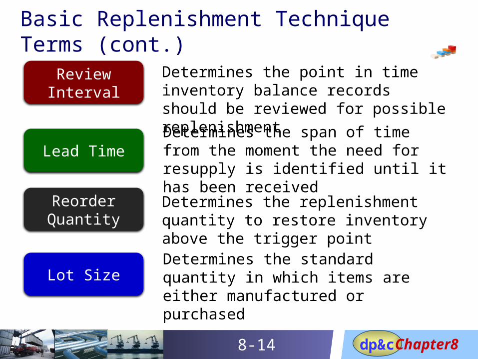
Review Interval
Lead Time
Reorder Quantity
Lot Size
Determines the point in time inventory balance records should be reviewed for possible replenishment
Determines the span of time from the moment the need for resupply is identified until it has been received
Determines the replenishment quantity to restore inventory above the trigger point
Determines the standard quantity in which items are either manufactured or purchased
Basic Replenishment Technique Terms (cont.)
Chapter8dp&c8-15
Inventory Management Basics
Chapter 8Statistical Inventory Management
InventoryReplenishment
Techniques
Chapter8dp&c8-16
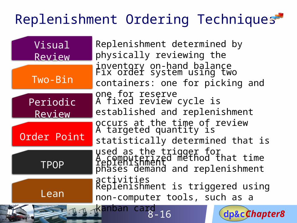
Replenishment Ordering Techniques
Visual Review
Two-Bin
Periodic Review
Order Point
TPOP
Lean
Replenishment determined by physically reviewing the inventory on-hand balance
Fix order system using two containers: one for picking and one for reserve
A fixed review cycle is established and replenishment occurs at the time of review
A targeted quantity is statistically determined that is used as the trigger for replenishment
A computerized method that time phases demand and replenishment activities
Replenishment is triggered using non-computer tools, such as a kanban card
Chapter8dp&c8-17
Inventory Management Basics
Chapter 8Statistical Inventory Management
Reorder Point Systems
Chapter8dp&c8-18
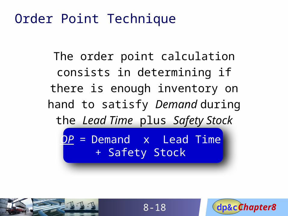
Order Point Technique
The order point calculation consists in
determining if there is enough
inventory on hand to satisfy Demand
during the Lead Time plus Safety Stock
OP = Demand x Lead Time + Safety Stock
Chapter8dp&c8-19
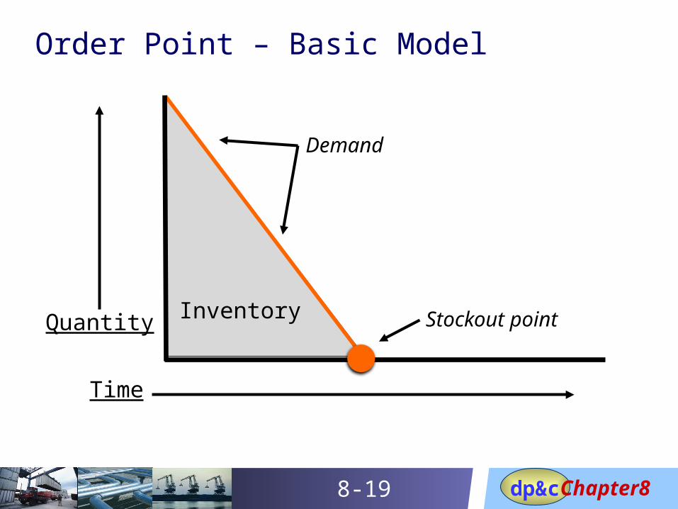
Order Point – Basic Model
Quantity
Time
Inventory
Demand
Stockout point
Chapter8dp&c8-20
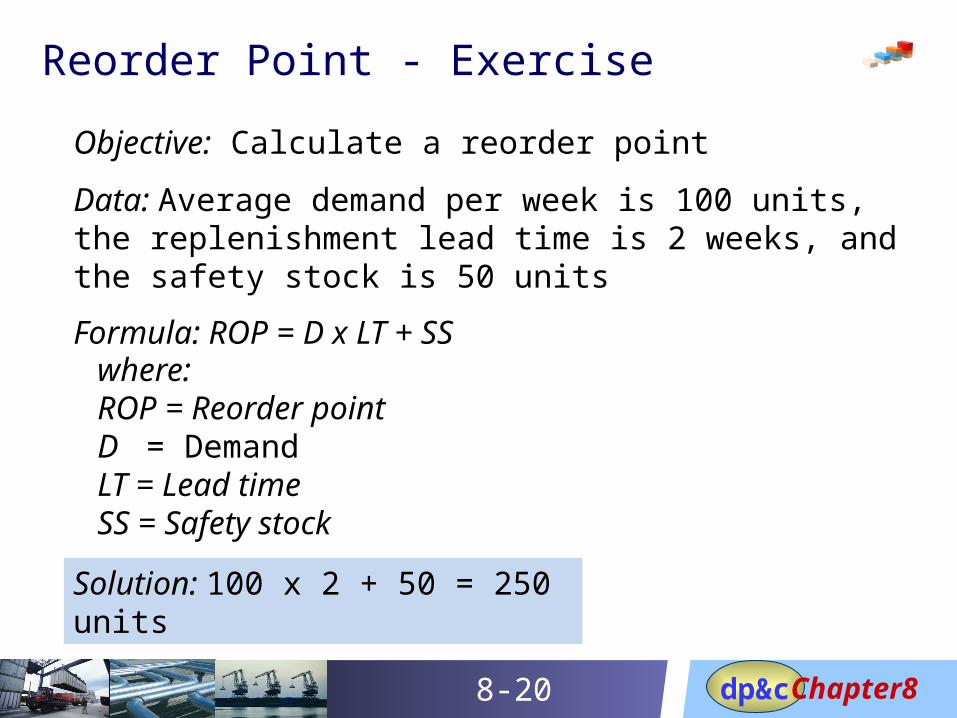
Reorder Point - Exercise
Objective: Calculate a reorder point
Data: Average demand per week is 100 units, the replenishment lead time is 2 weeks, and the safety stock is 50 units
Formula: ROP = D x LT + SS where: ROP = Reorder pointD = DemandLT = Lead timeSS = Safety stock
Solution: 100 x 2 + 50 = 250 units
Chapter8dp&c8-21
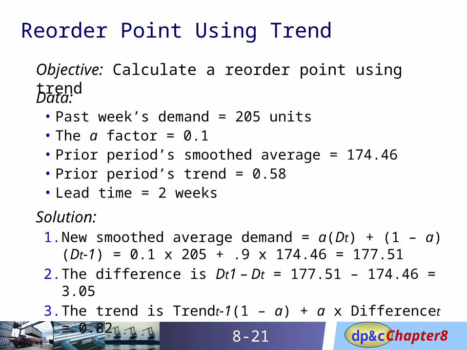
Reorder Point Using Trend
Objective: Calculate a reorder point using trend
Data: • Past week’s demand = 205 units• The a factor = 0.1• Prior period’s smoothed average = 174.46• Prior period’s trend = 0.58• Lead time = 2 weeks
Solution: 1. New smoothed average demand = a(Dt) + (1 – a) (Dt-1) =
0.1 x 205 + .9 x 174.46 = 177.512. The difference is Dt1 – Dt = 177.51 – 174.46 = 3.053. The trend is Trendt-1(1 – a) + a x Differencet = 0.82
Chapter8dp&c8-22
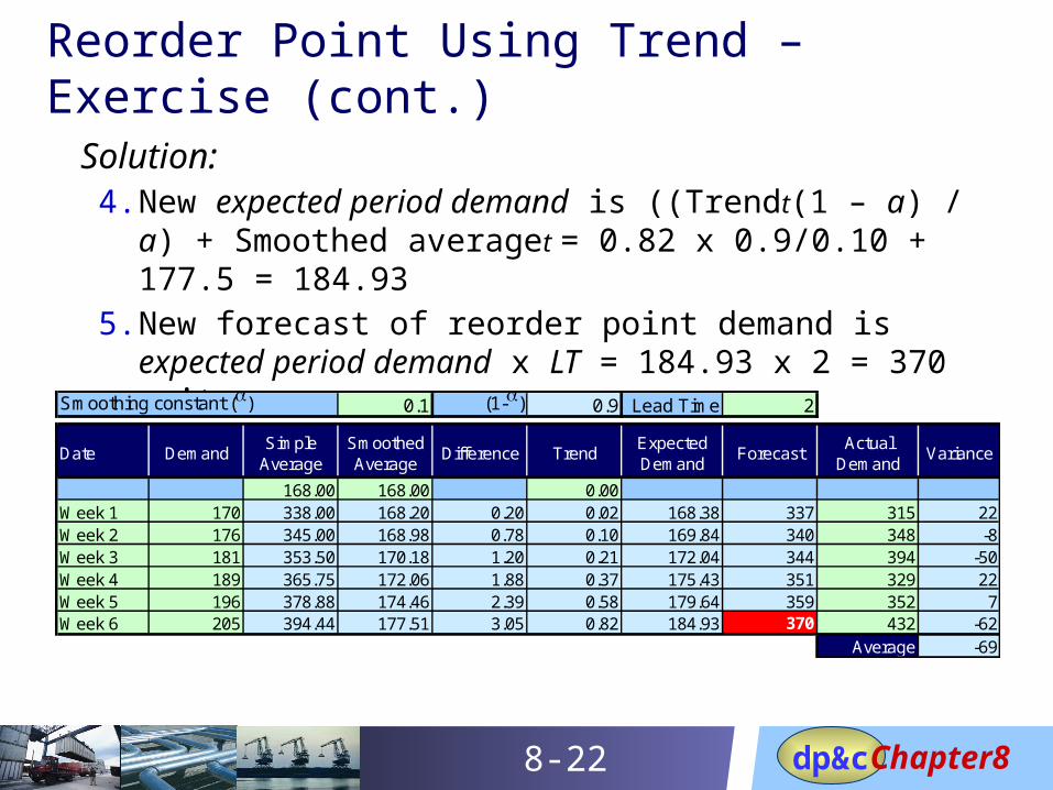
Reorder Point Using Trend – Exercise (cont.)
Solution: 4. New expected period demand is ((Trendt(1 – a) / a) +
Smoothed averaget = 0.82 x 0.9/0.10 + 177.5 = 184.935. New forecast of reorder point demand is expected period
demand x LT = 184.93 x 2 = 370 units
Smoothing constant (a) 0.1 (1-a) 0.9 Lead Time 2
Date DemandSimple
AverageSmoothed Average
Difference TrendExpected Demand
Forecast Actual
DemandVariance
168.00 168.00 0.00Week 1 170 338.00 168.20 0.20 0.02 168.38 337 315 22Week 2 176 345.00 168.98 0.78 0.10 169.84 340 348 -8Week 3 181 353.50 170.18 1.20 0.21 172.04 344 394 -50Week 4 189 365.75 172.06 1.88 0.37 175.43 351 329 22Week 5 196 378.88 174.46 2.39 0.58 179.64 359 352 7Week 6 205 394.44 177.51 3.05 0.82 184.93 370 432 -62
Average -69
Chapter8dp&c8-23
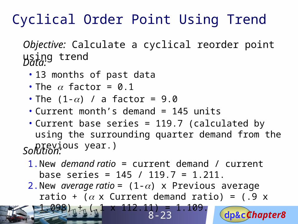
Cyclical Order Point Using Trend
Objective: Calculate a cyclical reorder point using trend
Data: • 13 months of past data• The a factor = 0.1• The (1-a) / a factor = 9.0• Current month’s demand = 145 units• Current base series = 119.7 (calculated by using the
surrounding quarter demand from the previous year.)
Solution: 1. New demand ratio = current demand / current base series =
145 / 119.7 = 1.211.2. New average ratio = (1-a) x Previous average ratio + ( a x
Current demand ratio) = (.9 x 1.098) + (.1 x 112.11) = 1.109.
Chapter8dp&c8-24
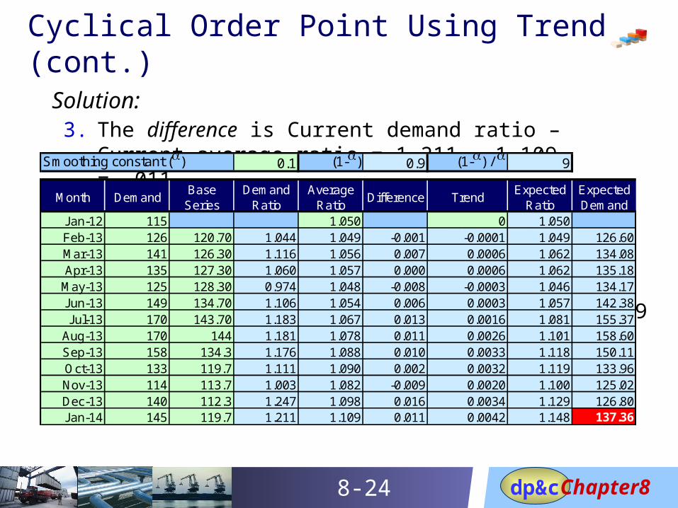
Cyclical Order Point Using Trend (cont.)
Solution: 3. The difference is Current demand ratio – Current average
ratio = 1.211 – 1.109 = .011.4. New trend is (1-a) x Previous trend + (a x Current difference)
= (.9 x .0034) + (.1 x .011) = .0042.5. New expected ratio is Current period average ratio + (1-a) / a
+ Current trend = 1.109 + 9 + .0042 = 1.148.6. New expected demand is Current expected ratio x current
base series = 1.148 x 119.7 = 137.36
Smoothing constant (a) 0.1 (1-a) 0.9 (1-a) / a 9
Month DemandBase
SeriesDemand
RatioAverage
RatioDifference Trend
Expected Ratio
Expected Demand
Jan-12 115 1.050 0 1.050Feb-13 126 120.70 1.044 1.049 -0.001 -0.0001 1.049 126.60Mar-13 141 126.30 1.116 1.056 0.007 0.0006 1.062 134.08Apr-13 135 127.30 1.060 1.057 0.000 0.0006 1.062 135.18
May-13 125 128.30 0.974 1.048 -0.008 -0.0003 1.046 134.17Jun-13 149 134.70 1.106 1.054 0.006 0.0003 1.057 142.38Jul-13 170 143.70 1.183 1.067 0.013 0.0016 1.081 155.37
Aug-13 170 144 1.181 1.078 0.011 0.0026 1.101 158.60Sep-13 158 134.3 1.176 1.088 0.010 0.0033 1.118 150.11Oct-13 133 119.7 1.111 1.090 0.002 0.0032 1.119 133.96Nov-13 114 113.7 1.003 1.082 -0.009 0.0020 1.100 125.02Dec-13 140 112.3 1.247 1.098 0.016 0.0034 1.129 126.80Jan-14 145 119.7 1.211 1.109 0.011 0.0042 1.148 137.36
Chapter8dp&c8-25
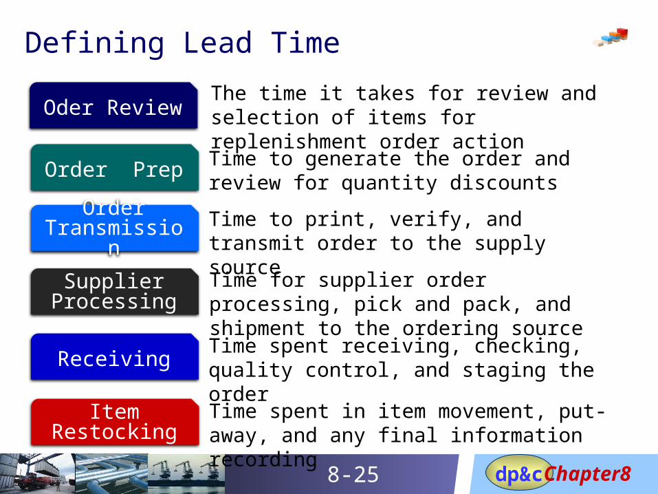
Defining Lead Time
Oder ReviewThe time it takes for review and selection of items for replenishment order action
Order Prep Time to generate the order and review for quantity discounts
Order Transmission
Time to print, verify, and transmit order to the supply source
Supplier Processing
Time for supplier order processing, pick and pack, and shipment to the ordering source
ReceivingTime spent receiving, checking, quality control, and staging the order
Item Restocking
Time spent in item movement, put-away, and any final information recording
Chapter8dp&c8-26
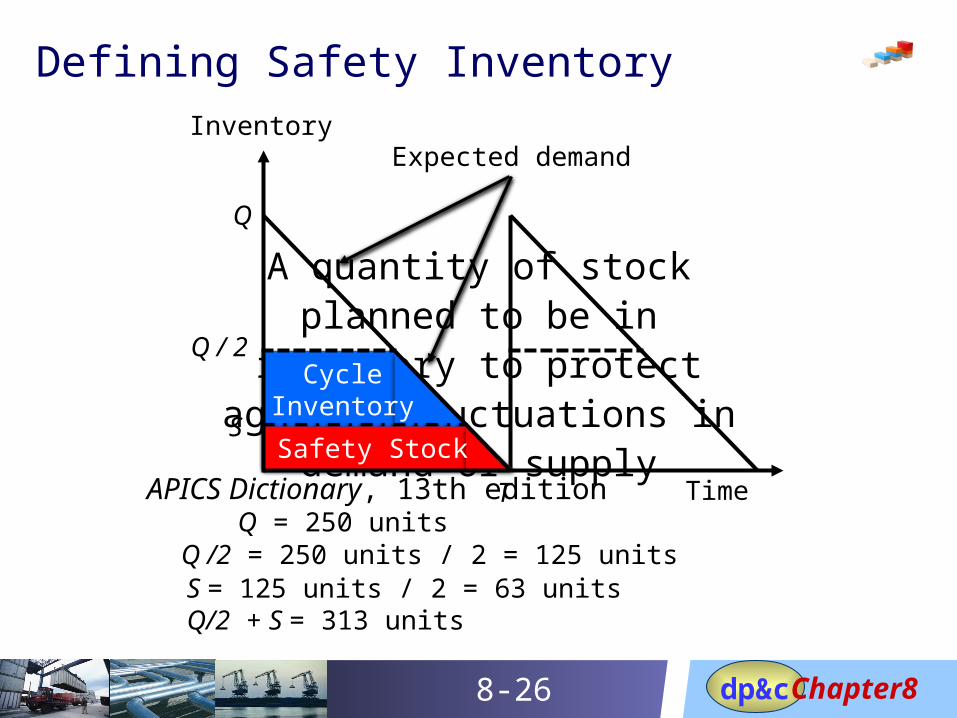
Defining Safety Inventory
A quantity of stock planned to be in inventory to protect against
fluctuations in demand or supply
APICS Dictionary, 13th edition
Q /2 = 250 units / 2 = 125 unitsS = 125 units / 2 = 63 unitsQ/2 + S = 313 units
Inventory
Q
T Time
Expected demand
Q / 2Cycle
Inventory
Safety StockS
Q = 250 units
Chapter8dp&c8-27
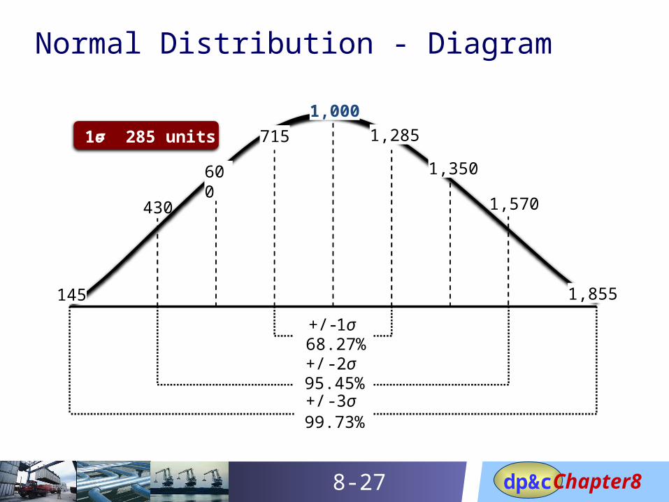
Normal Distribution - Diagram
430 1,570
+/ -1σ68.27%+/ - 2σ95.45%
1σ = 285 units
+/ - 3σ99.73%
1,0001,285715
1,350600
1,855145
Chapter8dp&c8-28
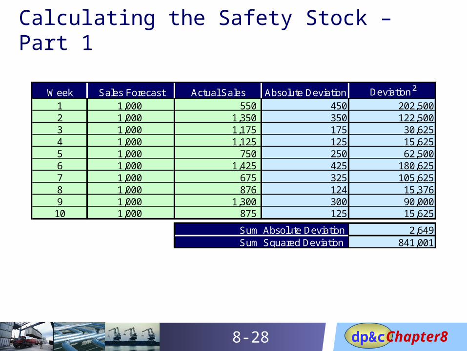
Calculating the Safety Stock – Part 1
Week Sales Forecast Actual Sales Absolute Deviation Deviation²1 1,000 550 450 202,5002 1,000 1,350 350 122,5003 1,000 1,175 175 30,6254 1,000 1,125 125 15,6255 1,000 750 250 62,5006 1,000 1,425 425 180,6257 1,000 675 325 105,6258 1,000 876 124 15,3769 1,000 1,300 300 90,000
10 1,000 875 125 15,625
Sum Absolute Deviation 2,649Sum Squared Deviation 841,001
Chapter8dp&c8-29
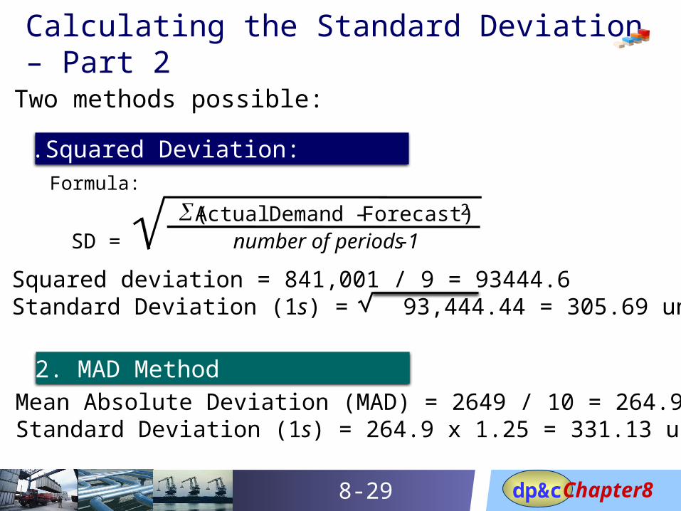
Calculating the Standard Deviation – Part 2
a.) Mean Absolute Deviation (MAD) = 2649 / 10 = 264.9b.) Standard Deviation (1s) = 264.9 x 1.25 = 331.13 units
Two methods possible:
a.) Squared deviation = 841,001 / 9 = 93444.6b.) Standard Deviation (1s) = 93,444.44 = 305.69 units
Formula:
1. Squared Deviation:
2. MAD Method
å (Actual Demand – Forecast)2
SD = number of periods-1
Chapter8dp&c8-30
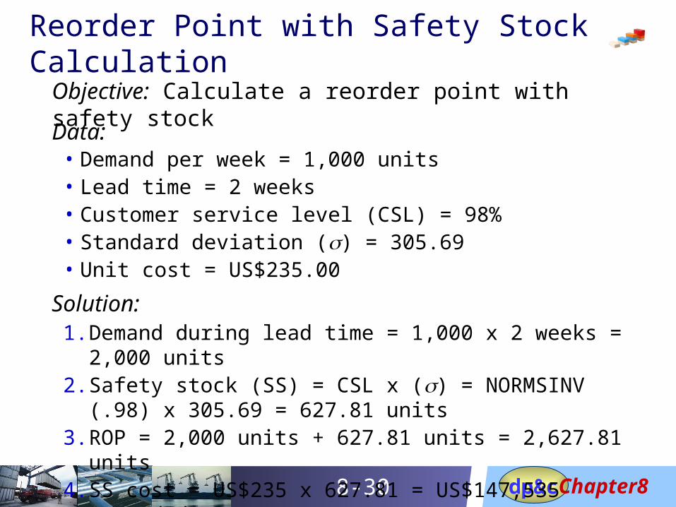
Reorder Point with Safety Stock Calculation
Objective: Calculate a reorder point with safety stock
Data: • Demand per week = 1,000 units• Lead time = 2 weeks• Customer service level (CSL) = 98%• Standard deviation (s) = 305.69• Unit cost = US$235.00
Solution: 1. Demand during lead time = 1,000 x 2 weeks = 2,000 units2. Safety stock (SS) = CSL x (s) = NORMSINV (.98) x 305.69 =
627.81 units3. ROP = 2,000 units + 627.81 units = 2,627.81 units4. SS cost = US$235 x 627.81 = US$147,535 (rounded)
Chapter8dp&c8-31
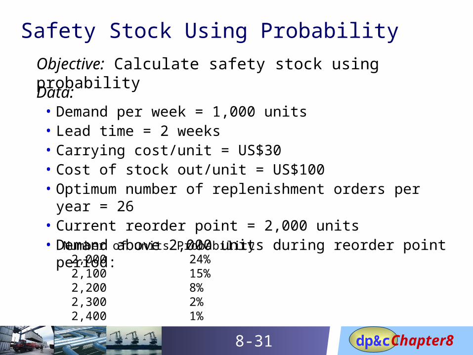
Safety Stock Using Probability
Objective: Calculate safety stock using probability
Data: • Demand per week = 1,000 units• Lead time = 2 weeks• Carrying cost/unit = US$30• Cost of stock out/unit = US$100• Optimum number of replenishment orders per year = 26• Current reorder point = 2,000 units• Demand above 2,000 units during reorder point period:
Number of units2,0002,1002,2002,3002,400
Probability24%15%8%2%1%
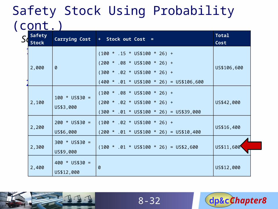
Chapter8dp&c8-32
Solution: 1. Calculate safety stock carrying cost by multiplying the
carrying cost times the safety stock2. Calculate stock out cost: the sum of the units stocked out x
the probability x the unit cost x the number of orders per year
Safety Stock Using Probability (cont.)SafetyStock
Carrying Cost + Stock out Cost = TotalCost
2,000 0
(100 * .15 * US$100 * 26) +
(200 * .08 * US$100 * 26) +
(300 * .02 * US$100 * 26) +
(400 * .01 * US$100 * 26) = US$106,600
US$106,600
2,100100 * US$30 =
US$3,000
(100 * .08 * US$100 * 26) +
(200 * .02 * US$100 * 26) +
(300 * .01 * US$100 * 26) = US$39,000
US$42,000
2,200200 * US$30 =
US$6,000
(100 * .02 * US$100 * 26) +
(200 * .01 * US$100 * 26) = US$10,400US$16,400
2,300300 * US$30 =
US$9,000(100 * .01 * US$100 * 26) = US$2,600 US$11,600
2,400400 * US$30 =
US$12,0000 US$12,000
Chapter8dp&c8-33
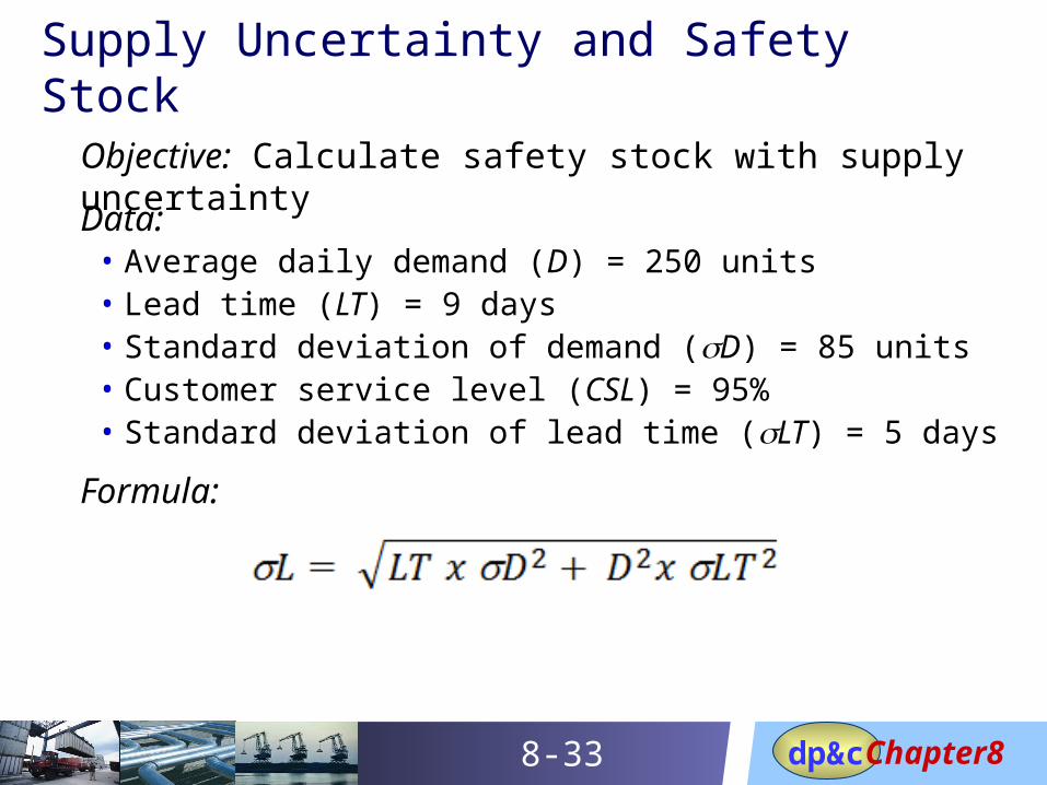
Supply Uncertainty and Safety Stock
Objective: Calculate safety stock with supply uncertainty
Data: • Average daily demand (D) = 250 units• Lead time (LT) = 9 days• Standard deviation of demand (sD) = 85 units• Customer service level (CSL) = 95%• Standard deviation of lead time (sLT) = 5 days
Formula:
Chapter8dp&c8-34
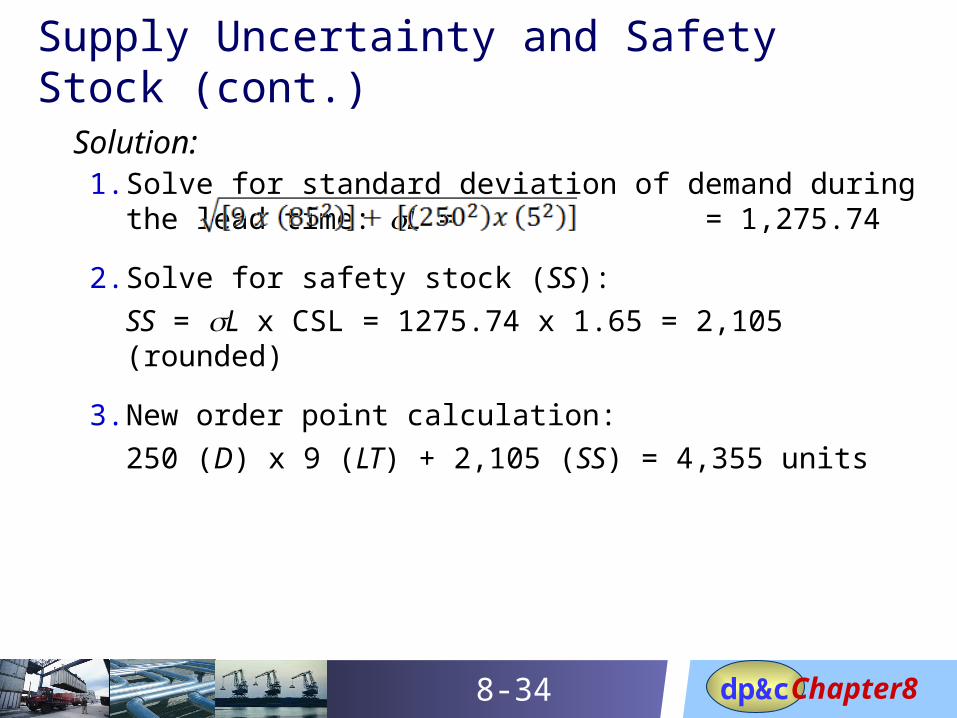
Supply Uncertainty and Safety Stock (cont.)
Solution: 1. Solve for standard deviation of demand during the lead time:
sL = = 1,275.74
2. Solve for safety stock (SS):
SS = sL x CSL = 1275.74 x 1.65 = 2,105 (rounded)
3. New order point calculation:
250 (D) x 9 (LT) + 2,105 (SS) = 4,355 units
Chapter8dp&c8-35
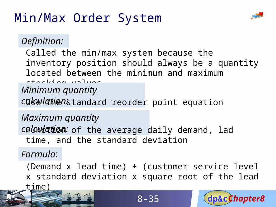
Min/Max Order System
Definition:Called the min/max system because the inventory position should always be a quantity located between the minimum and maximum stocking values
Minimum quantity calculation: Use the standard reorder point equation
Maximum quantity calculation: Function of the average daily demand, lad time, and the standard deviation
Formula: (Demand x lead time) + (customer service level x standard deviation x square root of the lead time)
Chapter8dp&c8-36
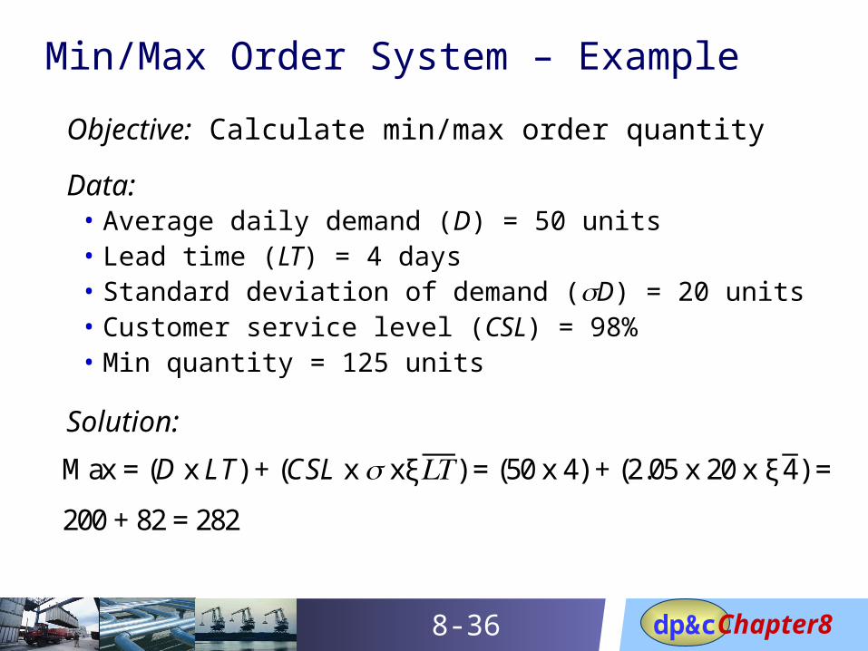
Min/Max Order System – Example
Objective: Calculate min/max order quantity
Data: • Average daily demand (D) = 50 units• Lead time (LT) = 4 days• Standard deviation of demand (sD) = 20 units• Customer service level (CSL) = 98%• Min quantity = 125 units
Solution:
Max = (D x LT) + (CSL x xξ𝐿𝑇) = (50 x 4) + (2.05 x 20 x ξ4) =
200 + 82 = 282
Chapter8dp&c8-37
Periodic Review – Overview
Definition:Items are reviewed periodically and replenishment orders are launched at each review. The order quantity contains sufficient stock to bring the inventory position up to a target inventory level
Uses:
1. Used when it is difficult to record withdrawals and additions of stock on a continuous basis
2. Used when items are ordered in families
3. Used for items with a limited shelf life
4. Significant economies can be gained by ordering in bulk
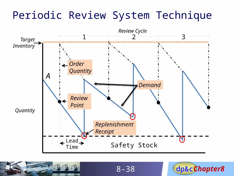
Chapter8dp&c8-38
Periodic Review System Technique
A
Safety Stock
Review Cycle321
LeadTime
OrderQuantity
Demand
ReviewPoint
ReplenishmentReceipt
TargetInventory
Quantity
Chapter8dp&c8-39
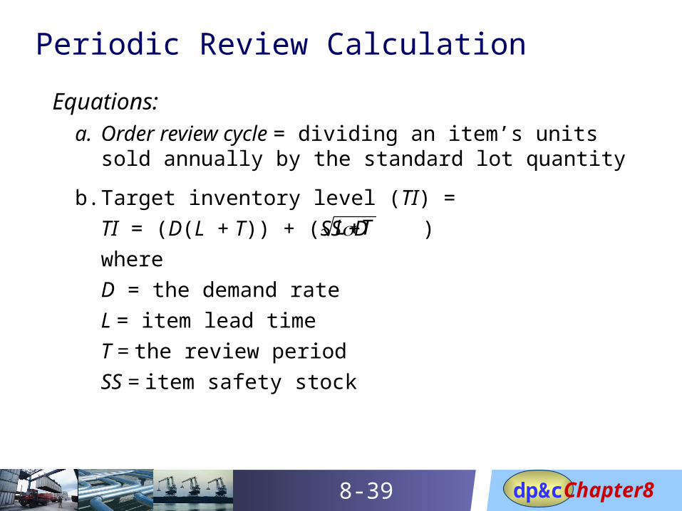
Periodic Review Calculation
Equations: a. Order review cycle = dividing an item’s units sold annually
by the standard lot quantity
b. Target inventory level (TI) =
TI = (D(L + T)) + (SSsD )
where
D = the demand rate
L = item lead time
T = the review period
SS = item safety stock
TL
Chapter8dp&c8-40
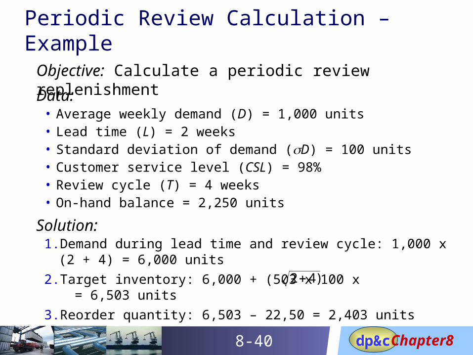
Periodic Review Calculation – Example
Objective: Calculate a periodic review replenishment
Data: • Average weekly demand (D) = 1,000 units• Lead time (L) = 2 weeks• Standard deviation of demand (sD) = 100 units• Customer service level (CSL) = 98%• Review cycle (T) = 4 weeks• On-hand balance = 2,250 units
Solution: 1. Demand during lead time and review cycle: 1,000 x (2 + 4) = 6,000
units
2. Target inventory: 6,000 + (503 x 100 x = 6,503 units
3. Reorder quantity: 6,503 – 22,50 = 2,403 units
)42
Chapter8dp&c8-41
Inventory Management Basics
Chapter 8Statistical Inventory Management
Order Quantity Techniques
Chapter8dp&c8-42
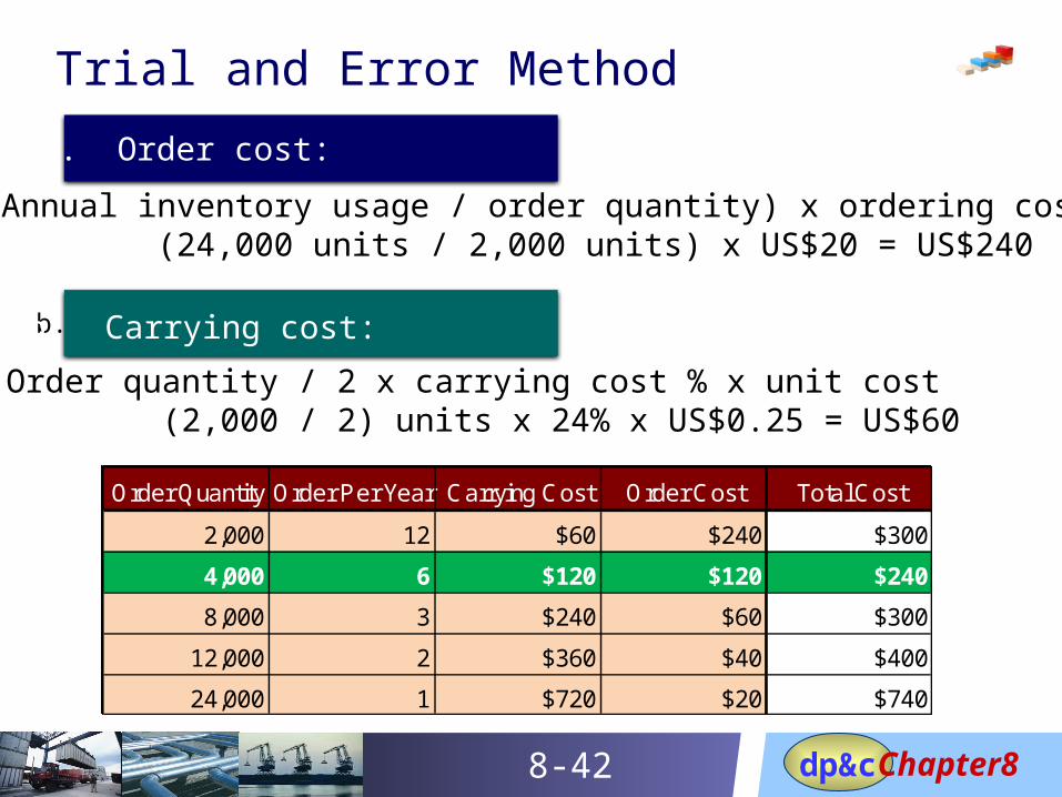
Trial and Error Method
(Annual inventory usage / order quantity) x ordering cost (24,000 units / 2,000 units) x US$20 = US$240
b. Carrying cost:
Order quantity / 2 x carrying cost % x unit cost (2,000 / 2) units x 24% x US$0.25 = US$60
b. Carrying cost:
a. Order cost:
Order Quantity Order Per Year Carrying Cost Order Cost Total Cost
2,000 12 $60 $240
4,000 6 $120 $120
8,000 3 $240 $60
12,000 2 $360 $40
24,000 1 $720 $20
Order Quantity Order Per Year Carrying Cost Order Cost Total Cost
2,000 12 $60 $240 $300
4,000 6 $120 $120 $240
8,000 3 $240 $60 $300
12,000 2 $360 $40 $400
24,000 1 $720 $20 $740
Chapter8dp&c8-43
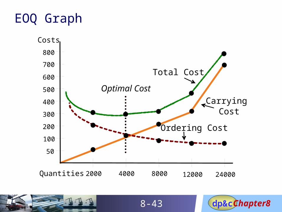
EOQ Graph
50
100
200
300
400
2000 4000 12000 24000
500
600
700
800
Optimal Cost
Total Cost
CarryingCost
Ordering Cost
Costs
Quantities 8000
Chapter8dp&c8-44
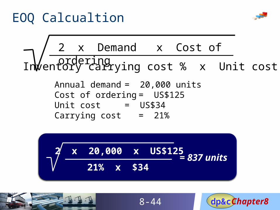
EOQ Calcualtion
2 x Demand x Cost of ordering
Inventory carrying cost % x Unit cost
Annual demand = 20,000 unitsCost of ordering = US$125Unit cost = US$34Carrying cost = 21%
2 x 20,000 x US$125
21% x $34= 837 units
Chapter8dp&c8-45
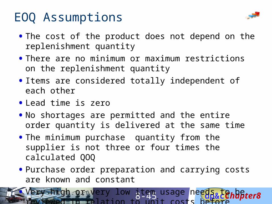
EOQ Assumptions
• The cost of the product does not depend on the replenishment quantity
• There are no minimum or maximum restrictions on the replenishment quantity
• Items are considered totally independent of each other
• Lead time is zero
• No shortages are permitted and the entire order quantity is delivered at the same time
• The minimum purchase quantity from the supplier is not three or four times the calculated QOQ
• Purchase order preparation and carrying costs are known and constant
• Very high or very low item usage needs to be reviewed in relation to unit costs before applying the EOQ technique
Chapter8dp&c8-46
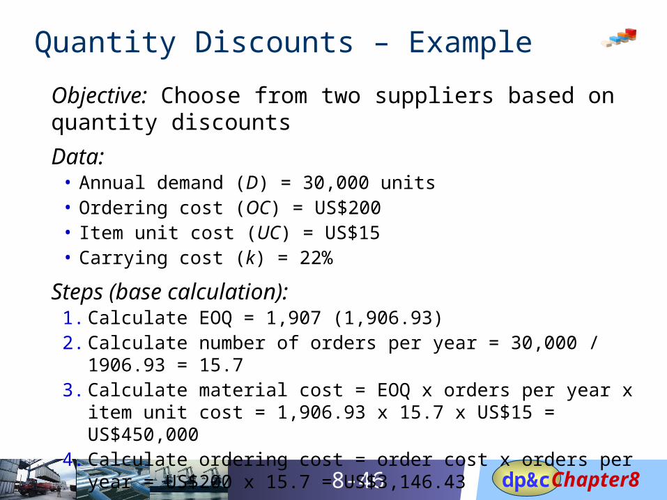
Quantity Discounts – Example
Objective: Choose from two suppliers based on quantity discounts
Data: • Annual demand (D) = 30,000 units• Ordering cost (OC) = US$200• Item unit cost (UC) = US$15• Carrying cost (k) = 22%
Steps (base calculation): 1. Calculate EOQ = 1,907 (1,906.93)2. Calculate number of orders per year = 30,000 / 1906.93 = 15.73. Calculate material cost = EOQ x orders per year x item unit cost =
1,906.93 x 15.7 x US$15 = US$450,0004. Calculate ordering cost = order cost x orders per year = US$200 x
15.7 = US$3,146.43
Chapter8dp&c8-47
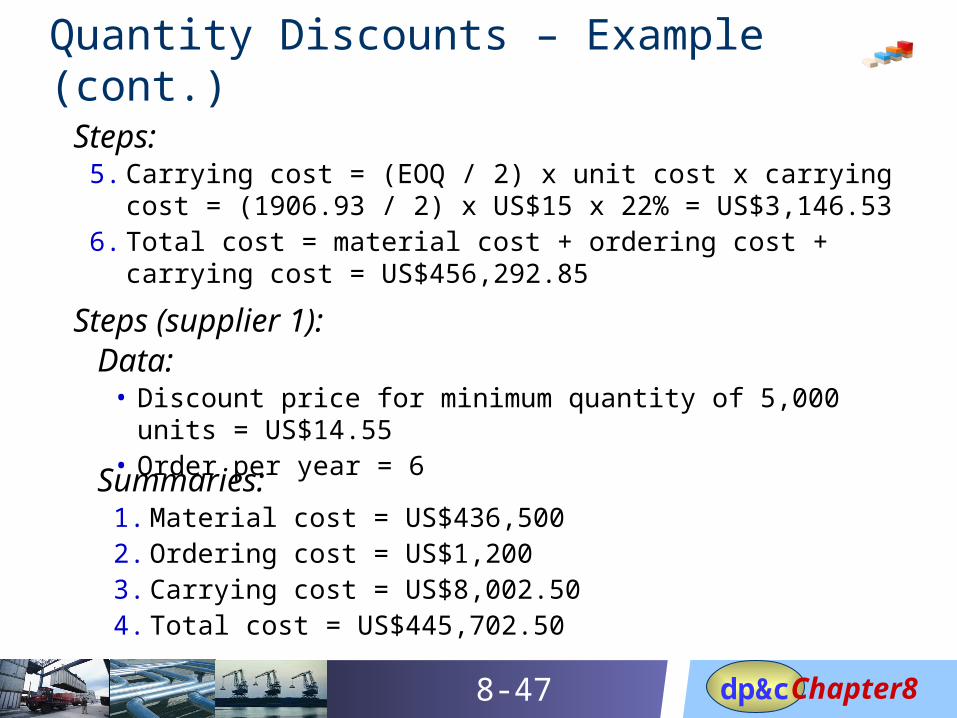
Quantity Discounts – Example (cont.)
Steps: 5. Carrying cost = (EOQ / 2) x unit cost x carrying cost = (1906.93 / 2)
x US$15 x 22% = US$3,146.536. Total cost = material cost + ordering cost + carrying cost =
US$456,292.85
Steps (supplier 1): Data:
• Discount price for minimum quantity of 5,000 units = US$14.55• Order per year = 6
Summaries: 1. Material cost = US$436,5002. Ordering cost = US$1,2003. Carrying cost = US$8,002.504. Total cost = US$445,702.50
Chapter8dp&c8-48
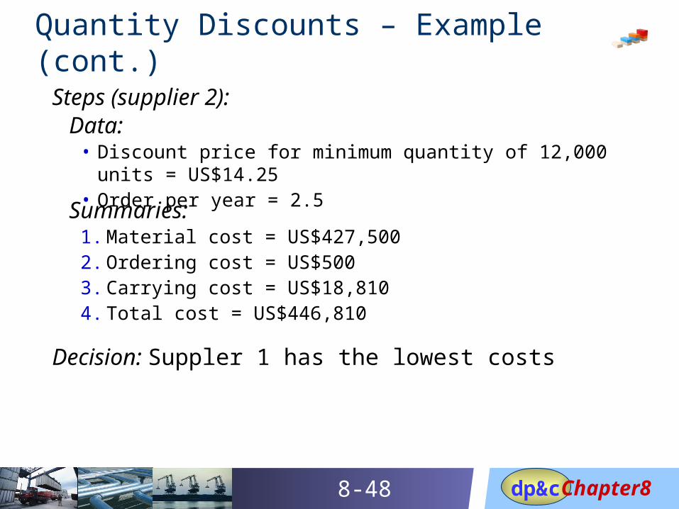
Quantity Discounts – Example (cont.)
Steps (supplier 2): Data:
• Discount price for minimum quantity of 12,000 units = US$14.25• Order per year = 2.5
Summaries: 1. Material cost = US$427,5002. Ordering cost = US$5003. Carrying cost = US$18,8104. Total cost = US$446,810
Decision: Suppler 1 has the lowest costs
Chapter8dp&c8-49
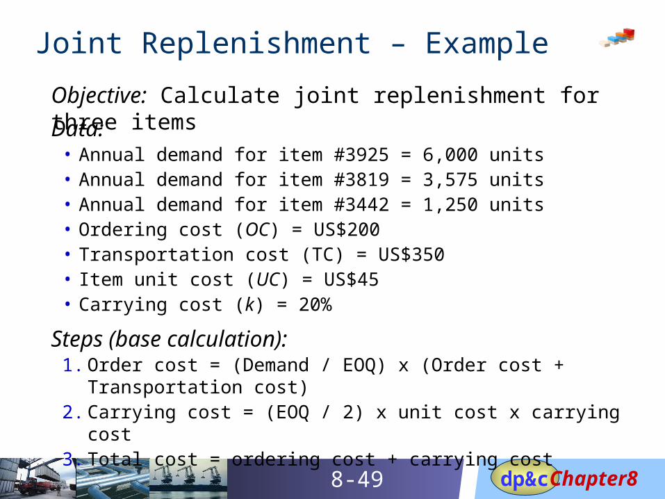
Joint Replenishment – Example
Objective: Calculate joint replenishment for three items
Data: • Annual demand for item #3925 = 6,000 units• Annual demand for item #3819 = 3,575 units• Annual demand for item #3442 = 1,250 units• Ordering cost (OC) = US$200• Transportation cost (TC) = US$350• Item unit cost (UC) = US$45• Carrying cost (k) = 20%
Steps (base calculation): 1. Order cost = (Demand / EOQ) x (Order cost + Transportation cost)2. Carrying cost = (EOQ / 2) x unit cost x carrying cost3. Total cost = ordering cost + carrying cost
Chapter8dp&c8-50
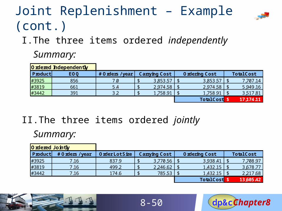
Joint Replenishment – Example (cont.)
I. The three items ordered independently
Summary: Ordered IndependentlyProduct EOQ # Orders / year Carrying Cost Ordering Cost Total Cost
#3925 856 7.0 3,853.57$ 3,853.57$ 7,707.14$ #3819 661 5.4 2,974.58$ 2,974.58$ 5,949.16$ #3442 391 3.2 1,758.91$ 1,758.91$ 3,517.81$
Total Cost 17,174.11$
II. The three items ordered jointly
Summary: Ordered JointlyProduct # Orders / year Order Lot Size Carrying Cost Ordering Cost Total Cost
#3925 7.16 837.9 3,770.56$ 3,938.41$ 7,708.97$ #3819 7.16 499.2 2,246.62$ 1,432.15$ 3,678.77$ #3442 7.16 174.6 785.53$ 1,432.15$ 2,217.68$
Total Cost 13,605.42$
Chapter8dp&c8-51
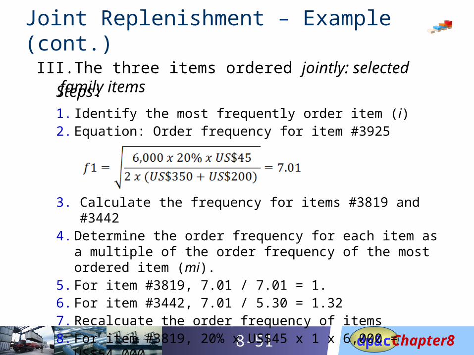
Joint Replenishment – Example (cont.)
III. The three items ordered jointly: selected family items
Steps:1. Identify the most frequently order item (i)2. Equation: Order frequency for item #3925
3. Calculate the frequency for items #3819 and #34424. Determine the order frequency for each item as a multiple of
the order frequency of the most ordered item (mi). 5. For item #3819, 7.01 / 7.01 = 1. 6. For item #3442, 7.01 / 5.30 = 1.327. Recalcuate the order frequency of items8. For item #3819, 20% x US$45 x 1 x 6,000 = US$54,000.
Chapter8dp&c8-52
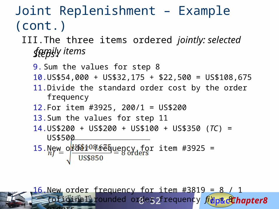
Joint Replenishment – Example (cont.)
III. The three items ordered jointly: selected family items
Steps:9. Sum the values for step 810. US$54,000 + US$32,175 + $22,500 = US$108,67511. Divide the standard order cost by the order frequency12. For item #3925, 200/1 = US$20013. Sum the values for step 1114. US$200 + US$200 + US$100 + US$350 (TC) = US$50015. New order frequency for item #3925 =
16. New order frequency for item #3819 = 8 / 1 (original rounded order frequency fi) = 8 orders.
Chapter8dp&c8-53
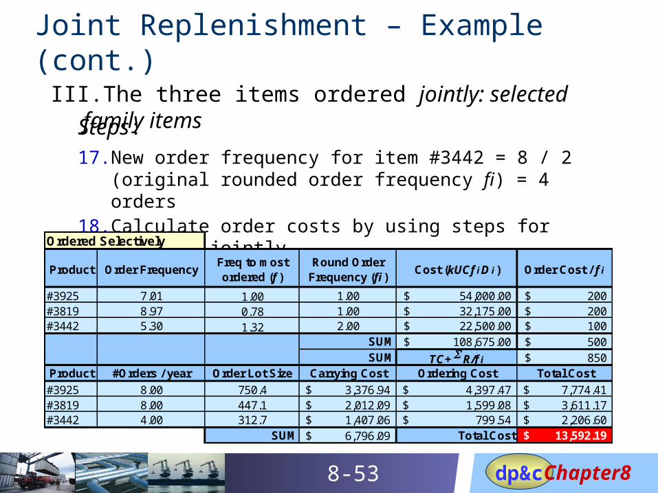
Joint Replenishment – Example (cont.)
III. The three items ordered jointly: selected family items
Steps:17. New order frequency for item #3442 = 8 / 2 (original rounded
order frequency fi) = 4 orders18. Calculate order costs by using steps for ordering jointly
Ordered Selectively
Product Order FrequencyFreq to most ordered (f )
Round Order Frequency (fi )
Cost (kUCf i D i ) Order Cost / f i
#3925 7.01 1.00 1.00 54,000.00$ 200$ #3819 8.97 0.78 1.00 32,175.00$ 200$ #3442 5.30 1.32 2.00 22,500.00$ 100$
SUM 108,675.00$ 500$ SUM TC+ S R/f i 850$
Product #Orders / year Order Lot Size Carrying Cost Ordering Cost Total Cost
#3925 8.00 750.4 3,376.94$ 4,397.47$ 7,774.41$ #3819 8.00 447.1 2,012.09$ 1,599.08$ 3,611.17$ #3442 4.00 312.7 1,407.06$ 799.54$ 2,206.60$
SUM 6,796.09$ Total Cost 13,592.19$
Chapter8dp&c8-54
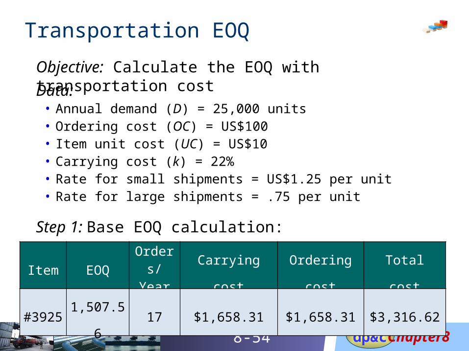
Transportation EOQ
Objective: Calculate the EOQ with transportation cost
Data: • Annual demand (D) = 25,000 units• Ordering cost (OC) = US$100• Item unit cost (UC) = US$10• Carrying cost (k) = 22%• Rate for small shipments = US$1.25 per unit• Rate for large shipments = .75 per unit
Step 1: Base EOQ calculation:
Item EOQOrders/
Year Carrying cost Ordering cost Total cost
#3925 1,507.56 17 $1,658.31 $1,658.31 $3,316.62
Chapter8dp&c8-55
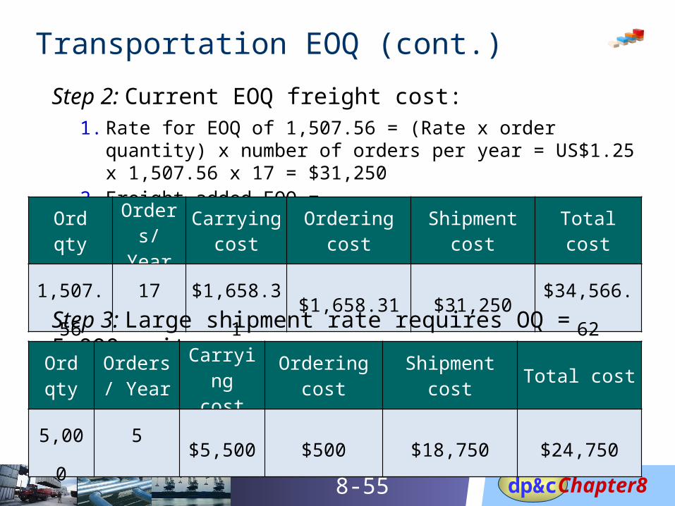
Transportation EOQ (cont.)
Step 2: Current EOQ freight cost: 1. Rate for EOQ of 1,507.56 = (Rate x order quantity) x number of
orders per year = US$1.25 x 1,507.56 x 17 = $31,2502. Freight added EOQ =
Ord qtyOrders/
YearCarrying
cost Ordering costShipment
cost Total cost
1,507.56 17 $1,658.31 $1,658.31 $31,250 $34,566.62
Step 3: Large shipment rate requires OQ = 5,000 units
Ord qty
Orders/ Year
Carrying cost
Ordering cost Shipment cost Total cost
5,000 5 $5,500 $500 $18,750 $24,750
Chapter8dp&c8-56
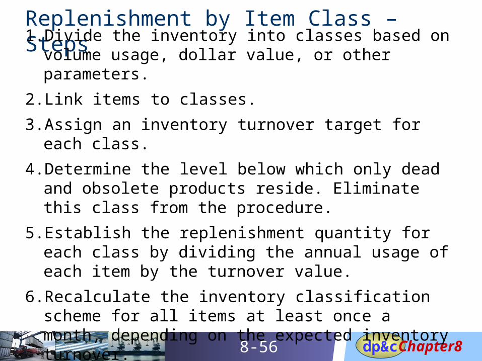
Replenishment by Item Class – Steps
1. Divide the inventory into classes based on volume usage, dollar value, or other parameters.
2. Link items to classes.
3. Assign an inventory turnover target for each class.
4. Determine the level below which only dead and obsolete products reside. Eliminate this class from the procedure.
5. Establish the replenishment quantity for each class by dividing the annual usage of each item by the turnover value.
6. Recalculate the inventory classification scheme for all items at least once a month, depending on the expected inventory turnover.
Chapter8dp&c8-57
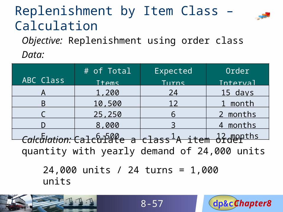
Replenishment by Item Class – Calculation
Objective: Replenishment using order class
Data:
ABC Class # of Total Items Expected Turns Order IntervalA 1,200 24 15 daysB 10,500 12 1 monthC 25,250 6 2 monthsD 8,000 3 4 monthsE 6,500 1 12 months
Calculation: Calculate a class A item order quantity with yearly demand of 24,000 units
24,000 units / 24 turns = 1,000 units
Chapter8dp&c8-58
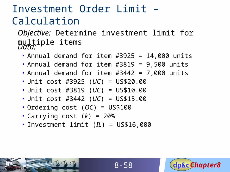
Investment Order Limit – Calculation
Objective: Determine investment limit for multiple items
Data: • Annual demand for item #3925 = 14,000 units• Annual demand for item #3819 = 9,500 units• Annual demand for item #3442 = 7,000 units• Unit cost #3925 (UC) = US$20.00• Unit cost #3819 (UC) = US$10.00• Unit cost #3442 (UC) = US$15.00• Ordering cost (OC) = US$100• Carrying cost (k) = 20%• Investment limit (IL) = US$16,000
Chapter8dp&c8-59
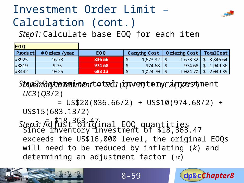
Investment Order Limit – Calculation (cont.)
Step1: Calculate base EOQ for each itemEOQProduct # Orders / year EOQ Carrying Cost Ordering Cost Total Cost
#3925 16.73 836.66 1,673.32$ 1,673.32$ 3,346.64$ #3819 9.75 974.68 974.68$ 974.68$ 1,949.36$ #3442 10.25 683.13 1,024.70$ 1,024.70$ 2,049.39$
Step2: Determine total inventory investmentInventory investment = UC1(Q1/2) + UC2(Q2/2) + UC3(Q3/2)
= US$20(836.66/2) + US$10(974.68/2) + US$15(683.13/2) = $18,363.47
Step3: Adjust original EOQ quantitiesSince inventory investment of $18,363.47 exceeds the US$16,000 level, the original EOQs will need to be reduced by inflating (k) and determining an adjustment factor (a)
Chapter8dp&c8-60
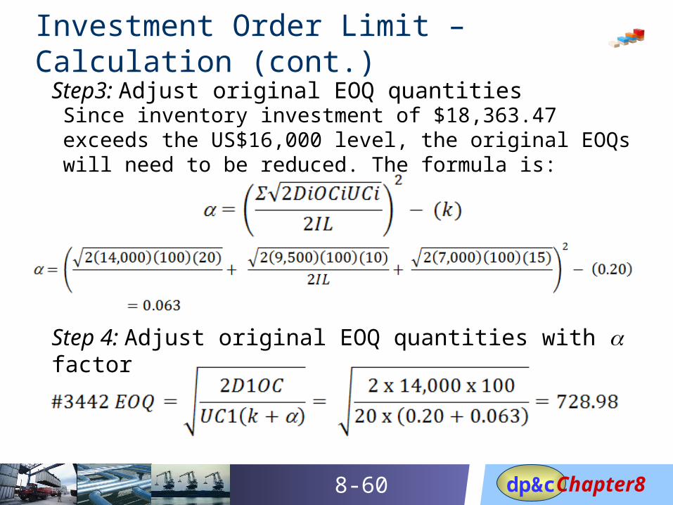
Investment Order Limit – Calculation (cont.)
Step3: Adjust original EOQ quantitiesSince inventory investment of $18,363.47 exceeds the US$16,000 level, the original EOQs will need to be reduced. The formula is:
Step 4: Adjust original EOQ quantities with a factor
Chapter8dp&c8-61
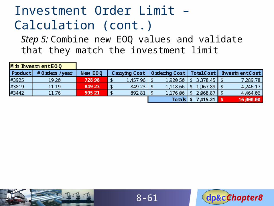
Investment Order Limit – Calculation (cont.)
Step 5: Combine new EOQ values and validate that they match the investment limit
Min Investment EOQProduct # Orders / year New EOQ Carrying Cost Ordering Cost Total Cost Investment Cost
#3925 19.20 728.98 1,457.96$ 1,920.50$ 3,378.45$ 7,289.78$ #3819 11.19 849.23 849.23$ 1,118.66$ 1,967.89$ 4,246.17$ #3442 11.76 595.21 892.81$ 1,176.06$ 2,068.87$ 4,464.06$
Totals 7,415.21$ 16,000.00$
Chapter8dp&c8-62
Inventory Management Basics
Chapter 8Statistical Inventory Management
Lean Inventory Management
Chapter8dp&c8-63
Defining Lean
A management and operations philosophy based on the planned minimization of all resources, the
continuous improvement of productivity, and a relentless search to convert product and process waste into customer winning value both within the
enterprise and outside in the supply chain.
APICS Dictionary, 13th edition
Chapter8dp&c8-64
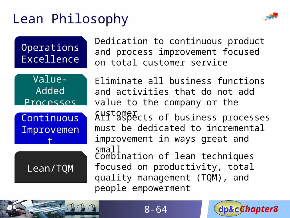
Lean Philosophy
Operations Excellence
Dedication to continuous product and process improvement focused on total customer service
Value-Added Processes
Eliminate all business functions and activities that do not add value to the company or the customer
Continuous Improvement
All aspects of business processes must be dedicated to incremental improvement in ways great and small
Lean/TQMCombination of lean techniques focused on productivity, total quality management (TQM), and people empowerment
Chapter8dp&c8-65
Lean Tactics to Reduce Inventory
•Focus on continuous inventory reduction
•Implement an inventory pull system
•Establish lean ordering and delivery with suppliers
•Deliver inventory directly to the point of use
•Map and streamline inventory flows
•Reduce batch sizes and production queues
•Reduce setup times
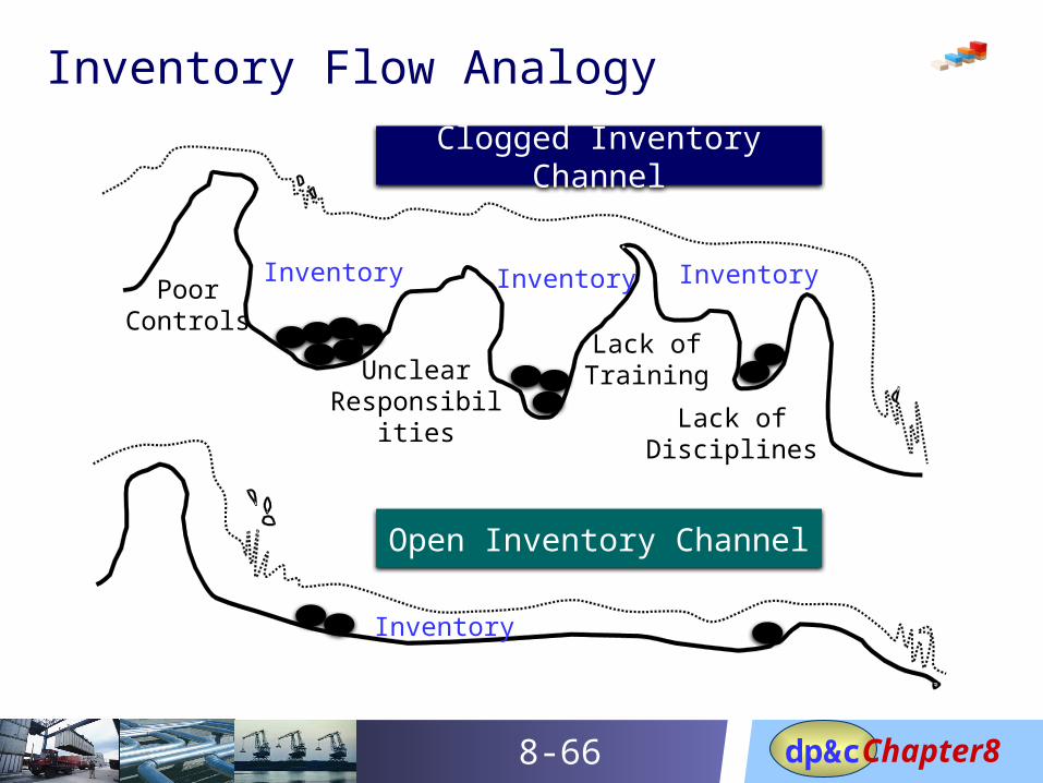
Chapter8dp&c8-66
Inventory Flow Analogy
PoorControls
UnclearResponsibilities
Lack ofTraining
Lack ofDisciplines
Clogged Inventory Channel
Open Inventory Channel
Inventory Inventory Inventory
Inventory
Chapter8dp&c8-67
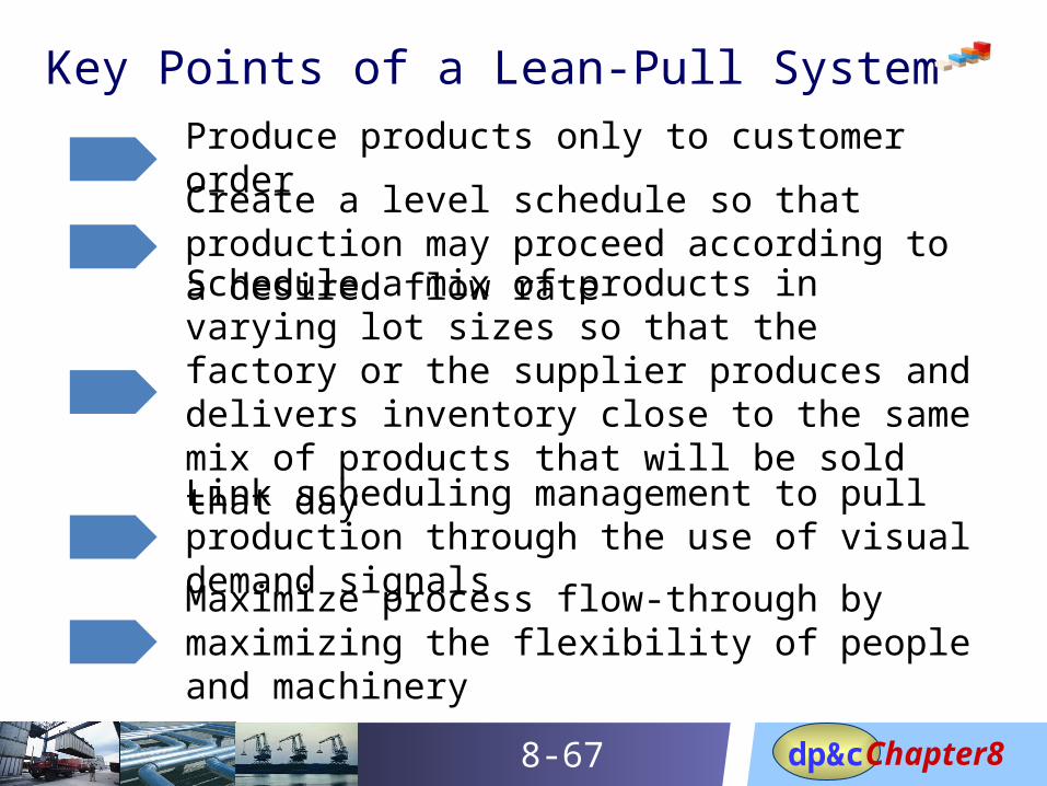
Key Points of a Lean-Pull System
Produce products only to customer order
Create a level schedule so that production may proceed according to a desired flow rate
Schedule a mix of products in varying lot sizes so that the factory or the supplier produces and delivers inventory close to the same mix of products that will be sold that day
Link scheduling management to pull production through the use of visual demand signals
Maximize process flow-through by maximizing the flexibility of people and machinery
Chapter8dp&c8-68
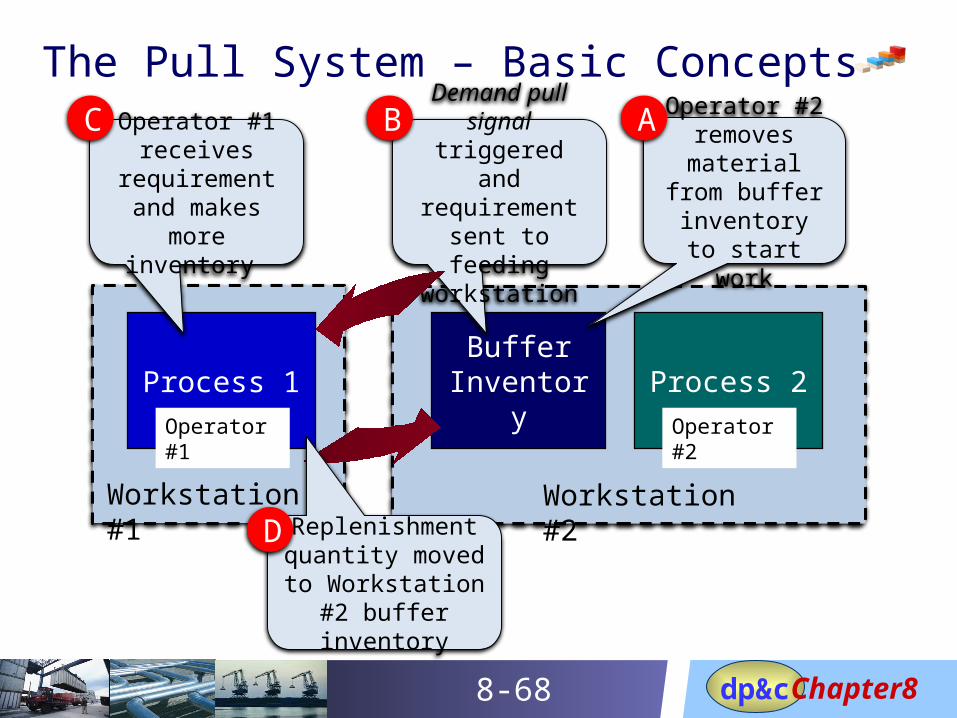
The Pull System – Basic Concepts
Process 2Buffer
Inventory
Workstation #2
Process 1
Operator #2 removes
material from buffer inventory
to start work
Demand pull signal triggered and requirement sent to feeding
workstation
Operator #1 receives
requirement and makes more
inventory
Replenishment quantity moved to
Workstation #2 buffer inventory
Workstation #1
ABC
D
Operator #1 Operator #2
Chapter8dp&c8-69
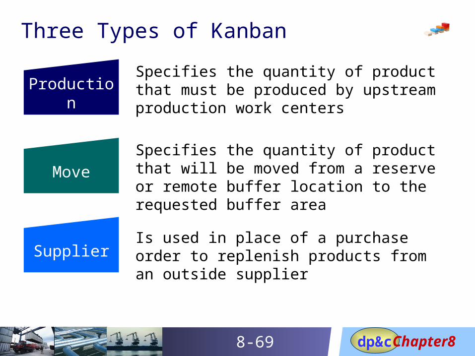
Three Types of Kanban
ProductionSpecifies the quantity of product that must be produced by upstream production work centers
MoveSpecifies the quantity of product that will be moved from a reserve or remote buffer location to the requested buffer area
SupplierIs used in place of a purchase order to replenish products from an outside supplier
Chapter8dp&c8-70
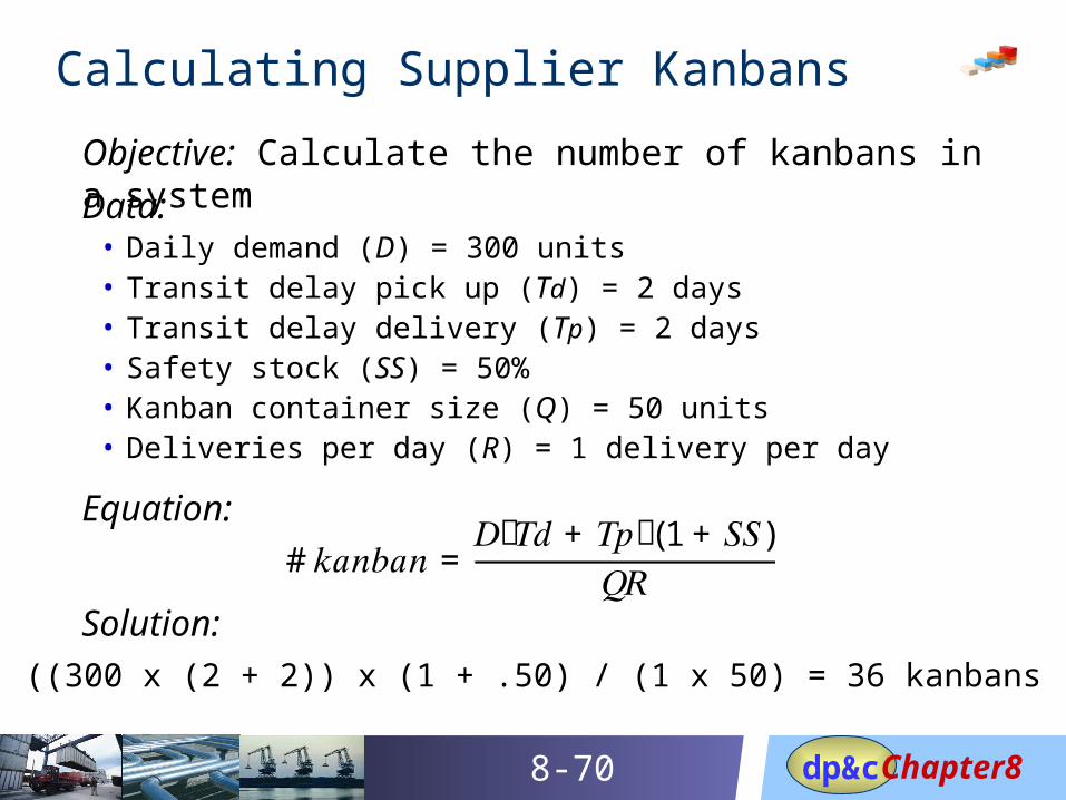
Calculating Supplier Kanbans
Objective: Calculate the number of kanbans in a system
Data: • Daily demand (D) = 300 units• Transit delay pick up (Td) = 2 days• Transit delay delivery (Tp) = 2 days• Safety stock (SS) = 50%• Kanban container size (Q) = 50 units• Deliveries per day (R) = 1 delivery per day
Equation: # 𝑘𝑎𝑛𝑏𝑎𝑛 = 𝐷ሺ𝑇𝑑+ 𝑇𝑝ሻ(1+ 𝑆𝑆)𝑄𝑅
Solution:
((300 x (2 + 2)) x (1 + .50) / (1 x 50) = 36 kanbans

Chapter8dp&c8-71
Chapter 8
End of Session
“Education in Pursuit of Supply Chain Leadership”
Chapter8dp&c
Recommended