57

CHAPTER 4. TAGGING METHODS AND ASSOCIATED DATA ANALYSIS

Robert J. Latour, Virginia Institute of Marine Science, College of William and Mary, PO Box 1346,

Gloucester Point, VA 23062 USA

4.1 INTRODUCTION

4.2 TAG TYPE AND PLACEMENT

4.2.1 Petersen disc tag

4.2.2 Internal anchor tag

4.2.3 Rototag

4.2.4 Dart tag

4.3 DATA COLLECTION AND ANALYSIS

4.3.1 Delineation of nursery areas, habitat utilization, stock identification

4.3.2 Length/weight relationship

4.3.3 Growth rates

4.3.4 Gear selectivity

4.3.5 Movement

4.3.6 Survival/mortality

4.3.7 Spatial and temporal distribution, relative abundance

4.3.8 Species composition, size composition, sex ratio

4.4 ASSUMPTIONS OF TAG-RECOVERY STUDIES AND AUXILIARY STUDIES

4.5 ARCHIVAL TAGS

4.6 SUMMARY

4.7 REFERENCES

58

59

4.1 INTRODUCTION

Tagging methods have a long history of use as tools to study animal populations. Although the first

attempts to mark an animal occurred sometime between 218 and 201 B.C. (a Roman officer tied a note

describing plans for military action to the leg of a swallow, and when the bird was released, it returned to

its nest which was in close proximity to the military outpost in need of the information), it is uncertain

when fish were first marked (McFarlane et al., 1990). An early report published in The Compleat Angler

in 1653 by Isaak Walton described how private individuals tied ribbons to the tails of juvenile Atlantic

salmon (Salmo salar) and ultimately determined that Atlantic salmon returned from the sea to their natal

river (Walton and Cotton, 1898; McFarlane et al., 1990). Since the late 1800s, numerous fish tagging

experiments have been conducted, with an initial emphasis on salmonids, followed soon after by successful

attempts at tagging flatfish and cod. Pelagic species, namely Pacific herring (Clupea harengus pallasi)

and bluefin tuna (Thunnus thynnus), were successfully tagged in the early 1900s, while elasmobranch

tagging studies did not commence until the 1930s. Since 1945, large-scale tagging programs have been

initiated all over the world in an effort to study the biology and ecology of fish populations.

Modern tagging studies can be separated into two general categories. Tag-recovery studies are

those in which individuals of the target population(s) are tagged, released, and subsequently killed upon

recapture, as in a commercial fishery; while capture-recapture studies are designed to systematically tag,

release, and recapture individuals on multiple sampling occasions. The former study-type often facilitates

the establishment of a cooperative tagging program in which fish are tagged by both scientists and volun-

teer fishermen. The primary advantage of a cooperative program is the sheer volume of fish that can be

tagged each year, since it is possible to combine the efforts of scientists and a large number of volunteer

recreational and commercial fishermen. The latter study-type typically leads to the creation of agency- or

institution-based tagging program in which only those scientists directly involved with the study tag fish.

When starting a tagging program, the choice of whether to design a tag-recovery study (that may

or may not be cooperative) or a capture-recapture study largely depends on the objectives of the tagging

program. For example, although tag-recovery studies tend to be much less labor intensive than capture-

recapture studies, the analysis of tag-recovery data does not easily yield estimates of population size,

which is often of interest to fisheries managers. Similarly, the quality of the data associated with a coop-

erative tag-recovery study can sometimes be suspect, since the level of tagging experience and overall

commitment to the tagging program in terms of the precision of the data being collected at the time of

tagging can vary significantly among fishermen. However, in some situations, it may not be possible to

develop a tagging program without the help of volunteer fishermen, since a single agency may not be able

to assume the cost associated with capturing and tagging hundreds or possibly thousands of fish each year.

The intent of this chapter is to serve as an overview of tagging studies and their use as tools for

increasing our biological understanding of elasmobranch populations and ultimately the information from

which we base management decisions. In a practical sense, however, it is virtually impossible in a single

60

chapter to adequately discuss all of the various aspects of tagging studies and the analysis of tagging data.

As such, this chapter will focus on issues related to tag-recovery programs and the analysis of tag-

recovery data, primarily because the cost effectiveness of these types of studies has rendered them a very

common approach for inferring life history characteristics of aquatic populations. The chapter begins with

a discussion of the various tag types that can be used to mark individuals, followed by a treatment of the

various types of analysis methods that can be used to derive information from tag-recovery data. Not

included in the chapter is a stand-alone section on the design of tag-recovery studies, largely because it is

difficult to accommodate all types of data collection and subsequent analyses using a single study design.

That said, however, it is extremely important to base the development of a tag-recovery program on a

clearly and rigorously defined study design. I have chosen to address the details associated with sampling

and data collection procedures periodically throughout the text, and in accordance with the type of data

and analysis being discussed. For more information on the design of capture-recapture studies and the

associated methods for data analysis, efforts should be made to consult the comprehensive monographs

developed by Burnham et al. (1987) and Pollock et al. (1990).

4.2 TAG TYPE AND PLACEMENT

No single tag type (and therefore tagging technique) is appropriate for all species of sharks, or in

some instances, all life stages within a particular species. As such, great consideration should be given to

the choice of tag type when developing a tagging program. Factors that can be used to assist with the

selection of a tag include but need not be limited to (Wydoski and Emery, 1983; McFarlane et al., 1990;

Kohler and Turner, 2001):

• The objectives of the tagging study or program.

• The effect of the tag on the life history characteristics of the species under study, namely, reproduction,

survival, and growth.

• The durability, longevity, and stability of the tag.

• The stress associated with the capture, handling, and tagging process.

• The size and number of individuals to be tagged.

• Ease (or lack thereof) of tag application.

• Cost of purchasing the tags and conducting the tagging experiment.

• The amount and type of cooperation required among agencies, states, or countries for the tagging

study to be successful.

For studies involving teleost species, the number of different tag types that have been used to mark

individuals is fairly extensive (McFarlane et al., 1990). Although a similar diversity among tag types can be

documented for studies involving shark populations, the Petersen disc, internal anchor tag, Rototag, and

dart tag tend to be the most widely used (Kohler and Turner, 2001).

61

4.2.1 Petersen disc tag

The Petersen disc tag, which was developed by Petersen (1896), is one of the first tags ever used

to study fish populations. Although the Petersen disc tag has undergone several modifications over the

years, in essence, the tag is comprised of two plastic discs that are placed on each side of the individual

and connected by either a wire or a pin running through either the dorsal fin or the musculature at the base

of the dorsal fin (Figure 4.01). The tag information is generally printed on the discs. Petersen disc tags

were used in many of the early shark tagging studies, which studied the growth and movement of a variety

of shark species in the Pacific (Holland, 1957; Kato and Carvallo, 1967; Bane, 1968).

There are two key drawbacks associated with the use of Petersen disc tags. Specifically, they are

prone to fouling by barnacles and algae and they can severely limit body and fin thickness by restricting

growth, especially when used for long-term tagging studies. This restriction of growth can lead to splitting

and deterioration of the dorsal fin, particularly with immature sharks since their cartilaginous dorsal rays

tend to be softer than those of mature sharks, and also because they will experience a more dramatic

growth rate over time when compared to mature individuals (Kohler and Turner, 2001).

4.2.2 Internal anchor tag

Rounsefell and Kask (1943) discuss the development of the internal anchor tag, which was

designed to overcome some of the problems associated with the use of Petersen disc tags, particularly the

restriction of growth. There are two types of internal anchor tags. The first tag, which is sometimes

referred to as a “body cavity tag”, is small and rectangular in shape, and is inserted completely into the

body cavity through a small incision in the lower half of the body wall (Figure 4.01). All pertinent informa-

Figure 4.01 Types of internal and external tags typically used to tag sharks. The appropriateanatomical location for attachment is indicated for each tag-type.

Reward 2003-12

Petersen disc

Internal anchor tag (body cavity)

Internal anchor tag (button)

Reward 2003-2

Jumbo Rototag

ORI tag

Dart tag Call 1-800-555-4444 for reward 2003-89

62

tion is printed on the tag, which is typically made of plastic. The second tag is sometimes referred to as a

“button” tag and is comprised of a vinyl streamer attached to an elongated plastic disc (Figure 4.02). The

disc serves as the anchor and again it is inserted into the body cavity through a small incision in the body

wall, with the streamer protruding external to the individual. The tag information is usually printed on both

the plastic disc and the streamer (Figure 4.01).

Each type of internal anchor tag has been used for a variety of shark tagging studies (Olsen, 1953;

Grant et al., 1979; Hurst et al.,

1999). An advantage of internal

anchor tags is that they can be

retained for many years, which is

desirable given the longevity of

many shark species. In terms of

tag recovery, however, body cavity

tags are only detectable once an

individual is gutted. This character-

istic renders it impossible to

conduct a capture-recapture study

using this tag type. Button tags are

more visible than body cavity tags,

despite the fact that the streamers

are susceptible to fouling and

abrasion. The application of some type of antibiotic salve or antiseptic solution to the tagging wound is

recommended when using either type of internal anchor tag.

4.2.3 Rototag

Davies and Joubert (1967) describe the early use of Rototags, which were originally manufac-

tured by Daltons of Henley-on-Thames, UK for livestock tagging but have been adapted for marine and

wildlife tagging studies. The Jumbo Rototag (Figure 4.03) and the ORI tag (which is a modified Jumbo

Rototag) are typically applied with an applicator through a hole in the leading edge of the first dorsal fin

created by a leather punch (Figure 4.01). Both tag types are made from a high-grade nylon, with the

Jumbo Rototag being semirectangular in shape and the ORI tag more circular in shape. Early experiments

with the Jumbo Rototag indicated that the tag was susceptible to vertical movement due to the hydrody-

namics of swimming (Davies and Joubert, 1967). The suspicion that this vertical movement caused

swelling and irritation prompted the design of the ORI tag.

As with the Petersen disc tag, the Jumbo Rototag and ORI tag are susceptible to fouling and can

negatively influence growth. Nevertheless, these tags have been used in numerous tagging studies of

shark species (Kato and Carvallo, 1967; Thorson and Lacy, 1982; Stevens, 1990; Kohler et al., 1998).

Figure 4.02 A “button” internal anchor tag. The tag is comprisedof a vinyl streamer attached to an elongated plastic disc. The discserves as the anchor and it is inserted into the body cavity througha small incision in the body wall, with the streamer protrudingexternal to the individual.

63

Until 1988, they were the primary

tag used in the common skate

(Dipturus batis) tagging program

conducted off the west coast of

Scotland by the Science Department

of Glasgow Museums, and are also

used by the Central Fisheries Board

of Ireland for their blue shark tagging

program.

4.2.4 Dart tag

The origin of the dart tag can

be traced back to early tagging

studies of marine pelagic fish, par-

ticularly tunas (McFarlane et al.,

1990). The dart tag was developed

primarily to facilitate the safe and effective tagging of individuals in the water, since many pelagic species

attain sizes that are too large to be handled onboard a vessel. Relative to the original design, the dart tag

was modified for use on sharks (Casey, 1985) and a variety of types of dart tags have been used by

numerous tagging programs over the years (Kohler and Turner, 2001). Fundamentally, a dart tag is

comprised of a streamer, which can be made of monofilament line, vinyl, or nylon line that is attached to

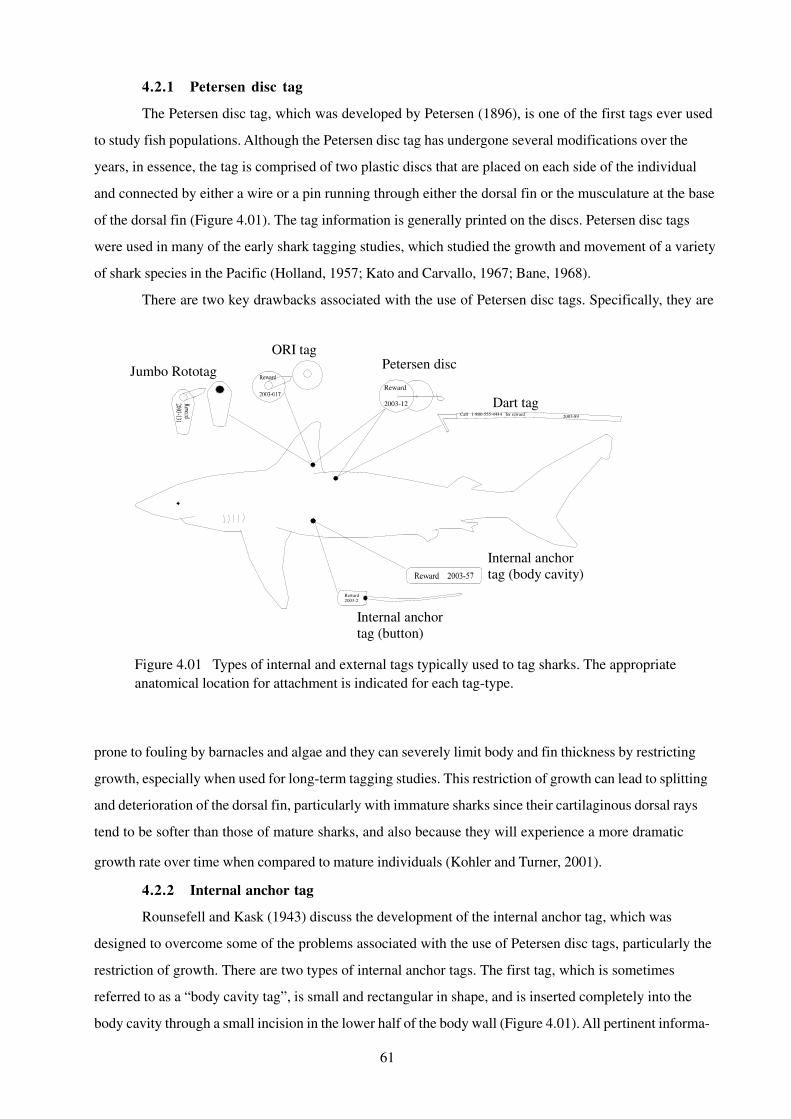
either a stainless steel, plastic, or nylon pointed head (Figure 4.01, Figure 4.04a). All pertinent tag informa-

tion is either printed on the streamer itself or on a legend that is enclosed by a capsule and attached to the

streamer. Application of a dart tag is usually accomplished using a stainless steel tagging needle, which is

used to drive the pointed head of the tag into the dorsal musculature of the individual (Figure 4.04b).

Efforts are generally made to apply the tag at an angle so that streamer lies alongside the individual while

it swims. For sharks, the optimal location for a dart tag is next to the base of the first dorsal fin.

The main advantage of using a dart tag is its ease of application. Relative to the Petersen disc tag,

Rototag, and internal anchor tag, very little time is needed to successfully mark an individual with a dart

tag. This characteristic combined with the fact that minimal training is necessary to become proficient at

applying a dart tag has rendered it the most commonly used tag type in shark tagging studies (Kohler and

Turner, 2001). Specific large-scale and longstanding tagging studies that utilize the dart tag include the

NMFS Cooperative Shark Tagging Program (Kohler et al., 1998; Kohler and Turner, 2001) and the

Australian Cooperative Game-Fish Tagging Program (Pepperell, 1990).

4.3 DATA COLLECTION AND ANALYSIS

Tag-recovery studies facilitate the collection of a variety of types of information on the species

under study. These data can be used to infer delineation of nursery areas, habitat utilization, stock identifi-

cation, length/weight relationships, growth rates, gear selectivity, patterns of movement, survival/mortality,

Figure 4.03 Jumbo rototag showing tag number and mailingaddress [from the NMFS Cooperative Shark Tagging Programwebsite (http://na.nefsc.noaa.gov/sharks/intro.html)].

64

spatial and temporal distribution, relative abundance, species and size composition and sex ratio (Kohler

and Turner, 2001). The following subsections contain a more detailed presentation of these data types and

their associated methods of analysis. With respect to deriving survival/mortality information from tag-

recovery data, my discussion is brief since a more complete treatment of the topic is provided in section

8.3.2 of Chapter 8.

While many of the aforementioned types of data are fairly simple and straightforward, it is still

important that they be collected under a rigorously defined sampling design. A commonly applied design is

a stratified random sampling design where the strata are defined according to variations in water depth,

salinity, water temperature or latitude/longitude. Although data collected haphazardly can provide anec-

dotal information about a particular species, subsequent analyses of those data will not yield accurate

inferences about the population as a whole. The choice of a sampling design and the subsequent sampling

gear often depend on a variety of factors, most notably the objective(s) of the study, the topography and

size of the study area, and the general life history characteristics of the species under study. Despite these

factors, a concept that is essential for deriving population level inferences is that the data collected are

representative of the target species in the study area. Hence, sampling should take place during all sea-

sons (unless the target species are not year-round residents) and over all spatial locations or habitat types

that the target species occupies within the study area. Clearly, temporal and spatial information may not be

available for species and areas that are not well studied, which implies that a very non-tailored and sys-

tematic sampling design must be adopted. Also, efforts should be made to sample with a gear-type that is

relatively non-selective; that is, one that will capture a wide variety of species and that will capture males

and females of all sizes with approximately equal probability. In practice, this need may render a longline

more appropriate than a gillnet.

Figure 4.04 (a) An “M” type dart tag display-ing tagging needle and legend [from the NMFSCooperative Shark Tagging Program website(http://na.nefsc.noaa.gov sharks/intro.html)];(b) application of a dart tag to an individualalong side a vessel [photo by J. A. Musick].

a. b.

65

4.3.1 Delineation of nursery areas, habitat utilization, stock identification

It is possible but often very difficult to use data reflecting the location of tag recoveries to effec-

tively delineate the nursery area of a species. Provided that an adequate number of young-of-the-year

(YOY) could be tagged and, of those, an adequate number of tag recoveries are tabulated, information on

the location of tag recoveries can be used to determine the habitat utilization and extent of the nursery

area for YOY individuals. In addition, if a representative sample of a species in a particular location is

tagged (i.e., individuals of varying sizes from both sexes in the area), it may be possible to determine the

habitat range of the whole population. Moreover, if several population level ranges have been delineated,

inferences about the degree to which various stocks mix and ultimately stock identification can be in-

ferred. However, the generally low tag-recovery rates observed with most elasmobranch species com-

bined with inaccurate reporting of recapture location from fishers can render it difficult to accurately

characterize habitat ranges.

An alternative approach to using the locations of tag recoveries to delineate the range of a popula-

tion is to infer about habitat utilization from the spatially explicit catch data obtained from sampling efforts

designed to capture individuals for tagging. Note that data resulting from supplemental sampling efforts

that are designed to “canvas” the suspected range or study area will likely be needed. This approach was

used by Grubbs (2001) to characterize the nursery ground of YOY sandbar sharks (Carcharhinus

plumbeus) in Chesapeake Bay. Although it was known that the Bay served as a nursery area for YOY

sandbar sharks, the exact geographical area within the Bay utilized by YOY sandbar sharks was not

known. Hence, Grubbs (2001) added stations to the sampling protocol of an existing longline survey in

such a manner as to systematically sample for the presence of YOY sharks from the Bay mouth north-

ward. The northernmost latitude of the nursery area was determined by noting the location where the

catches of YOY sandbar sharks became zero.

A second alternative approach that can be used to delineate habitat utilization and discern degrees

of site fidelity involves the use of acoustic telemetry (see section 8.3.3 of Chapter 8 for more information

on telemetry). To conduct a telemetry study, high-power, ultrasonic transmitters must be surgically or

externally implanted in a representative sample of the target species. Receivers are then used to monitor

transmitter output for the purpose of intermittently tracking the movements and space utilization of tagged

individuals. Prior to conducting the study, a tracking protocol that specifies the length of the tracking

session, the number of fish tracked each session, and frequency at which position information is obtained

should be developed. If previous telemetry studies have been conducted for the species under study, it is

recommended to adopt the same tracking protocol so that the data are comparable. Morrissey and Gruber

(1993) used acoustic telemetry to examine the spatial and temporal patterns of activity of juvenile lemon

sharks (Negaprion brevirostris) in the Bahamas. The study was the first to utilize nonarbitrary sampling

and successfully characterized patterns of movement and degree of site fixity in any elasmobranch

species. The study also examined the correlation between size of habitat range and body size.

66

4.3.2 Length/weight relationship

The observed length and weight measurements taken at the time of first capture can be used to

establish a number of predictive relationships. For example, it is often useful to develop conversions among

the various length measurements, which can usually be accomplished using simple linear regression:

21 LL βα += , (4.1)

where L1 and L

2 are the two length measurements (e.g., fork and total length (FL, TL), or FL and

precaudal length (PCL), etc.) for which a predictive relationship is desired, and α and β are the standard

simple linear regression parameters that are to be estimated. Prior to applying equation 4.1, it is recom-

mended to plot the length measurements against each other to ensure that a linear trend is present. Efforts

should also be made to develop length conversion relationships for males and females separately, as well

as for the sexes combined. As an example, see the FL/TL relationship derived by Natanson et al. (1999)

for tiger sharks (Galeocerdo cuvier) in the western North Atlantic.

In addition to predictive relationships among various types of length measurements, it is also

possible to use the size data collected at the time of first capture to establish a length/weight predictive

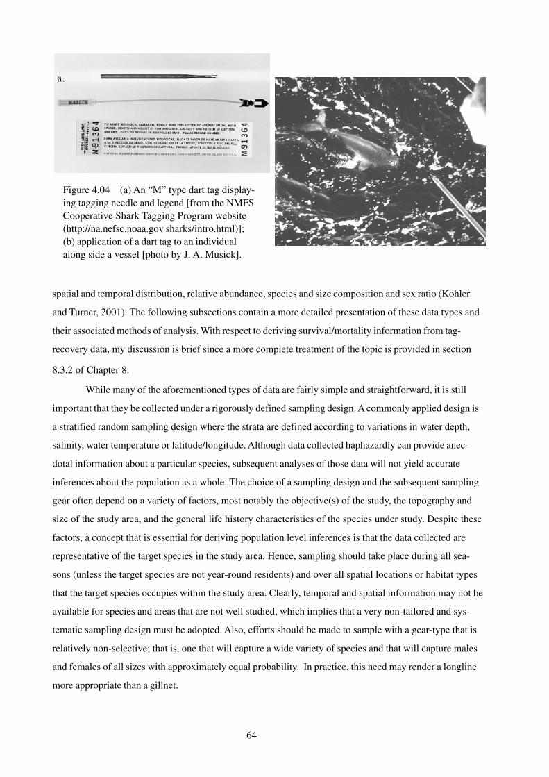
relationship. This type of relationship is typically derived using the following power function (Figure 4.05).

W = αLβ, (4.2)

where W and L represent weight and length, respectively, and α and β are regression parameters (not to

be confused with those of equation 4.1). Nonlinear regression techniques (Bates and Watts, 1988) can be

used to estimate α and β , and it is generally recommended to fit equation 4.2 to sex-specific as well as

combined length/weight data. Stevens (1990) applied equation 4.1 to length/weight data obtained at the

time of tagging for tope sharks (Galeorhinus galeus), blue sharks (Prionace glauca), and porbeagle

sharks (Lamna nasus) off the coast of England.

Despite the fact that equation 4.2 is frequently used to relate length and weight data, it should be

noted that it might not always be the most appropriate model. When attempting to derive a predictive

relationship between any variables, it is reasonable to fit several models to the data. Alternative models

for length/weight relationships might include a linear, quadratic, or change-point model, which is a piece-

wise function that is designed to fit two or more models each to separate portions of the data (Chappell,

1989). By fitting a suite of models to the data, it is then possible to use model selection techniques, notably

likelihood ratio tests and/or Akaike’s Information Criterion (AIC) and related measures (Burnham and

Anderson, 1998) to assess model performance and ultimately identify the model that best fits the data.

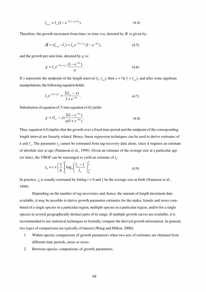
4.3.3 Growth rates

If fishers record the date and length when tagged fish are recaptured, then information on growth

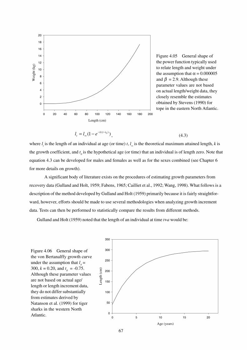
increments can be obtained and ultimately used to estimate the parameters of the von Bertalanaffy (1938)

growth function (VBGF). An obvious advantage to this approach is that a VBGF can be defined in the

absence of age data. The VBGF takes the form (Figure 4.06):

67

)1( )( 0ttkt ell −−

∞ −= , (4.3)

where lt is the length of an individual at age (or time) t, l∞ is the theoretical maximum attained length, k is

the growth coefficient, and t0 is the hypothetical age (or time) that an individual is of length zero. Note that

equation 4.3 can be developed for males and females as well as for the sexes combined (see Chapter 6

for more details on growth).

A significant body of literature exists on the procedures of estimating growth parameters from

recovery data (Gulland and Holt, 1959; Fabens, 1965; Cailliet et al., 1992; Wang, 1998). What follows is a

description of the method developed by Gulland and Holt (1959) primarily because it is fairly straightfor-

ward, however, efforts should be made to use several methodologies when analyzing growth increment

data. Tests can then be performed to statistically compare the results from different methods.

Gulland and Holt (1959) noted that the length of an individual at time t+a would be:

Length (cm)

0 20 40 60 80 100 120 140 160 180 200

Wei

ght (

kg)

0

2

4

6

8

10

12

14

16

18

20

Figure 4.05 General shape ofthe power function typically usedto relate length and weight underthe assumption that α = 0.000005and β = 2.9. Although theseparameter values are not basedon actual length/weight data, theyclosely resemble the estimatesobtained by Stevens (1990) fortope in the eastern North Atlantic.

Age (years)

0 5 10 15 20

Len

gth

(cm

)

0

50

100

150

200

250

300

350

Figure 4.06 General shape ofthe von Bertanalffy growth curveunder the assumption that l

4 =

300, k = 0.20, and t0 = -0.75.

Although these parameter valuesare not based on actual age/length or length increment data,they do not differ substantiallyfrom estimates derived byNatanson et al. (1999) for tigersharks in the western NorthAtlantic.

68

)1( )( 0 attkat ell +−−

∞+ −= . (4.4)

Therefore, the growth increment from time t to time t+a, denoted by δl, is given by:

)1()( )( 0 kattktat eellll −−−

∞+ −=−=δ , (4.5)

and the growth per unit time, denoted by g, is:

a

eelg

kattk )1()( 0

−−−

∞−= . (4.6)

If x represents the midpoint of the length interval (lt, l

t+a), then x = ½( l

t + l

t+a), and after some algebraic

manipulations, the following equation holds:

kattk

e

xlel −

∞−−∞ +

−=1

)(2)( 0 . (4.7)

Substitution of equation (4.7) into equation (4.6) yields:

)1(

)1(2)( ka

ka

ea

exlg −

−

∞ +−−= . (4.8)

Thus, equation 4.8 implies that the growth over a fixed time period and the midpoint of the corresponding

length interval are linearly related. Hence, linear regression techniques can be used to derive estimates of

k and l∞. The parameter t0 cannot be estimated from tag-recovery data alone, since it requires an estimate

of absolute size at age (Natanson et al., 1999). Given an estimate of the average size at a particular age

(or time), the VBGF can be rearranged to yield an estimate of t0:

⎥⎦

⎤⎢⎣

⎡⎟⎟⎠

⎞⎜⎜⎝

⎛ −⎟⎠⎞

⎜⎝⎛+=

∞

∞

l

ll

ktt t

elog1

0 . (4.9)

In practice, t0 is usually estimated by letting t = 0 and l

t be the average size at birth (Natanson et al.,

1999).

Depending on the number of tag-recoveries and, hence, the amount of length increment data

available, it may be possible to derive growth parameter estimates for the males, female and sexes com-

bined of a single species in a particular region, multiple species in a particular region, and/or for a single

species in several geographically distinct parts of its range. If multiple growth curves are available, it is

recommended to use statistical techniques to formally compare the derived growth information. In general,

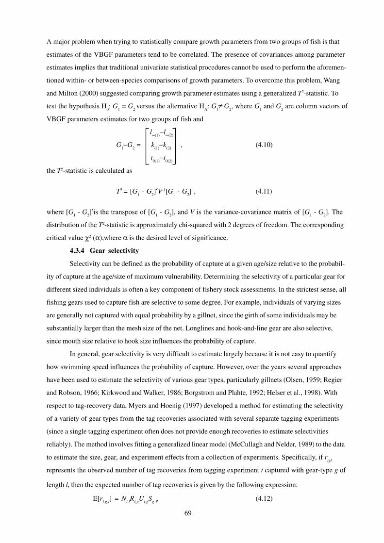
two types of comparisons are typically of interest (Wang and Milton, 2000):

1. Within-species comparisons of growth parameters when two sets of estimates are obtained from

different time periods, areas or sexes.

2. Between-species comparisons of growth parameters.

69

A major problem when trying to statistically compare growth parameters from two groups of fish is that

estimates of the VBGF parameters tend to be correlated. The presence of covariances among parameter

estimates implies that traditional univariate statistical procedures cannot be used to perform the aforemen-

tioned within- or between-species comparisons of growth parameters. To overcome this problem, Wang

and Milton (2000) suggested comparing growth parameter estimates using a generalized T2-statistic. To

test the hypothesis H0: G

1 = G

2 versus the alternative H

A: G

1 G

2, where G

1 and G

2 are column vectors of

VBGF parameters estimates for two groups of fish and

l∞(1)−l∞(2)

G1−G

2 = k

(1)−k

(2) , (4.10)

t0(1)

−t0(2)

the T2-statistic is calculated as

T2 = [G1 - G

2]′V-1[G

1 - G

2] , (4.11)

where [G1 - G

2]′is the transpose of [G

1 - G

2], and V is the variance-covariance matrix of [G

1 - G

2]. The

distribution of the T2-statistic is approximately chi-squared with 2 degrees of freedom. The corresponding

critical value χ2 (α),where α is the desired level of significance.

4.3.4 Gear selectivity

Selectivity can be defined as the probability of capture at a given age/size relative to the probabil-

ity of capture at the age/size of maximum vulnerability. Determining the selectivity of a particular gear for

different sized individuals is often a key component of fishery stock assessments. In the strictest sense, all

fishing gears used to capture fish are selective to some degree. For example, individuals of varying sizes

are generally not captured with equal probability by a gillnet, since the girth of some individuals may be

substantially larger than the mesh size of the net. Longlines and hook-and-line gear are also selective,

since mouth size relative to hook size influences the probability of capture.

In general, gear selectivity is very difficult to estimate largely because it is not easy to quantify

how swimming speed influences the probability of capture. However, over the years several approaches

have been used to estimate the selectivity of various gear types, particularly gillnets (Olsen, 1959; Regier

and Robson, 1966; Kirkwood and Walker, 1986; Borgstrom and Plahte, 1992; Helser et al., 1998). With

respect to tag-recovery data, Myers and Hoenig (1997) developed a method for estimating the selectivity

of a variety of gear types from the tag recoveries associated with several separate tagging experiments

(since a single tagging experiment often does not provide enough recoveries to estimate selectivities

reliably). The method involves fitting a generalized linear model (McCullagh and Nelder, 1989) to the data

to estimate the size, gear, and experiment effects from a collection of experiments. Specifically, if rigl

represents the observed number of tag recoveries from tagging experiment i captured with gear-type g of

length l, then the expected number of tag recoveries is given by the following expression:

E[ri,g,l

] = Ni,l

Ri,g

Ui,g

Sg l

, (4.12)

≠

70

where N is the number of individuals tagged, R is the product of the fraction of individuals that survive the

tagging process, the proportion of tags not shed, and the proportion of recovered tags that are reported

(which is assumed to be constant over length), U is the exploitation rate, and S is the selectivity (which is

assumed to be constant over the experiments included in the analysis). If the probability of capturing a

tagged individual is modeled as pi,g,l

= Ri,g

Ui,g

Sg l

, the generalized linear model takes the form:

log(πi,g,l

) = log(Ri,g

) + log(Ui,g

) + log(Sg,l

). (4.13)

Equation 4.13 possesses the three features of a generalized linear model: the function is linear, the

expected value of the dependent variable is related to the linear combination of the explanatory variables

via a link function (in this case the log link), and the error distribution is in the exponential family (in this

case a binomial error since the probability of observing rigl

tag recoveries is a binomial random variable).

Inherent to the method are the assumptions that tag-induced mortality, natural mortality, tag loss,

and tag-reporting rate are independent of fish length for each gear type and that growth and natural

mortality are small enough to be ignored during the analysis. To avoid violation of the latter assumption,

Myers and Hoenig (1997) recommend only considering tag-recoveries associated with individuals that

were at liberty for only a short period of time. Although this method has never been applied to elasmo-

branch tag-recovery data, Myers and Hoenig (1997) applied it to 137 tagging experiments of Atlantic cod

(Gadus morhua) and showed that the selectivity of otter trawls changed from the 1960s to the 1980s and

that the selectivity pattern assumed in several of the cod stock assessments was incorrect.

4.3.5 Movement

One of the principal objectives of most elasmobranch tag-recovery studies is to derive information

on movement. Over the years, there have been numerous studies documenting the patterns of movement

and space utilization for shark species worldwide. For example, Francis (1988) described the inshore-

offshore movements of rig (Mustelus lenticulatus) in New Zealand, Gruber et al. (1988) and Morrissey

and Gruber (1993) collectively described patterns of movement and home range for lemon sharks in the

Bahamas, and Casey and Kohler (1992) characterized the movement of shortfin mako sharks (Isurus

oxyrinchus) in the western north Atlantic. Many more examples of studies that derived information on the

movement of sharks from tag-recovery data can be found in the literature (see Kohler and Turner (2001)

for comprehensive list of these studies).

Efforts aimed at documenting patterns of activity and space utilization from tag-recovery data

typically begin by calculating the distance traveled and the time at liberty for each recaptured individual.

From those calculations, population-level estimates of movement can be determined by calculating the

mean and median distance traveled and the total range of distances (minimum and maximum) traveled. In

general, data associated with individuals that were recaptured within a short time of tagging are typically

71

excluded from distance calculations, largely because it is important to allow newly tagged individuals

enough time to become fully mixed into the overall tagged population (mixing ensures that tagged popula-

tion is representative of the total population). However, the decision to exclude these “immediate” recap-

tures does often depend on the objectives of the study. Although there is no “official” amount of time to

allow for mixing, Francis (1988) omitted all recaptures that were within 20 days of the time of tagging in

the movement analysis of rig.

As with the growth increment data, if there is a sufficient number of tag recoveries, it may be

possible to develop relationships between distance traveled and time at liberty for the males, female and

sexes combined of a single species in a particular region, multiple species in a particular region, and/or for

a single species in several geographically distinct parts of its range. If multiple characterizations of move-

ment are available, it is recommended to use statistical techniques to formally compare the derived move-

ment information. Two types of statistical analyses can be used to perform these comparisons:

1. A simple t-test, which tests for statistical differences between the mean distances traveled by two

groups (e.g., males and females of a particular species; sexes combined for two species; a

species in two regions of its geographic distribution, etc.).

2. Analysis of variance (ANOVA), which tests for statistical differences between the mean dis-

tances traveled by several groups (e.g., males and females of species in several locations of its

geographical distribution).

A two sample t-test can be used to test the hypotheses H0: d

1 = d

2 versus H

A: d

1 ≠ d

2, where d

1

and d2 represent the mean distance traveled for the two groups being compared, respectively. An equiva-

lent form of the hypotheses is H0: d

1 - d

2 = 0 versus H

A: d

1 - d

2 ≠ 0, and the t-value for testing these

hypotheses is:

t = _____________ , (4.14)

where n1 and n

2 represent the sample sizes of the two groups, respectively, and s

p is the pooled standard

deviation, which is calculated as a weighted average of the two sample variances S1

2 and S2

2:

(n1_1)s

12 + (n

2 _ 1)s

22

n1 + n

2 _2

The test statistic calculated from equation 4.14 can be compared to the critical value and H0 is rejected if

t< - tα/2,v or if t<tα/2

,v, where α is the significance level and v = n1+n

2 –2 is the degrees of freedom. The

two-sample t-test assumes that both samples are randomly chosen from normal populations with equal

variances (Zar, 1999). In practice, it is difficult to know if these assumptions will be met, however, several

studies have shown that the t-test is robust enough to endure considerable departures from its theoretical

assumptions, particularly when the sample sizes are equal or nearly equal (Zar, 1999).

d1 _ d

2

1 + 1

n1 n

2

Sp

Sp

= ,(4.15)

72

As stated previously, the above t-test is appropriate for situations when two means are being

compared, however, to test the hypotheses H0: d

1 = d

2 = … = d

k, where k is the number of groups being

compared, versus HA: not H

0, the procedure of ANOVA must be used. ANOVA is a large area of statisti-

cal methods and is not described in detail in this chapter. For more information on ANOVA, it is recom-

mended to consult a statistical methods textbook (e.g., Zar (1999)). For an example of ANOVA being

used to compare the mean distances traveled by several groups of a shark species, see Francis (1988).

4.3.6 Survival/mortality

Brownie et al. (1985) developed a series of models for multiyear tag recovery studies that can be

used to estimate age- and year-specific finite rates of survival (S) and tag recovery (f). More recently,

Pollock et al. (1991) and Hoenig et al. (1998) showed it is possible to convert tag-recovery rates to finite

exploitation (u), when information on the short-term tag retention, tag-induced mortality, and tag-reporting

rate is available. Estimates of year-specific total instantaneous mortality (Z) can be obtained from year-

specific finite rates of survival, and if information on the instantaneous rate of natural mortality (M) is

known, the year-specific estimates of Z can be used to recover year-specific estimates of instantaneous

fishing mortality (F) rates. Also, if the timing of the fishery is known, year-specific estimates of finite

exploitation can also be used to derive year-specific estimates of F (in the case of a continuous Type II

fishery, information on M will again be needed). A detailed discussion of these analyses is presented in

section 8.3.2 of Chapter 8.

4.3.7 Spatial and temporal distribution, relative abundance

Data reflecting the time and location of capture for tagging over the course of a year can be used

to develop a rudimentary understanding of seasonal habitat utilization, and thus, the spatial and temporal

distribution of the target species. In addition, the catch data derived from sampling efforts serves as a

spatial and temporal index of relative abundance for each species. One approach that can be used to

better understand the observed patterns of relative abundance involves correlating the spatially explicit

relative abundances with data that delineates habitat type (if not already available, this type of information

may need to be collected at the time of first capture). Although stand-alone correlations between catch

and habitat type are informative, it is often difficult to fully understand the observed patterns of relative

abundance without additional auxiliary data. Information on abiotic factors such as depth, water tempera-

ture, salinity and dissolved oxygen can also be used to help explain the observed patterns of distribution

and ultimately form a more complete understanding of the ecological preferences of the target species.

4.3.8 Species composition, size composition, sex ratio

Information on the species composition in a specific location or region and the sex ratio of a

particular species are two basic but important types of data that can be collected by simply processing the

catch of the gear used to collect individuals for tagging. In addition, when individuals are tagged onboard a

vessel, information on size composition can easily be obtained by taking sex-specific measurements of

73

length, which includes TL, FL, and PCL, and weight. Under circumstances when individuals are too large

to be handled and tagging takes place in the water, it may only be possible to take length measurements. In

areas where elasmobranchs are not well studied and information is lacking, collecting these types of data

can be viewed as the first step toward developing an understanding of the life history characteristics of the

species inhabiting a particular region.

4.4 ASSUMPTIONS OF TAG-RECOVERY STUDIES AND AUXILIARY STUDIES

When attempting to use tag-recovery data to infer about growth rates, gear selectivity, patterns of

movement, and survival/mortality, it is generally necessary to make the following assumptions:

1. The tagged sample is representative of the target population.

2. There is no tag loss or, if tag loss occurs, a constant fraction of tags is lost from each cohort and

all tag loss occurs immediately after tagging. Also, the probability of immediate tag loss is not sex-

or size-dependent.

3. The time and location of tagging and tag recovery are correctly recorded.

4. The lengths and weights of individuals are measured without bias at the time of tagging.

5. The lengths of individuals are measured without bias at the time of tag recovery.

6. Survival rates are not affected by tagging process or, if they are, the effect is restricted to a

constant fraction dying immediately after tagging. Also, the probability of immediate tag-induced

mortality is not sex- or size-dependent.

7. The fate of each tagged individual is independent of the other tagged individuals.

8. Tagging does not affect growth.

9. There are no significant size-selection processes for individuals within similar age ranges.

10. All tagged individuals within a cohort experience the same annual survival and tag-recovery rates.

11. The decision made by a fisher on whether or not to return a tag does not depend on when or

where the individual was tagged.

Although tag-recovery studies can be plagued by a variety of factors, it is possible to conduct auxiliary

studies to assess the possibility of violating a few of the aforementioned assumptions. Specifically, to

determine the rates of immediate tag loss and tag-induced mortality (assumptions 2 and 6), newly tagged

individuals can be held in cages or holding pens for a short period of time (Gruber et al., 2001;

Latour et al., 2001). Rates of chronic or long-term tag loss (assumption 2) are best assessed by double

tagging individuals (Latour et al., 2001). Although estimates of the tag-reporting rates associated with

commercial and recreational fishers are not needed for the types of analyses described herein, knowledge

of these tag-reporting rates can be extremely useful, particularly when trying to derive survival/mortality

information. Rates of tag reporting are best estimated by conducting a high reward study (Henny and

Burnham, 1976; Pollock et al., 2001). Additional remedies to some more of the problems of tag-recovery

studies as they pertain to survival/mortality estimation are discussed in section 8.3.2 of Chapter 8.

74

4.5 ARCHIVAL TAGS

Archival, or data storage tags are designed to intermittently record data on (among others) the

depth of an individual, ambient temperature, and light intensity. The data from these tags is downloaded

when the tagged fish is recaptured and the tag is recovered. These types of tags were first used on

southern bluefin tuna (Thunnus maccoyii) in Australia in the early 1990s, and have recently been used to

study elasmobranchs. Specifically, the Centre for Environment, Fisheries and Aquaculture Science

(CEFAS) Lowestoft Laboratory, which is located in the United Kingdom, has used archival tags to study

the movements of thornback rays (Raja clavata) in both the Irish Sea and Thames Estuary (Arnold and

Dewar, 2001). Similarly, Australia’s Commonwealth Scientific and Industrial Research Organisation

(CSIRO) has used archival tags to study the position of school sharks on the continential shelf off South

Australia (West and Stevens, 2001). One problem associated with an archival tagging study is the ex-

pense, since for many species, tag-recovery rates are too low to justify the cost of the tags. However, the

data from archival tags do have the potential to solve some important ecological questions (Arnold and

Dewar, 2001).

Pop-up archival satellite tags were developed in part to alleviate some of

the problems associated with low tag-recovery rates. In summary, these tags

combine data storage tags with satellite transmitters and are designed to detach

themselves from fish at a predetermined time (Figure 4.07). Ultimately they float to

the sea surface and communicate their location via a satellite link. The first pop-up

satellite tags were deployed in 1997 to further assist with ongoing efforts directed

at studying long-term movements of Atlantic bluefin tuna (Block et al., 1998).

Some of these tags were programmed to record temperature information on hourly

time scales, while others were programmed to take measurements on daily time

scales. Deployment time of these tags ranged from 3 to 90 days. Lutcavage et al.

(1999) also used pop-up satellite tags to study bluefin tuna in the North Atlantic.

Tags have also been successfully placed on other large pelagic species, including

yellowfin tuna, albacore, blue and striped marlin, and white, basking, thresher and

salmon sharks (Arnold and Dewar, 2001; Boustany et al., 2002).

There is a growing perception among researchers that some of the meth-

ods used to attach pop-up archival satellite tags to marine fishes are unreliable.

This perception originated from documented case studies were tags detached from

individuals prior to the predetermined time, thereby compromising the success of

the tagging study. However, the exact cause of the early release of these tags is

not known. Pop-up satellite tags are typically attached to pelagic teleosts via a dart

that is inserted into the dorsal musculature of the individual. For sharks, tags can be

attached using a dart or by attaching the tag to a rototag-like apparatus through a

Figure 4.07 WildlifeComputers Pop-upArchival Transmit-ting (PAT) tag.

75

hole in the first dorsal fin. To improve the retention and overall performance of pop-up satellite tags, a

variety of darts have been developed, ranging in terms of both shape and material used for construction.

At present, however, a universally accepted attachment method has not been identified, so for each

tagging study, great care should be directed at evaluating the potential effectiveness of each attachment

method as it pertains to the species under study.

4.6 SUMMARY

This chapter is designed to assist researchers with the development and implementation of a tag-

recovery program for elasmobranch species. As previously described, it is possible to initiate either an

angler-based cooperative program or an agency-based program, and in most cases, the objective(s) of the

study and available funding typically dictate the appropriate choice. Also, there are advantages and

disadvantages associated with each type of program that should be given consideration during the design

phase. Described in this chapter are several data analysis methods that can be used to infer various

aspects of the biology and life history of elasmobranch species. A wide variety of methodologies are

described in part to demonstrate the utility and usefulness of a tag-recovery program. Some inferences

can be drawn in the absence of data reflecting tag recoveries (e.g., habitat utilization, species and size

composition, sex ratio, etc. derived from catch data), while others require analysis of data from both first

capture and tag recovery (e.g., movement, growth, survival/mortality, etc.). Of particular importance to the

validity of any type of data analysis and to the overall success of a tag-recovery program is an assessment

of the potential for assumption violation. As a result, efforts should be directed at conducting auxiliary

studies to determine if the defined sampling, handling, and tagging protocol minimizes the potential for

assumption violation.

4.7 REFERENCES

ARNOLD, G., AND H. DEWAR. 2001. Electronic tags in marine fisheries research: a 30-year perspective, p. 7-

64. In: Electronic Tagging and Tracking in Marine Fisheries. J. R. Sibert and J. L. Nielsen (eds.).

Kluwer Academic Publishers, The Netherlands.

BANE, G. W. 1968. The great blue shark. California Currents 1:3-4.

BATES, D. M., AND D. G. WATTS. 1988. Nonlinear Regression Analysis and its Applications. John Wiley and

Sons, New York.

BLOCK, B. A., H. DEWAR, C. FARWELL, AND E. D. PRINCE. 1998. A new satellite technology for tracking

movements of Atlantic bluefin tuna. Proc. Natl. Acad. Sci. USA 95:9384-9389.

BORGSTROM, R., AND E. PLAHTE. 1992. Gill net selectivity and a model for capture probabilities of a stunted

brown trout (Salmo trutta) population. Can. J. Fish. Aquat. Sci. 49:1546-1554.

BOUSTANY, A. M., S. F. DAVIS, P. PYLE, S. D. ANDERSON, B. J. LEBOEUF, AND B. A. BLOCK. 2002. Satellite

tagging: expanded niche for white sharks. Nature 412:35-36.

76

BROWNIE C., D.R ANDERSON, K.P. BURHNAM, AND D.R. ROBSON. 1985. Statistical inference from band

recovery data: a handbook. U.S. Fish and Wildlife Service Resource Publication.

BURNHAM, K. P., AND D. R. ANDERSON. 1998. Model Selection and Inference: A Practical Information

Theoretical Approach. Springer-Verlag, New York.

__________, D. R. ANDERSON, G. C. WHITE, C. BROWNIE, AND K. H. POLLOCK. 1987. Design and analysis

methods for fish survival experiments based on release-recapture. American Fisheries Society,

Monograph 5, Bethesda, Maryland.

CAILLIET, G. M., H. F. MOLLET, G. C. PITTENGER, D. BEDFORD, AND L. J. NATANSON. 1992. Growth and

demography of the Pacific angel shark (Squatina californica), based upon tag returns off

California. Aust. J. Mar. Freshwat. Res. 43:1313-1330.

CASEY, J. G. 1985. Transatlantic migrations of the blue shark: a case history of cooperative shark tagging,

p. 253-268. In: World angling resources and challenges. R. H. Stroud (ed.). Proceedings of the

first world angling conference, Cap d’Agde, France, September 12-18, 1984, International Game

Fish Association, Ft. Lauderdale.

__________, AND N. E. KOHLER. 1992. Tagging studies on the shortfin mako shark (Isurus oxyrinchus)

in the Western North Atlantic. Aust. J. Mar. Freshwat. Res. 43:45-60.

CHAPPELL R. 1989. Fitting bent lines to data, with applications to allometry. J. Theoret. Biol. 138:235-256.

DAVIES, D. H., AND L. S. JOUBERT. 1967. Tag evaluation and shark tagging in South African waters, 1964-

65, p. 111-140. In: Sharks, skates, and rays. P. W. Gilbert, R. F. Mathewson, and D. P. Rall (eds.).

Johns Hopkins Press, Baltimore.

FABENS, A. J. 1965. Properties and fitting of the von Bertalanffy growth curve. Growth 29:265-289.

FRANCIS, M. P. 1988. Movement patterns of rig (Mustelus lenticulatus) tagged in southern New Zealand.

N.Z. J. Mar. Freshwat. Res. 22:259-272.

GRANT, C. J., R. L. SANDLAND, AND A. M. OLSEN. 1979. Estimation of growth, mortality, and yield per recruit

of the Australian school shark, Galeorhinus australis (Macleay), from tag recoveries. Aust. J.

Mar. Freshwat. Res. 30:625-637.

GRUBBS, R. D. 2001. Nursery delineation, habitat utilization, movements, and migration of juvenile

Carcharhinus plumbeus in Chesapeake Bay, Virginia, USA. Ph.D dissertation, Virginia Institute

of Marine Science, College of William and Mary, Gloucester Point, VA.

GRUBER, S. H., D. R. NELSON, AND J. F. MORRISSEY. 1988. Patterns of activity and space utilization of lemon

sharks, Negaprion brevirostris, in a shallow Bahamian lagoon. Bull. Mar. Sci. 43:61-76.

GRUBER, S. H., J. R. C. DE MARIGNAC, AND J. M. HOENIG. 2001. Survival of juvenile lemon sharks at Bimini,

Bahamas estimated by mark-depletion experiments. Trans. Am. Fish. Soc. 130:376-384.

GULLAND, J. A., AND S. J. HOLT. 1959. Estimation of growth parameters for data at unequal time intervals.

J. Cons. Int. Exp. Mer. 25:47-49.

77

HELSER, T. E., J. P. GEAGHAN, AND R. E. CONDREY. 1998. Estimating gillnet selectivity using nonlinear

response surface regression. Can. J. Fish. Aquat. Sci. 55:1328-1337.

HENNY, C. J., AND K. P. BURNHAM. 1976. A reward band study of mallards to estimate band reporting rates.

J. Wild. Manage. 40:1-14.

HOENIG, J. M., N. J. BARROWMAN, W. S. HEARN, AND K. H. POLLOCK. 1998. Multiyear tagging studies

incorporating fishing effort data. Can. J. Fish. Aquat. Sci. 55:1466-1476.

HOLLAND, G. A. 1957. Migration and growth of the dogfish shark, Squalus acanthias (Linnaeus), of the

eastern North Pacific. Washington Department of Fisheries, Fisheries Research Paper 2:43-59.

HURST, R. J., N. W. BAGLEY, G. E. MCGREGOR, AND M.P. FRANCIS. 1999. Movements of the New Zealand

school shark, Galeorhinus australis, from tag returns. N.Z. J. Mar. Freshwat. Res. 33:29-48.

KATO, S., AND A. H. CARVALLO. 1967. Shark tagging in the eastern Pacific Ocean, 1962-65, p. 93-109. In:

Sharks, skates, and rays. P. W. Gilbert, R. F. Mathewson, and D. P. Rall (eds.). Johns Hopkins

Press, Baltimore.

KIRKWOOD, G. P., AND T. I. WALKER. 1986. Gill net mesh selectivities for gummy shark, Mustelus

antarcticus Guenther, taken in south-eastern Australian waters. Aust. J. Mar. Freshwat. Res.

37:689-697.

KOHLER, N. E., AND P. A. TURNER. 2001. Shark tagging: a review of conventional methods and studies.

Environ. Biol. Fish. 60:191-223.

___________, J. G. CASEY, AND P. A. TURNER. 1998. NMFS cooperative shark tagging program, 1962-

1993: an atlas of shark tag and recapture data. Mar. Fish. Rev. 60:1-87.

LATOUR, R. J., K. H. POLLOCK, C. A. WENNER, AND J. M. HOENIG. 2001. Estimates of fishing and natural

mortality for red drum (Sciaenops ocellatus) in South Carolina waters. N. Am. J. Fish. Manage.

21:733-744.

LUTCAVAGE, M. E., R. W. BRILL, G. B. SKOMAL, B.C. CHASE, AND P. W. HOWEY. 1999. Results of pop-up

satellite tagging of spawning size class fish in the Gulf of Maine: do North Atlantic bluefin tuna

spawn in the mid-Atlantic? Can. J. Fish. Aquat. Sci. 56:173-177.

MCCULLAGH, P. AND J. A. NELDER. 1989. Generalized Linear Models. Chapman and Hall, 2nd edition.

MCFARLANE, G. A, R. S. WYDOSKI, AND E. D. PRINCE. 1990. Historical review of the development of exter-

nal tags and marks. Am. Fish. Soc. Symp. 7:9-29.

MORRISSEY, J. F., AND S. H. GRUBER. 1993. Home range of juvenile lemon sharks, Negaprion brevirostris.

Copeia 1993:425-434.

MYERS, R. A., AND J. M. HOENIG. 1997. Direct estimates of gear selectivity from multiple tagging experi-

ments. Can. J. Fish. Aquat. Sci. 54:1-9.

NATANSON, L. J., J. G. CASEY, N. E. KOHLER, AND T. COLKET IV. 1999. Growth of the tiger shark,

Galeocerdo cuvier, in the western North Atlantic based on tag returns and length frequencies;

and a note on the effect of tagging. Fish. Bull. 97:944-953.

78

OLSEN, A. M. 1953. The biology, migration, and growth rate of the school shark, Galeorhinus australis

(Macleay) (Carcharhanidae) in south-eastern Australian waters. Aust. J. Mar. Freshwat. Res.

5:353-410.

OLSEN, S. 1959. Mesh selection in herring gill nets. J. Fish. Res. Board Can. 16:339-349.

PEPPERELL, J. G. 1990. Australian cooperative game-fish tagging program, 1973-1987: status and evaluation

of tags. Am. Fish. Soc. Symp. 7:765-774.

PETERSEN, C. G. J. 1896. The yearly immigration of young plaice into the Limfjord from the German Sea.

Report of the Danish Biological Station to the Board of Agriculture (Copenhagen) 6:5-30.

POLLOCK, K. H., J. D. NICHOLS, C. BROWNIE, AND J. E. HINES. 1990. Statistical inference for capture-

recapture experiments. Wildl. Monogr. 107.

__________, HOENIG, J.M., AND JONES, C.M. 1991. Estimation of fishing and natural mortality when a

tagging study is combined with a creel survey or port sampling. Am. Fish. Soc. Symp. 12:423-434.

__________, J. M. HOENIG, W. S. HEARN, AND B. CALINGAERT. 2001. Tag reporting rate estimation: 1. An

evaluation of the high-reward tagging method. N. Am. J. Fish. Manage. 21:521–532.

REGIER, H. A., AND D. S. ROBSON. 1966. Selectivity of gillnets, especially to lake whitefish. J. Fish. Res.

Board Can. 23:423-454.

ROUNSEFELL, G. A., AND J. L. KASK. 1943. How to mark fish. Trans. Am. Fish. Soc. 73:320-363.

STEVENS, J. D. 1990. Further results from a tagging study of pelagic sharks in the north-east Atlantic. J.

Mar. Biol. Assoc. UK 70:707-720.

THORSON, T. B., AND E. J. LACY, JR. 1982. Age, growth rate and longevity of Carcharhinus leucas esti-

mated from tagging and vertebral rings. Copeia 1982:110-116.

VON BERTALANFFY, L. 1938. A quantitative theory of organic growth (Inquiries on growth laws. II). Human

Biology 10:141-147.

WALTON, I., AND C. COTTON. 1898. The compleat angler, of the contemplative man’s recreation. Little,

Brown, Boston.

WANG, Y. –G. 1998. An improved Fabens method for estimation of growth parameters in the von

Bertalanffy model with individual asymptotes. Can. J. Fish. Aquat. Sci. 55:397-400.

_________, AND D. A. MILTON. 2000. On comparison of growth curves: How do we test whether growth

rates differ? Fish. Bull. 98:874-880.

WEST, G. J., AND J. D. STEVENS 2001. Archival tagging of school shark, Galeorhinus galeus, in Australia:

initial results. Environ. Biol. Fish. 60:283-298.

WYDOSKI, R. S., AND L. EMERY. 1983. Tagging and marking, p. 215-237. In: Fisheries techniques. L. Neilsen

and D. Johnson (eds.). American Fisheries Society, Bethesda, Maryland.

ZAR, J. H. 1999. Biostatistical analysis, 4th edition. Prentice Hall, New Jersey.