1
7 November 2013
Rev 8
Chapter 4 DISSEMINATION OF THE ACCOUNTS AND STATIS TICS TO DIFFERENT TARGET AUDIENCES
This chapter discusses how the information compiled in the accounts is organized and presented to the different audiences. It shows how different types of indicators can be calculated from the accounts combining monetary and physical information. The chapter also presents the sequence of accounts as a means of calculating different balances useful to derive indicators, as well as for presenting the information. I. Information and indicators for different audiences • The information pyramid • Indicators for each of the policy quadrants • Core water tables II. Sequence of accounts to derive monetary balances and indicators • The sequence of accounts for water utilities • Interpretation of the accounts for water utilities • Scenarios of “tariffs” and changes in net worth • Types of indicators derived from the sequence of accounts III. Sequence of accounts to derive water flow balances and indicators • Sequence of water flows and tables • Types of indicators derived from the sequence of water flows • Minimum set of data to be collected about the water cycle • Emissions • Additional indicators derived from emission accounts • Minimum set of data to be collected about emissions

2
.I. Information and indicators for different audien ces The wide variety of data compiled through the process of integration of water accounts and statistics described in the previous chapters provides the platform for producing information aimed at a wide variety of users. Users of the information may include policy makers, the general public, managers, analysts, and researchers, among others. Understanding the needs of the information users or audiences is one of the most important considerations for disseminating information and indicators1. Different audiences will require the information with different levels of detail. Policy makers and the wider public generally require indicators and other forms of summary or aggregated information, while researchers may require a much higher level of detail, i.e. microdata. The following figure shows the information pyramid starting at the bottom with high level of detail information at the bottom and indicators, or highly aggregated information at the top. The SEEA and the SNA, as well as other statistical methodologies, provide the mechanisms for compiling the information to be able to derive indicators.
Figure 4.1.1 Information pyramid
Source: based in UNSD-IRWS
1 UNSD. International Recommendations for Water Statistics. 2012
Raw Data
Compilation
Indica-tors
Raw Data
Compilation
Indica-tors
Less detail
More detail

3
Compiling the information in order to produce different reports requires the use of a wide variety of statistical methodologies. The figure below shows some of the methodologies that are linked to the different components of the SEEA.
Figure 4.1.2 Set of statistical methodologies for compiling information The dissemination of information should be performed according to a set of principles. Chapter VIII of the IRWS provides several recommendations for the dissemination of information, including dissemination principles, as well as other relevant aspects to consider. Countries also provide information to a range of international organizations. There are several international initiatives collecting data from countries or agencies within countries, such as, FAO Aquastat, the OECD-Eurostat questionnaire, and the UNSD-UNEP water questionnaire. The information compiled according to the statistical methodologies presented in these Guidelines can be used to respond to all these international initiatives. To guide the data collection and compilation processes, as well as the dissemination process, information can be organized according to the four quadrants described in chapter 1 of these Guidelines. Each country can decide the level of detail for the data collection and compilation process for each of the groups. Depending on the level of detail and type of information to be collected, countries may decide to implement different sections of the SEEA, usually starting with those in the Central Framework (CF), and then moving to the SEEA Ecosystem Experimental Accounts.
Data
Data Quality Assessment Frameworks
Metadata and documentation (e.g. SDMX)
ISIC, CPC, Asset Classification, Class. of Environmental Activities, Class. of Physical Flows etc
DataData
Data Quality Assessment FrameworksData Quality Assessment Frameworks
Metadata and documentation (e.g. SDMX)Metadata and documentation (e.g. SDMX)
ISIC, CPC, Asset Classification, Class. of Environmental Activities, Class. of Physical Flows etcISIC, CPC, Asset Classification, Class. of Environmental Activities, Class. of Physical Flows etc
Input frameworksInput frameworks
Cross functional frameworks
Cross functional frameworks
SEEA
e.g. IRWS
Other water statistics
Compilation Material
SEEA-Water
e.g. IRWS
Other water statistics
e.g. IRWS
Other water statistics
Compilation MaterialCompilation Material
SEEA-WaterSEEA-Water
Energy balances
e.g. IRES
Compilation Material
SEEA-Energy
Energy balances
e.g. IRES
Energy balances
e.g. IRES
Compilation MaterialCompilation Material
SEEA-EnergySEEA-EnergyOutput frameworks
Systems frameworks
Intermediate frameworks
Output frameworks
Systems frameworks
Intermediate frameworks

4
The following information and indicators can be derived from the accounts for each group, as described below. Quadrant I, improving access to drinking water and sanitation services The physical supply and use tables of the accounts show the amount of water supplied by the utilities2 to households, as well as to other users, the amount of wastewater generated and either collected by wastewater utilities or discharged directly to the environment. The monetary supply and use tables of the accounts show the total sales for the concepts of supply of drinking water and the provisioning of the sewerage service. They also show the expenses that each industry makes on these concepts, as well as the expenses done by households. The gross value added of the drinking water supply and sewerage industries can be split into compensation of employees, gross fixed capital formation, as well as other concepts. This will be explained in more detail in the following section, showing the whole sequence of economic accounts for the water supply and sewerage industries. A wide variety of indicators related to quadrant I can be calculated from the tables. The following type of indicators can be generated: With the physical information it is possible to calculate indicators about:
• The amount of water supplied by utilities. • The proportion of water supplied that is used by households. • The amount of water used by households. • The losses of water in the water supply networks (or unaccounted for water).
With the monetary information it is possible to calculate indicators about:
• The sales of water and wastewater. • The price of water and wastewater paid by users. • Household expenses related to income for water and wastewater. • The expenditures on different goods and services necessary for the activities of water supply and
sewerage. Combining different information it is possible to calculate indicators about:
• The number of employees required for the drinking water supply and sewerage activities. • The percentage of population with access to drinking water and sewerage. • The education and health centers supplied with drinking water.
2 The term utility is used for both private and public enterprises that perform the activities of drinking water supply and sewage collection and treatment.
5
Quadrant II, managing water supply and demand The physical supply and use tables of the accounts show the amounts of water abstracted by the different economic activities, water supplied to the different users, wastewater generated by the different users, wastewater treated and sent for reuse or discharged to the environment. The monetary supply and use tables of the accounts show the monetary amounts payable for water and sewerage, as well as the gross value added of each economic activity. Gross value added can be disaggregated to show gross fixed capital formation, not only for drinking water, as mentioned in quadrant I, but also water supply for agriculture. The physical information also includes the amounts of pollutants that are released in wastewater. Different types of pollutants can be measured using different tests. For organic pollutants the Biochemical Oxygen Demand (BOD) and the Chemical Oxygen Demand (COD) are the most common. Other measurements are included in Chapter 3 of these guidelines. A wide variety of indicators related to quadrant II can be calculated from the data in the tables indicated above. The following type of indicators can be generated: With the physical information it is possible to calculate indicators about:
• The proportion of renewable inland water resources that are abstracted for the whole economy. • The proportion of total abstractions for the different economic activities. • The amount of wastewater generated, the proportion that is treated, and the proportion that is
reused. • The pollution generated and the pollution collected in the wastewater treatment plants.
With the monetary information it is possible to calculate indicators about:
• Investments required for water supply, including irrigation and drinking water. Combining different information it is possible to calculate indicators about:
• Water productivity or water use intensity for the different industries. • Productivity with respect to pollution generated or pollutivity (pollution generated per units of
value added generated). • The number of employees for water related activities.
Quadrant III, improving the condition and services provided by water related ecosystems The third quadrant is based on information compiled in the SEEA Experimental Ecosystem Accounts. The information is not included in the SEEA-Water standard tables. From the SEEA Experimental Ecosystem Accounts the following types of indicators can be generated:
• Water quality indicators • Actual renewable water resources based on the ecosystem carrying capacity and regulating
services.

6
• Ecosystem carrying capacity to absorb the different type of pollutants. • River fragmentation indicators. • Wetland extent. • Environmental flows. • Mean species abundance.
Quadrant IV, adapting to extreme events The information related to the fourth quadrant can be found in national accounts and other statistics. A wide variety of indicators related to quadrant III can be calculated from the data integrated in the various accounts. The following type of indicators can be generated:
• Economic losses due to hydro-meteorological events. • Actual renewable water resources based on the ecosystem carrying capacity and regulatory
services. • Ecosystem carrying capacity to absorb the different type of pollutants. • Environmental flows
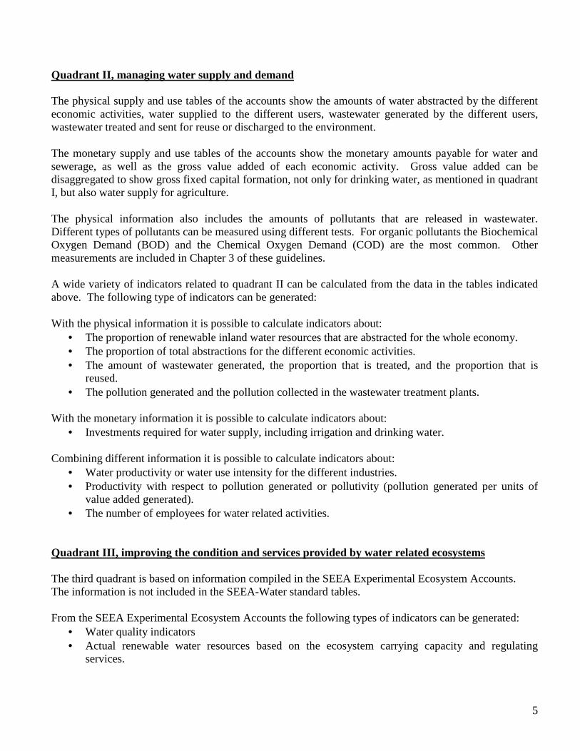
Water governance related information The information in the different quadrants described above will be useful for assessing water governance aspects. For example, all the financial information, the information about human resources required for the water sector and for water resources management provide the basis for informing about water governance. The SEEA provides a framework for coordinated work among the different institutions participating in water management activities. Core water tables The SEEA provides great flexibility in the compilation of water accounts in order to satisfy the needs of countries with different water problems and at different levels of development. Each country can decide which accounts and tables to compile according to its own priorities identified. However, some basic information may be common to most countries, so key elements of the accounts may be identified. These basic elements in the accounts are summarized in the core water tables. The core water tables aim to provide the minimum information to aid policy makers to make informed decisions. They provide both monetary and physical information in a combined presentation. As such, the core water tables give a succinct, policy relevant presentation. The core tables build upon the SEEA Central Framework, SEEA-Water, and the IRWS.
7
Table 4.1.1 SEEA core water table 1: combined physical and monetary table (preliminary)
Supply of water products (Currency units)
Natural water L.1.1 L.1.1 L.1.1 L.1.1 L.1.1 L.1.1 L.1.1 M.1.1.1-N.1.1.1L.1.1+M.1.1.1-
N.1.1.1
Sewerage services L.1.2 L.1.2 L.1.2 L.1.2 L.1.2 L.1.2 L.1.2 M.1.1.2-N.1.1.2L.1.2+M.1.1.2-
N.1.1.2
Natural water L.4 L.4 L.4 L.4 L.4 L.4 L.4 L.4 L.4 L.4Sewerage services L.5 L.5 L.5 L.5 L.5 L.5 L.5 L.5 L.5 L.5Other products
Use of water (Millions m3) E+G E+G E+G E+G E+G E+G E+G F.2+F.4 E+G+F.2+F.4Total Abstraction E E E E E E E E
G G G G G G G F.2+F.4 G G G+F.2+F.4Distributed water G.1+G.2 G.1+G.2 G.1+G.2 G.1+G.2 G.1+G.2 G.1+G.2 G.1+G.2 F.2 G.1+G.2 G.1+G.2 G.1+G.2+F.2Received wastewater G.3+G.4 G.3+G.4 G.3+G.4 G.3+G.4 G.3+G.4 G.3+G.4 G.3+G.4 F.4 G.3+G.4+F.4
F+H F+H F+H F+H F+H F+H F+H G.2+G.4 F+H+G2+G4F F F F F F F G.2+G.4 F+G2+G4
Distributed water/water for own use F.1+F.2 F.1+F.2 F.1+F.2 F.1+F.2 F.1+F.2 F.1+F.2 F.1+F.2 G.2 F.1+F.2+G.2Wastewater F.3.1+F.4.1 F.3.1+F.4.1 F.3.1+F.4.1 F.3.1+F.4.1 F.3.1+F.4.1 F.3.1+F.4.1 F.3.1+F.4.1 G.4.1 F.3.1+F.4.1+G.4.1Reused water F.3.2+F.4.2 F.3.2+F.4.2 F.3.2+F.4.2 F.3.2+F.4.2 F.3.2+F.4.2 F.3.2+F.4.2 F.3.2+F.4.2 G.4.2 F.3.2+F.4.2+G.4.2
H H H H H H H Hof which: losses I I I I I I I I
Water consumption (Millions m3)
P.1.1 P.1.1 P.1.1 P.1.1 P.1.1 P.1.1 P.1.1 P.1.1P.1.2 P.1.2 P.1.2 P.1.2 P.1.2 P.1.2 P.1.2 P.1.2O.1.1 O.1.1 O.1.1 O.1.1 O.1.1 O.1.1 O.1.1 O.1.1
O.1.2 O.1.2 O.1.2 O.1.2 O.1.2 O.1.2 O.1.2 O.1.2
To
tal
ISIC 01-03ISIC 05-33, 41-43
ISIC 36 ISIC 37ISIC
38,39, 45-99
Total industry
Hou
seho
lds
Gov
ern
me
nt
Total supply of productsIntermediate consumption and final use (Currency units)
Industries (by ISIC division)
Rest of the world
Taxes less subsidies on
products, trade and transport margins
ISIC 35
Actual final consumption
Gross value added (Currency units)Employment
Supply of water (Millions m3)Supply of water to other economic units
Use of water received from other economic units
Total returns
Gross fixed capital formation (Currency units)For water supplyFor sewerage/sanitation
Closing Stocks of fixed assets for water supply (Currency units)Closing Stocks of fixed assets for water sanitation (Currency units) Note 1: the codes in the tables are provided as an indication that the data items are in the IRWS. They may be to be revised. Note 2: The rows and columns highlighted in yellow show the information of most relevance to quadrant I.
8
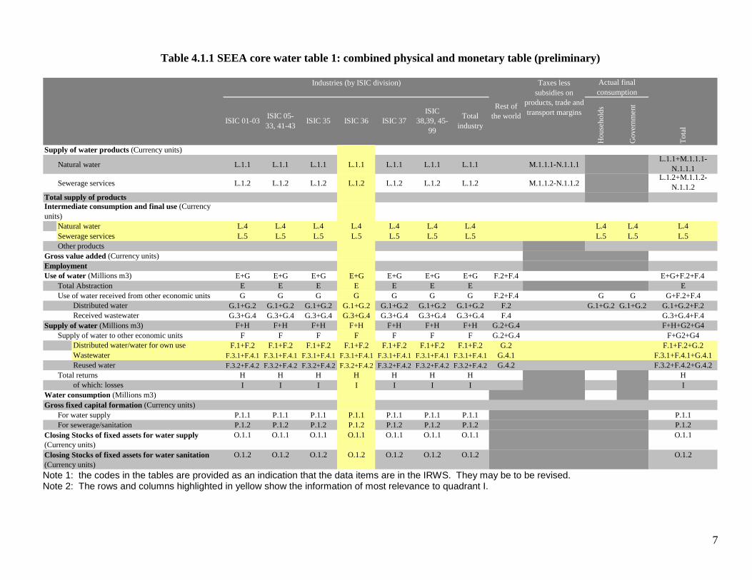
Table 4.1.2. SEEA core water table 2: water resources accounts (preliminary)
TotalSoil water
Artificial reservoirs
Lakes Rivers and
streams
Glaciers, snow and
ice
H.1.1.1 H.1.1.2 H.1.1.3 H.1.1.4 H.1.2 HB.1 B.1 B.1 B.1 B.1B.2 B.2 B.2 B.2 B.2 B.2
D.1 D
E.1.1.1 E.1.1.2 E.1.1.3 E.1.1.5 E.1.2 E.1.3 E.1of which for hydro power E.a.a
for cooling E.a.e
C.1 C.1 C.1 C.1 C.1C.2.1 C.2.1 C.2.1 C.2.1
C.2.2 C.2.2 C.2.2 C.2.2D.2 DOutflows to other inland water D.2
Abstraction
Evaporation & actual Outflows to other territoresOutflows to the sea
Inflows from other inland D.2Discoveries of water in
Reductions in stock
Additions to stockReturnsPrecipitationInflows from other territories
Type of water resourceSurface water Ground-
water
Note 1: the codes in the tables are provided as an indication that the data items are in the IRWS. They may be to be revised. Table 4.1.1 shows the SEEA core water table 1 highlighting the physical and monetary information directly related to the activities of water supply and sewerage, as well as the use of the products generated, namely natural water and sewerage services. Table 4.1.2 shows the SEEA core water table 2 with all the relevant information about the water cycle. REFERENCES: United Nations Statistics Division.- International Recommendations for Water Statistics.- 2012. United Nations Economic Commission for Europe. Making Data Meaningful: A Guide for Writing Stories About Numbers. UN 2009. ECE/CES/STAT/NONE/2009/4
9
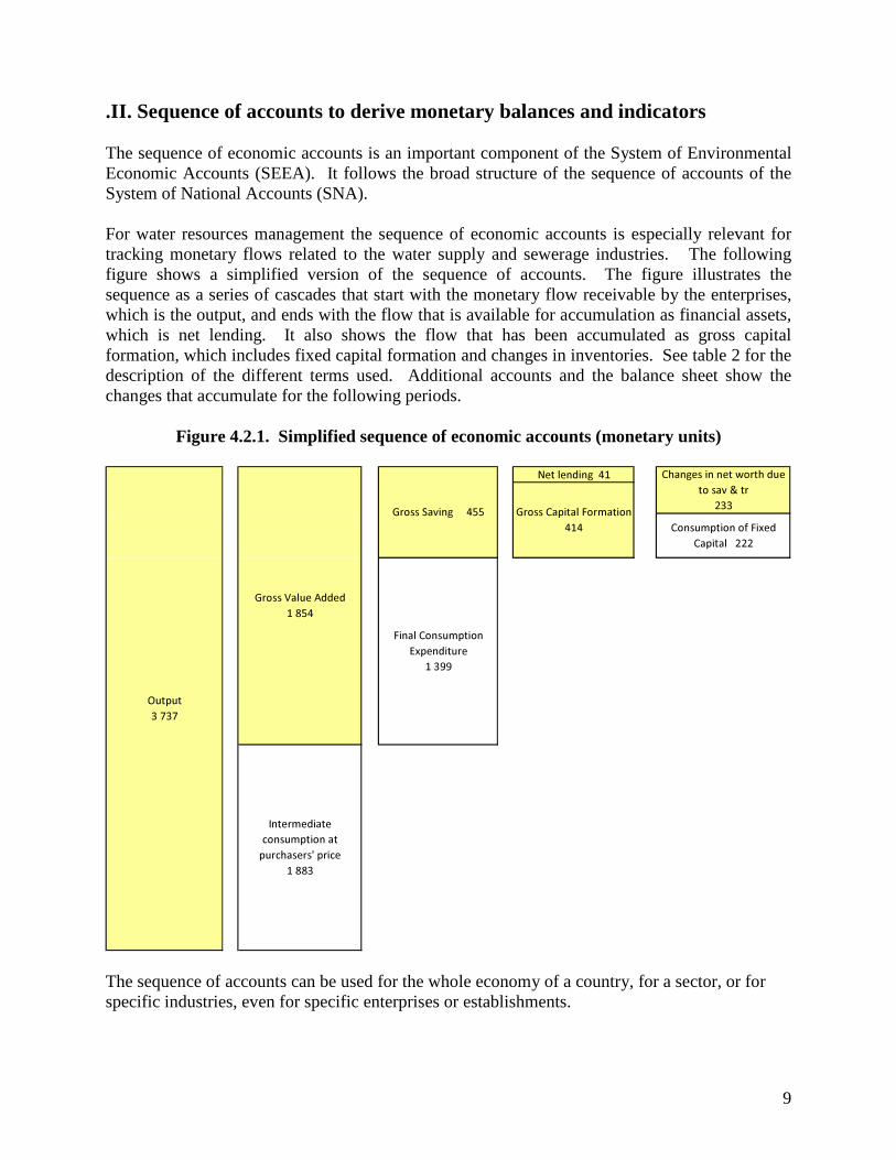
.II. Sequence of accounts to derive monetary balances and indicators The sequence of economic accounts is an important component of the System of Environmental Economic Accounts (SEEA). It follows the broad structure of the sequence of accounts of the System of National Accounts (SNA). For water resources management the sequence of economic accounts is especially relevant for tracking monetary flows related to the water supply and sewerage industries. The following figure shows a simplified version of the sequence of accounts. The figure illustrates the sequence as a series of cascades that start with the monetary flow receivable by the enterprises, which is the output, and ends with the flow that is available for accumulation as financial assets, which is net lending. It also shows the flow that has been accumulated as gross capital formation, which includes fixed capital formation and changes in inventories. See table 2 for the description of the different terms used. Additional accounts and the balance sheet show the changes that accumulate for the following periods.
Figure 4.2.1. Simplified sequence of economic accounts (monetary units)
Net lending 41
Consumption of Fixed
Capital 222
Changes in net worth due
to sav & tr
233Gross Capital Formation
414
Gross Value Added
1 854
Final Consumption
Expenditure
1 399
Gross Saving 455
Intermediate
consumption at
purchasers' price
1 883
Output
3 737
The sequence of accounts can be used for the whole economy of a country, for a sector, or for specific industries, even for specific enterprises or establishments.
10
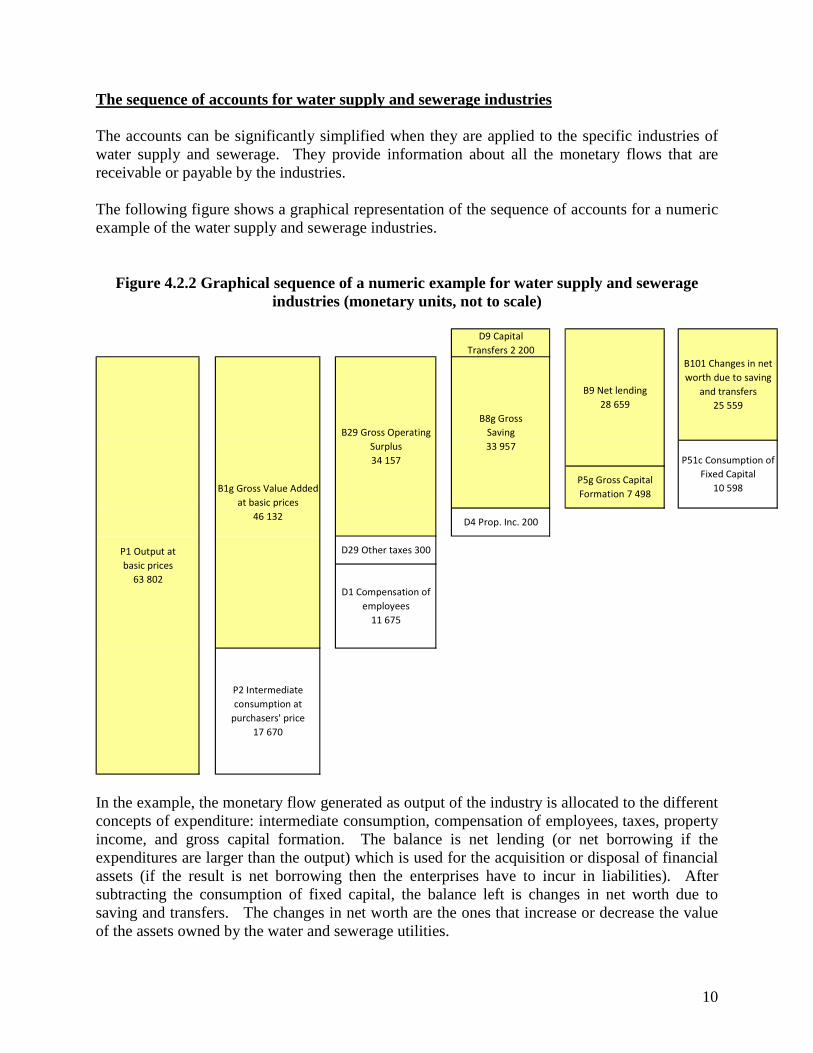
The sequence of accounts for water supply and sewerage industries The accounts can be significantly simplified when they are applied to the specific industries of water supply and sewerage. They provide information about all the monetary flows that are receivable or payable by the industries. The following figure shows a graphical representation of the sequence of accounts for a numeric example of the water supply and sewerage industries.
Figure 4.2.2 Graphical sequence of a numeric example for water supply and sewerage industries (monetary units, not to scale)
D4 Prop. Inc. 200
B9 Net lending
28 659
P5g Gross Capital
Formation 7 498
P51c Consumption of
Fixed Capital
10 598
B101 Changes in net
worth due to saving
and transfers
25 559
D9 Capital
Transfers 2 200
B29 Gross Operating
Surplus
34 157
B8g Gross
Saving
33 957
D29 Other taxes 300
D1 Compensation of
employees
11 675
B1g Gross Value Added
at basic prices
46 132
P2 Intermediate
consumption at
purchasers' price
17 670
P1 Output at
basic prices
63 802
In the example, the monetary flow generated as output of the industry is allocated to the different concepts of expenditure: intermediate consumption, compensation of employees, taxes, property income, and gross capital formation. The balance is net lending (or net borrowing if the expenditures are larger than the output) which is used for the acquisition or disposal of financial assets (if the result is net borrowing then the enterprises have to incur in liabilities). After subtracting the consumption of fixed capital, the balance left is changes in net worth due to saving and transfers. The changes in net worth are the ones that increase or decrease the value of the assets owned by the water and sewerage utilities.
11
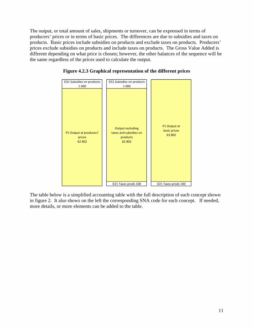
The output, or total amount of sales, shipments or turnover, can be expressed in terms of producers’ prices or in terms of basic prices. The differences are due to subsidies and taxes on products. Basic prices include subsidies on products and exclude taxes on products. Producers’ prices exclude subsidies on products and include taxes on products. The Gross Value Added is different depending on what price is chosen; however, the other balances of the sequence will be the same regardless of the prices used to calculate the output.
Figure 4.2.3 Graphical representation of the different prices
D21 Taxes prods 100 D21 Taxes prods 100
D31 Subsidies on products
1 000
D31 Subsidies on products
1 000
P1 Output at
basic prices
63 802P1 Output at producers'
prices
62 902
Output excluding
taxes and subsidies on
products
62 802
The table below is a simplified accounting table with the full description of each concept shown in figure 2. It also shows on the left the corresponding SNA code for each concept. If needed, more details, or more elements can be added to the table.

12
Table 4.2.1. Example of the sequence of accounts for water supply and sewerage industries (monetary units)
Receivable Payable Balance
P1 Output (producers' prices) 62 902
P2 Intermediate consumption 17 670
B1g Gross value added (producers' prices) 45 232
D1 Compensation of employees 11 675
D21 Taxes on products 100
D31 Subsidies on products -1000
D29 Other taxes on production 300
D39 Other subsidies on production
B2g Gross operating surplus 34 157
D4 Property income 0 200
B5g Balance of primary income 33 957
D5-D7 Current transfers 0 0 0
B8g Gross saving 33 957
P51c Consumption of fixed capital -10598 -10 598
D9 Capital transfers 2200
P51g Gross fixed capital formation 7 498
P52 Changes in inventories
B9 Net lending or borrowing 28 659
F Net acquisition of financial assets 0 28 659
F Net acquisition of liabilities
Zero balance 0 The changes in net worth will be calculated in the accumulation accounts, as will be shown below. Note that in the graph the concept of gross capital formation (P5g) is used. In the table, gross capital formation is disaggregated into gross fixed capital formation (P51g) and changes in inventories (P52). The following table presents a brief description of the terms used in the accounts. It is important to mention that the general principle in national accounting is that transactions between institutional units have to be recorded when claims and obligations arise, are transformed or are cancelled. This time of recording is called an accrual basis (SNA 2.56). For this reason the terms payable and receivable are used instead of the terms paid and received.
Table 4.2.2. Description of the concepts of the accounts Code Concept Description P1 Output at producers' prices
or at basic prices Amounts billed by the water supply and sewerage industries for the sales of water and sewerage. If it is at producers’ prices, it includes taxes and excludes

13
Code Concept Description subsidies on products. If it is at basic prices, it includes subsidies and excludes taxes on products. Note that output is calculated with the billed amounts (receivable) and not the actual amounts received. An important financial asset to observe is accounts receivable, which shows the billed amounts that were not paid during the current period.
P2 Intermediate consumption Amounts payable for the purchase of electricity, chemical products, water, administrative services, etc.
D1 Compensation of employees Amounts payable to people working in the industry for the concepts of wages and salaries, as well as the social contributions payable by the employers.
D21 Taxes on products Taxes directly applied to the price of water and sewerage
D29 Other taxes on production Taxes not directly applied to the price of water and sewerage.
D2 Taxes on production and imports
D21 + D29
D31 Subsidies on products Subsidies directly applied to the price of water and sewerage
D39 Other subsidies on production
Subsidies not directly applied to the price of water and sewerage.
D3 Subsidies D31 + D39 D4 Property income Property income includes several concepts, such as
payment of interests on loans, equity and dividends paid to the owners of the capital used. It also includes the payment of royalties, levies or duties for the use of water or the use of water bodies.
D5-D7
Current transfers Includes taxes on income, wealth, etc. It also includes net social contributions and social benefits.
P51c Consumption of fixed capital
It measures the depreciation of the equipment and infrastructure according to the criteria of the national accounts.
D9 Capital transfers Includes investment grants and other transfers for the acquisition of assets. Capital transfers are often large and irregular.
P51g Gross fixed capital formation
It includes the acquisition of fixed assets, such as pipes, pumps, buildings, and other infrastructure for the production of water and the provision of sewerage services. The disposals of fixed assets are subtracted from the acquisitions.
P52 Changes in inventories Changes in the amounts of goods that are purchased for production. The changes in the inventories of water are usually negligible, since the amounts of water stored in the systems owned by the utilities is relatively small.
14
Code Concept Description P5g Gross capital formation Gross capital formation includes gross fixed capital
formation, changes in inventories, and acquisition less disposal of valuables.
F Net acquisition of financial assets
Financial assets include currency and deposits, debt securities, equity and investment shares, financial derivatives, accounts receivable, etc.
F Net acquisition of financial liabilities
Financial liabilities include loans, accounts payable, etc.
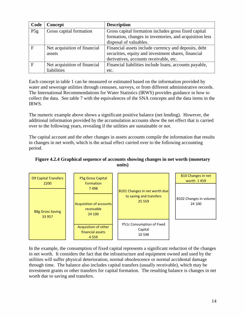
Each concept in table 1 can be measured or estimated based on the information provided by water and sewerage utilities through censuses, surveys, or from different administrative records. The International Recommendations for Water Statistics (IRWS) provides guidance in how to collect the data. See table 7 with the equivalences of the SNA concepts and the data items in the IRWS. The numeric example above shows a significant positive balance (net lending). However, the additional information provided by the accumulation accounts show the net effect that is carried over to the following years, revealing if the utilities are sustainable or not. The capital account and the other changes in assets accounts compile the information that results in changes in net worth, which is the actual effect carried over to the following accounting period.
Figure 4.2.4 Graphical sequence of accounts showing changes in net worth (monetary units)
B8g Gross Saving
33 957
D9 Capital Transfers
2200
B101 Changes in net worth due
to saving and transfers
25 559
P51c Consumption of Fixed
Capital
10 598
P5g Gross Capital
Formation
7 498
Acquisition of accounts
receivable
24 100
Acquisition of other
financial assets
4 559
B10 Changes in net
worth 1 459
B102 Changes in volume
24 100
In the example, the consumption of fixed capital represents a significant reduction of the changes in net worth. It considers the fact that the infrastructure and equipment owned and used by the utilities will suffer physical deterioration, normal obsolescence or normal accidental damage through time. The balance also includes capital transfers (usually receivable), which may be investment grants or other transfers for capital formation. The resulting balance is changes in net worth due to saving and transfers.
15
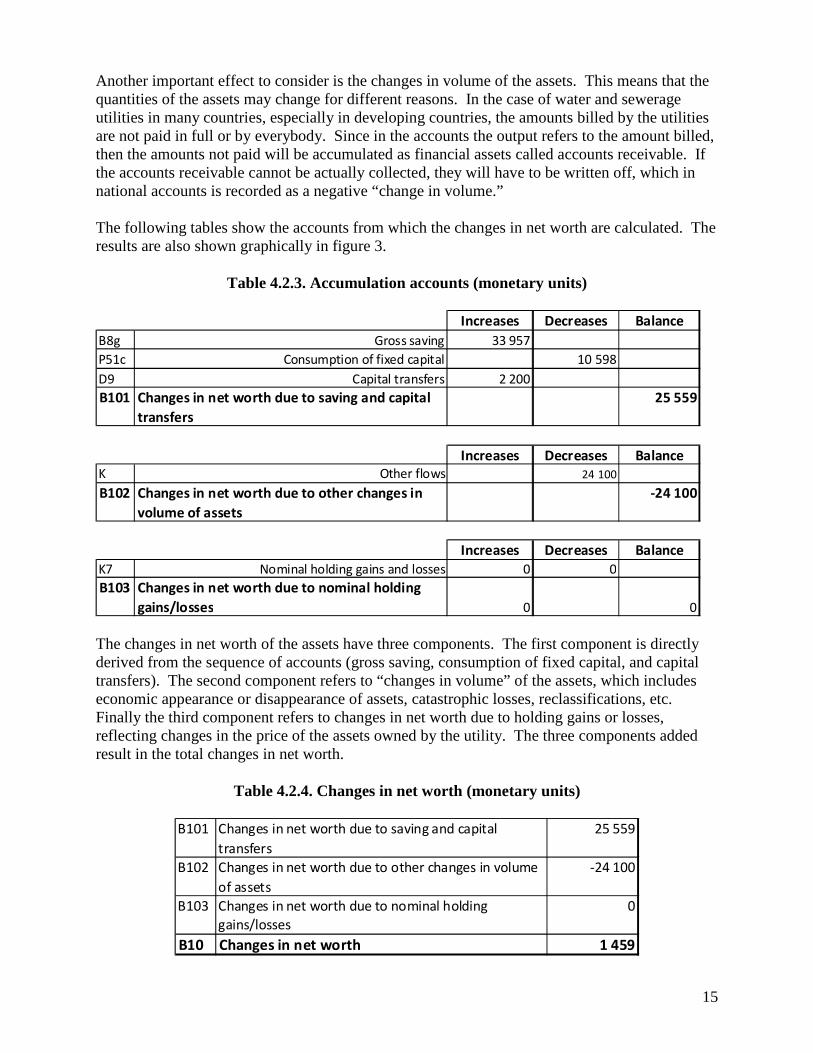
Another important effect to consider is the changes in volume of the assets. This means that the quantities of the assets may change for different reasons. In the case of water and sewerage utilities in many countries, especially in developing countries, the amounts billed by the utilities are not paid in full or by everybody. Since in the accounts the output refers to the amount billed, then the amounts not paid will be accumulated as financial assets called accounts receivable. If the accounts receivable cannot be actually collected, they will have to be written off, which in national accounts is recorded as a negative “change in volume.” The following tables show the accounts from which the changes in net worth are calculated. The results are also shown graphically in figure 3.
Table 4.2.3. Accumulation accounts (monetary units)
Increases Decreases Balance
B8g Gross saving 33 957
P51c Consumption of fixed capital 10 598
D9 Capital transfers 2 200
B101 Changes in net worth due to saving and capital
transfers
25 559
Increases Decreases Balance
K Other flows 24 100
B102 Changes in net worth due to other changes in
volume of assets
-24 100
Increases Decreases Balance
K7 Nominal holding gains and losses 0 0
B103 Changes in net worth due to nominal holding
gains/losses 0 0 The changes in net worth of the assets have three components. The first component is directly derived from the sequence of accounts (gross saving, consumption of fixed capital, and capital transfers). The second component refers to “changes in volume” of the assets, which includes economic appearance or disappearance of assets, catastrophic losses, reclassifications, etc. Finally the third component refers to changes in net worth due to holding gains or losses, reflecting changes in the price of the assets owned by the utility. The three components added result in the total changes in net worth.
Table 4.2.4. Changes in net worth (monetary units)
B101 Changes in net worth due to saving and capital
transfers
25 559
B102 Changes in net worth due to other changes in volume
of assets
-24 100
B103 Changes in net worth due to nominal holding
gains/losses
0
B10 Changes in net worth 1 459
16
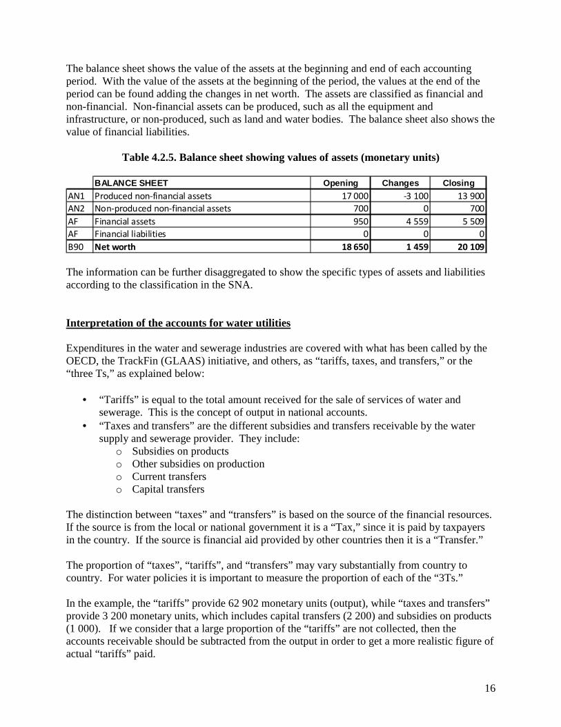
The balance sheet shows the value of the assets at the beginning and end of each accounting period. With the value of the assets at the beginning of the period, the values at the end of the period can be found adding the changes in net worth. The assets are classified as financial and non-financial. Non-financial assets can be produced, such as all the equipment and infrastructure, or non-produced, such as land and water bodies. The balance sheet also shows the value of financial liabilities.
Table 4.2.5. Balance sheet showing values of assets (monetary units)
BALANCE SHEET Opening Changes Closing
AN1 Produced non-financial assets 17 000 -3 100 13 900
AN2 Non-produced non-financial assets 700 0 700
AF Financial assets 950 4 559 5 509
AF Financial liabilities 0 0 0
B90 Net worth 18 650 1 459 20 109 The information can be further disaggregated to show the specific types of assets and liabilities according to the classification in the SNA. Interpretation of the accounts for water utilities Expenditures in the water and sewerage industries are covered with what has been called by the OECD, the TrackFin (GLAAS) initiative, and others, as “tariffs, taxes, and transfers,” or the “three Ts,” as explained below:
• “Tariffs” is equal to the total amount received for the sale of services of water and sewerage. This is the concept of output in national accounts.
• “Taxes and transfers” are the different subsidies and transfers receivable by the water supply and sewerage provider. They include:
o Subsidies on products o Other subsidies on production o Current transfers o Capital transfers
The distinction between “taxes” and “transfers” is based on the source of the financial resources. If the source is from the local or national government it is a “Tax,” since it is paid by taxpayers in the country. If the source is financial aid provided by other countries then it is a “Transfer.” The proportion of “taxes”, “tariffs”, and “transfers” may vary substantially from country to country. For water policies it is important to measure the proportion of each of the “3Ts.” In the example, the “tariffs” provide 62 902 monetary units (output), while “taxes and transfers” provide 3 200 monetary units, which includes capital transfers (2 200) and subsidies on products (1 000). If we consider that a large proportion of the “tariffs” are not collected, then the accounts receivable should be subtracted from the output in order to get a more realistic figure of actual “tariffs” paid.

17
The change in net worth shows if the assets own by the industry are being depleted or increased. If the change in net worth is positive, and everything remains the same, it means that the utility has enough financial resources to continue providing the services through the years to come. If the change in net worth is negative, it means that there is a financial gap that has to be covered with additional resources in order to avoid the depletion of the assets owned by the industry. Apparently a repayable loan can cover the financial gap; however, if the efficiencies are not increased, the gap will persist, since the loan has to be paid back, and the expenses will increase due to the interest on the loan. In the example above the change in net worth is positive. If the change in net worth were negative, then the assets of the industry would eventually be completely depleted. In the example there was a capital transfer of 2 200 monetary units. This could be an occasional investment grant. If that transfer is not received every year then the net worth will be negative for the years in which the grant is not received. Figure 4 shows a negative change in net worth (or gap) when the 2 200 monetary units are not included. There is a gap of 741 monetary units. The gap can be bridged by increasing the tariffs or subsidies, as well as by decreasing the expenses.
Figure 4.2.5 Financial gap if capital transfer is eliminated (monetary units, not to scale)
B10 Changes in net worth -741
B102 Changes in volume
24 100
B8g Gross Saving
33 957
P51c Consumption of
Fixed Capital
10 598
B101 Changes in net
worth due to saving
and transfers
23 359
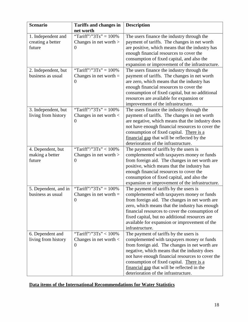
The example shows a significant change in net worth, 24 100 monetary units, due to changes in the volume of assets (i.e. the write off of the accounts receivable). This is because the utilities are unable to collect the amounts billed to its customers, reflecting what is known in water industries as a low commercial or administrative efficiency of the utility. The ratio of the amount of money actually collected and the amount billed is a common indicator of water utility performance. Scenarios of “tariffs” and changes in net worth The following table shows all the possible scenarios of “tariff” proportions (100% of expenditures covered by “tariffs,” or less than 100%) and changes in net worth (positive, zero, or negative). Table 4.2.6 Scenarios for different “tariff” propor tions and different values of the changes in net worth
18
Scenario Tariffs and changes in net worth
Description
1. Independent and creating a better future
“Tariff”/”3Ts” = 100% Changes in net worth > 0
The users finance the industry through the payment of tariffs. The changes in net worth are positive, which means that the industry has enough financial resources to cover the consumption of fixed capital, and also the expansion or improvement of the infrastructure.
2. Independent, but business as usual
“Tariff”/”3Ts” = 100% Changes in net worth = 0
The users finance the industry through the payment of tariffs. The changes in net worth are zero, which means that the industry has enough financial resources to cover the consumption of fixed capital, but no additional resources are available for expansion or improvement of the infrastructure.
3. Independent, but living from history
“Tariff”/”3Ts” = 100% Changes in net worth < 0
The users finance the industry through the payment of tariffs. The changes in net worth are negative, which means that the industry does not have enough financial resources to cover the consumption of fixed capital. There is a financial gap that will be reflected by the deterioration of the infrastructure.
4. Dependent, but making a better future
“Tariff”/”3Ts” < 100% Changes in net worth > 0
The payment of tariffs by the users is complemented with taxpayers money or funds from foreign aid. The changes in net worth are positive, which means that the industry has enough financial resources to cover the consumption of fixed capital, and also the expansion or improvement of the infrastructure.
5. Dependent, and in business as usual
“Tariff”/”3Ts” = 100% Changes in net worth = 0
The payment of tariffs by the users is complemented with taxpayers money or funds from foreign aid. The changes in net worth are zero, which means that the industry has enough financial resources to cover the consumption of fixed capital, but no additional resources are available for expansion or improvement of the infrastructure.
6. Dependent and living from history
“Tariff”/”3Ts” < 100% Changes in net worth < 0
The payment of tariffs by the users is complemented with taxpayers money or funds from foreign aid. The changes in net worth are negative, which means that the industry does not have enough financial resources to cover the consumption of fixed capital. There is a financial gap that will be reflected in the deterioration of the infrastructure.
Data items of the International Recommendations for Water Statistics
19
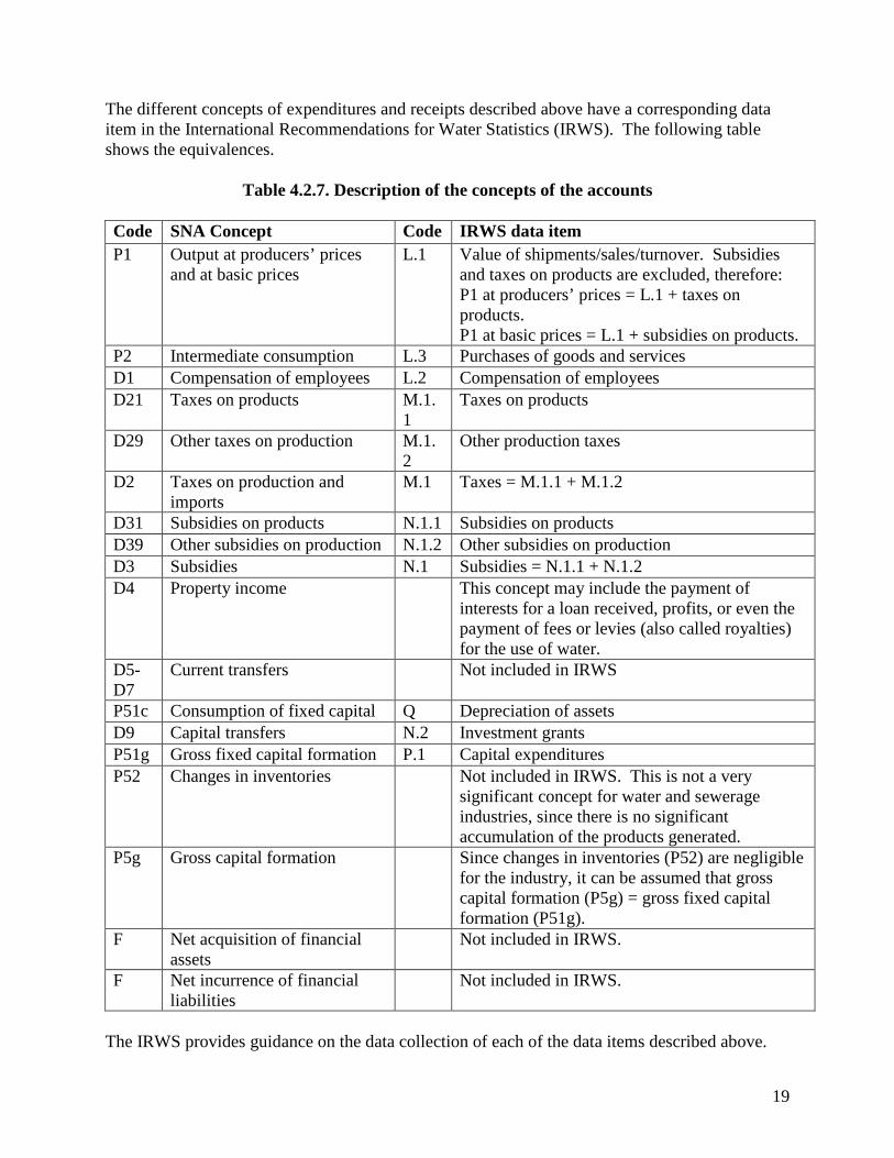
The different concepts of expenditures and receipts described above have a corresponding data item in the International Recommendations for Water Statistics (IRWS). The following table shows the equivalences.
Table 4.2.7. Description of the concepts of the accounts Code SNA Concept Code IRWS data item P1 Output at producers’ prices
and at basic prices L.1 Value of shipments/sales/turnover. Subsidies
and taxes on products are excluded, therefore: P1 at producers’ prices = L.1 + taxes on products. P1 at basic prices = L.1 + subsidies on products.
P2 Intermediate consumption L.3 Purchases of goods and services D1 Compensation of employees L.2 Compensation of employees D21 Taxes on products M.1.
1 Taxes on products
D29 Other taxes on production M.1.2
Other production taxes
D2 Taxes on production and imports
M.1 Taxes = M.1.1 + M.1.2
D31 Subsidies on products N.1.1 Subsidies on products D39 Other subsidies on production N.1.2 Other subsidies on production D3 Subsidies N.1 Subsidies = N.1.1 + N.1.2 D4 Property income This concept may include the payment of
interests for a loan received, profits, or even the payment of fees or levies (also called royalties) for the use of water.
D5-D7
Current transfers Not included in IRWS
P51c Consumption of fixed capital Q Depreciation of assets D9 Capital transfers N.2 Investment grants P51g Gross fixed capital formation P.1 Capital expenditures P52 Changes in inventories Not included in IRWS. This is not a very
significant concept for water and sewerage industries, since there is no significant accumulation of the products generated.
P5g Gross capital formation Since changes in inventories (P52) are negligible for the industry, it can be assumed that gross capital formation (P5g) = gross fixed capital formation (P51g).
F Net acquisition of financial assets
Not included in IRWS.
F Net incurrence of financial liabilities
Not included in IRWS.
The IRWS provides guidance on the data collection of each of the data items described above.

20
Sequence of flows instead of cascades Another way of illustrating the sequence of accounts, instead of the cascades shown in figures 4.2.1 to 4.2.4, is to use a sequence of flows, as shown in figure below. Figure 4.2.6. The sequence of accounts as a chain of flows The diagram in figure 4.2.5 shows the sequence of accounts starting from output (SNA code P1) and ending in the final balance, changes in net worth (SNA code B10). Most of the flows are
P2 Intermediate consumption
P1 Output (producers’ prices)
B.2 Inflows from neighboring territories
B1g Gross Value Added
D1 Compensation of employees
B2g Gross Operating Surplus
K Other flowsK Other flows
Net worth
B10 Changes in net worth (positive or negative)
D31 Subsidies on products
D21 Taxes on productsD29 Other taxes on production
D4 Property income
B8g Gross Saving
D5-D7 current transfers
B5g Balance of Primary Income
B101 Changes in net worth due to saving and capital transfers (positive or negative)
D9 capital transfers P51c Consumption of Fixed Capital
D31 Subsidies on products

21
connected to “clouds” since the diagram does not show the whole economy, but only one portion of it. The “clouds” show the flows that are generated or that go to parts of the economy that go beyond industries ISIC 36 and 37. Some flows may have a different direction depending on each specific case. For example, current transfers could flow from the utilities to other institutional units instead of the other way around. Current transfers could be income taxes, for example. The diagram ends with a box, which represents the stock of net worth. The stock of net worth is increased or decreased with the resulting balance of current flows. If the stock of net worth of the utility is consistently decreased, then in the long term the utility will collapse. Types of indicators derived from the sequence A list of different types of indicators that can be derived from the accounts is shown below. The formulas show the calculation of indicators using the codes in the SNA, shown in table 4.2.2. Economic sustainability Changes in net worth Balance B10 Expenditures, tariff level and collection efficiency Total expenditures (Opex + Capex) P2+D1+D29+D4+P51c Tariff level compared to expenditures P1/(P2+D1+D29+D4+P51c) Collection of fees efficiency (P1 – B102 of accounts receivable)/P1 REFERENCES: United Nations Economic Commission for Europe. Making Data Meaningful: A Guide for Writing Stories About Numbers. UN 2009. ECE/CES/STAT/NONE/2009/4
22
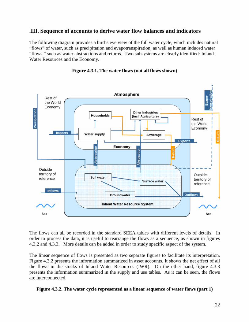
.III. Sequence of accounts to derive water flow balances and indicators The following diagram provides a bird’s eye view of the full water cycle, which includes natural “flows” of water, such as precipitation and evapotranspiration, as well as human induced water “flows,” such as water abstractions and returns. Two subsystems are clearly identified: Inland Water Resources and the Economy.
Figure 4.3.1. The water flows (not all flows shown)
Ab
stra
ctio
n
Imports
Exports
Pre
cip
itat
ion
EconomyEconomy
Water supply
HouseholdsOther industries
(incl. Agriculture)
Sewerage
Ret
urn
Rest ofthe World Economy
Rest ofthe World Economy
Eva
po
-tr
ansp
irat
ion
InlandInland WaterWater ResourceResource SystemSystem
Groundwater
Soil waterSurface water
OutflowsInflows
Outsideterritory ofreference
Outsideterritory ofreference
Sea
Ret
urn
Sea
Atmosphere
Ab
stra
ctio
n
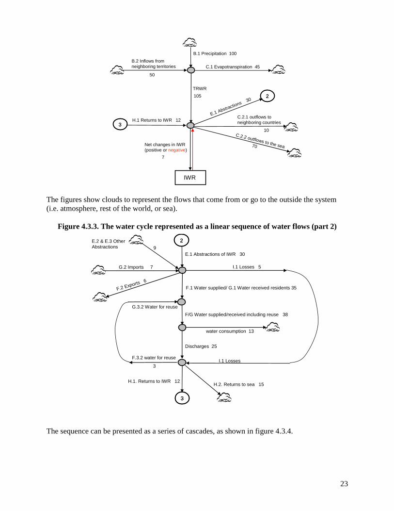
The flows can all be recorded in the standard SEEA tables with different levels of details. In order to process the data, it is useful to rearrange the flows as a sequence, as shown in figures 4.3.2 and 4.3.3. More details can be added in order to study specific aspect of the system. The linear sequence of flows is presented as two separate figures to facilitate its interpretation. Figure 4.3.2 presents the information summarized in asset accounts. It shows the net effect of all the flows in the stocks of Inland Water Resources (IWR). On the other hand, figure 4.3.3 presents the information summarized in the supply and use tables. As it can be seen, the flows are interconnected.
Figure 4.3.2. The water cycle represented as a linear sequence of water flows (part 1)
23
The figures show clouds to represent the flows that come from or go to the outside the system (i.e. atmosphere, rest of the world, or sea).
Figure 4.3.3. The water cycle represented as a linear sequence of water flows (part 2) The sequence can be presented as a series of cascades, as shown in figure 4.3.4.
3
water consumption 13
E.1 Abstractions of IWR 30
H.1. Returns to IWR 12
I.1 Losses 5
H.2. Returns to sea 15
G.2 Imports 7
F.2 Exports 6
9
G.3.2 Water for reuse
F.1 Water supplied/ G.1 Water received residents 35
Discharges 25
22
F.3.2 water for reuseI.1 Losses
33
E.2 & E.3 Other Abstractions
F/G Water supplied/received including reuse 38
C.1 Evapotranspiration 45
B.1 Precipitation 100
B.2 Inflows from neighboring territories
TRWR
E.1 Abstractions 30
22
IWR
Net changes in IWR (positive or negative)
H.1 Returns to IWR 12
C.2.2 outflows to the sea
C.2.1 outflows to neighboring countries 33
50
105
7
70
10
24
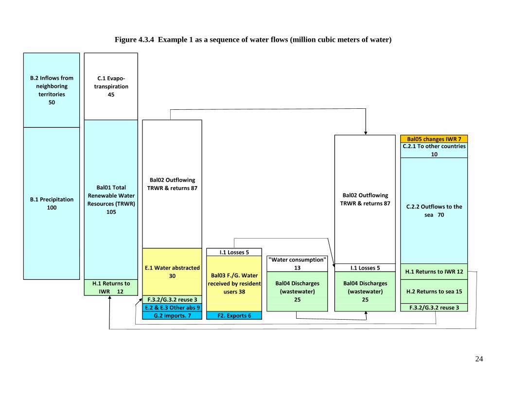
Figure 4.3.4 Example 1 as a sequence of water flows (million cubic meters of water)
Bal05 changes IWR 7
I.1 Losses 5
I.1 Losses 5
F.3.2/G.3.2 reuse 3
E.2 & E.3 Other abs 9 F.3.2/G.3.2 reuse 3
G.2 Imports. 7 F2. Exports 6
H.1 Returns to
IWR 12 H.2 Returns to sea 15
C.2.1 To other countries
10
C.2.2 Outflows to the
sea 70
E.1 Water abstracted
30 Bal03 F./G. Water
received by resident
users 38
"Water consumption"
13H.1 Returns to IWR 12
Bal04 Discharges
(wastewater)
25
Bal04 Discharges
(wastewater)
25
B.2 Inflows from
neighboring
territories
50
C.1 Evapo-
transpiration
45
Bal01 Total
Renewable Water
Resources (TRWR)
105
Bal02 Outflowing
TRWR & returns 87
B.1 Precipitation
100
Bal02 Outflowing
TRWR & returns 87

25
The information in figure 4 can be summarized in two sets of two columns. The first set shows one column with the additions and another column with the reductions in the stocks of inland water resources, as presented in the SEEA asset accounts. The second set shows one column with the supply of water in the economy and the other with the use of that water, as presented in the SEEA supply and use tables. Figure 4.3.5 two-bar summaries
Bal05 changes IWR 7
E.2 & E.3 Other ab 9
G.2 Imports. 7 F2. Exports 6
H.2 Returns to sea 15
H.1 Returns to
IWR 12
E.1 Water abstracted
30
E.1 Water abstracted
30
"Water consumption"
13
B.2 Inflows from
neighboring
territories
50
C.1 Evapo-transpiration
45
B.1 Precipitation
100
C.2.1 To other countries
10
C.2.2 Outflows to the
sea 70
H.1 Returns to
IWR 12 The information in figure 4 can also be presented in tables, which show the sequence of the cascades, each generating a balance, useful for the calculation of indicators. The tables show the different data items with their code according to the International Recommendations for Water Statistics.
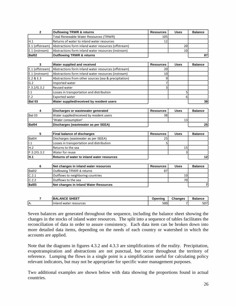
Table 4.3.3. Sequence of accounts for example 1
1 Renewable water Resources Uses BalanceB.1 Precipitation 100
B.2 Inflows from other territories 50
C.1 Evapotranspiration 45
Bal01 Total Renewable Water Resources (TRWR) 105
26
2 Ouflowing TRWR & returns Resources Uses Balance
Total Renewable Water Resources (TRWR) 105
H.1 Returns of water to inland water resources 12
E.1 (offstream) Abstractions form inland water resources (offstream) 20
E.1 (instream) Abstractions form inland water resources (instream) 10
Bal02 Outflowing TRWR & returns 87
3 Water supplied and received Resources Uses BalanceE.1 (offstream) Abstractions form inland water resources (offstream) 20
E.1 (instream) Abstractions form inland water resources (instream) 10
E.2 & E.3 Abstractions from other sources (sea & precipitation) 9
G.2 Imported water 7
F.3.2/G.3.2 Reused water 3
I.1 Losses in transportation and distribution 5
F.2 Exported water 6
Bal 03 Water supplied/received by resident users 38
4 Discharges or wastewater generated Resources Uses BalanceBal 03 Water supplied/received by resident users 38
"Water consumption" 13
Bal04 Discharges (wastewater as per SEEA) 25
5 Final balance of discharges Resources Uses BalanceBal04 Discharges (wastewater as per SEEA) 25
I.1 Losses in transportation and distribution 5
H.2 Returns to the sea 15
F.3.2/G.3.2 Water for reuse 3
H.1 Returns of water to inland water resources 12
6 Net changes in inland water resources Resources Uses BalanceBal02 Outflowing TRWR & returns 87
C.2.1 Outflows to neighboring countries 10
C.2.2 Outflows to the sea 70
Bal05 Net changes in Inland Water Resources 7
7 BALANCE SHEET Opening Changes BalanceA. Inland water resources 500 7 507 Seven balances are generated throughout the sequence, including the balance sheet showing the changes in the stocks of inland water resources. The split into a sequence of tables facilitates the reconciliation of data in order to assure consistency. Each data item can be broken down into more detailed data items, depending on the needs of each country or watershed in which the accounts are applied. Note that the diagrams in figures 4.3.2 and 4.3.3 are simplifications of the reality. Precipitation, evapotranspiration and abstractions are not punctual, but occur throughout the territory of reference. Lumping the flows in a single point is a simplification useful for calculating policy relevant indicators, but may not be appropriate for specific water management purposes. Two additional examples are shown below with data showing the proportions found in actual countries.
27
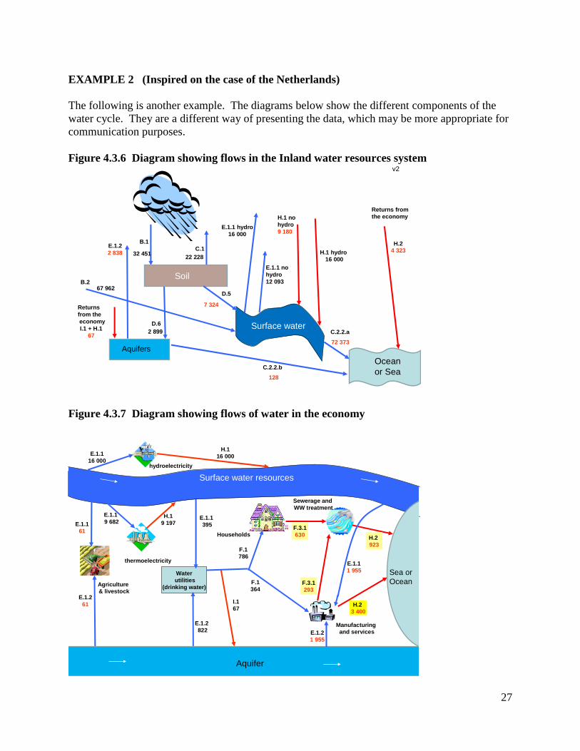
EXAMPLE 2 (Inspired on the case of the Netherlands) The following is another example. The diagrams below show the different components of the water cycle. They are a different way of presenting the data, which may be more appropriate for communication purposes. Figure 4.3.6 Diagram showing flows in the Inland water resources system
Surface water
Ocean or Sea
Aquifers
2 899
32 451
Soil
22 228
7 324
H.24 323
128
Returns from the economy
72 373
B.1C.1
D.5
D.6
E.1.1 hydro16 000
E.1.1 nohydro12 093
H.1 hydro 16 000
Returns from theeconomyI.1 + H.1
67
E.1.22 838
v2
B.267 962
H.1 nohydro9 180
C.2.2.a
C.2.2.b
Figure 4.3.7 Diagram showing flows of water in the economy
Surface water resources
Waterutilities
(drinking water)Agriculture & livestock
Households
Sewerage and WW treatment
Aquifer
E.1.161
E.1.2 822
F.1786
H.2 923
I.167
E.1.261
Manufacturing and services
E.1.1 395
F.1364
E.1.21 955
H.2 3 400
Sea or Ocean
E.1.116 000
H.116 000
hydroelectricity
E.1.11 955
F.3.1293
F.3.1630
thermoelectricity
E.1.1 9 682
H.19 197
28
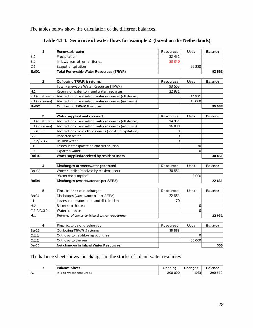
The tables below show the calculation of the different balances.
Table 4.3.4. Sequence of water flows for example 2 (based on the Netherlands)
1 Renewable water Resources Uses BalanceB.1 Precipitation 32 451
B.2 Inflows from other territories 83 340
C.1 Evapotranspiration 22 228
Bal01 Total Renewable Water Resources (TRWR) 93 563
2 Ouflowing TRWR & returns Resources Uses BalanceTotal Renewable Water Resources (TRWR) 93 563
H.1 Returns of water to inland water resources 22 931
E.1 (offstream) Abstractions form inland water resources (offstream) 14 931
E.1 (instream) Abstractions form inland water resources (instream) 16 000
Bal02 Outflowing TRWR & returns 85 563
3 Water supplied and received Resources Uses BalanceE.1 (offstream) Abstractions form inland water resources (offstream) 14 931
E.1 (instream) Abstractions form inland water resources (instream) 16 000
E.2 & E.3 Abstractions from other sources (sea & precipitation) 0
G.2 Imported water 0
F.3.2/G.3.2 Reused water 0
I.1 Losses in transportation and distribution 70
F.2 Exported water 0
Bal 03 Water supplied/received by resident users 30 861
4 Discharges or wastewater generated Resources Uses BalanceBal 03 Water supplied/received by resident users 30 861
"Water consumption" 8 000Bal04 Discharges (wastewater as per SEEA) 22 861
5 Final balance of discharges Resources Uses BalanceBal04 Discharges (wastewater as per SEEA) 22 861
I.1 Losses in transportation and distribution 70
H.2 Returns to the sea 0
F.3.2/G.3.2 Water for reuse 0
H.1 Returns of water to inland water resources 22 931
6 Final balance of discharges Resources Uses BalanceBal02 Outflowing TRWR & returns 85 563
C.2.1 Outflows to neighboring countries 0
C.2.2 Outflows to the sea 85 000
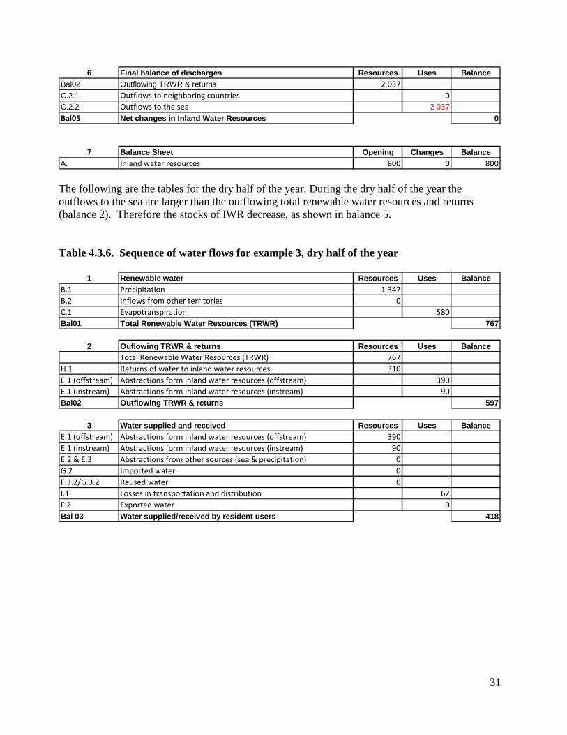
Bal05 Net changes in Inland Water Resources 563 The balance sheet shows the changes in the stocks of inland water resources.
7 Balance Sheet Opening Changes BalanceA. Inland water resources 200 000 563 200 563
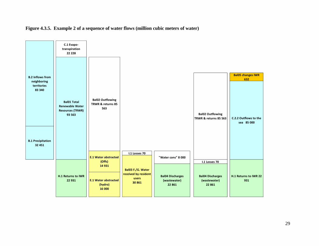
29
Figure 4.3.5. Example 2 of a sequence of water flows (million cubic meters of water)
I.1 Losses 70
I.1 Losses 70
C.2.2 Outflows to the
sea 85 000
H.1 Returns to IWR 22
931
H.1 Returns to IWR
22 931 E.1 Water abstracted
(hydro)
16 000
Bal03 F./G. Water
received by resident
users
30 861
Bal04 Discharges
(wastewater)
22 861
"Water cons" 8 000
Bal04 Discharges
(wastewater)
22 861
B.2 Inflows from
neighboring
territories
83 340
B.1 Precipitation
32 451
C.1 Evapo-
transpiration
22 228
Bal02 Outflowing
TRWR & returns 85 563
Bal02 Outflowing
TRWR & returns 85
563
Bal05 changes IWR
632
E.1 Water abstracted
(Offs)
14 931
Bal01 Total
Renewable Water
Resources (TRWR)
93 563

30
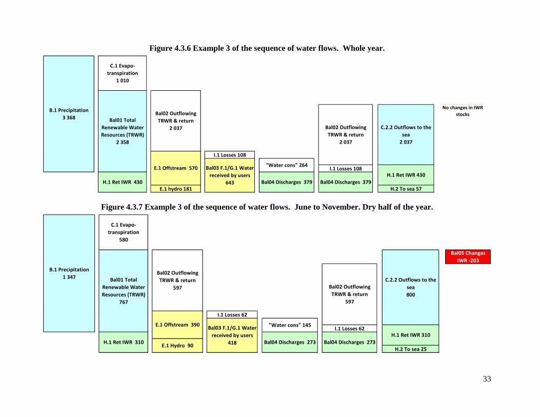
Example 3. (Inspired on the case of Mauritius) The following is another example showing the accounting tables and graphical sequence of accounts. The example shows the importance of time scale. If the accounts are for the whole year there is no apparent depletion of the stocks of inland water resources (IWR). However, when the accounts are only for the dry half of the year, there is a negative change in the stocks of inland water resources, which even if it happens for a short period of time, it has an important impact, especially in a country with a very limited stock of water. Table 4.3.5. Sequence of water flows for example 3, whole year
1 Renewable water Resources Uses BalanceB.1 Precipitation 3 368
B.2 Inflows from other territories 0
C.1 Evapotranspiration 1 010
Bal01 Total Renewable Water Resources (TRWR) 2 358
2 Ouflowing TRWR & returns Resources Uses BalanceTotal Renewable Water Resources (TRWR) 2 358
H.1 Returns of water to inland water resources 430
E.1 (offstream) Abstractions form inland water resources (offstream) 570
E.1 (instream) Abstractions form inland water resources (instream) 181
Bal02 Outflowing TRWR & returns 2 037
3 Water supplied and received Resources Uses BalanceE.1 (offstream) Abstractions form inland water resources (offstream) 570
E.1 (instream) Abstractions form inland water resources (instream) 181
E.2 & E.3 Abstractions from other sources (sea & precipitation) 0
G.2 Imported water 0
F.3.2/G.3.2 Reused water 0
I.1 Losses in transportation and distribution 108
F.2 Exported water 0
Bal 03 Water supplied/received by resident users 643
4 Discharges or wastewater generated Resources Uses BalanceBal 03 Water supplied/received by resident users 643
"Water consumption" 264
Bal04 Discharges (wastewater as per SEEA) 379
5 Final balance of discharges Resources Uses BalanceBal04 Discharges (wastewater as per SEEA) 379
I.1 Losses in transportation and distribution 108
H.2 Returns to the sea 57
F.3.2/G.3.2 Water for reuse 0
H.1 Returns of water to inland water resources 430
31
6 Final balance of discharges Resources Uses BalanceBal02 Outflowing TRWR & returns 2 037
C.2.1 Outflows to neighboring countries 0
C.2.2 Outflows to the sea 2 037
Bal05 Net changes in Inland Water Resources 0
7 Balance Sheet Opening Changes BalanceA. Inland water resources 800 0 800 The following are the tables for the dry half of the year. During the dry half of the year the outflows to the sea are larger than the outflowing total renewable water resources and returns (balance 2). Therefore the stocks of IWR decrease, as shown in balance 5. Table 4.3.6. Sequence of water flows for example 3, dry half of the year
1 Renewable water Resources Uses BalanceB.1 Precipitation 1 347
B.2 Inflows from other territories 0
C.1 Evapotranspiration 580
Bal01 Total Renewable Water Resources (TRWR) 767
2 Ouflowing TRWR & returns Resources Uses BalanceTotal Renewable Water Resources (TRWR) 767
H.1 Returns of water to inland water resources 310
E.1 (offstream) Abstractions form inland water resources (offstream) 390
E.1 (instream) Abstractions form inland water resources (instream) 90
Bal02 Outflowing TRWR & returns 597
3 Water supplied and received Resources Uses BalanceE.1 (offstream) Abstractions form inland water resources (offstream) 390
E.1 (instream) Abstractions form inland water resources (instream) 90
E.2 & E.3 Abstractions from other sources (sea & precipitation) 0
G.2 Imported water 0
F.3.2/G.3.2 Reused water 0
I.1 Losses in transportation and distribution 62
F.2 Exported water 0
Bal 03 Water supplied/received by resident users 418

32
4 Discharges or wastewater generated Resources Uses BalanceBal 03 Water supplied/received by resident users 418
"Water consumption" 145
Bal04 Discharges (wastewater as per SEEA) 273
5 Final balance of discharges Resources Uses BalanceBal04 Discharges (wastewater as per SEEA) 273
I.1 Losses in transportation and distribution 62
H.2 Returns to the sea 25
F.3.2/G.3.2 Water for reuse 0
H.1 Returns of water to inland water resources 310
6 Final balance of discharges Resources Uses BalanceBal02 Outflowing TRWR & returns 597
C.2.1 Outflows to neighboring countries 0
C.2.2 Outflows to the sea 800
Bal05 Net changes in Inland Water Resources - 203
7 Balance Sheet Opening Changes BalanceA. Inland water resources 800 - 203 597 The decrease in the stocks of IWR may not be a problem, if the stocks are sufficiently large and can be replenished in the wet part of the year. However, if the stocks are very limited, they will be completely depleted sometime during the dry period. The problem can be solved by increasing the storage capacity of the country, either by building more artificial reservoirs, or by increasing the natural capacity of the country to store water (e.g. protecting aquifer recharge areas, protecting wetlands, etc). It can also be solved by decreasing the abstractions of water, which can be achieved by reducing losses or by reducing the amount of water actually used in the different activities. Another solution is to change the patterns of abstractions, so that the returns (e.g from hydroelectric plants) can be used for other purposes.
33
Figure 4.3.6 Example 3 of the sequence of water flows. Whole year.
I.1 Losses 108
I.1 Losses 108
E.1 hydro 181 H.2 To sea 57
H.1 Ret IWR 430
No changes in IWR
stocksB.1 Precipitation
3 368
C.1 Evapo-
transpiration
1 010
Bal01 Total
Renewable Water
Resources (TRWR)
2 358
Bal02 Outflowing
TRWR & return
2 037
E.1 Offstream 570 Bal03 F.1/G.1 Water
received by users
643
"Water cons" 264
C.2.2 Outflows to the
sea
2 037
Bal04 Discharges 379 Bal04 Discharges 379
H.1 Ret IWR 430
Bal02 Outflowing
TRWR & return
2 037
Figure 4.3.7 Example 3 of the sequence of water flows. June to November. Dry half of the year.
I.1 Losses 62
I.1 Losses 62
H.2 To sea 25
Bal05 Changes
IWR -203
H.1 Ret IWR 310 Bal04 Discharges 273 Bal04 Discharges 273
H.1 Ret IWR 310
E.1 Hydro 90
E.1 Offstream 390
C.2.2 Outflows to the
sea
800
Bal02 Outflowing
TRWR & return
597
Bal03 F.1/G.1 Water
received by users
418
"Water cons" 145
B.1 Precipitation
1 347
C.1 Evapo-
transpiration
580
Bal01 Total
Renewable Water
Resources (TRWR)
767
Bal02 Outflowing
TRWR & return
597
D R A F T
34
Types of indicators derived from the sequence A list of different types of indicators that can be derived from the accounts is shown below. The formulas show the calculation of indicators using the codes of the data items of the IRWS. Natural endowments Total Renewable Water Resources (TRWR): Balance 01 Water dependency Indicators Dependency from other countries: (B.2 + G.2)/(Balance01 + G.2) Dependency from precipitation: B.1/Balance01 Dependency from alternate sources: (E.2 + E.3)/(Balance01 + E.2 + E.3) Water development Offstream abstractions as proportion of TRWR: E.1 (offstream)/Balance 01 Total abstractions as proportion of TRWR E.1/Balance01 Proportion of TRWR not outflowing (Balance01-Balance02)/Balance 01 Physical use efficiency Losses as a proportion of offstream abstractions: I.1/E.1(offstream) Reuse as a proportion of offstream water supplied F.3.2/(Balance 03 – E.1(instream) Wastewater treatment Proportion of point source polluting discharges treated H.a / Balance 04 from sewerage H.a. is a portion of H.1 and H.2 treated. These indicators can be divided by the total population or presented as a proportion of precipitation and inflows. Minimum set of data to be collected about the water cycle The tables, diagrams and indicators presented in the previous pages can be constructed with a limited number of data items. More details can be added for specific needs.

D R A F T
35
The International Recommendations for Water Statistics (IRWS) has a list of 400 data items. Only 17 of the 400 data items are needed to complete the sequence of accounts. In most cases only about 12 data items are actually required. The following table shows the data items that are collected through the different international questionnaires, such as, the OECD-Eurostat questionnaire, the UNSD-UNEP questionnaire, and the FAO Aquastat country surveys. Table 4.3.7. Data items needed for the sequence of accounts Num Data item with codes Collected by Remarks
1 B.1. Precipitation OECD, UNSD, Aquastat Statistics usually available. Need to be
integrated by geographical areas
2 B.2. Inflow of water from neighboring
territories
OECD, UNSD, Aquastat Usually only surface water data is available.
3 C.1. Evapotranspiration from inland water
resources
OECD, UNSD, Indirectly
collected by Aquastat
Estimated. May be presented as a
percentage of precipitation.
4 C.2.1. Outflow to neighbouring territories OECD, UNSD, Aquastat Usually only surface water
5 C.2.2. Outflow to the sea OECD, UNSD Usually only surface water
6 E.1. Abstractions from inland water resources OECD, UNSD, Aquastat Soil water excluded. Instream abstractions
(i.e. hydroelectricity and waterway locks)
are not collected. Important to separate
instream and offstream abstractions.
7 E.2. Collection of precipitation Not in questionnaires Not a substantial amount for most
countries.
8 E.3. Abstraction from the sea Not in questionnaires May be obtained from inventories of
desalination plants
9 F.1. Water supplied by resident economic
units to resident economic units
UNSD, OECD Abstractions less losses
10 F.2. Water exported to other territories
(water exports)
UNSD Not relevant for most countries
11 F.3.2. Water supplied for further use (reuse) OECD Water reuse. Same as G.3.2
12 G.2. Water imported by resident economic
units from the rest of the world (water
UNSD Not relevant for most countries
13 G.3.2. Water received for further use OECD Same as F.3.2
14 H.1. Returns to inland water resources Not in questionnaires Can be calculated based on discharges
(balance 04), which can be estimated from
abstractions and water consumption
coefficients.
15 H.2. Returns to the sea Not in questionnaires Only returns located near sea front. May
be estimated as a complement to H.1
16 I.1. Losses of water UNSD Unaccounted for water, drinking water and
agriculture
17 Water consumption Not in questionnaires Coefficients can be used for the different
industries.
D R A F T
36
A brief discussion about each of the data items follows: B.1. Precipitation Most countries routinely collect data about precipitation from several meteorological stations. It is important that National Statistics Offices work in partnership with meteorological offices to process the data and calculate the precipitation by geographical areas (i.e. country, regions, provinces, states, watersheds, etc.) by year, month and long term averages (e.g. normal precipitation). Monthly precipitation is very useful to understand seasonal variations and the possible need to compile sub-annual accounts. B.2. Inflow of water from neighboring territories Countries that share borders with other countries need to estimate the amount of water that enters the country (and leaves the country, data item C.2.1). Some countries may have established a bi-national committee to monitor the amount of water shared by the countries. Usually only surface water is measured, since subsurface water flows are more complicated to measure, but at least gross estimates should be made. C.1 Evapotranspiration This is the total amount of evaporation and transpiration that occurs in the country or territory. It may be estimated based on measurements of pan evaporation in climatological or meteorological stations, but it is difficult to determine. It may be easier to calculate it as a residual of precipitation less the reconstituted surface and groundwater runoff. It may be useful to separate the amount of evaporation that occurs in lakes and artificial reservoirs, which can be calculated with more precision. C.2.1 Outflows to neighboring territories See B.2. Inflow of water from neighboring territories C.2.2. Outflows to the sea Surface water flowing to the sea may be monitored using stream gages, and statistics can be processed for different time frames. Scarce data of subsurface water flowing to the sea may be available. E.1. Abstractions from inland water resources Abstractions can be estimated using administrative data (e.g. permit registries, abstraction fees payment records) or measurement for operations management (e.g. macro and micro metering by water utilities). It is important to collect the information by types or groups of industries, also by source (i.e. groundwater and surface water). It is also important to distinguish freshwater from brackish water, especially for industrial uses (e.g. cooling), even though there is no uniform criteria to make the distinction. E.2. Collection of precipitation It usually represents a small proportion of the amount of water used by households. It may be useful to collect data in areas where rainwater harvesting is common practice. E.3. Abstraction from the sea

D R A F T
37
They may be an important source of water, especially in arid areas. Statistics about the abstractions can be collected from inventories of desalination plants. F.1. Water supplied by resident economic units to resident economic units It can be calculated by subtracting losses to the abstractions or by measurements done at the point of use (e.g. micro-metering for billing of water utilities). It is important to disaggregate the data by industries or groups of industries, and households, receiving it. F.2. Water exported to other territories (water exports) Water exports are uncommon at international level (an exception is Israel water exports to Palestine), but may be common at sub-national level, where aqueducts are constructed for inter-basin transfers. There is usually operation management data for each aqueduct and reliable statistics can be compiled. F.3.2. Water supplied for further use (reuse) It is the amount of water reused: discharged by one establishment and supplied to another. Typical cases are from sewerage to agricultural fields, and also to other industries, such as thermoelectric plants for cooling. Statistics can be compiled with data from wastewater utilities. G.2. Water imported by resident economic units from the rest of the world (water imports) See above F.2. Water exported to other territories (water exports) G.3.2. Water received for further use See above F.3.2. Water supplied for further use (reuse) H.1. Returns to inland water resources Can be calculated based on discharges (balance 04), which is in turn estimated from abstractions and water consumption coefficients. It is complemented with H.2.Returns to the sea and F.3.2.Water supplied for further use. It is important to separate the returns from the different type of uses (e.g. instream and offstream, by industry). Returns from wastewater treatment plants are especially relevant for estimating emissions. H.2. Returns to the sea This is the portion of water discharged directly to the sea. It is relevant for industries and households located by the sea. I.1. Losses of water Losses are relevant in drinking water supply networks, where losses can be as high as 50% of the water injected in the network. They are also relevant in aqueducts, especially open channels, for conveying water to agricultural fields, where losses can also be as high as 50% of the water abstracted. Water consumption Water consumption can be estimated using coefficients for the different types of industries and for households. Detailed explanations about the collection of each data item are found in chapter 3 of the Guidelines for the Compilation of Water Accounts and Statistics.

D R A F T
38
Emissions Emissions are waterborne substances in returns to inland water resources. Emissions are linked to discharges (balance 04 in the sequence above). Wastewater treatment plants remove some of the emissions from discharges before water is returned to inland water resources (data item H.1) or to the sea (data item H.2). Additional indicators derived from emission accounts Organic pollution generated and removed Organic pollution discharged by the economy J (based on BOD or COD) Organic pollution removed by WWTP J - K.1 (based on BOD or COD) WWTP = wastewater treatment plants Minimum set of data to be collected about emissions
Table 4.3.8 Data items needed for emission accounts Num Data item with codes Collected by Remarks
1 J. Waterborne polluting discharges Not in questionnaires At least total amount of BOD or COD
should be estimated.
2 K.1 Waterborne emissions from point sources Not in questionnaires BOD and COD emissions may be estimated
from inventories of wastewater treatment
plants, as well as from estimates of
wastewater collected by sewerage, and
discharges by industries.
3 K.2 Waterborne emissions from non-point
sources
Not in questionnaires Estimates of nitrates and phosphates could
be made based on sales of fertilizers.
J. Waterborne polluting discharges The polluting discharges in terms of the biochemical oxygen demand (BOD) or the chemical oxygen demand (COD) can be estimated using population data and the polluting discharges per person, as well as the polluting discharges based on the different types of industries. Wastewater utilities can provide additional information for the estimates. K.1. Waterborne emissions from point sources BOD and COD emissions may be estimated from inventories of wastewater treatment plants, based on data from wastewater plant operators, who need to have plant inflows and ouflow data. Also estimates of total amount of wastewater collected by sewerage and pollution concentrations, as well as discharges by industries.

D R A F T
39
REFERENCES: United Nations Economic Commission for Europe. Making Data Meaningful: A Guide for Writing Stories About Numbers. UN 2009. ECE/CES/STAT/NONE/2009/4
Recommended