Chapter 3 ESTIMATING ABUNDANCE AND DENSITY:
ADDITIONAL METHODS (Version 4, 14 March 2013) Page
3.1 EXPLOITED POPULATION TECHNIQUES ....................................................... 91
3.1.1 Change-in-Ratio Methods ..................................................................... 91
3.1.2 Planning Change-in-Ratio Studies ...................................................... 96
3.1.3 Eberhardt’s Removal Method ............................................................. 100
3.1.4 Catch-Effort Methods .......................................................................... 103
3.2 RESIGHT METHODS........................................................................................ 109
3.3 ENUMERATION METHODS ............................................................................ 116
3.4 ESTIMATING DENSITY ................................................................................... 118
3.4.1 Boundary Strip Methods .................................................................... 119
3.4.2 Nested Grids Method.......................................................................... 123
3.4.3 Spatial Methods for Multiple Recaptures ......................................... 125
3.5 SUMMARY ....................................................................................................... 130
SELECTED READING ........................................................................................... 131
QUESTIONS AND PROBLEMS ............................................................................. 132
Several methods have been developed for population estimation in which the
organisms need to be captured only one time. The first set of these were developed
for exploited populations in which the individuals were removed as a harvest from the
population, and they are loosely described as removal methods. These methods
were first developed in the 1940s for wildlife and fisheries management to get
estimates of the population under harvest. A discussion of removal methods forms
the first section of this chapter.
A second set of methods are of much more recent development and are based
on the principle of resighting animals that have been marked. They require an
individual animal to be captured only once, and then all subsequent “recaptures” are
Chapter 3 Page 91
from sighting records only - the individual never has to be physically captured again.
These newer methods were developed for animals with radio-collars but can be use
for any kind of mark which is visible to a distant observer. We shall discuss these
resighting methods in the second section of this chapter.
Mark-recapture methods have developed into very complex statistical methods
during the last 10 years. While many of these methods are beyond the scope of this
book, we can still use these methods for field populations once we understand their
assumptions. In the third section of this chapter I will provide an overview of how we
can convert abundance estimates to density estimates.
3.1 EXPLOITED POPULATION TECHNIQUES A special set of techniques have been developed for estimating population size in
exploited populations. Many of these techniques are highly specific for exploited fish
populations (Ricker 1975, Seber 1982) but some are of general interest because they
can be applied to wildlife and fisheries problems as well as other field situations. I will
briefly describe two types of approaches to population estimation that can be used
with exploited populations.
3.1.1 Change-in-Ratio Methods
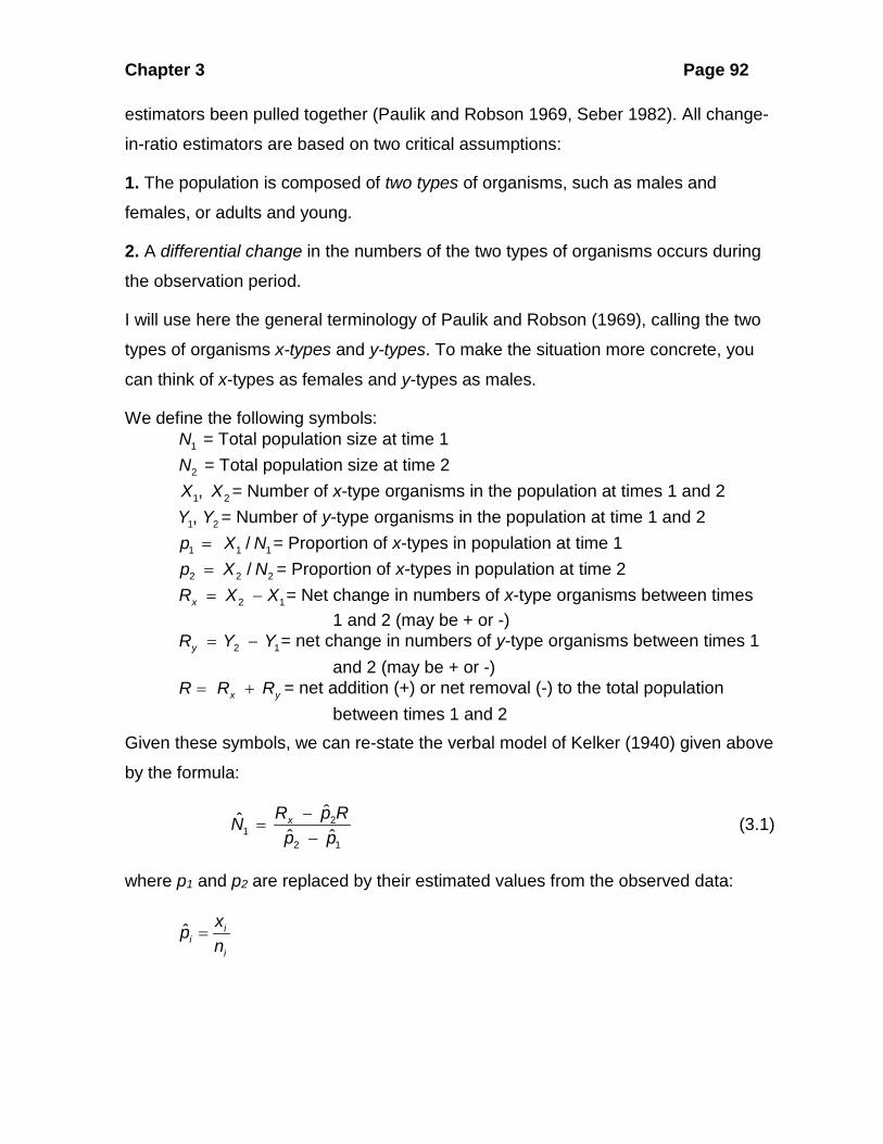
The idea that population size could be estimated from field data on the change in sex
ratio during a hunting season was first noted by Kelker (1940). When only one sex is
hunted, and the sex ratio before and after hunting is known, as well as the total kill,
Kelker showed that one could calculate a population estimation from the simple ratio:
Fraction of males Number of males befor Number of males -
in population hunting removed = Total number ofafter hunting
Total population size - aremovals
before hunting season
nimals killed
by hunters
Several investigators discovered and rediscovered this approach during the last 50
years (Hanson 1963), and only recently has the general theory of change-in-ratio
Chapter 3 Page 92
estimators been pulled together (Paulik and Robson 1969, Seber 1982). All change-
in-ratio estimators are based on two critical assumptions:
1. The population is composed of two types of organisms, such as males and
females, or adults and young.
2. A differential change in the numbers of the two types of organisms occurs during
the observation period.
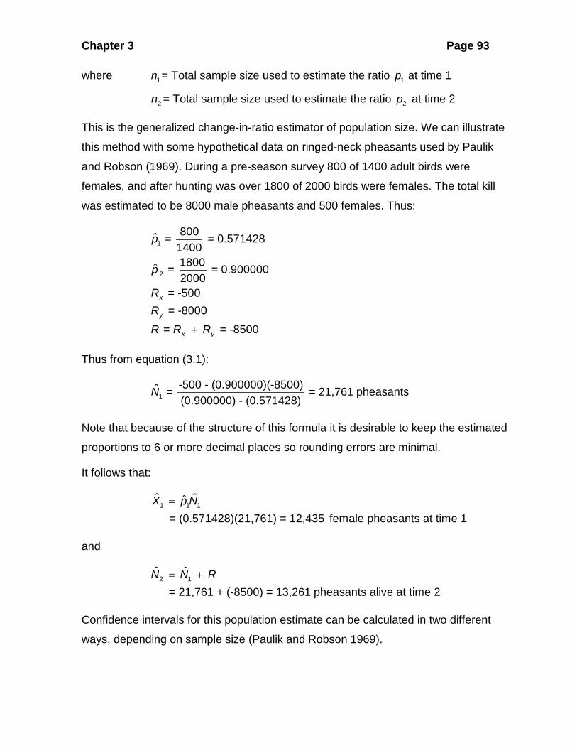
I will use here the general terminology of Paulik and Robson (1969), calling the two
types of organisms x-types and y-types. To make the situation more concrete, you
can think of x-types as females and y-types as males.
We define the following symbols: 1N = Total population size at time 1 2N = Total population size at time 2 1 2,X X = Number of x-type organisms in the population at times 1 and 2 1 2,Y Y = Number of y-type organisms in the population at time 1 and 2 1 1 1/p X N= = Proportion of x-types in population at time 1 2 2 2/p X N= = Proportion of x-types in population at time 2 2 1xR X X= − = Net change in numbers of x-type organisms between times 1 and 2 (may be + or -) 2 1yR Y Y= − = net change in numbers of y-type organisms between times 1 and 2 (may be + or -) x yR R R= + = net addition (+) or net removal (-) to the total population between times 1 and 2 Given these symbols, we can re-state the verbal model of Kelker (1940) given above
by the formula:
21
2 1
ˆˆˆ ˆxR p RNp p
−=
− (3.1)
where p1 and p2 are replaced by their estimated values from the observed data:
ˆ ii
i
xpn
=
Chapter 3 Page 93
where 1n = Total sample size used to estimate the ratio 1p at time 1
2n = Total sample size used to estimate the ratio 2p at time 2
This is the generalized change-in-ratio estimator of population size. We can illustrate
this method with some hypothetical data on ringed-neck pheasants used by Paulik
and Robson (1969). During a pre-season survey 800 of 1400 adult birds were
females, and after hunting was over 1800 of 2000 birds were females. The total kill
was estimated to be 8000 male pheasants and 500 females. Thus:
1
2
800ˆ = = 0.57142814001800ˆ = = 0.9000002000
= -500 = -8000
= = -8500
x
y
x y
p
p
RR
R R R+
Thus from equation (3.1):
1-500 - (0.900000)(-8500)ˆ = = 21,761 pheasants(0.900000) - (0.571428)
N
Note that because of the structure of this formula it is desirable to keep the estimated
proportions to 6 or more decimal places so rounding errors are minimal.
It follows that:
1 1 1ˆ ˆˆ
= (0.571428)(21,761) = 12,435 female pheasants at time 1X p N=
and
2 1ˆ ˆ
= 21,761 + (-8500) = 13,261 pheasants alive at time 2N N R= +
Confidence intervals for this population estimate can be calculated in two different
ways, depending on sample size (Paulik and Robson 1969).

Chapter 3 Page 94
Large samples: when approximately 500 or more individuals are sampled to
estimate 1p and an equal large number to estimate 2p , you should use the normal
approximation:
( ) ( ) ( )2 21 1 2 2
1 21 2
ˆ ˆˆ ˆ variance( ) variance( )ˆVariance ˆ ˆ( )
N p N pN
p p+
=−
(3.2)
1 11
1
ˆ ˆ(1 )ˆwhere Variance( ) p ppn−
= (3.3)
2 22
2
ˆ ˆ(1 )ˆVariance( ) p ppn−
= (3.4)
This variance formula assumes binomial sampling with replacement and is a
reasonable approximation to sampling without replacement when less than 10% of
the population is sampled (Seber 1982 p. 356). It also assumes that xR and yR (the
removals) are known exactly with no error.
For the pheasant example above:
1
2
(0.571428)(1 - 0.571428)ˆVariance of = = 0.00017491400
(0.9)(1 - 0.9)ˆVariance of = = 0.0000452000
p
p
Thus:
( )2 2
1 2(21,761) (0.0001749) + (13,261) (0.000045)ˆVariance =
(0.900000 - 0.571428) = 840,466
N
The standard error is given by:
1 1ˆ ˆStandard error of = Variance( )
= 840,446 916.8
N N
=
The 95% confidence limits follow from the normal distribution:
1 1ˆ ˆ 1.96[S.E.( )]N N±
Chapter 3 Page 95
For these data:
21,761 1.96(916.8)±
or 19,964 to 23,558 pheasants.
Small samples: When less than 100 or 200 individuals are sampled to estimate 1p
and 2p , you should use an alternative method suggested by Paulik and Robson
(1969). This method obtains a confidence interval for the reciprocal of 1N as follows:
21
1 4 22 12 2
Variance Varianceˆ( ) 1ˆVariance of (1/ ) = ˆ ˆˆ of of ( ) ( )x
x x
R p RNp pR p R R p R
−= − −
(3.5)
where variance of 1p = as defined in equation (3.3)
variance of 2p = as defined in equation (3.4)
and all other terms are as defined above (page 92).
This formula assumes that xR and yR are known without error. If we apply this
formula to the pheasant data used above:
2
1 4
2
[-8000 - (0.428571)(-8500)]ˆVariance of (1/ ) = (0.000045)[ 8000 - (0.10)(-8500)]
1 + (0.0001749)[-8000 - (0.10)(-8500)]
= 3.7481 X
N−
-12
1 1
-12 -6
10ˆ ˆStandard error of (1/ ) = Variance(1/ )
= 3.7481 x 10 = 1.9360 x 10
N N
The 95% confidence interval is thus:
11
-6
1 ˆ1.96 [S.E.(1/ )]ˆ
1 1.96 (1.9360 x 10 )21,761
NN
±
±
or 4.2159 x 510− to 4.9748 x 510−
Chapter 3 Page 96
Inverting these limits to get confidence limits for 1N :
-5
-5
1Lower 95% confidence limit = = 20,101 pheasants4.9748 x 10
1Upper 95% confidence limit = 23,720 pheasants4.2159 x 10
=
Note that these confidence limits are asymmetrical about 1N and are slightly wider
than those calculated above using the (more appropriate) large sample formulas on
these data.
The program RECAP (Appendix 2, page 000) can do these calculations for the
generalized change-in-ratio estimator of population size.
3.1.2 Planning Change-in-Ratio Studies
If you propose to use the change-in-ratio estimator (eq. 3.1) to estimate population
size, you should use the approach outlined by Paulik and Robson (1969) to help plan
your experiment. Five variables must be guessed at to do this planning:
1. 1 2 = p p p∆ = − Expected change in the proportion of x-types during the experiment
2. 1Rate of exploitation = /u R N= , which is the fraction of the whole population that is removed
3. /xf R R= = fraction of x-types in the removals
4. Acceptable limits of error for the 1N estimate (± 25% might be usual) see page 000)
5. Probability (1 α− ) of achieving the acceptable limits of error defined in (4); 90% or 95% might be the usual values here.
Figure 3.1 shows the sample sizes required for each sample ( 1 2,n n ) for
combinations of these parameters with the limits of error set at ±25% and (1 α− ) as
90%. To use Figure 3.1, proceed as follows:
1. Estimate two of the three variables plotted - the change in proportion of x-types, the rate of exploitation, and the fraction of x-types in the removal.
2. From these two variables, locate your position on the graph in Figure 3.1, and read the nearest contour line to get the sample size required for each sample.

Chapter 3 Page 97
For example, if 60% of the whole population will be harvested and you expect 75% of
the harvested animals to be x-types, Figure 3.1 shows that sample size should be
about 100 for the first sample and 100 for the second sample (to achieve error limits
of ±25% with a 1 α− of 0.90).
Figure 3.1 Sample sizes required for change-in-ratio estimation of population size with
acceptable error limits of ± 25 % with (1 - α) of 0.90 when the initial proportion of x-
types is 0.50. The contour lines represent the sample sizes needed in each of the time
1 and time 2 samples. The required sample sizes are only slightly affected by changes
in the rate of exploitation (u) but are greatly affected by changes in p∆ . (Source:
Paulik and Robson, 1969).
Two general points can be noted by inspecting Figure 3.1, and we can formulate
them as rules of guidance:
1. p∆ , the expected change in proportions, is the critical variable affecting the required sample sizes of change-in-ratio experiments. The rate of exploitation (u) is of minor importance, as is the fraction of x-types in the removals (f).
2. For p∆ less than 0.05, this method requires enormous sample sizes and in practice is not useful for field studies. If p is less than 0.10, large sample sizes
Chapter 3 Page 98
are needed and it is especially critical to test all the assumptions of this approach.
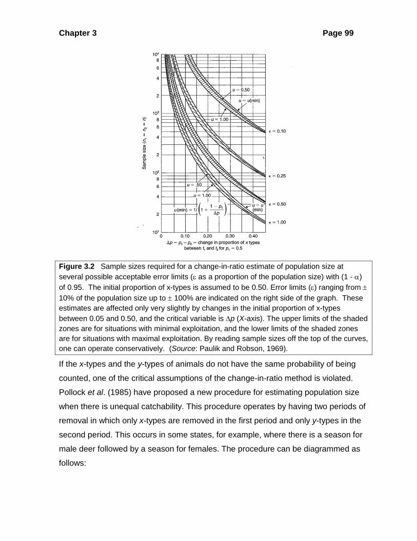
Using a series of graphs like Figure 3.1, Paulik and Robson (1969) synthesized
Figure 3.2 from which one can read directly the required sample sizes for change-in-
ratio experiments. We can illustrate the utility of this graph with an example.
Suppose you are planning a change-in-ratio experiment for a deer population
and you expect a change in the sex-ratio by at least 0.30 over the hunting season. If
you desire to estimate population size with an accuracy of ± 25%, from Figure 3.2
you can estimate the necessary sample size to be approximately 200-250 deer to be
sexed in both the before-hunting sample and the after-hunting sample. If you want ±
10% accuracy, you must pay for it by increasing the sample size to 1050-1400 deer
in each sample. Clearly, if your budget will allow you to count and sex only 40 deer in
each sample, you will get an estimate of N1 accurate only to ± 100%. If this is
inadequate, you need to reformulate your research goals.
Figures 3.1 and 3.2 are similar in general approach to Figures 2.3 and 2.4
(page 000) which allow one to estimate samples required in a Petersen-type mark-
recapture experiment. Paulik and Robson (1969) show that Petersen-type marking
studies can be viewed as a special case of a change-in-ratio estimator in which x-
type animals are marked and y-type unmarked.
All the above methods for change-in-ratio estimation are designed for closed
populations and are based on the assumption that all individuals have an equal
chance of being sampled in both the first and in the second samples. Seber (1982,
Chapter 9) discusses more complex situations for open populations and techniques
for testing the assumptions of this method.
Chapter 3 Page 99
Figure 3.2 Sample sizes required for a change-in-ratio estimate of population size at several possible acceptable error limits (ε as a proportion of the population size) with (1 - α) of 0.95. The initial proportion of x-types is assumed to be 0.50. Error limits (ε) ranging from ± 10% of the population size up to ± 100% are indicated on the right side of the graph. These estimates are affected only very slightly by changes in the initial proportion of x-types between 0.05 and 0.50, and the critical variable is ∆p (X-axis). The upper limits of the shaded zones are for situations with minimal exploitation, and the lower limits of the shaded zones are for situations with maximal exploitation. By reading sample sizes off the top of the curves, one can operate conservatively. (Source: Paulik and Robson, 1969).
If the x-types and the y-types of animals do not have the same probability of being
counted, one of the critical assumptions of the change-in-ratio method is violated.
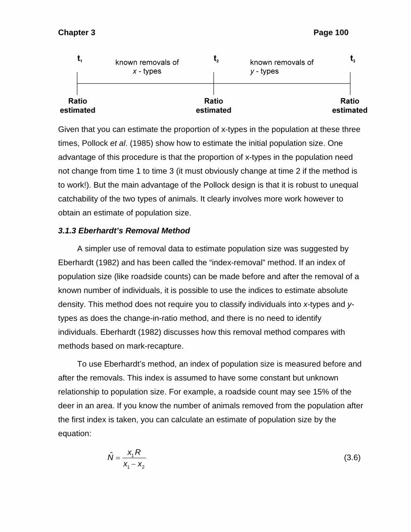
Pollock et al. (1985) have proposed a new procedure for estimating population size
when there is unequal catchability. This procedure operates by having two periods of
removal in which only x-types are removed in the first period and only y-types in the
second period. This occurs in some states, for example, where there is a season for
male deer followed by a season for females. The procedure can be diagrammed as
follows:
Chapter 3 Page 100
Given that you can estimate the proportion of x-types in the population at these three
times, Pollock et al. (1985) show how to estimate the initial population size. One
advantage of this procedure is that the proportion of x-types in the population need
not change from time 1 to time 3 (it must obviously change at time 2 if the method is
to work!). But the main advantage of the Pollock design is that it is robust to unequal
catchability of the two types of animals. It clearly involves more work however to
obtain an estimate of population size.
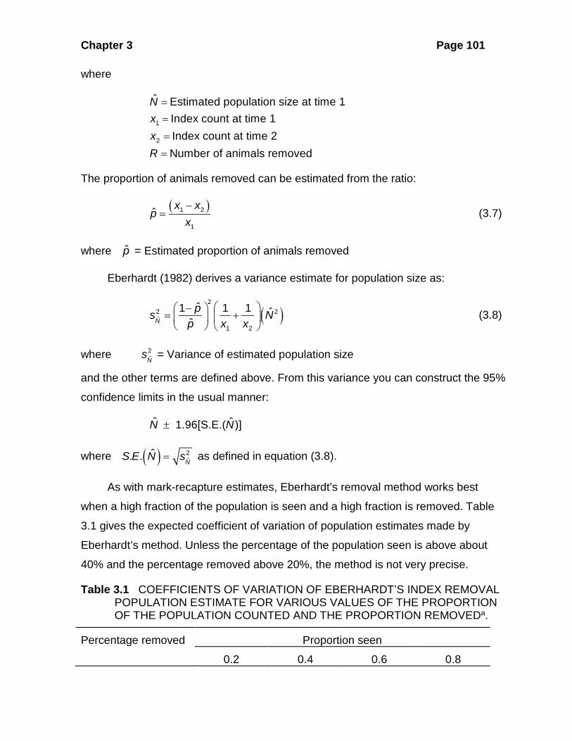
3.1.3 Eberhardt’s Removal Method
A simpler use of removal data to estimate population size was suggested by
Eberhardt (1982) and has been called the “index-removal” method. If an index of
population size (like roadside counts) can be made before and after the removal of a
known number of individuals, it is possible to use the indices to estimate absolute
density. This method does not require you to classify individuals into x-types and y-
types as does the change-in-ratio method, and there is no need to identify
individuals. Eberhardt (1982) discusses how this removal method compares with
methods based on mark-recapture.
To use Eberhardt’s method, an index of population size is measured before and
after the removals. This index is assumed to have some constant but unknown
relationship to population size. For example, a roadside count may see 15% of the
deer in an area. If you know the number of animals removed from the population after
the first index is taken, you can calculate an estimate of population size by the
equation:
1
1 2
ˆ x RNx x
=−
(3.6)
Chapter 3 Page 101
where
1
2
ˆ Estimated population size at time 1Index count at time 1Index count at time 2Number of animals removed
NxxR
==
=
=
The proportion of animals removed can be estimated from the ratio:
( )1 2
1
ˆ x xp
x−
= (3.7)
where p = Estimated proportion of animals removed
Eberhardt (1982) derives a variance estimate for population size as:
( )2
2 2ˆ
1 2
ˆ1 1 1 ˆˆN
ps Np x x
−= +
(3.8)
where 2N
s = Variance of estimated population size
and the other terms are defined above. From this variance you can construct the 95%
confidence limits in the usual manner:
ˆ ˆ 1.96[S.E.( )]N N±
where ( ) 2ˆ
ˆ. .N
S E N s= as defined in equation (3.8).
As with mark-recapture estimates, Eberhardt’s removal method works best
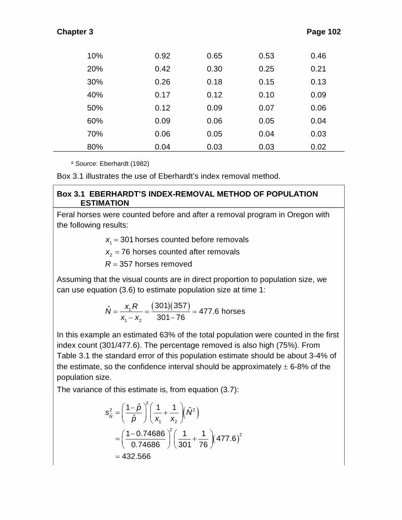
when a high fraction of the population is seen and a high fraction is removed. Table
3.1 gives the expected coefficient of variation of population estimates made by
Eberhardt’s method. Unless the percentage of the population seen is above about
40% and the percentage removed above 20%, the method is not very precise.
Table 3.1 COEFFICIENTS OF VARIATION OF EBERHARDT’S INDEX REMOVAL POPULATION ESTIMATE FOR VARIOUS VALUES OF THE PROPORTION OF THE POPULATION COUNTED AND THE PROPORTION REMOVEDa.
Percentage removed Proportion seen
0.2 0.4 0.6 0.8
Chapter 3 Page 102
10% 0.92 0.65 0.53 0.46 20% 0.42 0.30 0.25 0.21 30% 0.26 0.18 0.15 0.13 40% 0.17 0.12 0.10 0.09 50% 0.12 0.09 0.07 0.06 60% 0.09 0.06 0.05 0.04 70% 0.06 0.05 0.04 0.03 80% 0.04 0.03 0.03 0.02
a Source: Eberhardt (1982)
Box 3.1 illustrates the use of Eberhardt’s index removal method.
Box 3.1 EBERHARDT’S INDEX-REMOVAL METHOD OF POPULATION ESTIMATION
Feral horses were counted before and after a removal program in Oregon with the following results:
1
2
301 horses counted before removals76 horses counted after removals357 horses removed
xxR
=
=
=
Assuming that the visual counts are in direct proportion to population size, we can use equation (3.6) to estimate population size at time 1:
( )( )1
1 2
301 357ˆ 477.6 horses301 76
x RNx x
= = =− −
In this example an estimated 63% of the total population were counted in the first index count (301/477.6). The percentage removed is also high (75%). From Table 3.1 the standard error of this population estimate should be about 3-4% of the estimate, so the confidence interval should be approximately ± 6-8% of the population size. The variance of this estimate is, from equation (3.7):
( )
( )
22 2ˆ
1 2
22
ˆ1 1 1 ˆˆ
1 0.74686 1 1 477.60.74686 301 76
432.566
N
ps Np x x
−= +
− = +
=

Chapter 3 Page 103
From this variance we obtain the 95% confidence limits as:
ˆ ˆ 1.96[S.E.( )]
477.6 1.96 432.566
or 437 to 518
N N±
±
These confidence limits are ± 8.5% of population size. Eberhardt’s removal method is most useful in management situations in which a controlled removal of animals is undertaken and it is not feasible or economic to mark individuals. It must be feasible to count a significant fraction of the whole population to obtain results that have adequate precision.
3.1.4 Catch-Effort Methods
In exploited populations it may be possible to estimate population size by the decline
in catch-per-unit-effort with time. This possibility was first recognized by Leslie and
Davis (1939) who used it to estimate the size of a rat population that was being
exterminated by trapping. DeLury (1947) and Ricker (1975) discuss the method in
more detail. This method is highly restricted in its use because it will work only if a
large enough fraction of the population is removed so that there is a decline in the
catch per unit effort. It will not work if the population is large relative to the removals.
The following assumptions are also critical for this method:
1. The population is closed 2. Probability of each individual being caught in a trap is constant throughout the
experiment 3. All individuals have the same probability of being caught in sample i
The data required for catch-effort models are as follows:
ic = Catch or number of individuals removed at sample time i
iK = Accumulated catch from the start up to the beginning of sample time i
if = Amount of trapping effort expended in sample time i
iF = accumulated amount of trapping effort from the start up to the
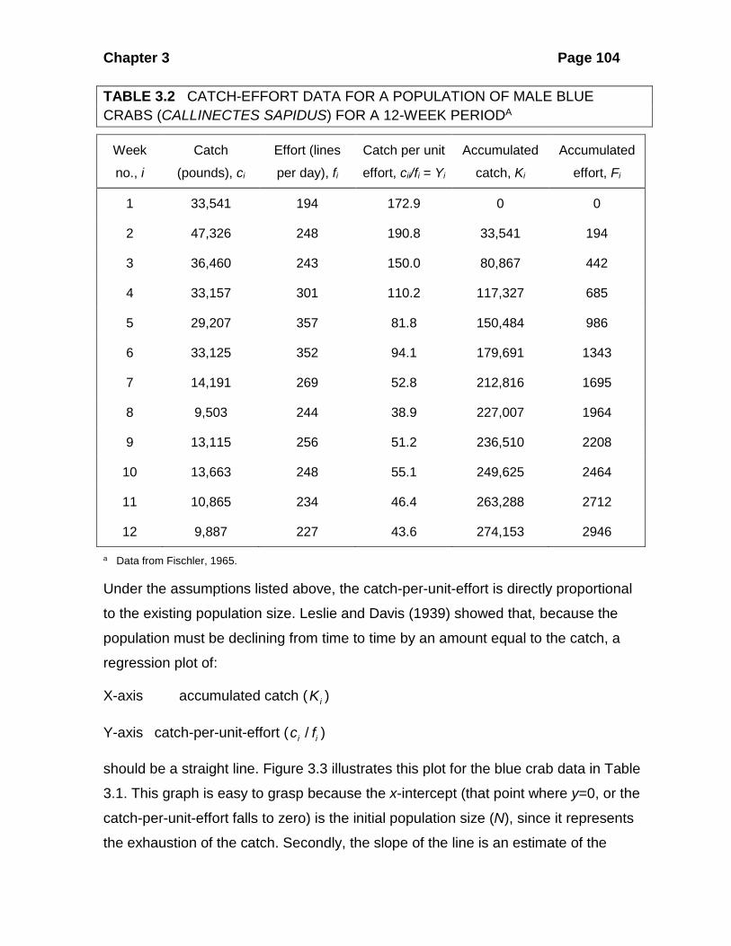
Table 3.2 gives an example of these type of data for a fishery operating on blue
crabs.
Chapter 3 Page 104
TABLE 3.2 CATCH-EFFORT DATA FOR A POPULATION OF MALE BLUE CRABS (CALLINECTES SAPIDUS) FOR A 12-WEEK PERIODA
Week
no., i
Catch
(pounds), ci
Effort (lines
per day), fi
Catch per unit
effort, cii/fi = Yi
Accumulated
catch, Ki
Accumulated
effort, Fi
1 33,541 194 172.9 0 0
2 47,326 248 190.8 33,541 194
3 36,460 243 150.0 80,867 442
4 33,157 301 110.2 117,327 685
5 29,207 357 81.8 150,484 986
6 33,125 352 94.1 179,691 1343
7 14,191 269 52.8 212,816 1695
8 9,503 244 38.9 227,007 1964
9 13,115 256 51.2 236,510 2208
10 13,663 248 55.1 249,625 2464
11 10,865 234 46.4 263,288 2712
12 9,887 227 43.6 274,153 2946
a Data from Fischler, 1965.
Under the assumptions listed above, the catch-per-unit-effort is directly proportional
to the existing population size. Leslie and Davis (1939) showed that, because the
population must be declining from time to time by an amount equal to the catch, a
regression plot of:
X-axis accumulated catch ( iK )
Y-axis catch-per-unit-effort ( /i ic f )
should be a straight line. Figure 3.3 illustrates this plot for the blue crab data in Table
3.1. This graph is easy to grasp because the x-intercept (that point where y=0, or the
catch-per-unit-effort falls to zero) is the initial population size (N), since it represents
the exhaustion of the catch. Secondly, the slope of the line is an estimate of the
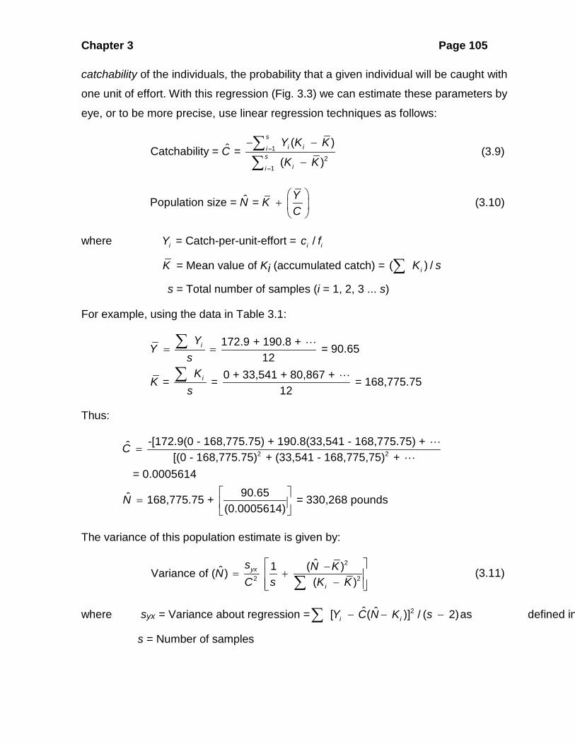
Chapter 3 Page 105
catchability of the individuals, the probability that a given individual will be caught with
one unit of effort. With this regression (Fig. 3.3) we can estimate these parameters by
eye, or to be more precise, use linear regression techniques as follows:
12
1
( )ˆCatchability = = ( )
si ii
sii
Y K KC
K K=
=
− −
−∑∑
(3.9)
ˆPopulation size = = YN KC
+
(3.10)
where iY = Catch-per-unit-effort = /i ic f
K = Mean value of Ki (accumulated catch) = ( ) /iK s∑
s = Total number of samples (i = 1, 2, 3 ... s)
For example, using the data in Table 3.1:
172.9 + 190.8 + = 90.6512
0 + 33,541 + 80,867 + = = = 168,775.7512
i
i
YY
sK
Ks
= =∑
∑
Thus:
2 2-[172.9(0 - 168,775.75) + 190.8(33,541 - 168,775.75) + ˆ
[(0 - 168,775.75) + (33,541 - 168,775,75) + = 0.0005614
90.65ˆ 168,775.75 + = 330,268 pounds(0.0005614)
C
N
=
=
The variance of this population estimate is given by:
2
2 2
ˆ1 ( )ˆVariance of ( )( )
yx
i
s N KNC s K K
−= +
− ∑ (3.11)
where syx = Variance about regression = 2ˆ ˆ[ ( )] / ( 2)i iY C N K s− − −∑ as defined in
s = Number of samples
Chapter 3 Page 106
When the number of samples is large (s > 10), approximate 95% confidence limits
are obtained in the usual way:
ˆ ˆStandard error of = Variance of ˆ ˆ95% confidence limits = 1.96[S.E.( )]
N N
N N±
When the number of samples is small, use the general method outlined in Seber
(1982, pg. 299) to get confidence limits on N .
The plot shown in Figure 3.3 provides a rough visual check on the assumptions
of this model. If the data do not seem to fit a straight line, or if the variance about the
regression line is not constant, the data violate some or all of the assumptions and
this model is not appropriate. Ricker (1975) discusses how to deal with certain cases
in which the assumptions of the model are not fulfilled.
Figure 3.3 Leslie plot of catch-effort data of Fischler (1965) for a population of male blue crabs. Using the Leslie model, one can estimate initial population size (N) by extrapolating
the linear regression to the X-axis. In this case (arrow) N is about 330 x 103 pounds. (Original data in Table 3.1.)
Accumulated catch, Ki (thousands of pounds)0 50 100 150 200 250 300 350
Cat
ch p
er u
nit e
ffort
, Yi
0
50
100
150
200
Chapter 3 Page 107
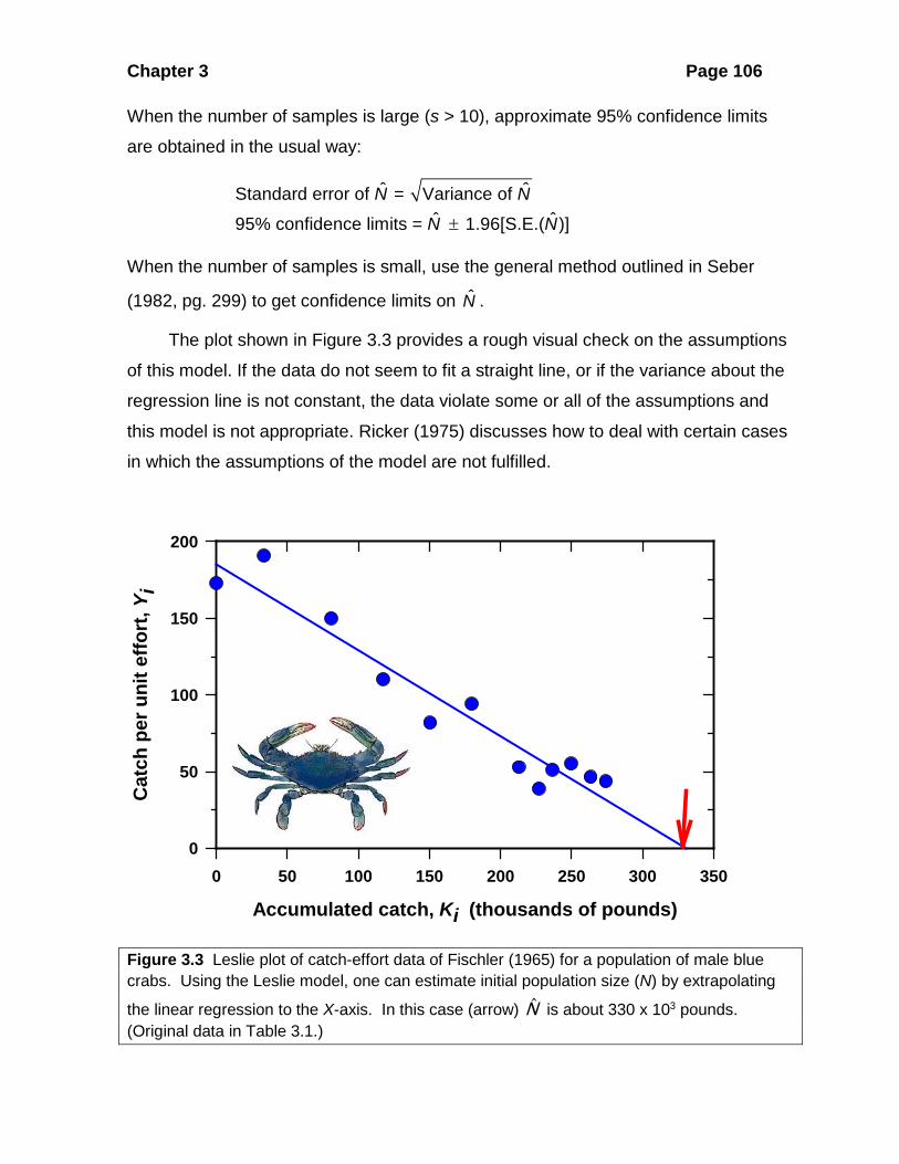
DeLury (1947) and Ricker (1975) provide two alternative models for analyzing
catch-effort data based on a semi-logarithmic relationship between the log of the
catch-per-unit-effort (y-axis) and the accumulated fishing effort ( iF ) on the x-axis (e.g.
Fig. 3.4). The calculations are again based on linear regression techniques. For the
more general Ricker model: defining iz = log( iY ) we have -
12
1
( )ˆlog(1- )( )
si ii
sii
z F FC
F F=
=
−=
−∑∑
(3.12)
and
ˆ ˆˆlog log(1- ) log N z F C C= − − (3.13)
and parameter estimates of catchability (C ) and population size ( N ) are obtained by
taking antilogs. Seber (1982, p. 302) and Ricker (1975) show how confidence
intervals may be calculated for these semi-logarithmic models.
Since the Leslie model (eq. 3.10) and the Ricker model (eq. 3.13) are based on
somewhat alternative approaches, it is desirable to plot both the Leslie regression
(e.g. Fig. 3.3) and the Ricker semi-log regression (Fig. 3.4) as checks on whether the
underlying assumptions may be violated.
Chapter 3 Page 108
Figure 3.4 Ricker plot of catch-effort data of Fischler (1965) for male blue crabs. This is a semilogarithmic plot of the data in Table 3.2 in which the y-axis is the log of the catch per unit effort. The graph shows a curved line and not a straight line, and consequently the Ricker catch-effort model is not supported for these data
The program RECAP in Appendix 2 (page 000) can do these calculations for
the catch-effort models of Leslie and Ricker described in this section and calculates
confidence intervals for population size for both estimators.
Population estimation by the removal method is subject to many pitfalls.
Braaten (1969) showed by computer simulation that the DeLury (1947) semi-
logarithmic model produces population estimates that are biased by being too low on
average. This bias can be eliminated by regressing the log of the catch-per-unit-effort
against the accumulated fishing effort ( iF ) plus half the effort expended in the i-
interval ( 12 if ) (Braaten 1969). The more serious problem of variable catchability has
been discussed by Schnute (1983) who proposes a new method of population
estimation for the removal method based on maximum-likelihood models. In
particular, Schnute (1983) provides a method of testing for constant catchability and
Accumulated effort, Fi
0 500 1000 1500 2000 2500 3000
Log
of c
atch
per
uni
t effo
rt
1.5
1.6
1.7
1.8
1.9
2.0
2.1
2.2
2.3
Chapter 3 Page 109
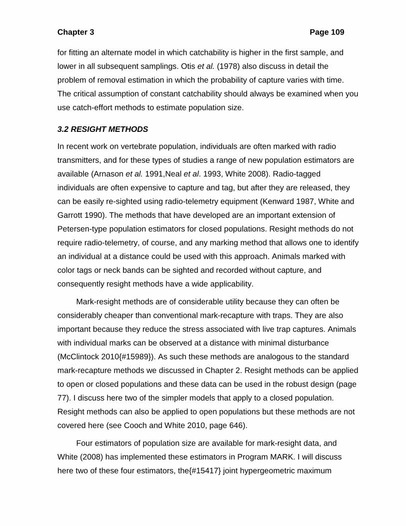
for fitting an alternate model in which catchability is higher in the first sample, and
lower in all subsequent samplings. Otis et al. (1978) also discuss in detail the
problem of removal estimation in which the probability of capture varies with time.
The critical assumption of constant catchability should always be examined when you
use catch-effort methods to estimate population size.
3.2 RESIGHT METHODS
In recent work on vertebrate population, individuals are often marked with radio
transmitters, and for these types of studies a range of new population estimators are
available (Arnason et al. 1991,Neal et al. 1993, White 2008). Radio-tagged
individuals are often expensive to capture and tag, but after they are released, they
can be easily re-sighted using radio-telemetry equipment (Kenward 1987, White and
Garrott 1990). The methods that have developed are an important extension of
Petersen-type population estimators for closed populations. Resight methods do not
require radio-telemetry, of course, and any marking method that allows one to identify
an individual at a distance could be used with this approach. Animals marked with
color tags or neck bands can be sighted and recorded without capture, and
consequently resight methods have a wide applicability.
Mark-resight methods are of considerable utility because they can often be
considerably cheaper than conventional mark-recapture with traps. They are also
important because they reduce the stress associated with live trap captures. Animals
with individual marks can be observed at a distance with minimal disturbance
(McClintock 2010{#15989}). As such these methods are analogous to the standard
mark-recapture methods we discussed in Chapter 2. Resight methods can be applied
to open or closed populations and these data can be used in the robust design (page
77). I discuss here two of the simpler models that apply to a closed population.
Resight methods can also be applied to open populations but these methods are not
covered here (see Cooch and White 2010, page 646).
Four estimators of population size are available for mark-resight data, and
White (2008) has implemented these estimators in Program MARK. I will discuss
here two of these four estimators, the{#15417} joint hypergeometric maximum
Chapter 3 Page 110
likelihood estimator (JHE) and Bowden’s estimator. The statistical theory behind the
JHE estimator is beyond the scope of this book, and is discussed in detail in Cooch
and White (2010). I would like to provide a general understanding of how maximum
likelihood estimators are derived since they form the core of much of modern
estimation theory for mark-recapture estimates.
Maximum likelihood is a method of statistical inference in which a particular
model is evaluated with reference to a set of data. In this case we have a set of
observations based on the sighting frequencies of marked and unmarked animals. If
we assume that re-sightings occur at random, we can connect through probability
theory the observed data and the likely value of population size N. For simple
situations, such as the Petersen method, in which only two sampling times are
involved the resulting estimator for N will be a simple equation like equation (2.2). For
more complex situations, involving several sampling times, the resulting estimator
cannot be written as a simple equation with a solution and one must search to find
the best value of N by trial and error. In mathematical jargon one searches for the
maximum value of a function called the likelihood function (Edwards 1972{ #4877}).
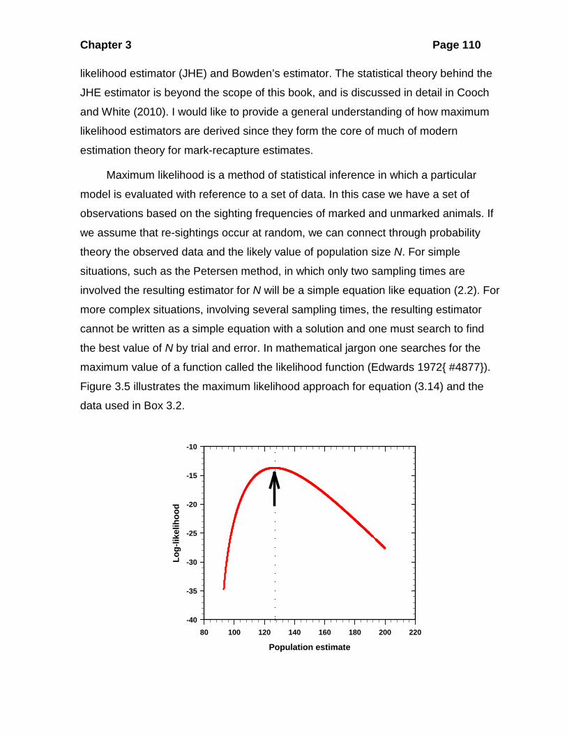
Figure 3.5 illustrates the maximum likelihood approach for equation (3.14) and the
data used in Box 3.2.
Population estimate80 100 120 140 160 180 200 220
Log-
likel
ihoo
d
-40
-35
-30
-25
-20
-15
-10
Chapter 3 Page 111
Figure 3.5 Likelihood ratio for the mountain sheep example given in Box 3.2. Given the observed data, estimated population sizes are substituted in equation (3.10) and the likelihood calculated. The most probable value of N is that which gives the highest likelihood
(arrow), in this case N = 127 (dashed line and arrow) at which point the log likelihood is -13.6746 (likelihood = 1.1513 x 10⁻⁶). Because likelihoods cover a broad numerical range it is easier to graph them as log-likelihoods (loge or ln) as we have done here.
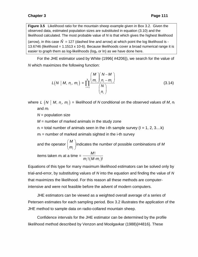
For the JHE estimator used by White (1996{ #4206}), we search for the value of
N which maximizes the following function:
( )k
i = 1 , , = i i i
i i
i
M N Mm n m
L N M n mNn
− −
∏ (3.14)
where ( ) , , =i iL N M n m likelihood of N conditional on the observed values of M, ni and mi
N = population size M = number of marked animals in the study zone ni = total number of animals seen in the i-th sample survey (I = 1, 2, 3....k) mi = number of marked animals sighted in the i-th survey
and the operator i
Mm
indicates the number of possible combinations of M
items taken mi at a time = ( )
!! - !i i
Mm M m
Equations of this type for many maximum likelihood estimators can be solved only by
trial-and-error, by substituting values of N into the equation and finding the value of N
that maximizes the likelihood. For this reason all these methods are computer-
intensive and were not feasible before the advent of modern computers.
JHE estimators can be viewed as a weighted overall average of a series of
Petersen estimates for each sampling period. Box 3.2 illustrates the application of the
JHE method to sample data on radio-collared mountain sheep.
Confidence intervals for the JHE estimator can be determined by the profile
likelihood method described by Venzon and Moolgavkar (1988){#4816}. These
Chapter 3 Page 112
methods are computer intensive and will not be described here. They are available in
Program MARK.
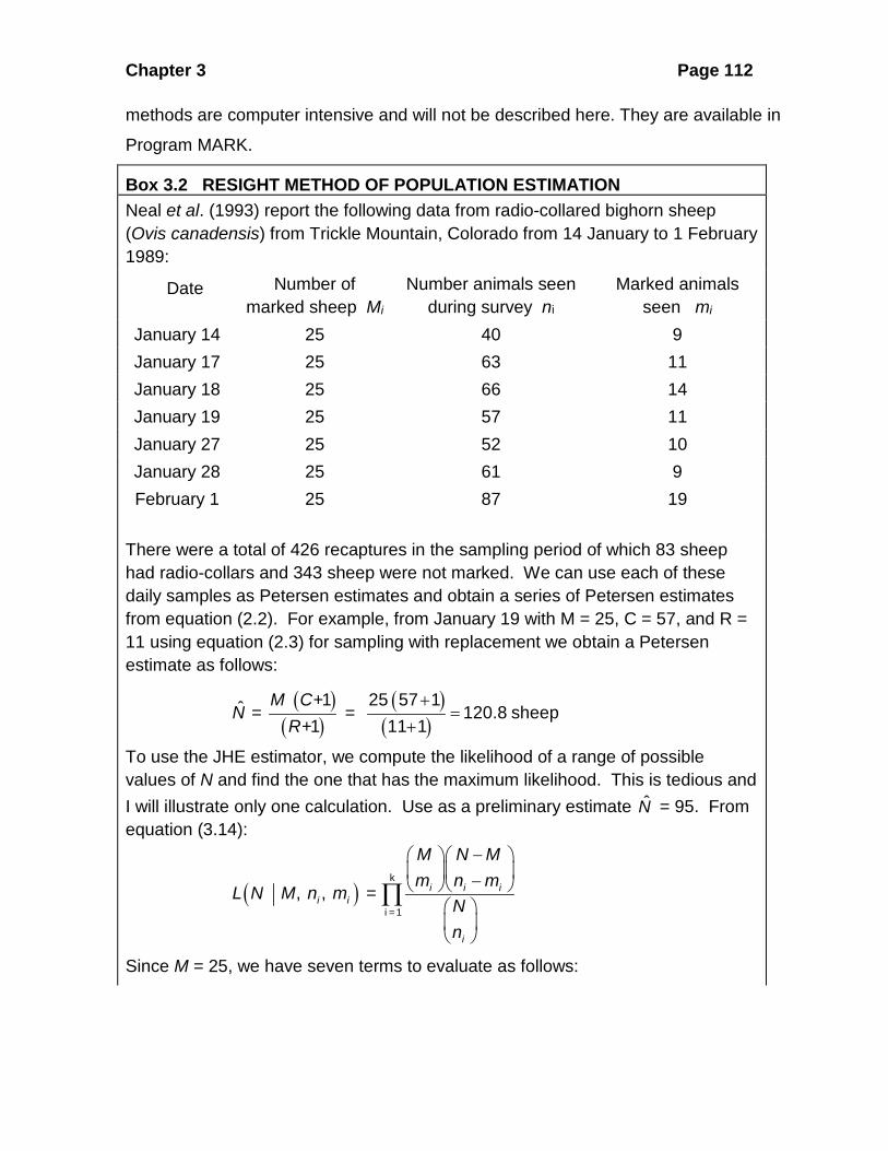
Box 3.2 RESIGHT METHOD OF POPULATION ESTIMATION Neal et al. (1993) report the following data from radio-collared bighorn sheep (Ovis canadensis) from Trickle Mountain, Colorado from 14 January to 1 February 1989:
Date Number of marked sheep Mi
Number animals seen during survey ni
Marked animals seen mi
January 14 25 40 9 January 17 25 63 11 January 18 25 66 14 January 19 25 57 11 January 27 25 52 10 January 28 25 61 9 February 1
25 87 19
There were a total of 426 recaptures in the sampling period of which 83 sheep had radio-collars and 343 sheep were not marked. We can use each of these daily samples as Petersen estimates and obtain a series of Petersen estimates from equation (2.2). For example, from January 19 with M = 25, C = 57, and R = 11 using equation (2.3) for sampling with replacement we obtain a Petersen estimate as follows:
( )( ) +1ˆ =
+1M C
NR
= ( )( )
25 57 1120.8 sheep
11 1+
=+
To use the JHE estimator, we compute the likelihood of a range of possible values of N and find the one that has the maximum likelihood. This is tedious and I will illustrate only one calculation. Use as a preliminary estimate N = 95. From equation (3.14):
( )k
i = 1 , , = i i i
i i
i
M N Mm n m
L N M n mNn
− −
∏
Since M = 25, we have seven terms to evaluate as follows:
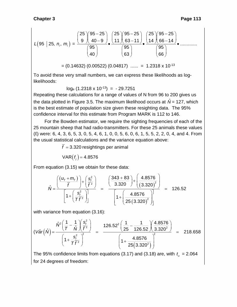
Chapter 3 Page 113
( )25 95 25 25 95 25 25 95 259 40 9 11 63 11 14 66 1495 25, , = .............
95 95 9540 63 66
i iL n m
− − − − − − • • •
= (0.14632) (0.00522) (0.04817) ...... = 1.2318 x 10⁻¹³
To avoid these very small numbers, we can express these likelihoods as log-likelihoods: loge (1.2318 x 10⁻¹³) = - 29.7251 Repeating these calculations for a range of values of N from 96 to 200 gives us the data plotted in Figure 3.5. The maximum likelihood occurs at N = 127, which is the best estimate of population size given these resighting data. The 95% confidence interval for this estimate from Program MARK is 112 to 146. For the Bowden estimator, we require the sighting frequencies of each of the 25 mountain sheep that had radio-transmitters. For these 25 animals these values (fi) were: 6, 4, 3, 6, 5, 3, 0, 5, 4, 6, 1, 0, 0, 5, 6, 0, 6, 1, 5, 5, 2, 2, 0, 4, and 4. From the usual statistical calculations and the variance equation above: 3.320 resightings per animalf =
( )VAR 4.8576jf =
From equation (3.15) we obtain for these data:
( )( )
( )
2
22
2
2 2
343 83 4.85763.320 3.320ˆ 126.52
4.85761 125 3.320
T T f
f
u m sf f
Ns
T f
+ + ++ = = =
+ +
with variance from equation (3.16):
( ( )
( )
22 2
2 2
2 22
2 2
1 1 1 1 4.8576ˆ 126.52ˆ 25 126.52 3.320ˆˆ 218.6584.85761 1
25 3.320
f
f
sNT fNVar N
sT f
− − = = =
+ +
The 95% confidence limits from equations (3.17) and (3.18) are, with tα = 2.064 for 24 degrees of freedom:

Chapter 3 Page 114
( )( ) 218.6582.064 126.52
ˆ 126.52Lower confidence limit = 99ˆexp CV e
Nt Nα
= =
( ) ( )( )( ) ( )218.6582.064 126.52ˆ ˆ ˆUpper confidence limit of exp t CV 126.52 e
161
N N Nα
= =
=Note that these confidence limits are slightly wider than those given for the JHE estimator above. This is the price one pays for the less restrictive assumption that individual sheep may have different probabilities of being sighted on the study area. These calculations are done by Program RECAP (page 000) and by Program MARK from White (2008).
The JHE method assumes that all the marked animals remain on the study area
during the surveys. Thus the number of marked animals is constant, and the
probability of re-sighting must be constant from sample to sample to obtain a valid
closed population estimate. Day to day variation in sightability can not be
accommodated in this model but can be allowed in the next model (McClintock
2010).
Bowden (1995) developed an estimate for population size with mark-resight
data that allows us to relax the assumption that all individuals in the population have
the same probability of resighting. To compute this estimator, we need to have the
resighting frequency for each individually-tagged individual in the population. Some
animals may not be seen at all, and some may be seen at every one of the sampling
times. The Bowden estimator of population size is given by:
( ) 2
2
2
2
ˆ
1
T T f
f
u m sf f
Ns
T f
+ +
=
+
(3.15)
where uT = total number of sightings of unmarked animals over all periods
mT = total number of sightings of marked animals over all time periods
f = mean resighting frequency of marked animals = mT / T
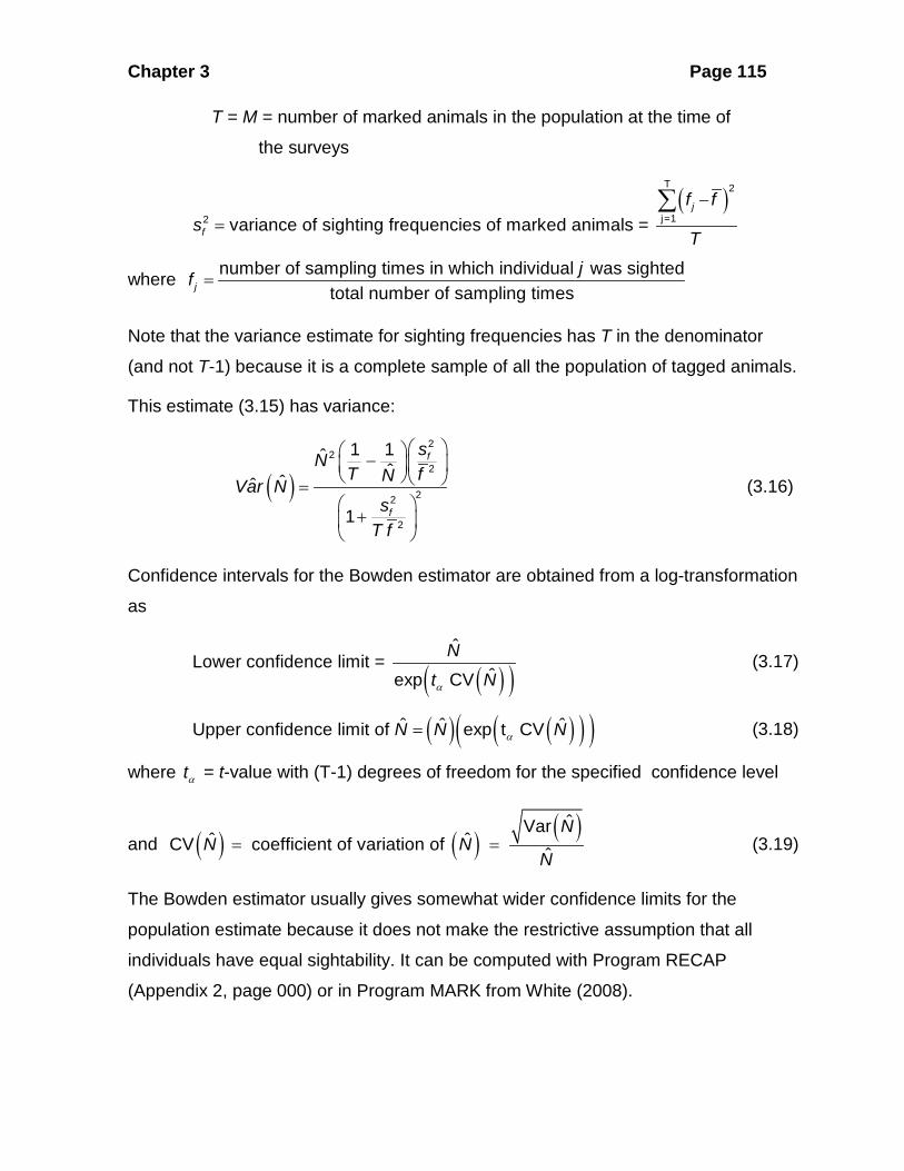
Chapter 3 Page 115
T = M = number of marked animals in the population at the time of
the surveys
( )T 2
j=12 variance of sighting frequencies of marked animals = j
f
f fs
T
−=
∑
where number of sampling times in which individual was sightedtotal number of sampling timesj
jf =
Note that the variance estimate for sighting frequencies has T in the denominator
(and not T-1) because it is a complete sample of all the population of tagged animals.
This estimate (3.15) has variance:
( )2
22
22
2
1 1ˆˆˆˆ
1
f
f
sNT fNVar N
sT f
− =
+
(3.16)
Confidence intervals for the Bowden estimator are obtained from a log-transformation
as
( )( )ˆ
Lower confidence limit = ˆexp CV
Nt Nα
(3.17)
( ) ( )( )( )ˆ ˆ ˆUpper confidence limit of exp t CVN N Nα= (3.18)
where tα = t-value with (T-1) degrees of freedom for the specified confidence level
and ( ) ( ) ( )ˆVarˆ ˆCV coefficient of variation of ˆ
NN N
N= = (3.19)
The Bowden estimator usually gives somewhat wider confidence limits for the
population estimate because it does not make the restrictive assumption that all
individuals have equal sightability. It can be computed with Program RECAP
(Appendix 2, page 000) or in Program MARK from White (2008).
Chapter 3 Page 116
Resight methods can be also developed for open populations by the use of the
robust design (Figure 2.7, page 77). McClintock (2010) describes the details of how
to carry out this approach using Program MARK. In addition if the marked animals
have radio-collars, it may be possible to determine which individuals are outside of
the study area either permanently or temporarily. These data would allow emigration
and immigration estimates to be determined. Details are given in McClintock (2010).
The movements of radio-collared animals are not relevant for obtaining estimates of
abundance but are critical for estimates of density, as we will discuss below.
The technological innovation of adding a GPS (global positioning system) to
radio collars has greatly enhanced the ability of ecologists to get frequent movement
data on wide-ranging animals. For density estimates these movement data are of
limited use, but they can greatly assist in the estimation of survival rates and
reproductive rates (Conroy et al. 2000{#7531}), as well as habitat selection for large
carnivores and other threatened species (Hebblewhite and Haydon 2010{ #15811}).
As always in ecological studies we should be clear about the question being asked
and not have technology rule what we study.
3.3 ENUMERATION METHODS Why estimate when you can count the entire population? This is one possible
response to the problems of estimating density by mark-recapture, removal, or
resight methods. All of these methods have their assumptions, and you could avoid
all this statistical hassle by counting all the organisms in the population. In most
cases this simple solution is not possible either physically or financially, and one must
rely on a sampling method of some type. But there are a few situations in which
enumeration is a possible strategy.
Enumeration methods have been used widely in small mammal studies (Krebs
1966) where they have been called the minimum-number-alive method (MNA). The
principle of this method is simple. Consider a small example from a mark-recapture
study (0 = not caught, 1 = caught):
Tag no. Time 1 Time 2 Time 3 Time 4 Time 5 A34 1 0 1 1 0
Chapter 3 Page 117
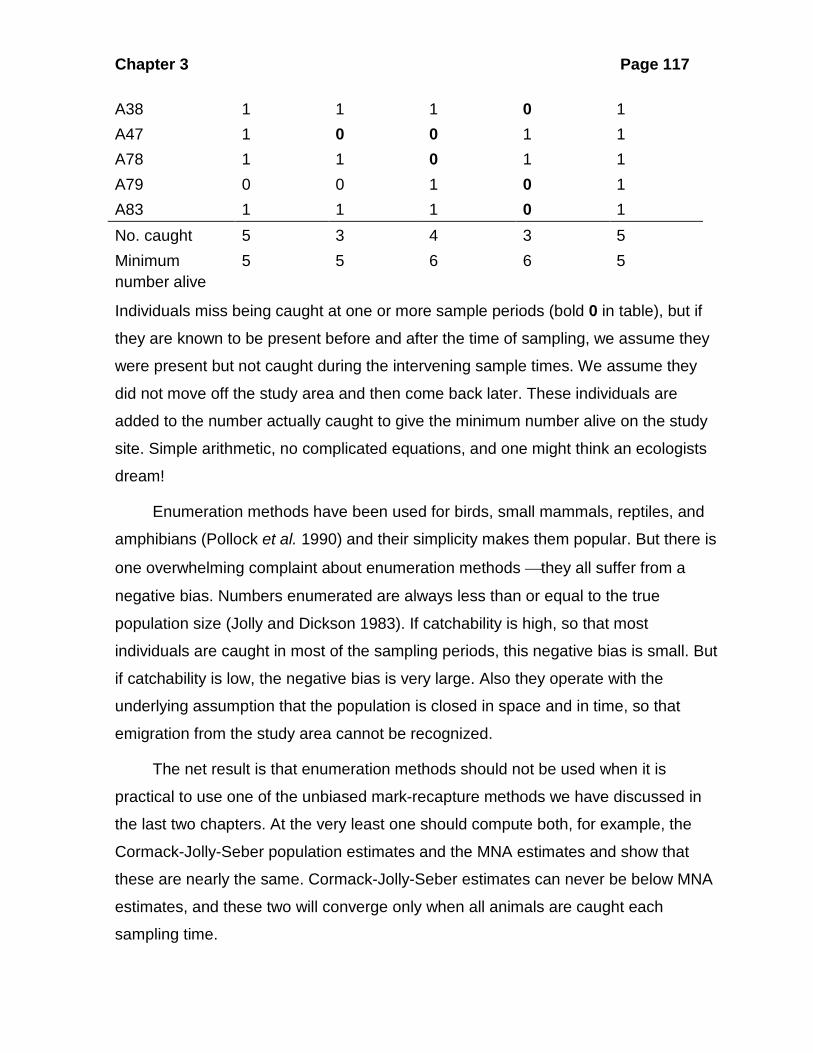
A38 1 1 1 0 1 A47 1 0 0 1 1 A78 1 1 0 1 1 A79 0 0 1 0 1 A83 1 1 1 0 1 No. caught 5 3 4 3 5 Minimum number alive
5 5 6 6 5
Individuals miss being caught at one or more sample periods (bold 0 in table), but if
they are known to be present before and after the time of sampling, we assume they
were present but not caught during the intervening sample times. We assume they
did not move off the study area and then come back later. These individuals are
added to the number actually caught to give the minimum number alive on the study
site. Simple arithmetic, no complicated equations, and one might think an ecologists
dream!
Enumeration methods have been used for birds, small mammals, reptiles, and
amphibians (Pollock et al. 1990) and their simplicity makes them popular. But there is
one overwhelming complaint about enumeration methods they all suffer from a
negative bias. Numbers enumerated are always less than or equal to the true
population size (Jolly and Dickson 1983). If catchability is high, so that most
individuals are caught in most of the sampling periods, this negative bias is small. But
if catchability is low, the negative bias is very large. Also they operate with the
underlying assumption that the population is closed in space and in time, so that
emigration from the study area cannot be recognized.
The net result is that enumeration methods should not be used when it is
practical to use one of the unbiased mark-recapture methods we have discussed in
the last two chapters. At the very least one should compute both, for example, the
Cormack-Jolly-Seber population estimates and the MNA estimates and show that
these are nearly the same. Cormack-Jolly-Seber estimates can never be below MNA
estimates, and these two will converge only when all animals are caught each
sampling time.
Chapter 3 Page 118
In a few cases enumeration methods are needed and can be justified on the
principle that a negatively biased estimate of population size is better than no
estimate. In some cases the numbers of animals in the population are so low that
recaptures are rare. In other cases with endangered species it may not be possible to
mark and recapture animals continuously without possible damage so sample sizes
may be less than the 5-10 individuals needed for most estimators to be unbiased. In
these cases it is necessary to ask whether a population estimate is needed, or
whether an index of abundance is sufficient for management purposes. It may also
be possible to use the methods presented in the nest two chapters for rare and
endangered species. The important point is to recognize that complete enumeration
is rarely a satisfactory method for estimating population size.
The fact that most animals do not satisfy the randomness-of-capture
assumption of mark-recapture models is often used to justify the use of enumeration
as an alternative estimation procedure. But Pollock et al. (1990) show that even with
heterogeneity of capture the Cormack-Jolly-Seber model is less biased than MNA
based enumeration procedures. A closed population estimator or the Cormack-Jolly-
Seber model should be used in almost all cases instead of enumeration.
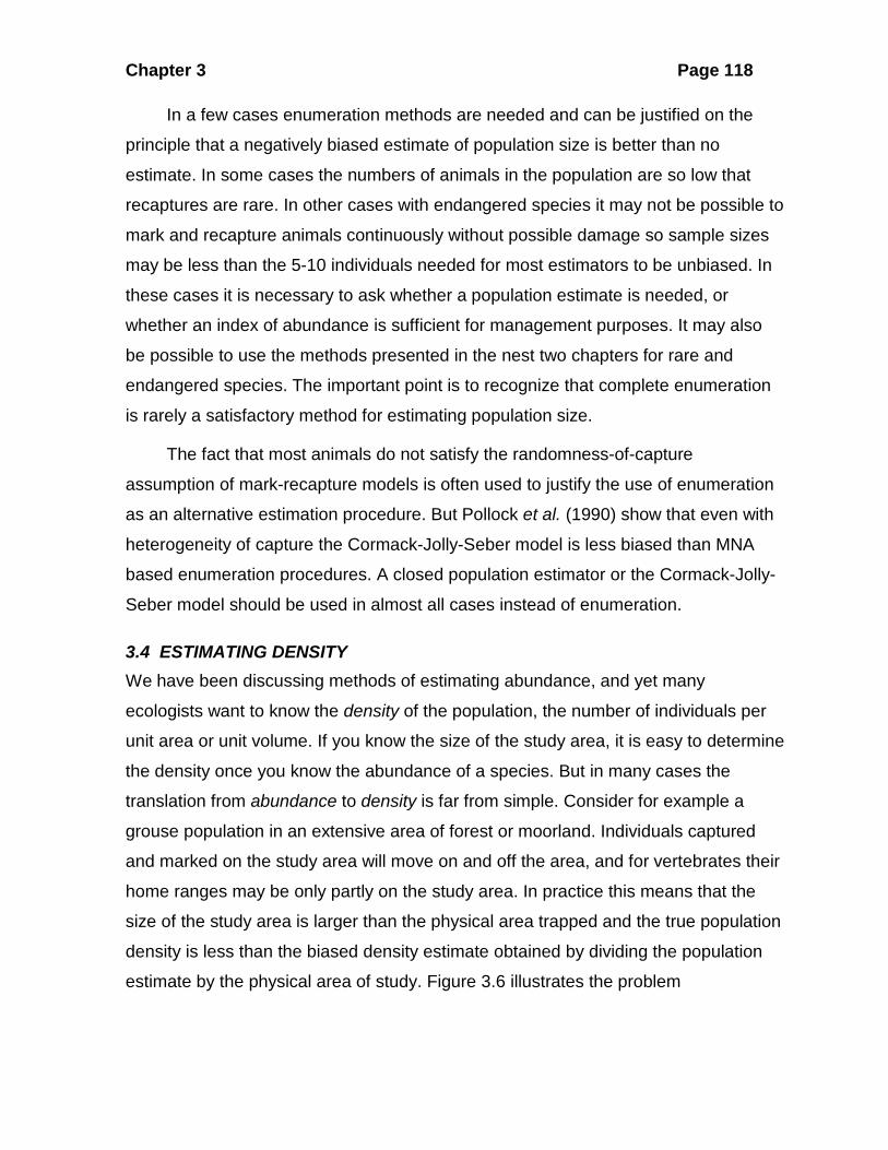
3.4 ESTIMATING DENSITY We have been discussing methods of estimating abundance, and yet many
ecologists want to know the density of the population, the number of individuals per
unit area or unit volume. If you know the size of the study area, it is easy to determine
the density once you know the abundance of a species. But in many cases the
translation from abundance to density is far from simple. Consider for example a
grouse population in an extensive area of forest or moorland. Individuals captured
and marked on the study area will move on and off the area, and for vertebrates their
home ranges may be only partly on the study area. In practice this means that the
size of the study area is larger than the physical area trapped and the true population
density is less than the biased density estimate obtained by dividing the population
estimate by the physical area of study. Figure 3.6 illustrates the problem
Chapter 3 Page 119
schematically. How can we determine how large an effective area we are studying so
that we can obtain estimates of true density?
Several methods have been employed to estimate the effective size of a
trapping area.
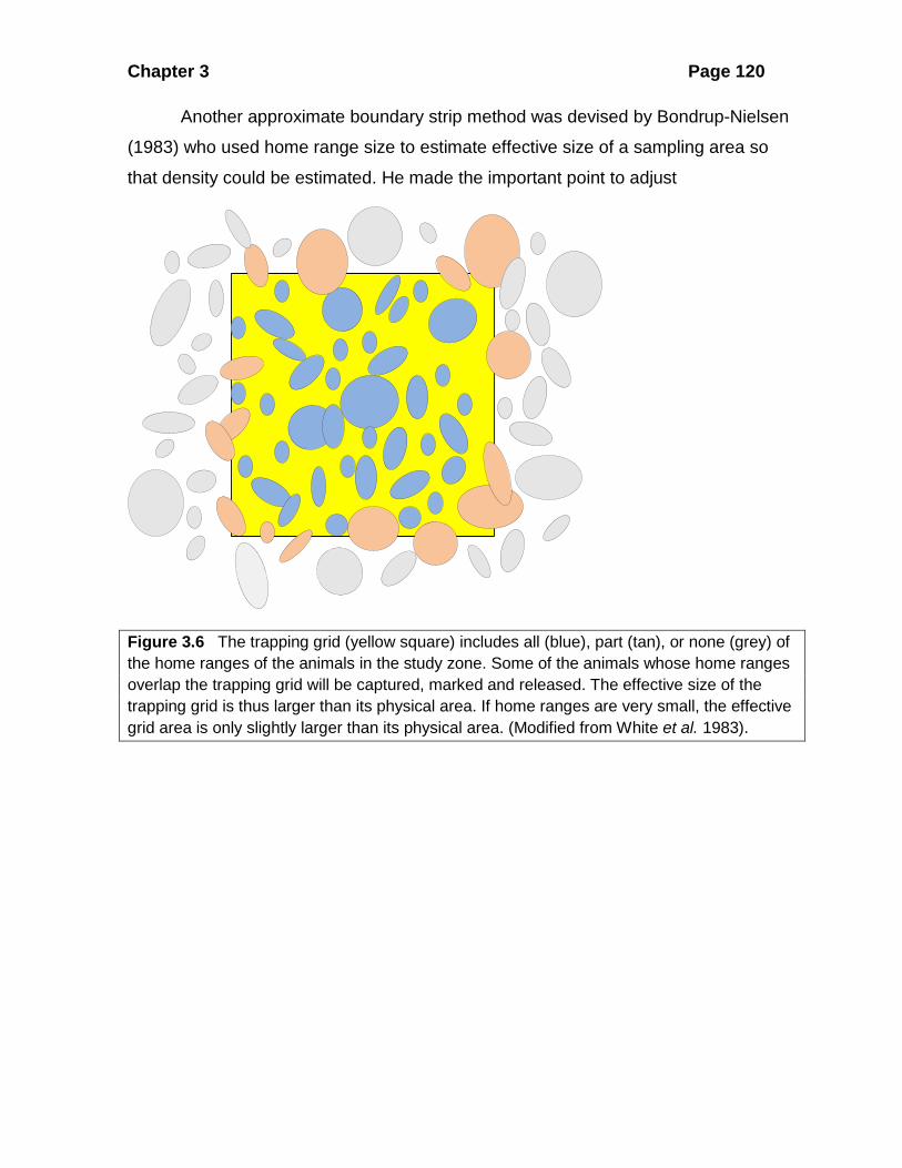
3.4.1 Boundary Strip Methods
The simplest methods add a boundary strip around the trapping area to estimate the
effective size of area trapped. Figure 3.7 illustrates the principle of a boundary strip.
The width of the boundary strip can be estimated in several ways (Stenseth and
Hansson 1979). The simplest procedure is to add a strip one-half the movement
radius of the animals under study. For example, in mammals one can determine the
average distance moved between trap captures and use this as a likely estimate of
movement radius. The problem with this approach is that it is highly dependent on
the spacing between the capture points, and the number of recaptures. While this
approach is better than ignoring the problem of a boundary strip, it is not completely
satisfactory (Otis et al. 1978).
Boundary strip width can be estimated in several ways. Two are most common
and both rely on multiple recaptures in order to estimate a correlate of the home
range size of the animals being studied (Wilson and Anderson 1985{#15990}). The
mean-maximum-distance-moved (MMDM) estimator calculates for each individual
the maximum distance between capture points and obtains a mean of these values
(Jett and Nichols 1987{#1903}). This value of MMDM can then be divided by two to
estimate the width of the boundary strip. An alternative that used the same data is to
calculate the asymptotic range length (ARL) from the same data by fitting an
asymptotic regression to the number of captures (X) versus the observed range
length (Y) for each animal. The assumption is that as you obtain more and more
captures on an individual, the home range length will increase up to some maximum,
which is then used as an estimate of boundary strip width. Both MMDM and ARL can
be calculated for a set of closed population data in Program DENSITY described
below.
Chapter 3 Page 120
Another approximate boundary strip method was devised by Bondrup-Nielsen
(1983) who used home range size to estimate effective size of a sampling area so
that density could be estimated. He made the important point to adjust
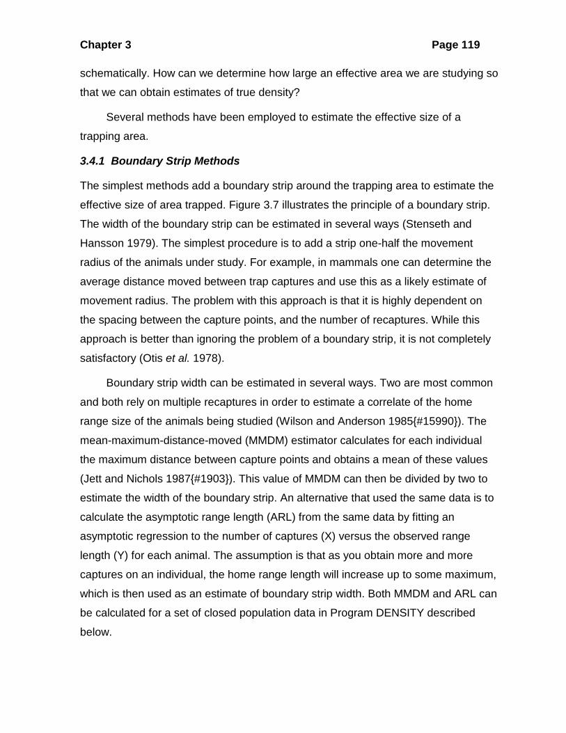
Figure 3.6 The trapping grid (yellow square) includes all (blue), part (tan), or none (grey) of the home ranges of the animals in the study zone. Some of the animals whose home ranges overlap the trapping grid will be captured, marked and released. The effective size of the trapping grid is thus larger than its physical area. If home ranges are very small, the effective grid area is only slightly larger than its physical area. (Modified from White et al. 1983).
Chapter 3 Page 121
Figure 3.7 Illustration of a study grid of 10 x 10 checkerboard shape with a boundary strip added to delineate the effective study area. Population size would be estimated for the checkerboard and the total area including the boundary strip would be used to estimate population density.
sampling grid size to minimize the boundary strip effect by defining the required size
of the sampling area. This method proceeds in three steps:
1. Calculate the average home range size for the animal under study. Methods for doing this are presented in Kenward (1987), White and Garrott (1990), and Seaman et al. (1998), and evaluated by Downs et al. (2012). {#5583} { #16007}
2. Compute the ratio of grid size to area of the average home range. In a hypothetical world with square home ranges that do not overlap, the overestimation of density is shown by Bondrup-Nielsen (1983) to be:
( )21Estimated density
True density
A
A
+= (3.25)
where area of study gridaverage home range size
A = (3.26)
3. Assume that the home range is elliptical and in a computer “throw” home ranges at random on a map that delineates the study zone as part of a large area of habitat.
Trapping grid
Boundary strip

Chapter 3 Page 122
Figure 3.8 shows the results of this simulation. On the basis of this graph,
Bondrup-Nielsen (1983{ #801}) suggested that the trapping grid size should be at
least 16 times the size of the average home range of the species under study to
minimize the edge effect.
Figure 3.8 Expected relationship between relative grid size (grid size / home range size) and the overestimation of density if no boundary strip is used to calculate population density. The theoretical curve is shown for square home ranges that do not overlap, and the red points show the average results of computer simulations with elliptical home ranges that are allowed to overlap. (Modified from Bondrup-Nielsen 1983).
Given that we have data on study area size and average home range size, we
can use Figure 3.8 as a guide to estimating true density of a population. For example,
in a study of house mouse populations in wheat fields live-traps were set out on a 0.8
ha grid, and the Petersen population estimate was 127 mice. The average home
range size of these house mice was 0.34 ha. We can calculate from equation (3.26):
Grid size 0.8 2.35Home range size 0.34
A = = =
From Figure 3.8 or equation (3.25) the expected overestimate is
Grid size / home range size0 5 10 15 20 25
Estim
ated
den
sity
/ tr
ue d
ensi
ty
0
2
4
6
8
10
12
recommended ratioof grid size to home range size
Chapter 3 Page 123
( ) ( )2 21 2.35 1Estimated density 2.73
True density 2.35
A
A
+ += = =
This the biased density estimated from the area of the grid:
Population estimate 127 miceBiased density estimate Size of study area 0.8 ha
159 mice per ha159Corrected density estimate 58 mice per ha2.73
= =
=
= =
This correction factor is only approximate because home ranges are variable in size
and not exactly elliptical and there is some overlap among individuals, but the
adjusted density estimate is closer to the true value than is the biased estimate that
does not take into account the effective grid size.
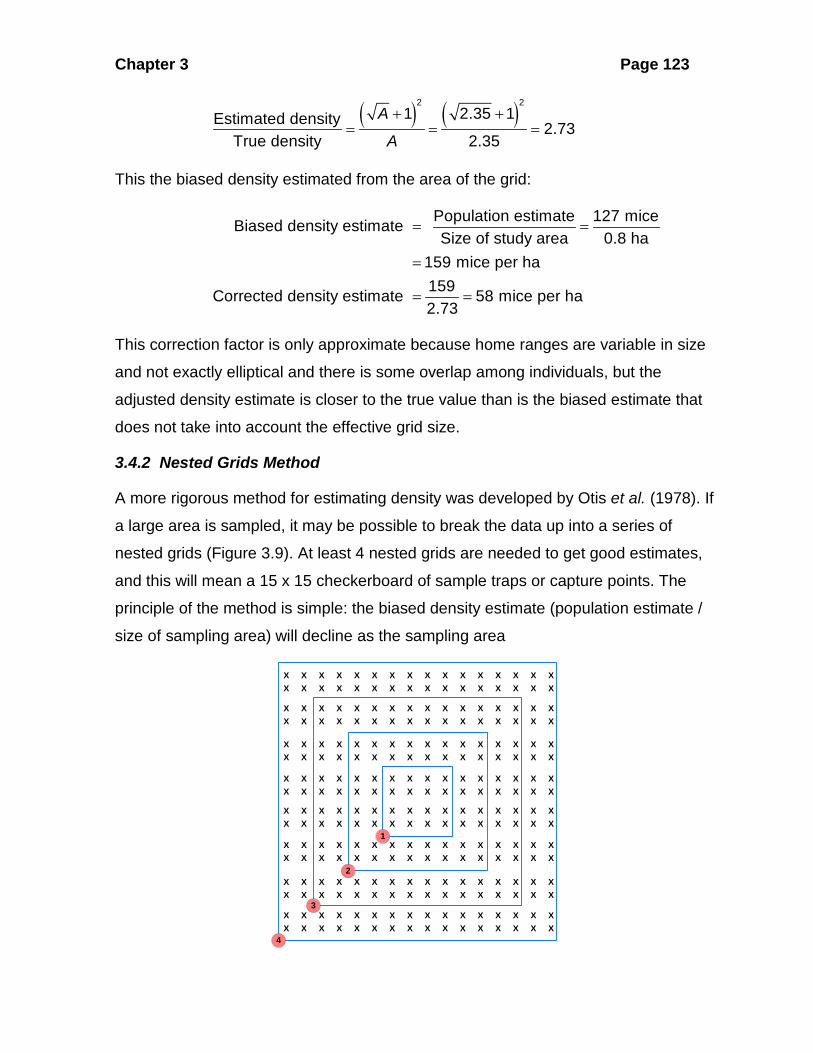
3.4.2 Nested Grids Method
A more rigorous method for estimating density was developed by Otis et al. (1978). If
a large area is sampled, it may be possible to break the data up into a series of
nested grids (Figure 3.9). At least 4 nested grids are needed to get good estimates,
and this will mean a 15 x 15 checkerboard of sample traps or capture points. The
principle of the method is simple: the biased density estimate (population estimate /
size of sampling area) will decline as the sampling area
1
2
3
4 X X X X X X X X X X X X X X X X X X X X X X X X X X X X X X X X
X X X X X X X X X X X X X X X X X X X X X X X X X X X X X X X X
X X X X X X X X X X X X X X X X X X X X X X X X X X X X X X X X
X X X X X X X X X X X X X X X X X X X X X X X X X X X X X X X X
X X X X X X X X X X X X X X X X X X X X X X X X X X X X X X X X
X X X X X X X X X X X X X X X X X X X X X X X X X X X X X X X X
X X X X X X X X X X X X X X X X X X X X X X X X X X X X X X X X
X X X X X X X X X X X X X X X X X X X X X X X X X X X X X X X X
Chapter 3 Page 124
Figure 3.9 An example of a set of nested grids for population density estimation. The entire study area is a 16 x 16 checkerboard, and 4 nested subgrids are shown by the blue lines. The nested grids are 4 x 4, 8 x 8, 12 x 12, and 16 x 16, and if the sample points are 10 m apart (for example), the areas of these four subgrids would be 0.16 ha, 0.64 ha, 1.44 ha, and 2.56 ha.
increases in size. Each nested grid will have a larger and larger area of boundary
strip as grid size increases (Figure 3.9), and we can use the change in observed
density to estimate the width of the boundary strip for the population being studied.
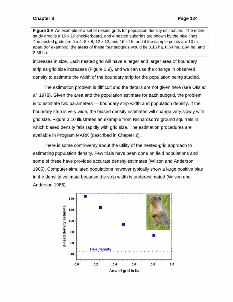
The estimation problem is difficult and the details are not given here (see Otis et
al. 1978). Given the area and the population estimate for each subgrid, the problem
is to estimate two parameters boundary strip width and population density. If the
boundary strip is very wide, the biased density estimates will change very slowly with
grid size. Figure 3.10 illustrates an example from Richardson’s ground squirrels in
which biased density falls rapidly with grid size. The estimation procedures are
available in Program MARK (described in Chapter 2).
There is some controversy about the utility of the nested-grid approach to
estimating population density. Few trials have been done on field populations and
some of these have provided accurate density estimates (Wilson and Anderson
1985). Computer-simulated populations however typically show a large positive bias
in the densi ty estimate because the strip width is underestimated (Wilson and
Anderson 1985).
Area of grid in ha0.0 0.2 0.4 0.6 0.8 1.0
Bia
sed
dens
ity e
stim
ate
40
60
80
100
120
140
True density
Chapter 3 Page 125
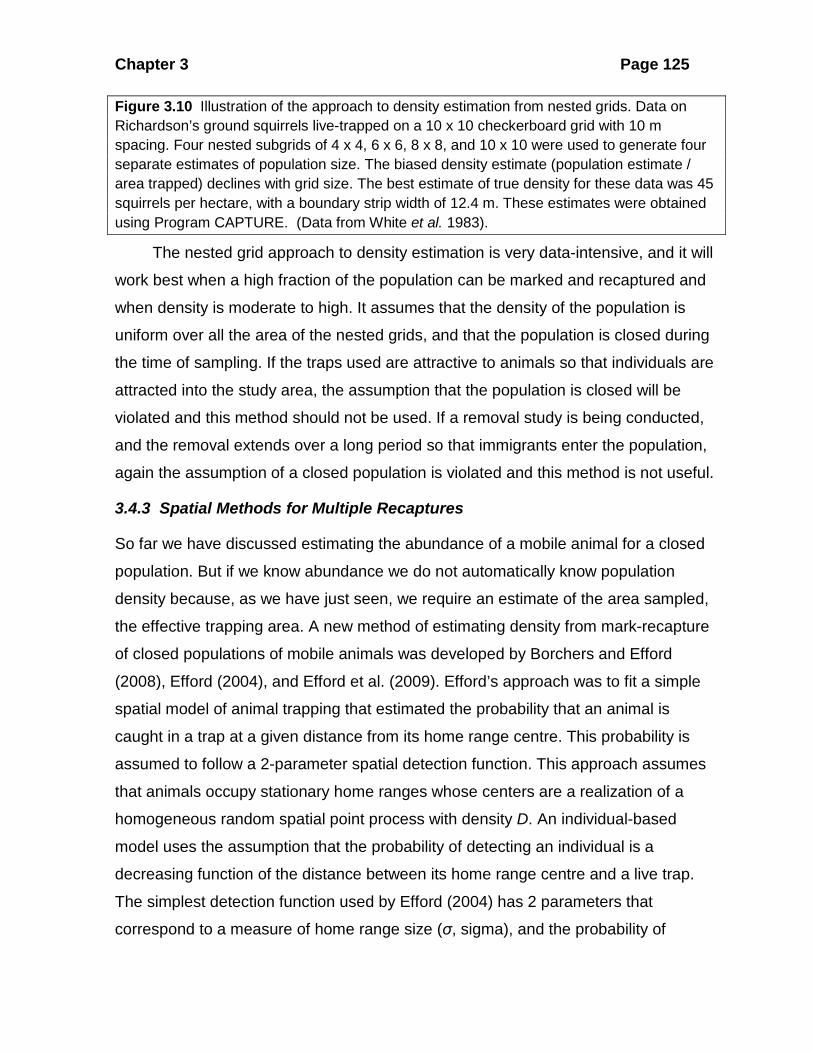
Figure 3.10 Illustration of the approach to density estimation from nested grids. Data on Richardson’s ground squirrels live-trapped on a 10 x 10 checkerboard grid with 10 m spacing. Four nested subgrids of 4 x 4, 6 x 6, 8 x 8, and 10 x 10 were used to generate four separate estimates of population size. The biased density estimate (population estimate / area trapped) declines with grid size. The best estimate of true density for these data was 45 squirrels per hectare, with a boundary strip width of 12.4 m. These estimates were obtained using Program CAPTURE. (Data from White et al. 1983).
The nested grid approach to density estimation is very data-intensive, and it will
work best when a high fraction of the population can be marked and recaptured and
when density is moderate to high. It assumes that the density of the population is
uniform over all the area of the nested grids, and that the population is closed during
the time of sampling. If the traps used are attractive to animals so that individuals are
attracted into the study area, the assumption that the population is closed will be
violated and this method should not be used. If a removal study is being conducted,
and the removal extends over a long period so that immigrants enter the population,
again the assumption of a closed population is violated and this method is not useful.
3.4.3 Spatial Methods for Multiple Recaptures
So far we have discussed estimating the abundance of a mobile animal for a closed
population. But if we know abundance we do not automatically know population
density because, as we have just seen, we require an estimate of the area sampled,
the effective trapping area. A new method of estimating density from mark-recapture
of closed populations of mobile animals was developed by Borchers and Efford
(2008), Efford (2004), and Efford et al. (2009). Efford’s approach was to fit a simple
spatial model of animal trapping that estimated the probability that an animal is
caught in a trap at a given distance from its home range centre. This probability is
assumed to follow a 2-parameter spatial detection function. This approach assumes
that animals occupy stationary home ranges whose centers are a realization of a
homogeneous random spatial point process with density D. An individual-based
model uses the assumption that the probability of detecting an individual is a
decreasing function of the distance between its home range centre and a live trap.
The simplest detection function used by Efford (2004) has 2 parameters that
correspond to a measure of home range size (σ, sigma), and the probability of
Chapter 3 Page 126
capture at the centre of the home range (g0). These 2 parameters can be estimated
from the distances between recaptures of marked animals and the frequency of
capture. The approach used in Efford’s method assumes that the spatial point
process is Poisson, and that the shape of the detection function is either half of a
normal distribution, a negative exponential, or a hazard function.
Two possible methods of estimation of the spatial model have been developed.
Efford (2004) developed the first approach through inverse prediction (IP) and
simulation. A second approach was developed by Borchers and Efford (2008) and
utilizes maximum likelihood methods to derive a better density estimate than is
achieved by inverse prediction. Efford (2009) and Borchers and Efford (2008) used
simulation to demonstrate that the maximum likelihood method gave the most
accurate estimate of true density in comparison to other methods using the boundary
strip approach. The details of the estimation problem are given in Efford (2004) and
Borchers and Efford (2008) and implemented in Program DENSITY 4
(http://www.otago.ac.nz/density/ ).
The data required from a closed population for Program DENSITY are a series
of data on the capture locations for a set of animals (Table 3.3). There must be two or
more capture or live trapping sessions because the key data are measures of the
scale of movements the individuals make. If there are no movements of marked
individuals, the spatial model cannot be used, and the larger the sample of
movements, the more precise the estimated density. A spatial map of the detectors
(e.g. live traps) must also be available. The detectors can be in any spatial format as
long as you have a spatial map of potential detectors (Figure 3.11). In particular the
detectors such as live traps do not need to be in a checkerboard grid pattern like that
shown in Figure 3.7.
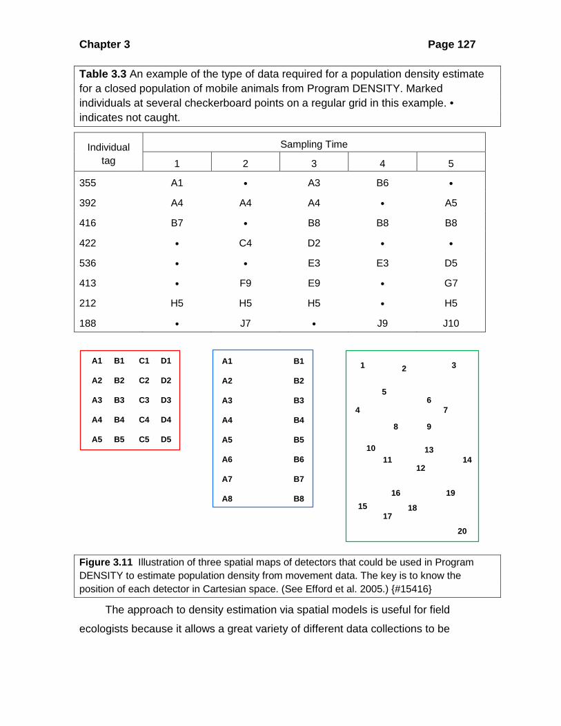
Chapter 3 Page 127
Table 3.3 An example of the type of data required for a population density estimate for a closed population of mobile animals from Program DENSITY. Marked individuals at several checkerboard points on a regular grid in this example. • indicates not caught.
Individual tag
Sampling Time
1 2 3 4 5
355 A1 • A3 B6 •
392 A4 A4 A4 • A5
416 B7 • B8 B8 B8
422 • C4 D2 • •
536 • • E3 E3 D5
413 • F9 E9 • G7
212 H5 H5 H5 • H5
188 • J7 • J9 J10
Figure 3.11 Illustration of three spatial maps of detectors that could be used in Program DENSITY to estimate population density from movement data. The key is to know the position of each detector in Cartesian space. (See Efford et al. 2005.) {#15416}
The approach to density estimation via spatial models is useful for field
ecologists because it allows a great variety of different data collections to be
1 2 3
4
56
7
8 9
1011
12
1314
1516
1718
19
20
B1
B2
B3
B4
B5
B6
B7
B8
A1
A2
A3
A4
A5
A6
A7
A8
A1
A2
A3
A4
A5
B1
B2
B3
B4
B5
C1
C2
C3
C4
C5
D1
D2
D3
D4
D5
Chapter 3 Page 128
analysed. The proximity detectors may be cameras, DNA caught in hair traps,
multiple live-catch traps or single live-catch traps.
I will not try to detail the calculations used in these spatial models because the
mathematics are beyond the scope of this book. Interested students are referred to
Efford et al. (2009){#15413}. Box 3.3 illustrates the data and results from an analysis
of stoat (weasel) DNA collections in New Zealand.
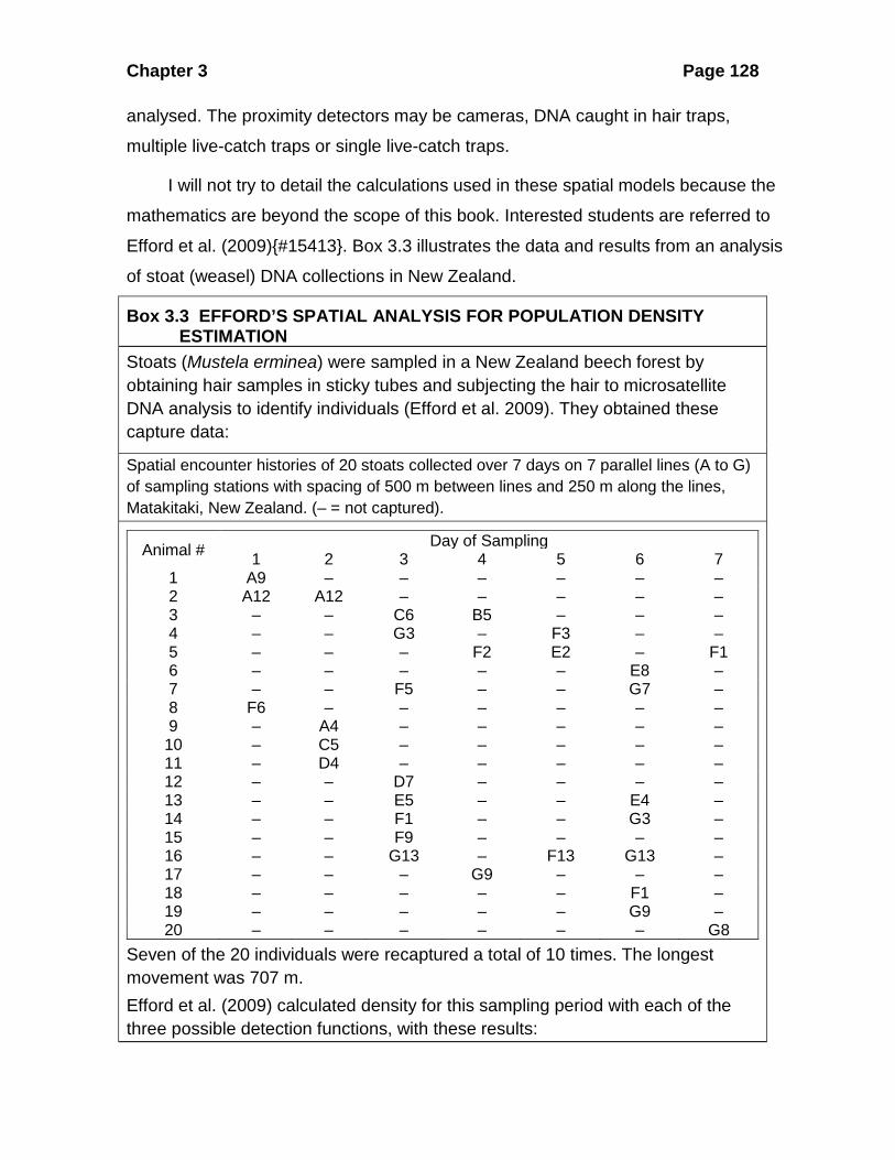
Box 3.3 EFFORD’S SPATIAL ANALYSIS FOR POPULATION DENSITY ESTIMATION
Stoats (Mustela erminea) were sampled in a New Zealand beech forest by obtaining hair samples in sticky tubes and subjecting the hair to microsatellite DNA analysis to identify individuals (Efford et al. 2009). They obtained these capture data:
Spatial encounter histories of 20 stoats collected over 7 days on 7 parallel lines (A to G) of sampling stations with spacing of 500 m between lines and 250 m along the lines, Matakitaki, New Zealand. (– = not captured).
Animal # Day of Sampling 1 2 3 4 5 6 7
1 A9 – – – – – – 2 A12 A12 – – – – – 3 – – C6 B5 – – – 4 – – G3 – F3 – – 5 – – – F2 E2 – F1 6 – – – – – E8 – 7 – – F5 – – G7 – 8 F6 – – – – – – 9 – A4 – – – – – 10 – C5 – – – – – 11 – D4 – – – – – 12 – – D7 – – – – 13 – – E5 – – E4 – 14 – – F1 – – G3 – 15 – – F9 – – – – 16 – – G13 – F13 G13 – 17 – – – G9 – – – 18 – – – – – F1 – 19 – – – – – G9 – 20 – – – – – – G8
Seven of the 20 individuals were recaptured a total of 10 times. The longest movement was 707 m. Efford et al. (2009) calculated density for this sampling period with each of the three possible detection functions, with these results:
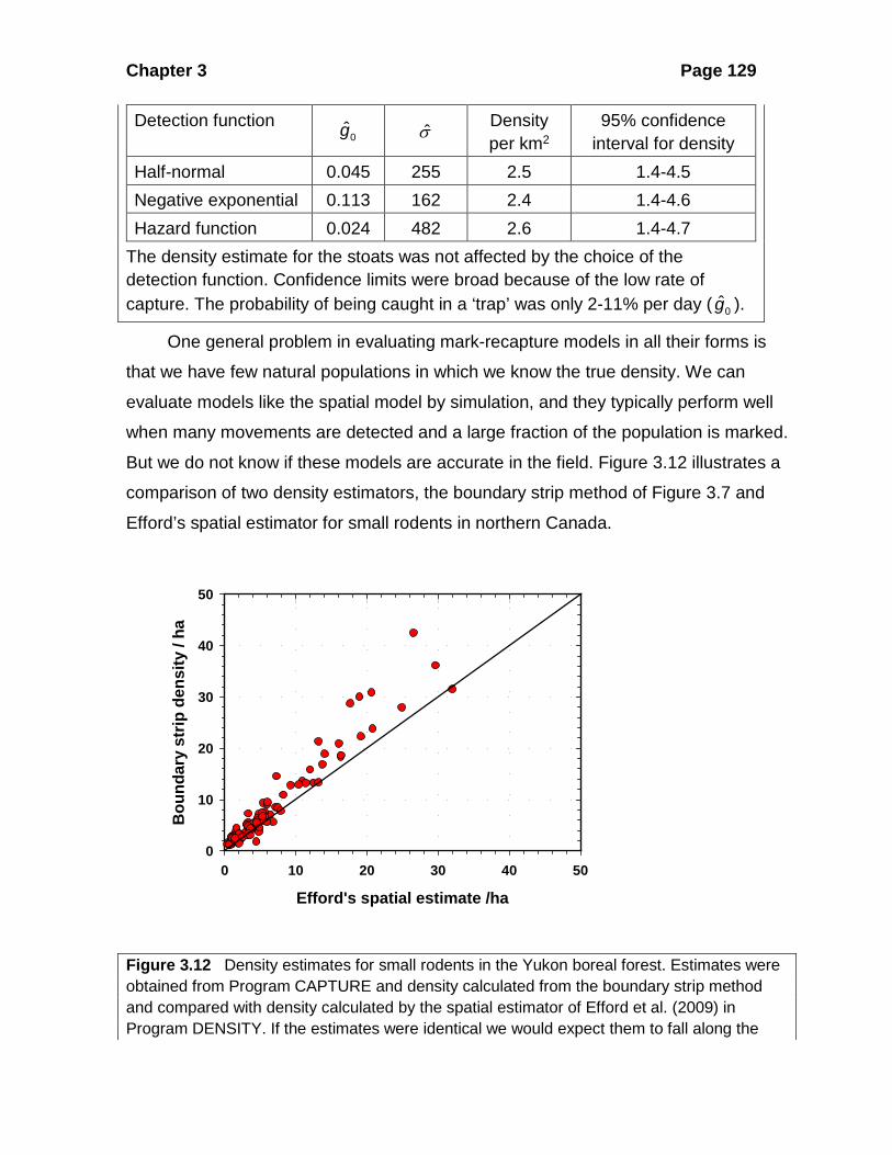
Chapter 3 Page 129
Detection function 0g σ Density
per km2 95% confidence
interval for density Half-normal 0.045 255 2.5 1.4-4.5 Negative exponential 0.113 162 2.4 1.4-4.6 Hazard function 0.024 482 2.6 1.4-4.7
The density estimate for the stoats was not affected by the choice of the detection function. Confidence limits were broad because of the low rate of capture. The probability of being caught in a ‘trap’ was only 2-11% per day ( 0g ).
One general problem in evaluating mark-recapture models in all their forms is
that we have few natural populations in which we know the true density. We can
evaluate models like the spatial model by simulation, and they typically perform well
when many movements are detected and a large fraction of the population is marked.
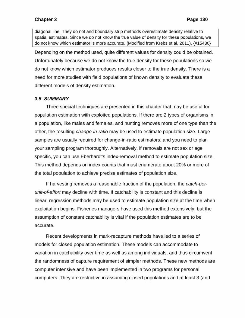
But we do not know if these models are accurate in the field. Figure 3.12 illustrates a
comparison of two density estimators, the boundary strip method of Figure 3.7 and
Efford’s spatial estimator for small rodents in northern Canada.
Boreal forest
Efford's spatial estimate /ha0 10 20 30 40 50
Bou
ndar
y st
rip d
ensi
ty /
ha
0
10
20
30
40
50
Figure 3.12 Density estimates for small rodents in the Yukon boreal forest. Estimates were obtained from Program CAPTURE and density calculated from the boundary strip method and compared with density calculated by the spatial estimator of Efford et al. (2009) in Program DENSITY. If the estimates were identical we would expect them to fall along the
Chapter 3 Page 130
diagonal line. They do not and boundary strip methods overestimate density relative to spatial estimates. Since we do not know the true value of density for these populations, we do not know which estimator is more accurate. (Modified from Krebs et al. 2011). {#15430}
Depending on the method used, quite different values for density could be obtained.
Unfortunately because we do not know the true density for these populations so we
do not know which estimator produces results closer to the true density. There is a
need for more studies with field populations of known density to evaluate these
different models of density estimation.
3.5 SUMMARY Three special techniques are presented in this chapter that may be useful for
population estimation with exploited populations. If there are 2 types of organisms in
a population, like males and females, and hunting removes more of one type than the
other, the resulting change-in-ratio may be used to estimate population size. Large
samples are usually required for change-in-ratio estimators, and you need to plan
your sampling program thoroughly. Alternatively, if removals are not sex or age
specific, you can use Eberhardt’s index-removal method to estimate population size.
This method depends on index counts that must enumerate about 20% or more of
the total population to achieve precise estimates of population size.
If harvesting removes a reasonable fraction of the population, the catch-per-
unit-of-effort may decline with time. If catchability is constant and this decline is
linear, regression methods may be used to estimate population size at the time when
exploitation begins. Fisheries managers have used this method extensively, but the
assumption of constant catchability is vital if the population estimates are to be
accurate.
Recent developments in mark-recapture methods have led to a series of
models for closed population estimation. These models can accommodate to
variation in catchability over time as well as among individuals, and thus circumvent
the randomness of capture requirement of simpler methods. These new methods are
computer intensive and have been implemented in two programs for personal
computers. They are restrictive in assuming closed populations and at least 3 (and
Chapter 3 Page 131
typically 5) capture periods, and they require individual capture histories to be
recorded for all animals.
Enumeration methods have a long history in population ecology and their
simplicity makes them attractive. But all methods of enumeration suffer from a
negative bias population estimates are always less than or equal to the true
population and they should be used only as a last resort. The critical assumption
of enumeration methods is that you have captured or sighted all or nearly all of the
animals in the population, so that the bias is minimal. Enumeration methods may be
required for endangered species which cannot be captured without trauma.
All of the methods in this chapter and the previous chapter estimate population
size, and to convert this to population density you must know the area occupied by
the population. This is simple for discrete populations on islands but difficult for
species that are spread continuously across a landscape. Nested grids may be used
to estimate density, or a boundary strip may be added to a sampling area to
approximate the actual area sampled. Density estimates are more reliable when the
sampling area is large relative to the home range of the animal being studied, and
when a large fraction of the individuals can be captured.
Spatial models have been developed that utilize the movements of marked
individuals in a closed population to estimate density. These methods assume that
individuals have a constant home range size and move independently. They require
a series of 5-10 or more movements for individuals with a trapping session. They
could provide a less biased estimate of density than boundary strip methods, but
more evaluation on field populations of known size is required to determine which
density estimation method is most accurate.
SELECTED READINGS Efford, M.G., Borchers, D.L., and Byrom, A.E. 2009. Density estimation by spatially
explicit capture-recapture: likelihood-based methods. In Modeling Demographic Processes in Marked Populations. Edited by E.G.C. D.L. Thomson, M.J. Conroy. Springer, New York. pp. 255-269.

Chapter 3 Page 132
Foster, R.J., and Harmsen, B.J. 2012. A critique of density estimation from camera-trap data. Journal of Wildlife Management 76(2): 224-236.
Lebreton, J. D. (1995). The future of population dynamics studies using marked individuals: a statistician's perspective. Journal of Applied Statistics 22, 1009-1030.
Matlock, R. B. J., Welch, J. B. & Parker, F. D. (1996). Estimating population density per unit area from mark, release, recapture data. Ecological Applications 6, 1241-1253.
Miller, S. D., White, G. C., Sellers, R. A., Reynolds, H. V., Schoen, J. W., Titus, K., Barnes, V. G., Smith, R. B., Nelson, R. R., Ballard, W. B. & Schwartz, C. C. (1997). Brown and black bear density estimation in Alaska using radiotelemetry and replicated mark-resight techniques. Wildlife Monographs 61, 1-55.
Obbard, M.E., Howe, E.J., and Kyle, C.J. 2010. Empirical comparison of density estimators for large carnivores. Journal of Applied Ecology 47(1): 76-84.
Rosenberg, D. K., Overton, W. S. & Anthony, R. G. (1995). Estimation of animal abundance when capture probabilities are low and heterogeneous. Journal of Wildlife Management 59, 252-261.
Wilson, D.J., Efford, M.G., Brown, S.J., Williamson, J.F., and McElrea, G.J. 2007. Estimating density of ship rats in New Zealand forests by capture-mark-recapture trapping. New Zealand Journal of Ecology 31: 47-59.
Wilson, K. R. & Anderson, D. R. (1985). Evaluation of two density estimators of small mammal population size. Journal of Mammalogy 66, 13-21 {#15420} {#15937} {#15413} { #15990}
QUESTIONS AND PROBLEMS 3.1. For the catch-effort regression estimation technique of Leslie, discuss the type of
bias in estimated population size when there is:
(a) Change in catchability during the experiment
(b) Natural mortality during the experiment.
(c) Mortality caused by the marking procedure or the tag itself.
(d) Emigration of animals from the population.
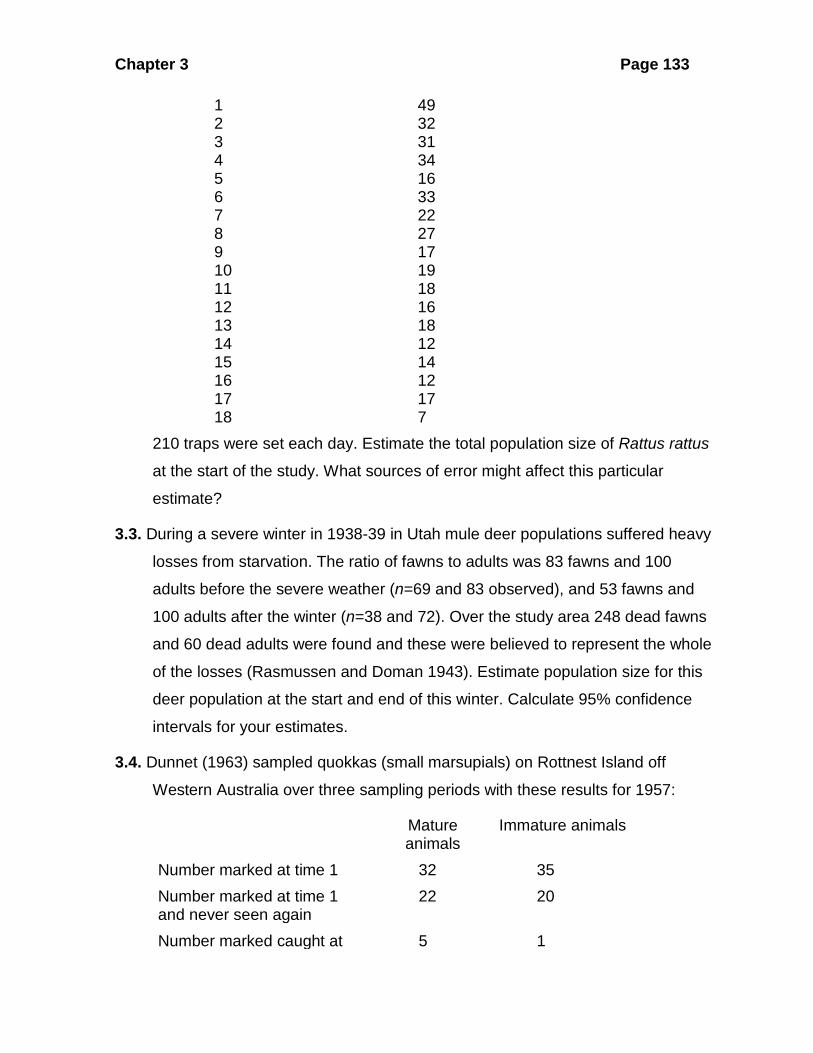
3.2. Leslie and Davis (1939) set 210 rat traps (break-back type) in 70 houses in
Freetown, Sierra Leone in 1937. They caught over 18 days:
Day No. of Rattus rattus caught
Chapter 3 Page 133
1 49 2 32 3 31 4 34 5 16 6 33 7 22 8 27 9 17 10 19 11 18 12 16 13 18 14 12 15 14 16 12 17 17 18 7
210 traps were set each day. Estimate the total population size of Rattus rattus
at the start of the study. What sources of error might affect this particular
estimate?
3.3. During a severe winter in 1938-39 in Utah mule deer populations suffered heavy
losses from starvation. The ratio of fawns to adults was 83 fawns and 100
adults before the severe weather (n=69 and 83 observed), and 53 fawns and
100 adults after the winter (n=38 and 72). Over the study area 248 dead fawns
and 60 dead adults were found and these were believed to represent the whole
of the losses (Rasmussen and Doman 1943). Estimate population size for this
deer population at the start and end of this winter. Calculate 95% confidence
intervals for your estimates.
3.4. Dunnet (1963) sampled quokkas (small marsupials) on Rottnest Island off
Western Australia over three sampling periods with these results for 1957:
Mature animals
Immature animals
Number marked at time 1 32 35 Number marked at time 1 and never seen again
22 20
Number marked caught at 5 1
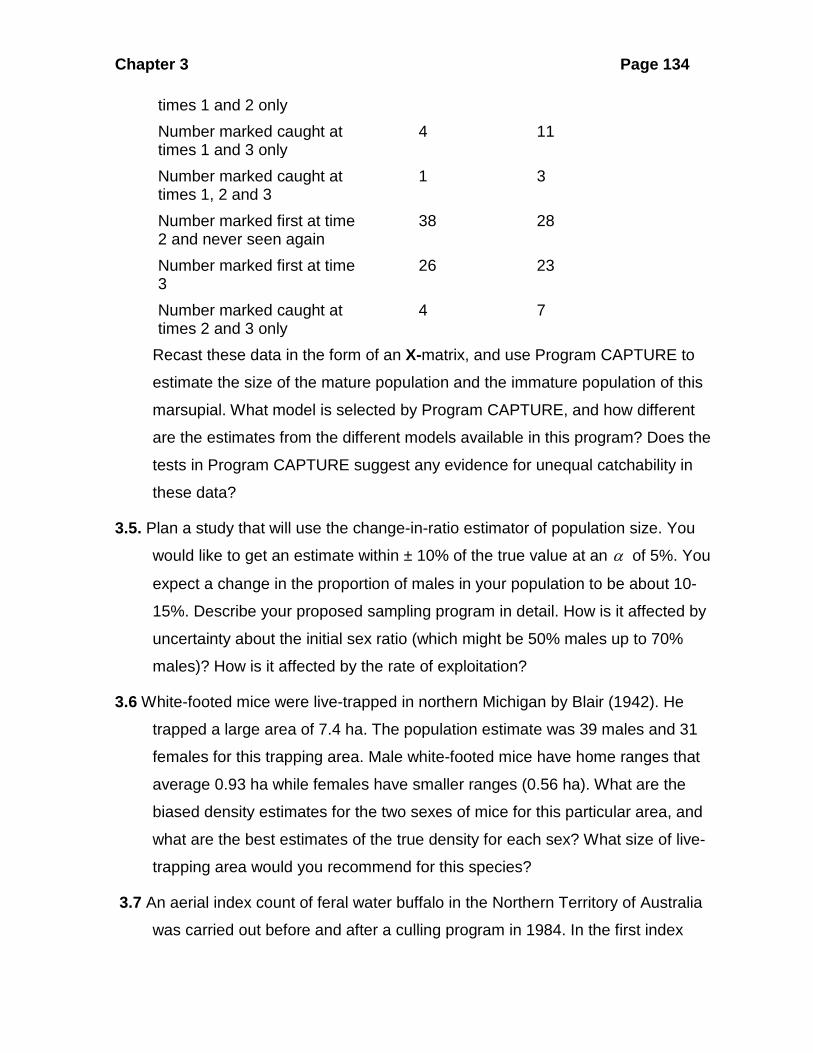
Chapter 3 Page 134
times 1 and 2 only Number marked caught at times 1 and 3 only
4 11
Number marked caught at times 1, 2 and 3
1 3
Number marked first at time 2 and never seen again
38 28
Number marked first at time 3
26 23
Number marked caught at times 2 and 3 only
4 7
Recast these data in the form of an X-matrix, and use Program CAPTURE to
estimate the size of the mature population and the immature population of this
marsupial. What model is selected by Program CAPTURE, and how different
are the estimates from the different models available in this program? Does the
tests in Program CAPTURE suggest any evidence for unequal catchability in
these data?
3.5. Plan a study that will use the change-in-ratio estimator of population size. You
would like to get an estimate within ± 10% of the true value at an α of 5%. You
expect a change in the proportion of males in your population to be about 10-
15%. Describe your proposed sampling program in detail. How is it affected by
uncertainty about the initial sex ratio (which might be 50% males up to 70%
males)? How is it affected by the rate of exploitation?
3.6 White-footed mice were live-trapped in northern Michigan by Blair (1942). He
trapped a large area of 7.4 ha. The population estimate was 39 males and 31
females for this trapping area. Male white-footed mice have home ranges that
average 0.93 ha while females have smaller ranges (0.56 ha). What are the
biased density estimates for the two sexes of mice for this particular area, and
what are the best estimates of the true density for each sex? What size of live-
trapping area would you recommend for this species?
3.7 An aerial index count of feral water buffalo in the Northern Territory of Australia
was carried out before and after a culling program in 1984. In the first index

Chapter 3 Page 135
count 2786 buffalo were counted, and in the second count 1368 were seen. The
cull occurred over two months and 12,890 buffalo were shot. Can you estimate
population size for this population? What proportion of the population was
culled? What assumptions must you make to use these estimates?
3.8. During 7 aerial flights to locate 19 radio-collared caribou in southern British
Columbia over a two week period a total of 144 caribou were seen of which 54
had radio-collars and the remaining 90 were not marked. The frequency of
resighting of the 19 collared caribou were as follows: 7, 5, 1, 2, 3, 0, 5, 3, 1, 3,
0, 2, 4, 6, 1, 5, 1, 3, and 2. Estimate the population size of this caribou herd and
the 90% confidence limits for this estimate.
3.9 Discuss from a practical point of view the advantages and disadvantages of using
a trapping web design versus a nested grid design to estimate population
density for a small mammal. What information might be lost if you adopted one
design over the other?
Recommended