Chapter 21
The open economy and
different exchange rate regimes
In this chapter we consider simple open-economy members of the IS-LM fam-
ily. Section 21.1 revisits the standard static version, the Mundell-Fleming
model, in its fixed-exchange-rate as well as floating-exchange-rate adapta-
tions. The Mundell-Fleming model is well-known from elementary macro-
economics and our presentation of the model is merely a prelude to the next
sections which address dynamic extensions. In Section 21.2 we show how the
dynamic closed-economy IS-LM model with rational expectations from the
previous chapter can be easily modified to cover the case of a small open econ-
omy with fixed exchange rates. In Section 21.3 we go into detail about the
more challenging topic of floating exchange rates. In particular we address
the issue of exchange rate overshooting, first studied by Dornbusch (1976).
Both the original Mundell-Fleming model and the dynamic extensions
considered here are ad hoc in the sense that the microeconomic setting is
not articulated in any precise way. Yet the models are useful and have been
influential as a means of structuring thinking about an open economy in the
short run.
The models focus on short-run mechanisms in a small open economy.
There is a “domestic currency” and a “foreign currency” and these currencies
are traded in the foreign exchange market. In this market, nowadays, the
volume of trade is gigantic.
The following assumptions are shared by the models in this chapter:
1. Perfect mobility across borders of financial capital, but no mobility of
labor.
2. Domestic and foreign bonds are perfect substitutes and command the
same expected rate of return.
793

794
CHAPTER 21. THE OPEN ECONOMY AND DIFFERENT
EXCHANGE RATE REGIMES
3. Domestic and foreign output goods are imperfect substitutes.
4. Nominal prices are sluggish and follow an exogenous constant inflation
path.
As the two last assumptions indicate, we consider an economy with im-
perfectly competitive firms that on and off in an asynchronous way adjust
their prices to unit costs such that within the time horizon of the model the
resulting aggregate inflation rate is sticky.
We use the same notation as in the previous chapter, with the following
clarifications and additions: is domestic output (GDP), the domestic
price level, ∗ the foreign price level, the domestic short-term nominal inter-est rate, ∗ the foreign short-term nominal interest rate, and the nominal
exchange rate. Suppose UK is the “home country”. Then the exchange rate
indicates the price in terms of British£ (GBP) for one US$ (USD), say.
Be aware that the currency trading convention is to announce an exchange
rate as, for example, “ USD/GBP”, meaning by this “USD through GBP
is ” in the sense of GBP per USD. In ordinary language (as well as in
mathematics) a slash, however, means “per”; thus, writing “ USD/GBP”
ought to mean USD per GBP, which is exactly the opposite. Whenever
in this text we use a slash, it has this standard mathematical meaning. To
counter any risk of confusion, when indicating an exchange rate, we therefore
avoid using a slash altogether. Instead we use the unmistakable “per”.1
When reporting that “the exchange rate is ”, our point of view is that
of an importer in the home country. That is, if UK is the “home country”,
saying that “the exchange rate is ” shall mean that GBP must be paid
per $ worth of imports. And saying that “the real exchange rate is ” shall
mean that domestic goods must be paid per imported good. This con-
vention is customary in continental Europe. Note however, that it is the
opposite of the British convention which reports the home country’s nominal
and real “exchange rate” as 1 and 1 respectively.
When considering terms of trade, 1 our point of view is that of an
exporter in the home country. The terms of trade tell us how many foreign
goods we get per exported good. In accordance with this, Box 21.1 gives a
list of key open economy variables.
1Yet another convention is to report an exchange rate this way: “euro against yen is
”. This means euro per yen.
c° Groth, Lecture notes in macroeconomics, (mimeo) 2013.

795
Box 21.1 Open economy glossary
Term Symbol Meaning
Nominal exchange rate The price of foreign currency in terms
of domestic currency.
Real exchange rate ≡∗
The price of foreign goods in terms of
domestic goods (can be interpreted as
an indicator of competitiveness).
Terms of trade 1 In this simple model terms of trade is
just the inverse of the real exchange
rate (generally, it refers to the price of
export goods in terms of import goods).
Purchasing power parity The nominal exchange rate which makes
the cost of a basket of goods and services
equal in two countries, i.e., makes = 1
Uncovered interest parity The hypothesis that domestic and
foreign bonds have the same
expected rate of return, expressed
in terms of the same currency.
Exports
Imports
Net exports (in domestic
output units) = −
Net foreign assets
Net factor income from abroad
(in domestic output units) + The present model has = 0
Current account surplus = + + . In this model = 0
Official reserve assets
Private net foreign assets = −
Increase per time unit
in a variable ∆
Financial account surplus = −∆−∆ = − = current
account deficit.
Net inflow of foreign exchange = = − = − (net outflow offoreign exchange)
We simplify by talking of an exchange rate as if the “foreign country” con-
stitutes the rest of the world and the exchange rate is thereby just a bilateral
entity. A more precise treatment would center on the effective exchange rate,
which is a trade-weighted index of the exchange rate vis-a-vis a collection of
c° Groth, Lecture notes in macroeconomics, (mimeo) 2013.

796
CHAPTER 21. THE OPEN ECONOMY AND DIFFERENT
EXCHANGE RATE REGIMES
major trade partners.
21.1 The Mundell-Fleming model
Whether the Mundell-Fleming model is adapted to a fixed or floating ex-
change rate regime, there is a common set of elements in the framework.
21.1.1 The basic elements
Compared with the static closed-economy IS-LMmodel, theMundell-Fleming
model contains two new elements:
• An extra output demand component, namely a net export function( ) where ≡ ∗ is the real exchange rate. As a higher
income implies more imports, we assume that 0 And as a higher
real exchange rate implies better competitiveness, we assume that
0.2
• The uncovered interest parity condition (for short UIP). This says thatdomestic and foreign financial assets pay the same expected rate of
return (measured in the same currency).
Output demand is given as
= ( ) + ( ) +( ) ++ where (21.1)
0 + ≤ + 1 + ≤ 0 0
and is a demand shift parameter. Disposable income, is
≡ − T (21.2)
where T is real net tax revenue (gross tax revenue minus transfers). Weassume a quasi-linear tax revenue function
T = + ( ) 0 ≤ 0 1 (21.3)
where is a constant representing the “tightness” of fiscal policy. This
parameter, together with the level of public spending, describes fiscal
policy.
2By assuming 0 it is presupposed that the Marshall-Lerner condition is satisfied,
see Appendix A. Throughout the chapter we ignore that it may take one or two years for
a rise in to materialize as a rise in net exports. This is because the price of imports is
immediately increased while the quantity of imports and exports only adjust with a time
lag (the pattern known as the J-curve effect).
c° Groth, Lecture notes in macroeconomics, (mimeo) 2013.

21.1. The Mundell-Fleming model 797
Inserting (21.2) and (21.3) into (21.1), we can write aggregate demand as
= ( ) ++ where (21.4)
0 = (1− 0) + + 1 = + 0
0 = · (−1) ∈ (−1 0)The demand for money (domestic currency and checkable deposits in
commercial banks) in the home country is, as in the closed economy model,
= · (( ) + ) 0 0 (21.5)
where is the short-term nominal interest rate on the domestic bond which
is denominated in the domestic currency. The symbol represents a shift
parameter which may reflect a shock to liquidity preferences or the payment
technology and thereby the money multiplier.
There is a link between and , namely = − where denotes
the expected value of which is the domestic forward-looking inflation rate.
Recall that with continuous interest compounding, the equation = −
is an identity. In a discrete time framework the equation is a convenient
approximation. Assuming clearing in the output market as well as the money
market, we now have:
= ( − ∗
) ++ (IS)
= ( ) + (LM)
In addition to the domestic short-term bond there is a short-term bond
denominated in foreign currency, henceforth the foreign bond. The nominal
interest rate on the foreign bond is denoted ∗ and is exogenous, ∗ 0 Theterm “bonds” may be interpreted in a broad sense, including large firms’
interest-bearing bank deposits.
The no-arbitrage condition between the domestic and the foreign bond is
assumed given by the uncovered interest parity condition,
= ∗ +
(UIP)
where denotes the expected increase per time unit in the exchange rate
in the immediate future.3 The UIP condition says that the interest rate on
3As a preparation for the dynamic extensions to be considered below, we have presented
the UIP condition in its continuous time version with continuous interest compounding.
In discrete time with denoting the exchange rate at the beginning of period the
UIP condition reads: 1 + =1(1 + ∗ )
+1 which can be written 1 + = (1 + ∗ )(1+
(+1 −)) ≈ 1 + ∗ + (
+1 −) when ∗ and (
+1 −) are “small”,
c° Groth, Lecture notes in macroeconomics, (mimeo) 2013.
798
CHAPTER 21. THE OPEN ECONOMY AND DIFFERENT
EXCHANGE RATE REGIMES
the domestic bond is the same as the expected rate of return on investing in
the foreign bond, expressed in the domestic currency. This expected rate of
return equals the foreign interest rate plus the expected rate of depreciation
of the domestic currency.
By invoking the UIP condition the model assumes that risk and liquid-
ity considerations in the choice between domestic and foreign bonds can be
ignored in a first approximation so that domestic and foreign bonds are es-
sentially perfect substitutes. So only the expected rate of return matters. If
we imagine that in the very short run there is, for example, a “” in (UIP)
instead of “=”, then a massive inflow of financial capital will occur, until “=”
in (UIP) is re-established. The adjustment will take the form of a lowering of
in case of a fixed exchange rate system. In case of a floating exchange rate
system the adjustment will take the form of an adjustment in (generally
both its level and subsequent rate of change). Only when (UIP) holds, are
investors indifferent between holding domestic or foreign bonds.
The model assumes that (UIP) holds continuously (arbitrage in interna-
tional asset markets is very fast). Thus, if for example the domestic interest
rate is below the foreign interest rate, it must be that the domestic currency
is expected to appreciate vis-à-vis the foreign currency, that is, 0. The
adjective “uncovered” refers to the fact that the return on the right-hand
side of (UIP) is not guaranteed, but only an expectation.4
The original Mundell-Fleming model is a static model describing just one
short period with the price levels and ∗ set in advance. The model consistsof the equations (IS), (LM), and (UIP) with the following partitioning of the
variables:
• Exogenous: ∗ ∗ and either or
• Endogenous: and either or , depending on the exchange rate
regime.
We now consider the polar cases of fixed and floating exchange rates,
respectively.
21.1.2 Fixed exchange rate
A fixed exchange rate regime amounts to a promise by the central bank to sell
and buy unlimited amounts of foreign currency at an announced exchange
4With uncertainty and absense of risk neutrality added to the model, a risk term
(positive or negative) would have to be added on the right-hand side of (UIP). On the
covered interest parity, see Appendix B.
c° Groth, Lecture notes in macroeconomics, (mimeo) 2013.

21.1. The Mundell-Fleming model 799
rate. So becomes an exogenous constant in the model.5 The system
requires that the central bank keeps foreign exchange reserves to be able
to buy the domestic currency on foreign exchange markets when needed to
maintain its value.
We assume that the announced exchange rate is at a sustainable level vis-
a-vis the foreign currency so that credibility problems can be ignored. So we
let = 0 Then (UIP) reduces to = ∗ and output is determined by (IS),given = ∗. Finally, through movements of financial capital the nominalmoney supply (hence also the real money supply) adjusts endogenously to
the level required by (LM), given = ∗ and the value of already determinedin (IS). The system thus has a recursive structure.
There is no possibility of an independent monetary policy as long as there
are no restrictions on movements of financial capital. The intuition is the
following. Suppose the central bank naively attempts to stimulate output
by buying domestic bonds, thereby raising the money supply. There will
be an incipient fall in . This induces portfolio holders to convert domestic
currency into foreign currency in order to buy foreign bonds and enjoy their
higher interest rate. This tends to raise , however. Assuming the central
bank abides by its commitment to a fixed exchange rate, the bank will have
to immediately counteract this tendency to depreciation by buying domestic
assets (domestic currency and bonds) for foreign currency in an amount
sufficient to bring the domestic money supply down to its original level needed
to restore both the exchange rate and the interest rate at their original values.
That is, as soon as the central bank attempts expansionary monetary policy
it has to reverse it.
The model is qualitatively the same as the static IS-LM model for the
closed economy with the nominal interest rate fixed by the central bank. The
output and money multipliers w.r.t. government spending are, from (IS) and
(LM) respectively,
=
1
1−
=1
1− (1− 0)− −
1
=
=
1
1− (1− 0)− −
0
The output multiplier can be seen as a measure of how much a unit in-
crease in raises aggregate demand and thereby stimulates production and
income; indeed, ∆ ≈ · ∆ = for ∆ = 1. Thereby the
transaction-motivated demand for money is increased. This generates an
5In practice there will be a small margin of allowed fluctuation around the par value.
The Danish krone (DKK) is fixed at 746.036 DKK per 100 euro +/- 2.25 percent.
c° Groth, Lecture notes in macroeconomics, (mimeo) 2013.

800
CHAPTER 21. THE OPEN ECONOMY AND DIFFERENT
EXCHANGE RATE REGIMES
incipient tendency for both the short-term interest rate to rise and the ex-
change rate to appreciate as portfolio holders worldwide buy the currency of
the SOE to invest in its bonds and enjoy their high rate of return. The cen-
tral bank is committed to a fixed exchange rate, however, and has to prevent
the pressure for a higher interest rate and currency appreciation by buying
foreign assets (foreign currency and bonds) for domestic currency. When the
money supply has increased enough to nullify the incipient tendency for a
higher domestic interest rate, the equilibrium with unchanged exchange rate
is restored. The needed increase in the money supply for a unit increase in
is given by ∆ ≈ ·∆ = for ∆ = 1. One may say that
it is the accommodating money supply that allows the full unfolding of the
output multiplier w.r.t. government spending. Nevertheless, owing to the
import leakage ( 0), both the output and money multiplier are lower
than the corresponding multipliers in the closed economy where the central
bank maintains the interest rate at a certain target level. The system ends
up with higher , the same and and lower net exports because of higher
imports.
The output multipliers w.r.t. a demand shock, an interest rate shock,
and a liquidity preference shock, respectively, are
=
=
1
1− (1− 0)− −
1
∗=
1−
= +
1− (1− 0)− −
0
= 0
This last result reflects that after the liquidity preference shock, the money
market equilibrium is restored by full adjustment of the money supply ( =
) at unchanged interest rate.
21.1.3 Floating exchange rate
In a floating exchange rate regime, also called a flexible exchange rate regime,
the exchange rate is allowed to respond endogenously to the market forces,
supply and demand, in the foreign exchange market. The model treats the
money supply, as exogenous. More precisely, the money supply is tar-
geted by the central bank and the model assumes this is done successfully.
The exchange rate adjusts so that the available supplies of money and do-
mestic bonds are willingly held. The primary actors in the foreign exchange
market are commercial banks, asset-management firms, insurance companies,
exporting and importing corporations, and central banks.
c° Groth, Lecture notes in macroeconomics, (mimeo) 2013.

21.1. The Mundell-Fleming model 801
In the present static portrait of the floating exchange rate regime,
is treated as exogenous. Following Mundell (1963), we imagine that the
system has settled down in a steady state with = 0. The model is again
recursive. First (UIP) yields = ∗ Then output is determined by (LM),given = ∗. And finally the required exchange rate is determined by (IS) fora given level of ∗ . So the story behind the equilibrium described by the
model is that the exchange rate has adjusted to a level such that aggregate
demand and output is at the point where, given the real money supply, the
transactions-motivated demand for money establishes money market clearing
for a nominal interest rate equal to the foreign nominal interest rate.
There is no possibility of fiscal policy affecting output as long as there
are no restrictions on movements of financial capital. The interpretation is
the following. Consider an expansive fiscal policy, 0 or 0 The
incipient output stimulation increases the transaction demand for money and
thereby the interest rate. The rise in the interest rate is immediately coun-
teracted, however, by inflow of financial capital induced by the high interest
rate. This inflow raises the demand for the domestic currency, which thereby
appreciates. The appreciation continues until has decreased enough6 to
create a sufficient fall in net exports so that aggregate demand and the in-
terest rate are brought back to their initial levels. In effect the system ends
up with unchanged output and interest rate, a lower exchange rate, and
a lower net exports.7
On the other hand, monetary policy is effective. An increase in the money
supply generates an incipient fall in the interest rate. This triggers a coun-
teracting outflow of financial capital, whereby the domestic currency depre-
ciates, i.e., rises. The depreciation continues until the real exchange rate
has increased enough to induce a rise in net exports and output large enough
for the transaction demand for money to match the larger money supply and
leave the interest rate at its original level. The system ends up with higher
, the same , higher and higher net exports.8
From (LM) and (IS), respectively, we find the output and exchange rate
6Recall that as we have defined the exchange rate, “up is down and down is up”.7This canonical result relies heavily on the assumption that domestic and foreign bonds
are perfect substitutes.8The implicit assumption that a higher does not affect the price level is of course
problematic. If intermediate goods are an important part of imports, then a higher ex-
change rate would imply higher unit costs of production. And since prices tend to move
with costs, this would imply a higher price level. If imports consist primarily of final
goods, however, it is easier to accept the logic of the model.
c° Groth, Lecture notes in macroeconomics, (mimeo) 2013.

802
CHAPTER 21. THE OPEN ECONOMY AND DIFFERENT
EXCHANGE RATE REGIMES
multipliers w.r.t. the money supply:
=
1
0 (21.6)
=
1− (1− 0)− −
∗
0 (21.7)
Finally, the output multipliers w.r.t. a demand shock and a liquidity prefer-
ence shock, respectively, are
=
= 0
= − 1
0
Like increased public spending, a positive output demand shock does not
affect output. It is neutralized by appreciation of the domestic currency.
A positive liquidity preference shock reduces output. The mechanism is
that the increase in money demand triggers an incipient rise in the domestic
interest rate. The concomitant appreciation of the currency, resulting from
the induced inflow of financial capital, reduces net exports.
21.1.4 Perspectives
Ignoring the limitations of this simple static model, its message is that for
a small open economy, a fixed exchange rate regime is better at stabilizing
output if money demand shocks dominate, and a floating exchange rate sys-
tem is better if most shocks are output demand shocks. In any case, there
is an asymmetry. Under a fixed exchange rate system, two macroeconomic
short-run policy instruments are given up: exchange rate policy and mone-
tary policy. Under a floating exchange rate system, only one macroeconomic
short-run policy instrument is given up: fiscal policy. Yet, the historical
experience seems to be that an international system of floating exchange
rates ends up with higher volatility in both real and nominal exchange rates
(Mussa, 1990; Obstfeld and Rogoff, 1996; Basu and Taylor, 1999).
The result that fiscal policy is impotent in the floating exchange rate
regime does not necessarily go through in more general settings. For ex-
ample, in practice, domestic and foreign financial claims may often not be
perfect substitutes. Indeed, the UIP hypothesis is empirically rejected at
short forecast horizons, although it does somewhat better at horizons longer
than a year (see the literature notes at the end of this chapter). And as
already hinted at, treating the price level as exogenous when import prices
change is not satisfactory.
c° Groth, Lecture notes in macroeconomics, (mimeo) 2013.
21.2. Dynamics under a fixed exchange rate 803
Anyway, even the static Mundell-Fleming model provides a basic insight:
the impossible trinity. A society might want a system with the following
three characteristics:
• free mobility of financial capital (to improve resource allocation);• independent monetary policy (to allow a stabilizing role for the centralbank);
• fixed exchange rate (to avoid exchange rate volatility).
But it can have only two of them. A fixed exchange rate system is incom-
patible with the second characteristic. And a flexible exchange rate system
contradicts the third.
In the next sections we extend the model with dynamics and rational
expectations. We first consider the fixed exchange rate regime, next the
flexible exchange rate regime.
21.2 Dynamics under a fixed exchange rate
We ignore the shift parameters and On the other hand we introduce
an additional asset, a long-term bond that is indexed w.r.t. domestic infla-
tion. In the fixed exchange rate regime this extension is easy to manage. In
addition we assume rational expectations. The formal structure of the model
then becomes exactly the same as that of the dynamic IS-LM model for a
closed economy with short- and long-term bonds, studied in the previous
chapter.
With denoting the real long-term interest rate at time (defined as the
internal real rate of return on an inflation indexed consol), aggregate demand
is
= (
) + ( ) +( ) + ≡ ( ) +
where
0 = (1− 0) + + 1 = + 0 0
−1 = − 0
where is the real exchange rate, ∗ with representing the given and
constant nominal exchange rate and the price ratio ∗ assumed constant.
The latter assumption is equivalent with assuming the domestic inflation rate
to equal the foreign inflation rate for all . Moreover, this common inflation
rate is assumed equal to a constant,
c° Groth, Lecture notes in macroeconomics, (mimeo) 2013.
804
CHAPTER 21. THE OPEN ECONOMY AND DIFFERENT
EXCHANGE RATE REGIMES
To highlight the dynamics between fast-moving asset markets and slower-
moving goods markets, the model replaces (IS) by the error-correction spec-
ification
≡
= (
− ) = (( ) +− ) 0 0 given,
(21.8)
where 0 is the constant adjustment speed. Because changing the level
of production is time consuming, 0 is historically given.
We assume the fixed exchange rate policy is sustainable. That is, the
level of is such that no threatening cumulative current account deficits
in the future are glimpsed. In view of rational expectations we then have
= 0 for all ≥ 0 In effect the uncovered interest parity condition reduces
to
= ∗ (21.9)
where the exogenous foreign interest rate, ∗ is for simplicity assumed con-stant.
The remaining elements of the model are well-known from Chapter 20:
= ( ∗) 0 0 (21.10)
=1
(21.11)
1 +
= (21.12)
≡ ∗ − ≡
(21.13)
= 0 (21.14)
where is the real price of the long-term bond (the consol), the superscript
denotes expected value. If a shock occurs, it fits intuition best to interpret
the time derivatives in (21.8), (21.12), and (21.13) as right-hand derivatives,
e.g., ≡ lim∆→0+( (+∆)− ())∆ The variables ∗ 0 and are exogenous constants. The first five of these are positive, and we assume
∗.As there is no uncertainty in this model (no stochastic elements), the
assumption of rational expectations amounts to perfect foresight. We thus
have = and = for all . Therefore, the equations (21.13) and (21.9)
imply = = ∗− 0 for all . Combining this with (21.11) and (21.12),
we end up with
= ( − ∗ + ) (21.15)
c° Groth, Lecture notes in macroeconomics, (mimeo) 2013.
21.2. Dynamics under a fixed exchange rate 805
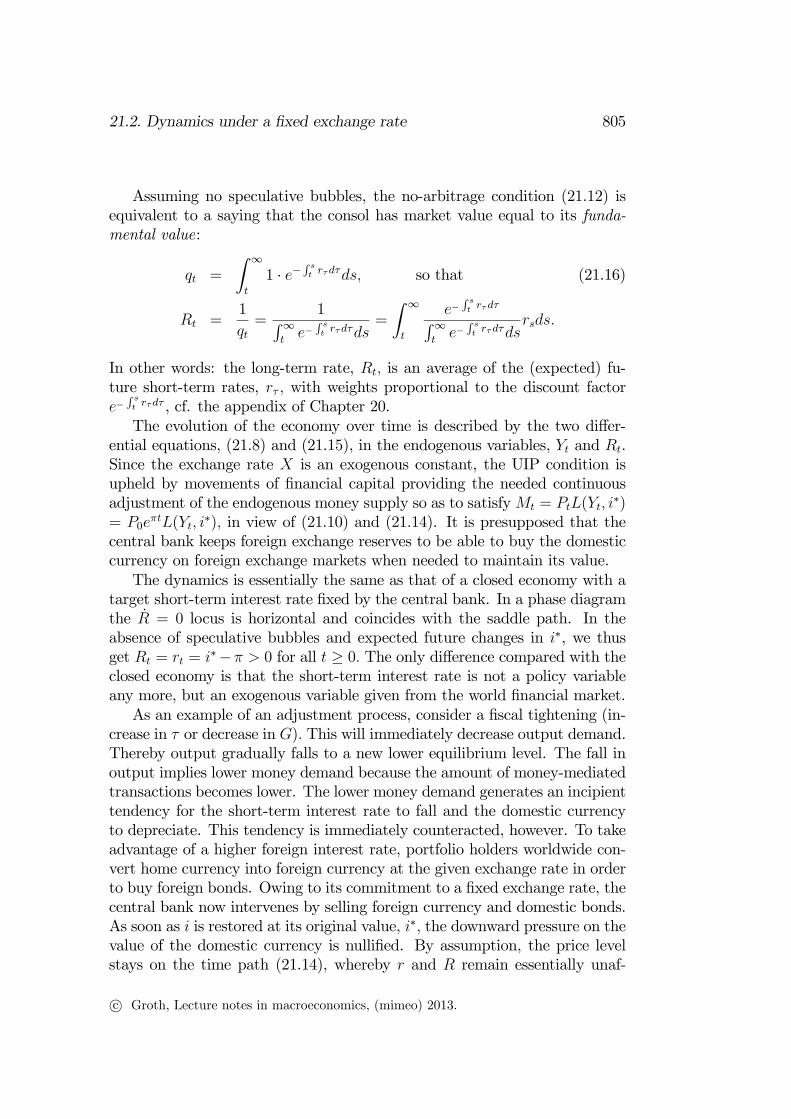
Assuming no speculative bubbles, the no-arbitrage condition (21.12) is
equivalent to a saying that the consol has market value equal to its funda-
mental value:
=
Z ∞
1 · − so that (21.16)
=1
=
1R∞
−
=
Z ∞
− R∞
−
In other words: the long-term rate, is an average of the (expected) fu-
ture short-term rates, with weights proportional to the discount factor
− , cf. the appendix of Chapter 20.
The evolution of the economy over time is described by the two differ-
ential equations, (21.8) and (21.15), in the endogenous variables, and .
Since the exchange rate is an exogenous constant, the UIP condition is
upheld by movements of financial capital providing the needed continuous
adjustment of the endogenous money supply so as to satisfy = ( ∗)
= 0(
∗) in view of (21.10) and (21.14). It is presupposed that thecentral bank keeps foreign exchange reserves to be able to buy the domestic
currency on foreign exchange markets when needed to maintain its value.
The dynamics is essentially the same as that of a closed economy with a
target short-term interest rate fixed by the central bank. In a phase diagram
the = 0 locus is horizontal and coincides with the saddle path. In the
absence of speculative bubbles and expected future changes in ∗, we thusget = = ∗− 0 for all ≥ 0 The only difference compared with theclosed economy is that the short-term interest rate is not a policy variable
any more, but an exogenous variable given from the world financial market.
As an example of an adjustment process, consider a fiscal tightening (in-
crease in or decrease in ) This will immediately decrease output demand.
Thereby output gradually falls to a new lower equilibrium level. The fall in
output implies lower money demand because the amount of money-mediated
transactions becomes lower. The lower money demand generates an incipient
tendency for the short-term interest rate to fall and the domestic currency
to depreciate. This tendency is immediately counteracted, however. To take
advantage of a higher foreign interest rate, portfolio holders worldwide con-
vert home currency into foreign currency at the given exchange rate in order
to buy foreign bonds. Owing to its commitment to a fixed exchange rate, the
central bank now intervenes by selling foreign currency and domestic bonds.
As soon as is restored at its original value, ∗ the downward pressure on thevalue of the domestic currency is nullified. By assumption, the price level
stays on the time path (21.14), whereby and remain essentially unaf-
c° Groth, Lecture notes in macroeconomics, (mimeo) 2013.

806
CHAPTER 21. THE OPEN ECONOMY AND DIFFERENT
EXCHANGE RATE REGIMES
fected and equal to the constant ∗ − during the output contraction. The
figures 20.12 and 20.13 of the previous chapter illustrate .
21.3 Dynamics under a floating exchange rate:
overshooting
The exogeneity − and in fact absence − of expected exchange rate changesin the static Mundell-Fleming model of a floating exchange rate regime is
unsatisfactory. By a dynamic approach we can open up for an endogenous
and time-varying .
The floating exchange rate regime requires one more differential equation
compared to the fixed exchange rate system. To avoid the complexities of
a three-dimensional dynamic system, we therefore simplify along another
dimension by dropping the distinction between short-term and long-term
bonds. Hence, output demand is again described as in (21.1) and depends
negatively on the expected short-term real interest rate, We ignore the
disturbance term .
Apart from the exchange rate now being endogenous, money supply ex-
ogenous, and long-term bonds absent, the model is similar to that of the pre-
vious section. At the same time the model is close to a famous contribution
by the German-American economist Rudiger Dornbusch (1942-2002), who
introduced forward-looking rational expectations into a floating exchange
rate model (Dornbusch, 1976). Dornbusch thereby showed that exchange
rate “overshooting” could arise. This was seen as a possible explanation of
the rise in both nominal and real exchange rate volatility during the 1970s
after the demise of the Bretton-Woods system. In his original article Dorn-
busch wanted to focus on the dynamics between fast moving asset prices
and sluggishly changing goods prices and assumed output to be essentially
unchanged in the process. In the influential Blanchard and Fischer (1989)
textbook this was modified by letting output adjust gradually to spending,
while goods prices follow an exogenous path. This seems a more apt approx-
imation, since the empirics tell us that in response to demand shifts, output
moves faster than goods prices. We follow this approach and name it the
Blanchard-Fischer version of Dornbusch’s overshooting model.
c° Groth, Lecture notes in macroeconomics, (mimeo) 2013.
21.3. Dynamics under a floating exchange rate: overshooting 807
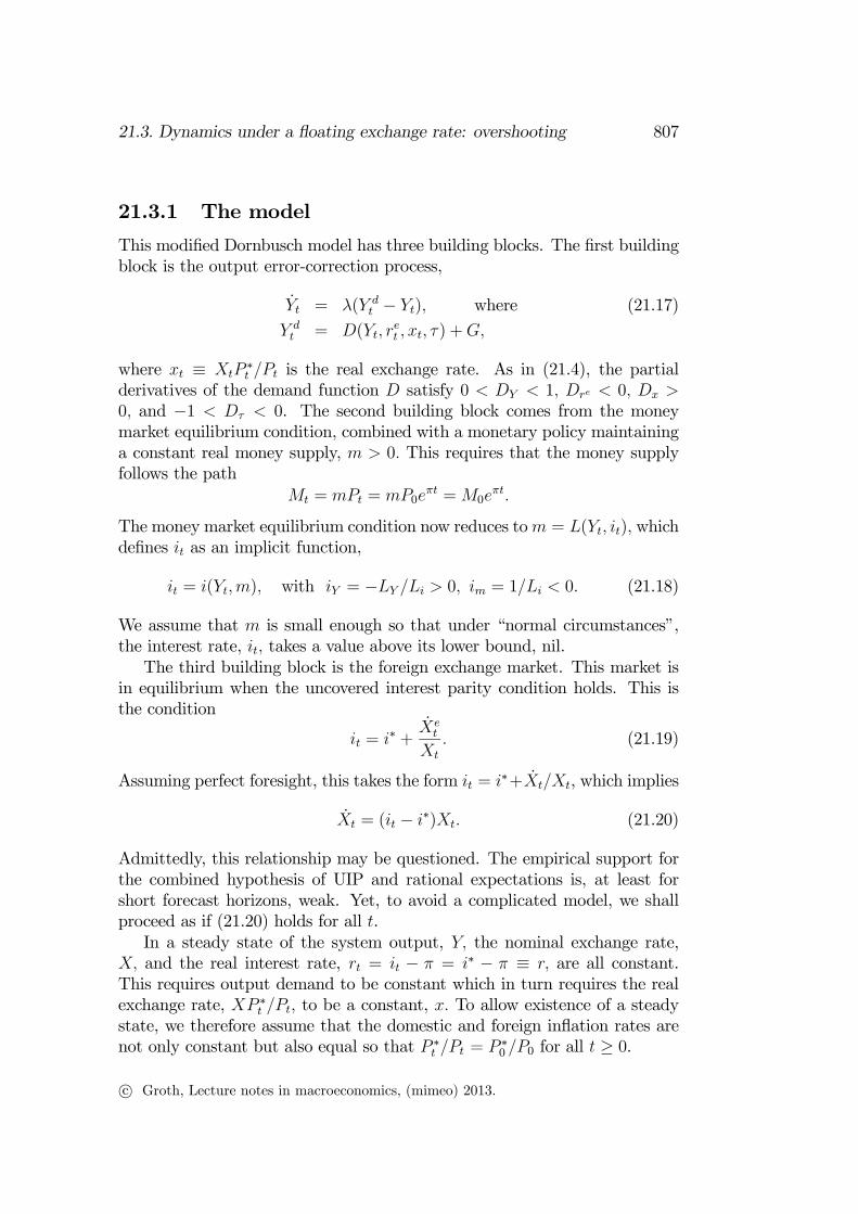
21.3.1 The model
This modified Dornbusch model has three building blocks. The first building
block is the output error-correction process,
= ( − ) where (21.17)
= (
) +
where ≡ ∗ is the real exchange rate. As in (21.4), the partial
derivatives of the demand function satisfy 0 1 0
0 and −1 0. The second building block comes from the money
market equilibrium condition, combined with a monetary policy maintaining
a constant real money supply, 0 This requires that the money supply
follows the path
= = 0 =0
The money market equilibrium condition now reduces to = ( ) which
defines as an implicit function,
= () with = − 0 = 1 0 (21.18)
We assume that is small enough so that under “normal circumstances”,
the interest rate, takes a value above its lower bound, nil.
The third building block is the foreign exchange market. This market is
in equilibrium when the uncovered interest parity condition holds. This is
the condition
= ∗ +
(21.19)
Assuming perfect foresight, this takes the form = ∗+, which implies
= ( − ∗) (21.20)
Admittedly, this relationship may be questioned. The empirical support for
the combined hypothesis of UIP and rational expectations is, at least for
short forecast horizons, weak. Yet, to avoid a complicated model, we shall
proceed as if (21.20) holds for all .
In a steady state of the system output, the nominal exchange rate,
and the real interest rate, = − = ∗ − ≡ are all constant.
This requires output demand to be constant which in turn requires the real
exchange rate, ∗ to be a constant, To allow existence of a steady
state, we therefore assume that the domestic and foreign inflation rates are
not only constant but also equal so that ∗ = ∗0 0 for all ≥ 0.
c° Groth, Lecture notes in macroeconomics, (mimeo) 2013.

808
CHAPTER 21. THE OPEN ECONOMY AND DIFFERENT
EXCHANGE RATE REGIMES
Y
E
0Y
Y
X
X
0X
0Y
A
Figure 21.1: Phase diagram in case of a a floating exchange rate.
Because of perfect foresight, = and = = − for all ≥ 0In view of these conditions together with (21.18), output demand can be
written
= ( ()−
∗00
) + (21.21)
Inserting this into (21.17) and then (21.18) into (21.20), we end up with the
dynamic system
=
∙( ()−
∗00
) +−
¸ 0 0 given,(21.22)
= [()− ∗] (21.23)
This system has and as endogenous variables, whereas the remaining
variables are exogenous and constant: ∗0 0 and ∗ all positiveThe phase diagram is shown in Fig. 21.1. By (21.22), the = 0 locus
is given by the equation = ( ()− ∗0 0 ) +. Taking the
differential on both sides w.r.t. and (for later use) gives
= ( + ) ++
∗00
⇒
(1− − ) = +
∗00
(21.24)
c° Groth, Lecture notes in macroeconomics, (mimeo) 2013.

21.3. Dynamics under a floating exchange rate: overshooting 809
Setting = 0, we find
|=0 =
1− −
∗0 0
0 (21.25)
It follows that the = 0 locus (the “IS curve”) is upward-sloping as shown
in Fig. 21.1.
Equation (21.23) implies that = 0 for () = ∗ The value of satisfying this equation is unique (because 6= 0) and is called That is,
= 0 for = which says that the = 0 locus (the “LM curve”) is
vertical. Fig. 21.1 also indicates the direction of movement in the different
regions, as determined by (21.22) and (21.23). The arrows show that the
steady state is a saddle point. This implies that exactly two solution paths
− one from each side − converge towards E.Since the adjustment of output takes time, is a predetermined variable.
Thus, at time = 0 the economy must be somewhere on the vertical line
= 0. If speculative exchange rate bubbles are assumed away, the explosive
or implosive paths of in Fig. 21.1 cannot arise. Hence, we are left with
the segment AE of the saddle path in the figure as the unique solution to
the model for ≥ 0. Following this path the economy gradually approachesthe steady state E. If 0 (as in Fig. 21.1), output is decreasing and the
exchange rate increasing during the adjustment process. If instead 0 ,
the opposite movements occur.
The steady state can be seen as a “short-run equilibrium” of the economy.
Further dynamic interactions will tend to arise in the “medium run”, for
instance through a Phillips curve and through investment resulting in build
up of fixed capital. These ramifications are ignored by the model.
How the steady state and the = 0 and = 0 loci depend on
In steady state we have
= ( ∗ − ∗00
) + (21.26)
and
= ( ∗) (21.27)
First, (21.27) determines as an implicit function of and ∗ independentlyof (21.26). To see how is affected by a change in we take the differential
on both sides of (21.27) to get = +∗With ∗ = 0 this gives
=
1
0 (21.28)
c° Groth, Lecture notes in macroeconomics, (mimeo) 2013.

810
CHAPTER 21. THE OPEN ECONOMY AND DIFFERENT
EXCHANGE RATE REGIMES
Given we have determined by (21.26). Then, to see how is
affected by a change in we take the differential on both sides of (21.26)
to get = +∗0 0 Combining this with (21.28), we end up
with
=
=
1−
∗0 0
1
0 (21.29)
The intuitive explanation of this sign is linked to that of (21.28). For the
higher money supply to be demanded with unchanged interest rate, equilib-
rium in the money market requires a higher level of transactions, that is, a
higher level of economic activity. In steady state this must be balanced by
a sufficiently higher output demand. And since the marginal propensity to
spend is less than one ( 1), higher net exports are needed; otherwise the
rise in output demand is smaller than the rise in output. Thus, higher com-
petitiveness and therefore depreciation of the domestic currency is required
which means a higher .
Taking into account that = we see that the steady state
multipliers of and w.r.t. are the same as the corresponding multipliers
in the static model, given in (21.6) and (21.7).
It follows from (21.28) that an increase in will shift the = 0 line to
the right, cf. Fig. 21.2. Again, for a higher money supply to be matched
by higher money demand at an unchanged interest rate, a higher level of
economic activity is needed.
As to the effect of higher on the = 0 locus, consider as fixed at
0, i.e., = 0 Then (21.24) gives
|=0=0 = −
∗0 0
= −
∗0 0
0
Hence, an increase in shifts the = 0 locus downward. The intuition is
that a rise in induces a fall in the interest rate; then for output demand
to remain unchanged, we need an appreciation, i.e., a fall in .
Another way of understanding the shift of the = 0 locus is to consider
as fixed at 0 i.e., = 0 Then (21.24) yields
|=0=0
=
1− −=
1− +
0 (21.30)
Hence, we can also say that an increase in shifts the = 0 locus rightward,
cf. Fig. 21.2. The intuition is that, given the fall in induced by higher
increases output demand and therefore also the output level that matches
output demand.
c° Groth, Lecture notes in macroeconomics, (mimeo) 2013.

21.3. Dynamics under a floating exchange rate: overshooting 811
The conclusion is that a higher shifts both the = 0 locus and the
= 0 locus rightward. Then it might seem ambiguous in what direction
moves. But we already know from (21.29) that will unambiguously
increase. The explanation is that, first, a higher output level is needed for
money market equilibrium to obtain. Second, for the higher output level to
be demanded, we need a depreciation of the domestic currency, i.e., a higher
. Fig. 21.2 illustrates.
21.3.2 Unanticipated rise in the real money supply
Now, we are ready to study the dynamic effects of an unanticipated upward
shift in the real money supply, Suppose the economy has been in its steady
state until time 0 Then unexpectedly a discrete open market purchase by
the central bank of domestic bonds takes place. This instantly increases the
monetary base which through the money multiplier leads to a larger money
stock and a smaller stock of bonds held by the private sector. At the same
time the nominal interest rate jumps down because output, and thereby
the volume of transactions, is given in this “very short run” (it takes time
to change output). The lower interest rate prompts an (actual or at least
potential) outflow of financial capital sufficiently large to make the exchange
rate jump up to a level from which it is expected to appreciate at a rate
such that interest parity is reestablished. Very fast, a new “very-short-run”
equilibrium is formed where the given supplies of money and domestic bonds
are willingly held by the agents.9 The essence of the matter is that for a while
we have ∗ due to the increase in the money supply. Hence expectedappreciation is needed to make domestic bonds equally attractive as foreign
bonds. This requires an initial depreciation in excess of that implied by the
new steady state.
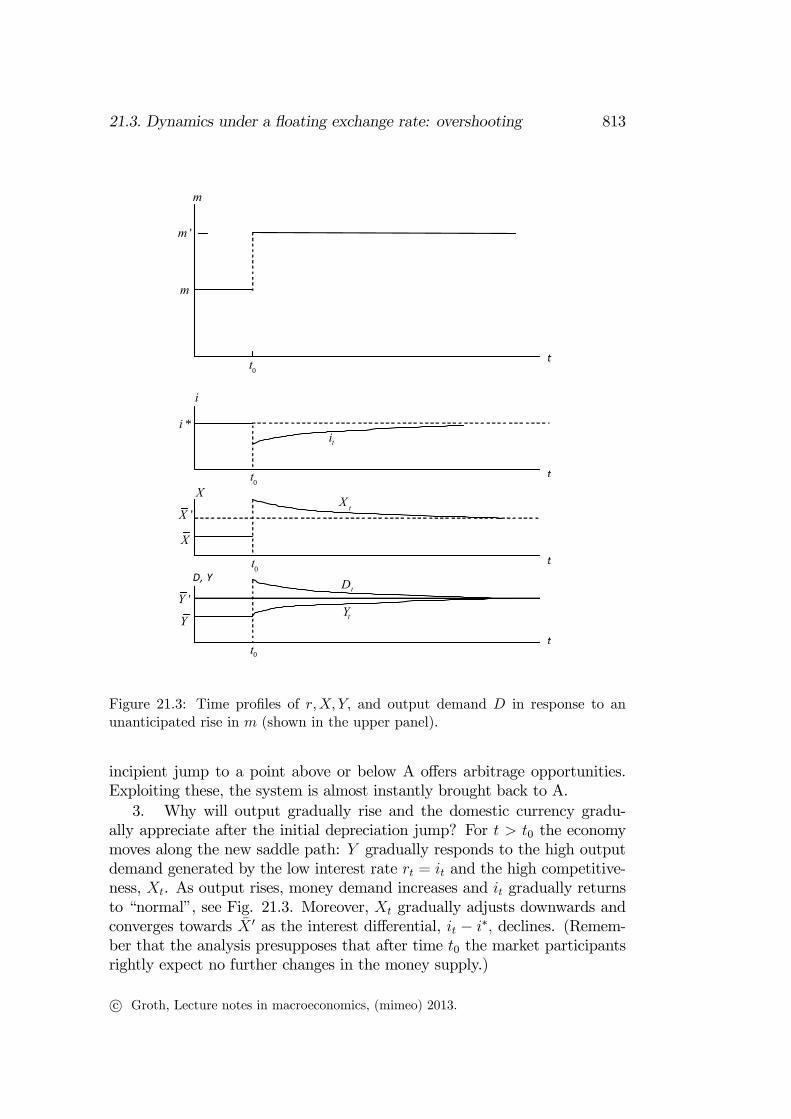
Fig. 21.2 illustrates this exchange rate “overshooting”. We say that a
variable overshoots if its initial reaction to a shock is greater than its longer-
run response. Fig. 21.3 shows the time profiles of the exchange rate and the
other key variables ( is output demand).
To really understand what is going on, let us examine the mechanics of
overshooting more closely:
1. What will be the new steady state expected by the market partici-
pants? As we have just seen, when increases, both the = 0 locus and
the = 0 locus move to the right. The = 0 locus moves to the right,
because the higher tends to decrease so that an offsetting increase in
9The demand for foreign bonds has also changed (increased), but by definition of a
small open economy, this effect is imperceptible and ∗ remains the same.
c° Groth, Lecture notes in macroeconomics, (mimeo) 2013.
812
CHAPTER 21. THE OPEN ECONOMY AND DIFFERENT
EXCHANGE RATE REGIMES
E
0new Y
Y
X
X
0new X
E’ 'X
A
'YY
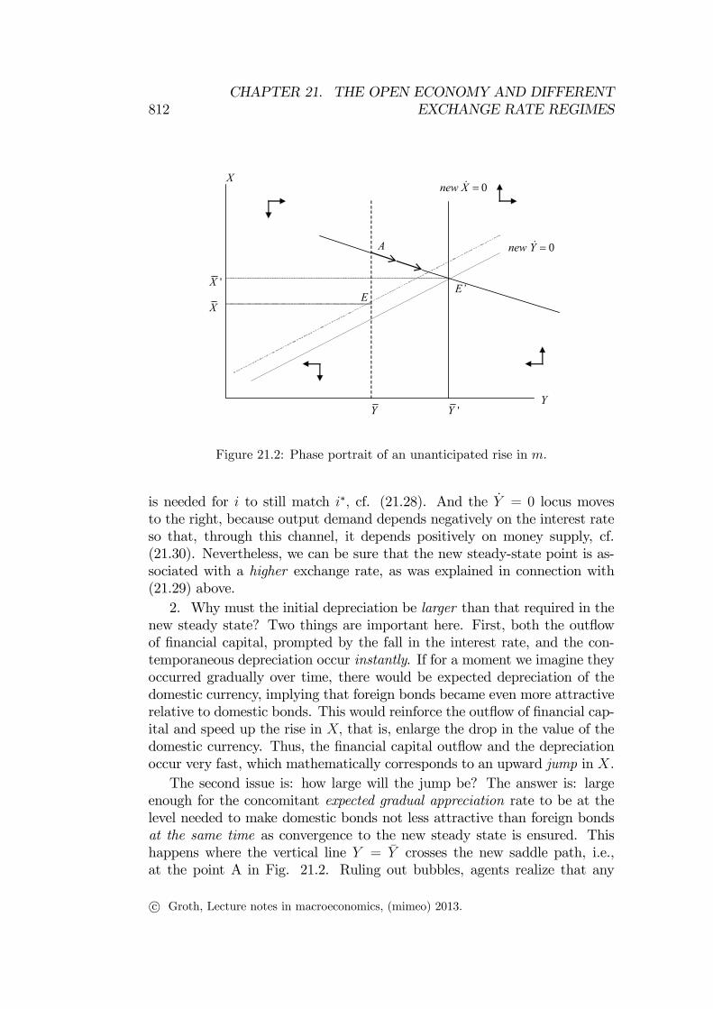
Figure 21.2: Phase portrait of an unanticipated rise in
is needed for to still match ∗ cf. (21.28). And the = 0 locus moves
to the right, because output demand depends negatively on the interest rate
so that, through this channel, it depends positively on money supply, cf.
(21.30). Nevertheless, we can be sure that the new steady-state point is as-
sociated with a higher exchange rate, as was explained in connection with
(21.29) above.
2. Why must the initial depreciation be larger than that required in the
new steady state? Two things are important here. First, both the outflow
of financial capital, prompted by the fall in the interest rate, and the con-
temporaneous depreciation occur instantly. If for a moment we imagine they
occurred gradually over time, there would be expected depreciation of the
domestic currency, implying that foreign bonds became even more attractive
relative to domestic bonds. This would reinforce the outflow of financial cap-
ital and speed up the rise in that is, enlarge the drop in the value of the
domestic currency. Thus, the financial capital outflow and the depreciation
occur very fast, which mathematically corresponds to an upward jump in .
The second issue is: how large will the jump be? The answer is: large
enough for the concomitant expected gradual appreciation rate to be at the
level needed to make domestic bonds not less attractive than foreign bonds
at the same time as convergence to the new steady state is ensured. This
happens where the vertical line = crosses the new saddle path, i.e.,
at the point A in Fig. 21.2. Ruling out bubbles, agents realize that any
c° Groth, Lecture notes in macroeconomics, (mimeo) 2013.
21.3. Dynamics under a floating exchange rate: overshooting 813
t
i
*i
ti
t
X
'X
X
0t
0t
D, Y
tX
0t t
Y
'Y tY
tD
t0
t
m
'm
m
Figure 21.3: Time profiles of and output demand in response to an
unanticipated rise in (shown in the upper panel).
incipient jump to a point above or below A offers arbitrage opportunities.
Exploiting these, the system is almost instantly brought back to A.
3. Why will output gradually rise and the domestic currency gradu-
ally appreciate after the initial depreciation jump? For 0 the economy
moves along the new saddle path: gradually responds to the high output
demand generated by the low interest rate = and the high competitive-
ness, . As output rises, money demand increases and gradually returns
to “normal”, see Fig. 21.3. Moreover, gradually adjusts downwards and
converges towards 0 as the interest differential, − ∗ declines. (Remem-ber that the analysis presupposes that after time 0 the market participants
rightly expect no further changes in the money supply.)
c° Groth, Lecture notes in macroeconomics, (mimeo) 2013.

814
CHAPTER 21. THE OPEN ECONOMY AND DIFFERENT
EXCHANGE RATE REGIMES
The exchange rate as a forward-looking variable
It helps the interpretation of the dynamics if we recognize that the exchange
rate is an asset price, hence forward-looking. Under perfect foresight the un-
covered interest parity implies that the exchange rate satisfies the differential
equation (21.23), except at points of discontinuity of For convenience we
repeat the differential equation here:
= ( − ∗) (21.31)
For fixed 0 we can write the solution of this linear differential equation
as
= (−∗) ≡
(_
−∗)(−) for
where_
is the mean of the interest rates between time and time i.e.,_
≡ R
(− ) Being a forward-looking variable, is not predetermined.
It is therefore more natural to write the solution on the forward-looking form
= −
(−∗) ≡
−(_
−∗)(−) for (21.32)
where and should be interpreted as the expected future values as seen
from time . Thus, under the UIP hypothesis the exchange rate today equals
the expected future exchange rate discounted by the mean interest differential_
− ∗ expected to be in force in the meantime.10 As a consequence, newinformation implying anticipation of a higher in the future (compared
with the reference path) will, for given expectations as to the mean interest
differential show up immediately as depreciation of the domestic currency
today.
From our explanation of the mechanics of overshooting the reader might
think that financial capital movements that prompt an exchange rate ad-
justment require a lot of exchange transactions to occur. All that is needed,
however, for expected asset returns to be equalized is that the traders in
response to new information adjust their bid and ask prices to the new level
where supply and demand of the different assets are equilibrated. In this way,
what we see need not be more than an international re-evaluation of financial
claims and liabilities. In highly integrated asset markets a new equilibrium
may be found quite fast. These circumstances notwithstanding, the volume
of foreign exchange trading per day has in recent years grown to enormous
magnitudes.
10The solution formula (21.32) presupposes absence of any jump in between time
and time . Or more to the point: arbitrage prevents any such expected jump. Ex post,
the formula (21.32) is valid only if no jumps in actually occurred in the time interval
considered.
c° Groth, Lecture notes in macroeconomics, (mimeo) 2013.
21.3. Dynamics under a floating exchange rate: overshooting 815
Returning to our specific case of a monetary expansion, let → ∞ in
(21.32) to get
= lim→∞
−
(−∗) = 0−
∞(−∗) 0 (21.33)
where the new steady-state value of the exchange rate after the rise in is
denoted 0 as in Fig. 21.3. The inequality in (21.33) is due to ∗ duringthe adjustment process. As time proceeds, the shortfall of the domestic vis-
à-vis the foreign interest rate is reduced and the exchange rate converges
to its steady-state value from above. When for instance 90% of the initial
distance from the steady state has been recovered, we say that the system
has essentially reached its steady state. The adjustment process so far may
not involve more time than a couple of years, say. Several factors that may
matter for further adjustments are ignored by this model. Hence, we avoid
to call 0 a “long-run” value.In (21.32) and (21.33) we consider the value of the foreign currency in
terms of the domestic currency. Similar expressions of course hold for the
value of the domestic currency in terms of the foreign currency. Thus, in-
verting (21.32) gives
−1 = −1
− (∗−) ≡ −1
−(∗−
_
)(−)
That is, the value of the domestic currency today equals its expected future
value discounted by the mean interest differential ∗ −_
expected to be in
force in the meantime. Inverting (21.33) yields
−1 = 0−1−
∞(∗−) 0−1
As time proceeds, the excess of the foreign over the domestic interest rate
decreases and the value of the domestic currency converges to its steady-state
value from below.
21.3.3 Anticipated rise in the money supply
As an alternative scenario suppose that the economy has been in steady
state until time 0 when agents suddenly become aware that an increase in
the money supply is going to take place at some future time. To be specific
let us imagine that the central bank at time 0 credibly announces that there
will be discrete upward shift in at time 1 0 while for a long time
after 1 will grow at the same rate, as before. According to the model this
credible announcement immediately causes a jump in the exchange rate
in the same direction as the longer-run change, that is, a jump to some level
c° Groth, Lecture notes in macroeconomics, (mimeo) 2013.

816
CHAPTER 21. THE OPEN ECONOMY AND DIFFERENT
EXCHANGE RATE REGIMES
X
'X
E
0new Y
Y
X 0new X
E’
A
'YY
C
B BX
Figure 21.4: Phase portrait of an anticipated rise in
like in Fig. 21.4. This is due to the agents’ anticipation that after time
1, the economy will be on the new saddle path. Or, in more economic terms,
the agents know that (a) from time 1, the expansionary monetary policy will
cause the interest rate to be lower than ∗, and (b) the exchange rate musttherefore at time 1 have reached a level from which it can have an expected
and actual rate of appreciation such that interest parity is maintained in
spite of ∗ after time 1.Under these circumstances, at the old exchange rate, there would
be excess supply of domestic bonds and excess demand for foreign bonds
immediately after time 0 and this is what instantly triggers the jump to
After this initial jump the exchange rate, will adjust continuously.
Currency is an asset, hence anticipated discrete jumps in the exchange rate
are ruled out by arbitrage. In particular, at time 1 there can be no jump,
because no new information has arrived.
In the time interval (0 1) the movement of () is governed by the
“old” dynamics. That is, for 0 1 the economy must follow a tra-
jectory consistent with the “old” dynamics, reflecting the operation of the
no-arbitrage condition,
() = ∗ +
which rules as long as the announced policy change is not yet implemented.
Under perfect foresight, the market mechanism “selects” that trajectory (
c° Groth, Lecture notes in macroeconomics, (mimeo) 2013.

21.3. Dynamics under a floating exchange rate: overshooting 817
in Fig. 21.4) along which it takes exactly 1− 0 time units to reach the new
saddle path. It is in fact this requirement that determines the size of the
jump in immediately after time 011
The higher competitiveness caused by the instantaneous depreciation im-
plies higher output demand, so that output begins a gradual upward adjust-
ment already before monetary policy has been eased. Along with the rising
, transaction demand for money rises gradually and so do the interest rate
(recall has not changed yet) and the exchange rate. That is, in the time
interval (0 1) we have both ∗ and 0 so as to maintain interest
parity. The process continues until the new monetary policy is implemented
at time 1 Exactly at this time the economy’s trajectory, governed by the
old dynamic regime, crosses the new saddle path, cf. the point in Fig.
21.4. The actual rise in = at time 1 then triggers the anticipated
discrete fall in the interest rate to a level 1 ∗.12 For 1 the economy
features gradual appreciation ( 0) during the adjustment along the new
saddle path. Although output demand is therefore now falling, it is still high
enough to pull output further up until the new steady state E’ is reached.
The time profiles of , and (= ) are shown in Fig. 21.5. The
tangent to the curve at = 0 is horizontal. Hence, infinitely close to 0the size of is vanishing. This is dictated by the “old dynamics” ruling in
the time interval (0 1) which entail that the trajectory through the point B
in Fig.21.4 is horizontal at B. And this is in accordance with interest parity
since it takes time for to rise above hence for to rise above ∗ Notealso that if the length of the time interval (0 1) were small enough, then
might already immediately after time 0 be above its new steady-state level,
0. However, Fig. 21.4 and Fig. 21.5 depict the opposite case, where thetime interval (0 1) is somewhat larger.
21.3.4 Monetary policy tightening
Considering an downward shifts in the money supply path, the above processes
are reversed.
11The level can be shown to be unique and this is also what intuition tells us.
Imagine that the jump, − was smaller than in Fig. 21.4. Then, not only would
there be a longer way along the road to the new saddle path, but the system would also
start from a position closer to the steady state point E, which implies an initially lower
adjustment speed.12Since right before 1 we have ∗ one might wonder whether the fall in the interest
rate is necessarily large enough to ensure ∗ right after 1 The fall is, indeed, largeenough because the dynamics in the time interval (0 1) ensures 1 0 from which
follows (1 0) ( 00) = ∗ where the inequality is due to 0
c° Groth, Lecture notes in macroeconomics, (mimeo) 2013.

818
CHAPTER 21. THE OPEN ECONOMY AND DIFFERENT
EXCHANGE RATE REGIMES
t
0t
m
'm
m
t
i
*i
ti
t
X
'X
X
0t
0t
D, Y
tX
0t
t
Y
'Y
tY
tD
1t
1t
1t
1t
Figure 21.5: Time profiles of and output demand in response to an
anticipated rise in (shown in the upper panel).
c° Groth, Lecture notes in macroeconomics, (mimeo) 2013.
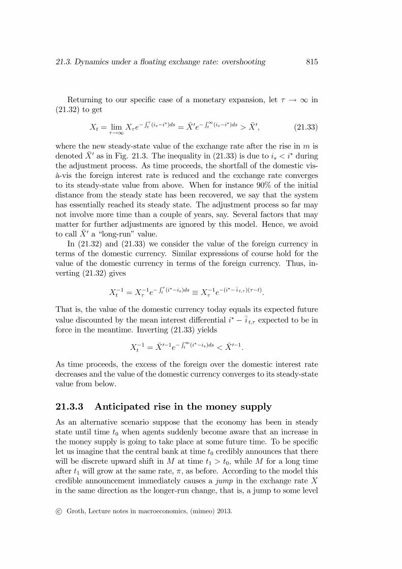
21.3. Dynamics under a floating exchange rate: overshooting 819
'Y
E’
new 0Y
Y
X
X ’
0new X
Y
A
EX
Figure 21.6: Phase portrait of an unanticipated fall in
Unanticipated monetary policy tightening
Suppose the system is in steady state until time 0 Then, unexpectedly, a
discrete open market sale by the central bank of domestic bonds takes place.
The new steady state will have a lower exchange rate. Indeed, given the
lower money supply and unchanged interest rate, equilibrium in the money
market requires a lower level of transactions, that is, a lower level of economic
activity. In steady state this must be balanced by a sufficiently lower output
demand. And since the marginal propensity to spend is less than one (
1), lower net exports are needed; otherwise the fall in output demand is
smaller than the fall in output. Thus, lower competitiveness and therefore
appreciation of the domestic currency is required which means a lower .
In the short run, the nominal interest rate jumps up, prompting an inflow
of financial capital, which in turn prompts a jump down in the exchange
rate, as shown in Fig. 21.6. This appreciation must be large enough to
generate the expected rate of depreciation required for domestic bonds to
be no more attractive than foreign bonds in spite of ∗ Very fast anew “very-short-run” equilibrium is formed where the supplies of money
and bonds are willingly held by the agents. The fact that there must be
expected depreciation is the reason that an initial appreciation in excess of
that implied by the new steady-state equilibrium is required. Again the
c° Groth, Lecture notes in macroeconomics, (mimeo) 2013.

820
CHAPTER 21. THE OPEN ECONOMY AND DIFFERENT
EXCHANGE RATE REGIMES
Figure 21.7: Time profiles of and in response to an unanticipated fall in
(shown in the upper panel).
c° Groth, Lecture notes in macroeconomics, (mimeo) 2013.

21.3. Dynamics under a floating exchange rate: overshooting 821
X
'Y
E’
new 0Y
Y
X ’
0new X
Y
B
E X
C
Figure 21.8: Phase portrait of an anticipated fall in .
exchange rate “overshoots”, this time by taking a greater downward jump
than corresponding to the new steady-state level.
For 0 the economy moves along the new saddle path: gradually
rises and gradually falls in response to the low output demand generated
by the high interest rate = − and the low competitiveness, In the
process, money demand decreases and gradually returns to “normal”, see
Fig. 21.7. Moreover, gradually adjusts upwards and converges towards
0 as the interest differential, − ∗ gradually vanishes.
Anticipated monetary policy tightening
It may happen that the public in advance have a feeling that a monetary
policy shift is on the way, due to foreseeable overheating problems, say. To
be more specific, suppose that at time 0 a tightening of monetary policy is
credibly announced by the central bank to be implemented at time 1 0in the form of a reduction in real money supply to the level 0
Fig. 21.8 illustrates what happens from time 0. As soon as the future
tight monetary policy becomes anticipated, there is an immediate effect on
in the same direction as the “longer-run” effect, i.e., drops to some
point as in Fig. 21.8. Indeed, agents anticipate that from time 1 the tight
monetary policy will cause the interest rate to be higher than ∗, therebyengendering gradual depreciation (rise in ) along the new saddle path.
Arbitrage prevents any anticipated discrete jump in the exchange rate after
c° Groth, Lecture notes in macroeconomics, (mimeo) 2013.

822
CHAPTER 21. THE OPEN ECONOMY AND DIFFERENT
EXCHANGE RATE REGIMES
Figure 21.9: Time profiles of and in response to an anticipated fall in
(shown in the upper panel).
c° Groth, Lecture notes in macroeconomics, (mimeo) 2013.

21.4. Concluding remarks 823
time 0
In the time interval (0 1) the economy must follow a trajectory consis-
tent with the “old” dynamics. The market mechanism “selects” that trajec-
tory ( in Fig. 21.8) along which it takes exactly 1−0 time units to reachthe new saddle path. The lower competitiveness caused by the instantaneous
appreciation implies lower output demand, so that output begins a gradual
downward adjustment already before monetary policy has been tightened.
The time profiles of , and = − are shown in Fig. 21.9. If the
length of the time interval (0 1) is small enough, may already immedi-
ately after time 0 be below its new steady-state level. However, Fig. 21.8
and Fig. 21.9 depict the opposite case, where the time interval (0 1) is
somewhat larger.
21.4 Concluding remarks
The dynamic model of a floating exchange rate regime shows that with fast
moving asset markets and sticky inflation, large volatility in exchange rates
can occur. And large volatility of both nominal and real exchange rates under
a floating exchange rate regime is in fact what the data show. Nevertheless,
there are empirical problems with the model. One of them is that it seems
to exaggerate the exchange rate fluctuations (see Obstfeld and Rogoff, 1996,
p. 621 ff.). Moreover, several empirical studies reject the UIP condition or at
least they reject the combined hypothesis of UIP and rational expectations
(Lewis 1995).
In the model versions considered here the price level moves along a fixed
path. An extended model should incorporate that the domestic price level de-
pends on import prices and that persistent changes in aggregate production
and employment are likely to activate an expectations-augmented Phillips
curve. As they stand, the models imply that monetary shocks have perma-
nent real effects, contrary to what the data in general indicates.
Incorporating a medium-run equilibrium level of the real exchange rate,
anchored by some kind of expected purchasing power parity, opens up for
interesting issues. With ∗ denoting a medium-run equilibrium real exchangerate, 0 in (21.33) would equal ∗( ∗) where ( ∗) is the expectedmedium-run value of the relative price level ∗ Then, suppose the interestrate differential suddenly rises because the foreign country (the U.S., say)
is hit by an economic recession. According to (21.33), this immediately
triggers an appreciation of the home currency (China, say). Alternatively,
imagine that the expected long-run value of ∗ goes down due to a strongproductivity development in the domestic economy. According to (21.33),
c° Groth, Lecture notes in macroeconomics, (mimeo) 2013.

824
CHAPTER 21. THE OPEN ECONOMY AND DIFFERENT
EXCHANGE RATE REGIMES
also this triggers an appreciation of the home currency (China, say).
21.5 Literature notes
(incomplete)
The origin of the Mundell-Fleming model goes back to Robert Mundell
(1963, 1964) and Marcus Fleming (1962). The over-shooting hypothesis:
Dornbusch (1976). What we named the Blanchard-Fischer version of Dorn-
busch’s overshooting model was presented in the Blanchard and Fischer
(1989) textbook. At one point our adaptation departs from Blanchard and
Fischer, who ignore the negative dependence of output demand on the in-
terest rate. Though recognizing this dependency makes the analysis slightly
more cumbersome, it is worth the trouble as it strengthens the results.
An extensive treatment of open economy macroeconomics is contained in
the textbook Obstfeld, M., and K. Rogoff, 1996, Foundations of International
Macroeconomics, The MIT Press, London. In Chapter 8 the authors discuss
the empirical difficulty that the UIP condition is rejected at short prediction
horizons although it does somewhat better at horizons longer than one year.
Other textbook treatments of this empirical issue include:
Feenstra and Taylor (2012).
Krugman, Obstfeld, and Melitz (2012).
Wickens, M., 2008, Macroeconomic Theory. A Dynamic General Equi-
librium Approach, Princeton University Press, Oxford, Ch. 11.4.
Advanced approaches:
Frydman, R., and M. Goldberg, ?.
Isard, P., 2008, “Uncovered interest parity”. In: The new Palgrave Dictio-
nary of Economics. Second edition. Online: http://www.econ.ku.dk/English/
libraries/links/
Lewis, K. K., 1995, Puzzles in international financial markets. In: Hand-
book of International Economics, vol. III, Elsevier, Amsterdam.
The volume of foreign exchange trading per day has in recent years in-
creased to enormous magnitudes. This fact indicates that differences in in-
formation and expectations are prevalent. Recent contributions in macroeco-
nomic theory and empirics are considering how to incorporate heterogeneity,
imperfect knowledge, and agent’s uncertainty about what is the right model
of the economy. See e.g. Ellison ( ).
c° Groth, Lecture notes in macroeconomics, (mimeo) 2013.

21.6. Appendix 825
21.6 Appendix
A. The Marshall-Lerner condition
By assuming that net exports depends positively on the real exchange rate
( 0) the Mundell-Fleming model presupposes that the Marshall-Lerner
condition is satisfied. This is the condition that the weighted sum of the
absolute elasticities of exports and imports w.r.t. the real exchange rate is
large enough to offset the decrease in the terms of trade implied by a higher
real exchange rate. If in the initial situation, net exports are zero, then the
sum of the two absolute elasticities should be above 1. The econometric
evidence is that the condition is satisfied for industrialized countries if we
allow for an adjustment period of one to two years (Artus and Knight, 1984,
Table 4, cf. Krugman, Obstfeld, and Melitz, 2012, p. 492). It may be argued
that there should be a countervailing effect of the real exchange rate, in
the consumption function since the purchasing power of domestic income is
eroded by an increase in The Mundell-Fleming model assumes that the
effect of this on aggregate demand is dominated by the role of 0
B. The covered interest parity
When buying foreign bonds one can avoid the uncertainty concerning the
future exchange rate by entering a forward exchange deal with someone else.
An investor in foreign bonds may thus today contract with her bank to sell
in thirty days a certain amount of foreign currency for domestic currency at
a pre-specified rate. This rate is called the thirty-day forward exchange rate.
It is generally different from the spot exchange rate, But empirically the
two move closely together.
The covered interest parity condition, CIP, is the associated no-arbitrage
condition. In discrete time it reads:
1 + =1
(1 + ∗ )+1 (CIP)
where+1 is the one-period forward exchange rate. If there is no default risk
and no fear that regulations will be imposed which restrain the movement of
foreign funds, arbitrage will immediately make CIP hold. Indeed, an agent
can borrow one unit of the domestic currency, buy 1 units of the foreign
currency, for this amount buy foreign one-period bonds paying a return of
1 + ∗ per bond after one period, and then lock in the future payout in thedomestic currency by selling the return forward at the rate
+1 As the
whole undertaking can be conducted at time there is no risk.
c° Groth, Lecture notes in macroeconomics, (mimeo) 2013.
826
CHAPTER 21. THE OPEN ECONOMY AND DIFFERENT
EXCHANGE RATE REGIMES
Let us compare with the (UIP) in discrete time:
1 + =1
(1 + ∗ )+1 (UIP)
We see that the UIP will hold if and only if +1 =
+1 But to the extent
that riskiness of foreign currencies plays a role, the forward exchange rate
will differ from the expected. So UIP will no longer hold.
21.7 Exercises
c° Groth, Lecture notes in macroeconomics, (mimeo) 2013.
Recommended