26
Chapter 2
REGIONS AND THE ZPL LANGUAGE
This chapter describes the ZPL language, concentrating on the role of regions in its
design. To make this discussion both readable and precise, some language concepts are
introduced informally at first and are then reconsidered with increased formality as the
chapter progresses. While this format would not be appropriate for a language reference
manual, it is designed to provide an appropriate mixture of clarity and precision for this
presentation.
Note that this chapter focuses on the sequential interpretation of ZPL, largely ignoring
the parallel implications of regions and the language itself. Since parallelism is inherent in
the definition and use of regions, this will leave some questions unanswered at the chapter’s
conclusion. These questions will be addressed in the following chapter, which describes the
parallel implications of regions.
This chapter’s description of ZPL is meant to provide a general overview of the lan-
guage. For a more complete description, refer to the ZPL Programmer’s Guide and the
ZPL web page [Sny99, ZPL01].
The structure of this chapter is as follows. Sections 2.1–2.14 describe the ZPL language,
including such fundamental concepts as regions, arrays, and array operators. Section 2.15
illustrates ZPL’s use in a number of small sample applications that will be used in subse-
quent chapters. Section 2.16 describes other sequential approaches for array programming
including vector indexing and slicing. Finally, Sections 2.17 and 2.18 provide an evaluation
of ZPL’s features in the sequential context, listing both benefits and liabilities of the region
as it currently exists. This chapter’s contents serve as an expanded discussion of work that
was published previously [CLLS99, CLS99].
27
2.1 ZPL’s Guiding Principles
Languages are for Communicating
One of the primary principles that has guided ZPL’s development is the notion that program-
ming languages are meant to be a means of communication between human and computer.
Programmers have algorithms in their minds that they would like to execute on a computer.
Computers have finite resources and an extremely limited capacity for understanding high-
level languages. Programming languages should form a bridge between these two points,
spanning the gap between programmer and computer using a direct, natural route that com-
plements the abilities of both. When this principle is violated, communication is broken
and a heroic effort is required by the user and/or compiler if the program is to have its
intended effect.
Such broken languages can result in macho compiling, in which tremendous effort is
put into helping a compiler recognize idioms that are not made apparent by the language
and to implement them efficiently. These efforts tend to result in brittle optimizations that
are easily broken if the programmer does not stick to the specific set of idioms that the com-
piler recognizes [Lew00]. When the optimization does not fire, programmers must expend
great effort to achieve their desired results. Frustration abounds for both programmers and
compiler implementors.
In contrast, creating a language that is natural to compile to a given architecture allows
implementors more time to work on general improvements and optimizations, rather than
worrying about particular syntactic patterns or corner cases. It should be noted that most
programming languages which have enjoyed widespread use have not relied on sophisti-
cated compiler optimizations to achieve acceptable baseline performance.
ZPL strives to implement this principle for parallel programming by providing a syntax
that directly reflects parallelism. This allows users to express the parallelism that is inherent
in their algorithms and to evaluate the parallel overheads of their programs. It also allows
ZPL’s implementors to detect parallelism trivially and create a straightforward baseline
28
implementation. By avoiding the recognition problem, implementors can concentrate their
efforts on optimizations that improve the baseline implementation.
The False Seduction of Legacy Code Reuse
Many parallel computing approaches have been designed in hopes of taking advantage of
existing sequential codes with minimal programmer effort. For example, a perfect par-
allelizing compiler would transform sequential programs into parallel code automatically.
Similarly, languages such as High Performance Fortran (HPF) [Hig94] and Co-Array For-
tran (CAF) [NR98] were designed with the idea of leveraging existing code as a primary
goal. Ideally, programmers can take their existing sequential programs, make minimal
modifications to them, and end up with a good parallel implementation.
While this is a laudable goal, the assumption that incremental changes can turn a good
sequential algorithm into a good parallel one is naive. The seductive pitch of these ap-
proaches is that the compiler will do all of the hard work for you once you add a line of
code here or there to help it out. The reality of the situation is that the work required to
transform sequential programs into an optimal parallelizable form is often nontrivial for
both the programmer and the compiler [FJY98]. This effect is demonstrated by the con-
ceptual leap between the sequential and SUMMA matrix multiplication implementations
of Chapter 1. Often, a parallel code bears little resemblance to its sequential counterpart.
In such cases, the effort required to convert a sequential program into an effective parallel
one can be greater than that which would have been required to write a new program from
scratch with parallelism in mind.
Starting from First Principles
ZPL approaches this problem from the opposite direction. Rather than starting with a se-
quential language and striving to detect the parallelism inherent in its (sequential) syntax,
ZPL’s design starts with nothing and incrementally adds concepts and operations that are
29
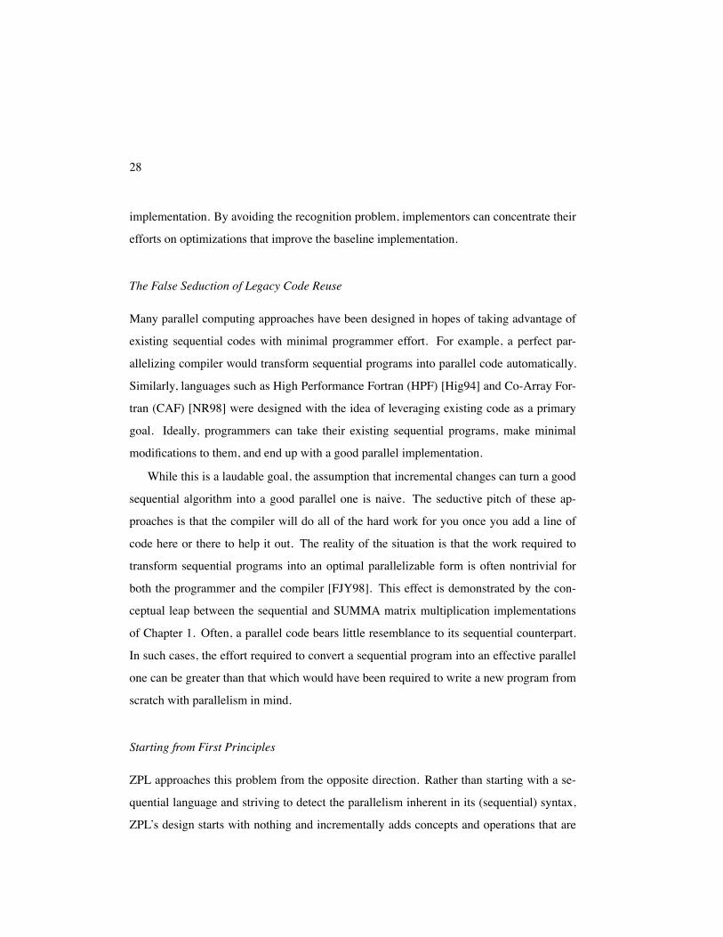
Listing 2.1: Simple Type, Constant, and Variable Declarations in ZPLtype
age = shortint;coord = record
x: integer;y: integer;
end;
constantpi: double = 3.14159265;tabsize: integer = 1000;maxage: age = 128;
var done: boolean;length: integer;name: string;origin: coord;table: array [1..tabsize] of complex;
implicitly parallel. By starting from first principles in this way, ZPL was able to avoid
supporting language constructs that disable parallelism. As an example, ZPL does not per-
mit traditional scalar indexing of its parallel arrays, due to the fact that it is an inherently
sequential construct. This approach forces programmers to consider the opportunities for
parallelism in a program from its inception, rather than doing the minimal amount of work
to get the compiler to accept their sequential code, and then spending hours with feedback
tools trying to determine why it is not achieving good parallel performance.
ZPL’s syntax is based on Modula-2 [Wir83] rather than a more popular language like
C or Fortran. This decision reinforces the idea of “starting from scratch” by forcing C and
Fortran users to confront the notion that certain features of those languages are not present
in ZPL due to their interference with parallelism (e.g., pointers, scalar array indexing, and
common blocks). It also reinforces the idea that programmers should consider their se-
quential algorithms afresh when implementing them in parallel by making it difficult for
existing C and Fortran codes to be tweaked slightly and run through the compiler.
30
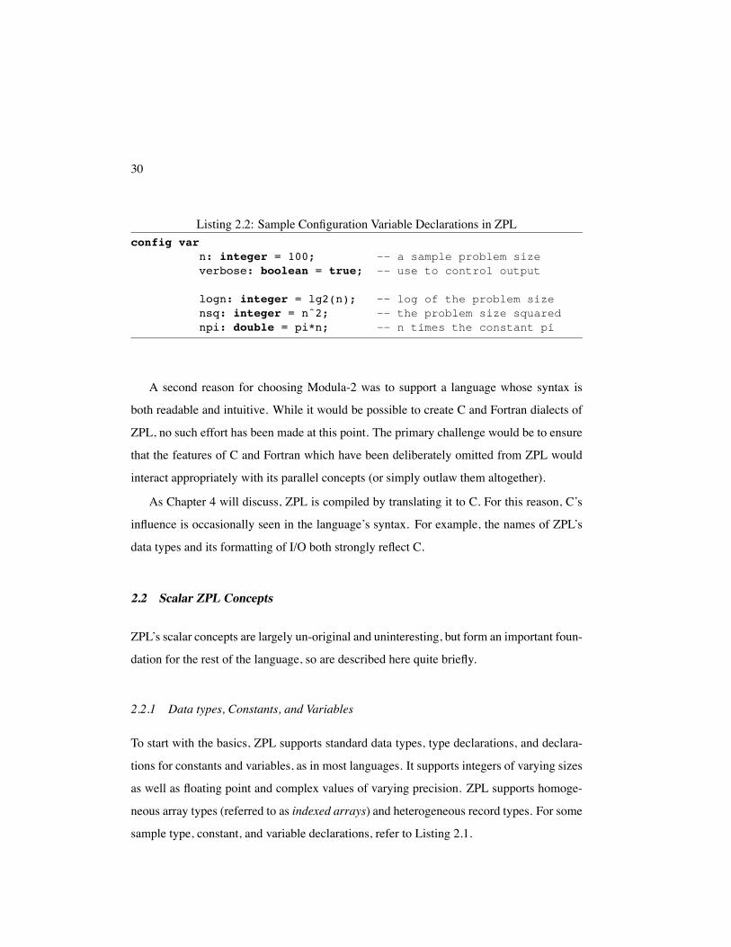
Listing 2.2: Sample Configuration Variable Declarations in ZPLconfig var
n: integer = 100; -- a sample problem sizeverbose: boolean = true; -- use to control output
logn: integer = lg2(n); -- log of the problem sizensq: integer = nˆ2; -- the problem size squarednpi: double = pi*n; -- n times the constant pi
A second reason for choosing Modula-2 was to support a language whose syntax is
both readable and intuitive. While it would be possible to create C and Fortran dialects of
ZPL, no such effort has been made at this point. The primary challenge would be to ensure
that the features of C and Fortran which have been deliberately omitted from ZPL would
interact appropriately with its parallel concepts (or simply outlaw them altogether).
As Chapter 4 will discuss, ZPL is compiled by translating it to C. For this reason, C’s
influence is occasionally seen in the language’s syntax. For example, the names of ZPL’s
data types and its formatting of I/O both strongly reflect C.
2.2 Scalar ZPL Concepts
ZPL’s scalar concepts are largely un-original and uninteresting, but form an important foun-
dation for the rest of the language, so are described here quite briefly.
2.2.1 Data types, Constants, and Variables
To start with the basics, ZPL supports standard data types, type declarations, and declara-
tions for constants and variables, as in most languages. It supports integers of varying sizes
as well as floating point and complex values of varying precision. ZPL supports homoge-
neous array types (referred to as indexed arrays) and heterogeneous record types. For some
sample type, constant, and variable declarations, refer to Listing 2.1.
31
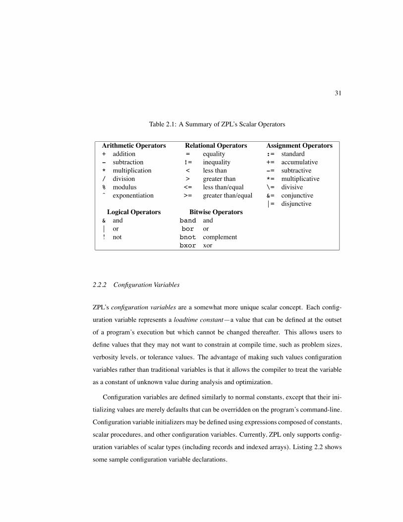
Table 2.1: A Summary of ZPL’s Scalar Operators
Arithmetic Operators+ addition- subtraction* multiplication/ division% modulusˆ exponentiation
Logical Operators& and| or! not
Relational Operators= equality!= inequality< less than> greater than<= less than/equal>= greater than/equal
Bitwise Operatorsband andbor orbnot complementbxor xor
Assignment Operators:= standard+= accumulative-= subtractive*= multiplicative\= divisive&= conjunctive|= disjunctive
2.2.2 Configuration Variables
ZPL’s configuration variables are a somewhat more unique scalar concept. Each config-
uration variable represents a loadtime constant—a value that can be defined at the outset
of a program’s execution but which cannot be changed thereafter. This allows users to
define values that they may not want to constrain at compile time, such as problem sizes,
verbosity levels, or tolerance values. The advantage of making such values configuration
variables rather than traditional variables is that it allows the compiler to treat the variable
as a constant of unknown value during analysis and optimization.
Configuration variables are defined similarly to normal constants, except that their ini-
tializing values are merely defaults that can be overridden on the program’s command-line.
Configuration variable initializers may be defined using expressions composed of constants,
scalar procedures, and other configuration variables. Currently, ZPL only supports config-
uration variables of scalar types (including records and indexed arrays). Listing 2.2 shows
some sample configuration variable declarations.
32
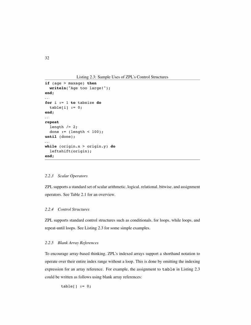
Listing 2.3: Sample Uses of ZPL’s Control Structuresif (age > maxage) thenwriteln("Age too large!");
end;
for i := 1 to tabsize dotable[i] := 0;
end;
repeatlength /= 2;done := (length < 100);
until (done);
while (origin.x > origin.y) doleftshift(origin);
end;
2.2.3 Scalar Operators
ZPL supports a standard set of scalar arithmetic, logical, relational, bitwise, and assignment
operators. See Table 2.1 for an overview.
2.2.4 Control Structures
ZPL supports standard control structures such as conditionals, for loops, while loops, and
repeat-until loops. See Listing 2.3 for some simple examples.
2.2.5 Blank Array References
To encourage array-based thinking, ZPL’s indexed arrays support a shorthand notation to
operate over their entire index range without a loop. This is done by omitting the indexing
expression for an array reference. For example, the assignment to table in Listing 2.3
could be written as follows using blank array references:
table[] := 0;
33
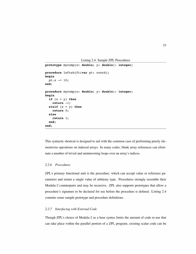
Listing 2.4: Sample ZPL Proceduresprototype mycomp(x: double; y: double): integer;
procedure leftshift(var pt: coord);beginpt.x -= 10;
end;
procedure mycomp(x: double; y: double): integer;beginif (x < y) thenreturn -1;
elsif (x = y) thenreturn 0;
elsereturn 1;
end;end;
This syntactic shortcut is designed to aid with the common case of performing purely ele-
mentwise operations on indexed arrays. In many codes, blank array references can elimi-
nate a number of trivial and uninteresting loops over an array’s indices.
2.2.6 Procedures
ZPL’s primary functional unit is the procedure, which can accept value or reference pa-
rameters and return a single value of arbitrary type. Procedures strongly resemble their
Modula-2 counterparts and may be recursive. ZPL also supports prototypes that allow a
procedure’s signature to be declared for use before the procedure is defined. Listing 2.4
contains some sample prototype and procedure definitions.
2.2.7 Interfacing with External Code
Though ZPL’s choice of Modula-2 as a base syntax limits the amount of code re-use that
can take place within the parallel portion of a ZPL program, existing scalar code can be
34
Listing 2.5: An Example of Using extern in ZPLextern constant M_PI: double;extern var errno: integer;
extern type timezone = opaque;timeval = record
tv_sec: longint;tv_usec: longint;
end;
extern prototype gettimeofday(var tv: timeval; var tz: timezone);
integrated into a ZPL program if it can be called by and linked into a C program. This is
achieved using the extern keyword which can be applied to types, constants, variables,
and procedures. External types may be partially specified or omitted completely using the
opaque keyword, which allows the programmer to store variables of external types and
pass them around, but not to operate on them directly or modify them. See Listing 2.5 for
some sample external declarations.
2.3 Regions and Parallel Arrays
As mentioned in the introduction, ZPL’s fundamental concept is that of the region. A region
is simply an index set—a set of indices in a coordinate space of arbitrary dimensions. ZPL’s
regions are regular and rectilinear in nature. In this sense they are much like traditional
arrays with no associated data. This similarity is emphasized syntactically: simple regions
are defined using syntax that resembles a traditional array’s bounds. For example, the
following shows a simple two-dimensional region and the set of indices that it describes:
[1..m, 1..n]
Regions may contain singleton dimensions which describe only a single index value. These
are defined by replacing the degenerate range with a single index (e.g., [1, 1..n] rather
than [1..1, 1..n]).
35
(a) (b) (c)
BigR
TopRow
R
CB
A
[R] A := B + C;
A CB
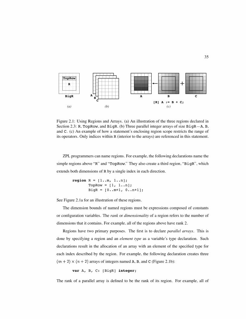
Figure 2.1: Using Regions and Arrays. (a) An illustration of the three regions declared inSection 2.3: R, TopRow, and BigR. (b) Three parallel integer arrays of size BigR—A, B,and C. (c) An example of how a statement’s enclosing region scope restricts the range ofits operators. Only indices within R (interior to the arrays) are referenced in this statement.
ZPL programmers can name regions. For example, the following declarations name the
simple regions above “R” and “TopRow.” They also create a third region, “BigR”, which
extends both dimensions of R by a single index in each direction.
region R = [1..m, 1..n];TopRow = [1, 1..n];BigR = [0..m+1, 0..n+1];
See Figure 2.1a for an illustration of these regions.
The dimension bounds of named regions must be expressions composed of constants
or configuration variables. The rank or dimensionality of a region refers to the number of
dimensions that it contains. For example, all of the regions above have rank 2.
Regions have two primary purposes. The first is to declare parallel arrays. This is
done by specifying a region and an element type as a variable’s type declaration. Such
declarations result in the allocation of an array with an element of the specified type for
each index described by the region. For example, the following declaration creates three
arrays of integers named A, B, and C (Figure 2.1b):
var A, B, C: [BigR] integer;
The rank of a parallel array is defined to be the rank of its region. For example, all of
36
the parallel arrays above have a rank of 2. Parallel arrays may not be nested. That is, the
element type of a parallel array may not contain a parallel array itself.
Parallel arrays are the primary data structure in ZPL, and will generally be referred to
as “arrays” within this dissertation. The traditional scalar arrays described in Section 2.2
will always be referred to as “indexed arrays” to avoid confusion. Note that this chapter
does not explain why parallel arrays are so named, but merely uses the term as a label. The
following chapter provides the justification for the name (though discerning readers will
possibly figure it out on their own).
The second purpose of regions is to provide indices for array references within a ZPL
statement. Unlike indexed arrays, ZPL’s parallel array elements cannot be referenced using
traditional indexing mechanisms. Instead, regions are required to specify the indices for an
array reference. As an example, consider the following statement:
[R] A := B + C;
This statement says to add arrays B and C elementwise, assigning their resulting sums to
the corresponding values in A. The statement is prefixed by the region scope “[R]” which
specifies that the addition and assignment operations should be performed for all indices
described by R—namely, the interior elements. Thus, this statement describes the
matrix addition computation from Chapter 1. Region scopes serve as a form of universal
quantification. For example, the statement above is equivalent to:
R
See Figure 2.1c for an illustration.
Using region scopes, any of ZPL’s standard scalar operators can be applied to arrays
in an elementwise manner. The chief constraint is that arrays cannot be read or written at
indices that were not in their defining region (since no data is allocated for those indices).
Region definitions may also be specified explicitly within a region scope. These are
called dynamic regions, since their bounds are typically based on expressions whose values
37
are not known until runtime. For example, the following code fragment adds row i of
arrays B and C, where i may be computed during the program’s execution.
[i, 1..n] A := B + C;
Note that technically, this region scope should contain another set of square brackets to be
consistent with the region specification syntax described previously. However, ZPL allows
programmers to drop the redundant square brackets for readability.
Subsequent sections will describe regions in more depth, but for now this example-
based overview of the ZPL language continues.
2.4 Array Operators
If ZPL could only express elementwise computations on its arrays, it would not be a very
useful language. More general computations are supported by using array operators to
modify a region scope’s indices for a given array variable or expression. This section
provides a brief introduction to the most important array operators: the @ operator, floods,
reductions, and remaps.
2.4.1 The @ Operator
The @ operator (@) is ZPL’s simplest array operator, providing a means for translating array
references using constant offset vectors known as directions. Directions are specified and
named in ZPL as follows:
direction north = [-1, 0];south = [ 1, 0];east = [ 0, 1];west = [ 0,-1];
These declarations create four vectors, one for each of the cardinal directions (Figure 2.2a).
The @ operator is applied to an array reference in a postfix manner, taking a direction
as its second operand. Applying the @ operator to an array causes the indices of the en-
closing region scope to be translated by the direction vector as they are applied to the array
38
(b)(a) (c)
A BA B C
[R] A := B@west + C@east;
east west
southnorth
[BigR] A := B@^east;
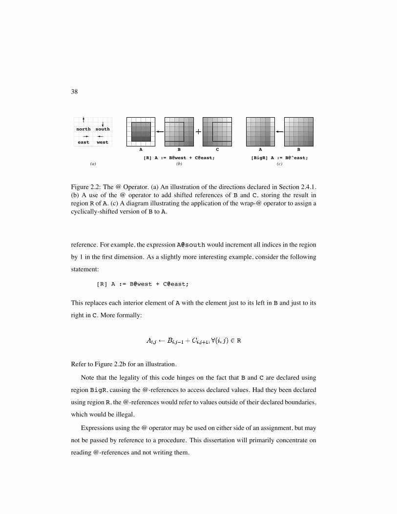
Figure 2.2: The @ Operator. (a) An illustration of the directions declared in Section 2.4.1.(b) A use of the @ operator to add shifted references of B and C, storing the result inregion R of A. (c) A diagram illustrating the application of the wrap-@ operator to assign acyclically-shifted version of B to A.
reference. For example, the expression A@south would increment all indices in the region
by 1 in the first dimension. As a slightly more interesting example, consider the following
statement:
[R] A := B@west + C@east;
This replaces each interior element of A with the element just to its left in B and just to its
right in C. More formally:
R
Refer to Figure 2.2b for an illustration.
Note that the legality of this code hinges on the fact that B and C are declared using
region BigR, causing the @-references to access declared values. Had they been declared
using region R, the @-references would refer to values outside of their declared boundaries,
which would be illegal.
Expressions using the @ operator may be used on either side of an assignment, but may
not be passed by reference to a procedure. This dissertation will primarily concentrate on
reading @-references and not writing them.
39
(b)(a)
A
(c)[TopRow] A := +<<[R] B;[R] A := >>[TopRow] B;
A B B B
[R] biggest := max<< B
biggest
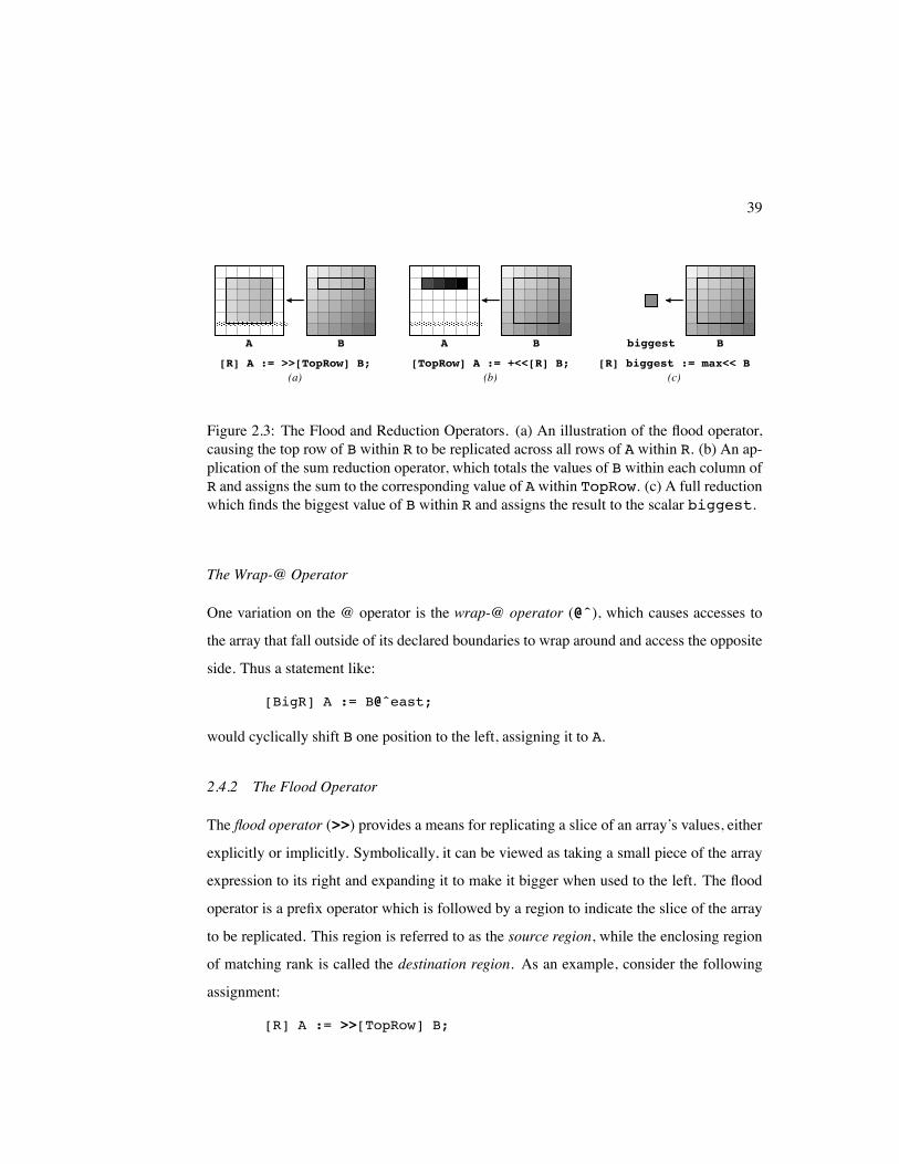
Figure 2.3: The Flood and Reduction Operators. (a) An illustration of the flood operator,causing the top row of B within R to be replicated across all rows of A within R. (b) An ap-plication of the sum reduction operator, which totals the values of B within each column ofR and assigns the sum to the corresponding value of A within TopRow. (c) A full reductionwhich finds the biggest value of B within R and assigns the result to the scalar biggest.
The Wrap-@ Operator
One variation on the @ operator is the wrap-@ operator (@ˆ), which causes accesses to
the array that fall outside of its declared boundaries to wrap around and access the opposite
side. Thus a statement like:
[BigR] A := B@ˆeast;
would cyclically shift B one position to the left, assigning it to A.
2.4.2 The Flood Operator
The flood operator (>>) provides a means for replicating a slice of an array’s values, either
explicitly or implicitly. Symbolically, it can be viewed as taking a small piece of the array
expression to its right and expanding it to make it bigger when used to the left. The flood
operator is a prefix operator which is followed by a region to indicate the slice of the array
to be replicated. This region is referred to as the source region, while the enclosing region
of matching rank is called the destination region. As an example, consider the following
assignment:
[R] A := >>[TopRow] B;
40
This statement assigns the first row of B (restricted to columns 1 through n) to rows
1 through m of A. See Figure 2.3a for an illustration.
In this statement, the flood operator’s role is to replicate the values of B described by the
source region (TopRow or [1, 1..n]) such that they conform to the destination region
(R). This action can be interpreted in either an active or a passive way. Actively, the flood
operator is taking the row of values described by TopRow and using it to create an array
of size R for assignment to A. Passively, the operator can be thought of as causing the first
dimension of indices in R to be ignored when accessing B, replacing them by the index 1.
Formally, this statement can be interpreted as follows:
R
The main legality issues for the flood operator concern the conformability of the source
and destination regions. First, they must be the same rank. In addition, each dimension
of the source region must either be a singleton (as in this example’s first dimension), or it
must be identical to the destination region (as in the second dimension). The former case
results in replication of the values described by the singleton index. The second results in a
traditional array reference.
2.4.3 The Reduction Operator
The reduction operator (<<) is the dual of the flood operator. It compresses an array’s
values down to form a smaller array. As with the flood operator, it uses prefix notation and
expects a source region to describe the values that should be reduced. The resulting size of
the expression is described by the enclosing region scope of matching rank.
Because multiple values are being collapsed into a single item, some sort of reduction
operation must also be specified to indicate how this collapsing should take place. These
operations are typically commutative and associative, and they precede the reduction oper-
ator syntactically. Built-in reduction operations include addition, multiplication, min, and
41
max, as well as logical and bitwise operators. Users may also create custom reduction
operations using scalar ZPL procedures.
As a simple example, consider the following statement which uses a plus reduction:
[TopRow] A := +<<[R] B;
This statement computes the sum of each column of B (for the rows and columns specified
by R), storing each result in the first row of the corresponding column of A. See Figure 2.3b
for an illustration. Again, this operator has both an active and a passive interpretation.
Actively, it compresses B from rows 1 through m down to a single row (the first). Passively,
it expands the reference to row 1 of B so that it refers to rows 1 through m, as combined
using addition. Formally:
TopRow R such that
The legality rules for reductions are similar to those for the flood operator. The source
and destination regions must have the same rank. In addition, each dimension of the source
and destination regions must either be the same (causing the dimension to be read nor-
mally), or the destination dimension must contain a singleton (causing the values in that
dimension to be reduced).
Full Reductions
One special case for reductions collapses an entire array to a single scalar value. This is
known as a full or complete reduction, in contrast with the partial reductions described
previously. Full reductions require only a single covering region since the scalar reference
requires no indices. A simple example is shown here:
var biggest:integer;
[R] biggest := max<< B;
This statement finds the maximum value of B within the indices described by R and assigns
it to the scalar value biggest. See Figure 2.3c for an illustration. Note that full reductions
42
A A B C
[R] A := A#[B,C];
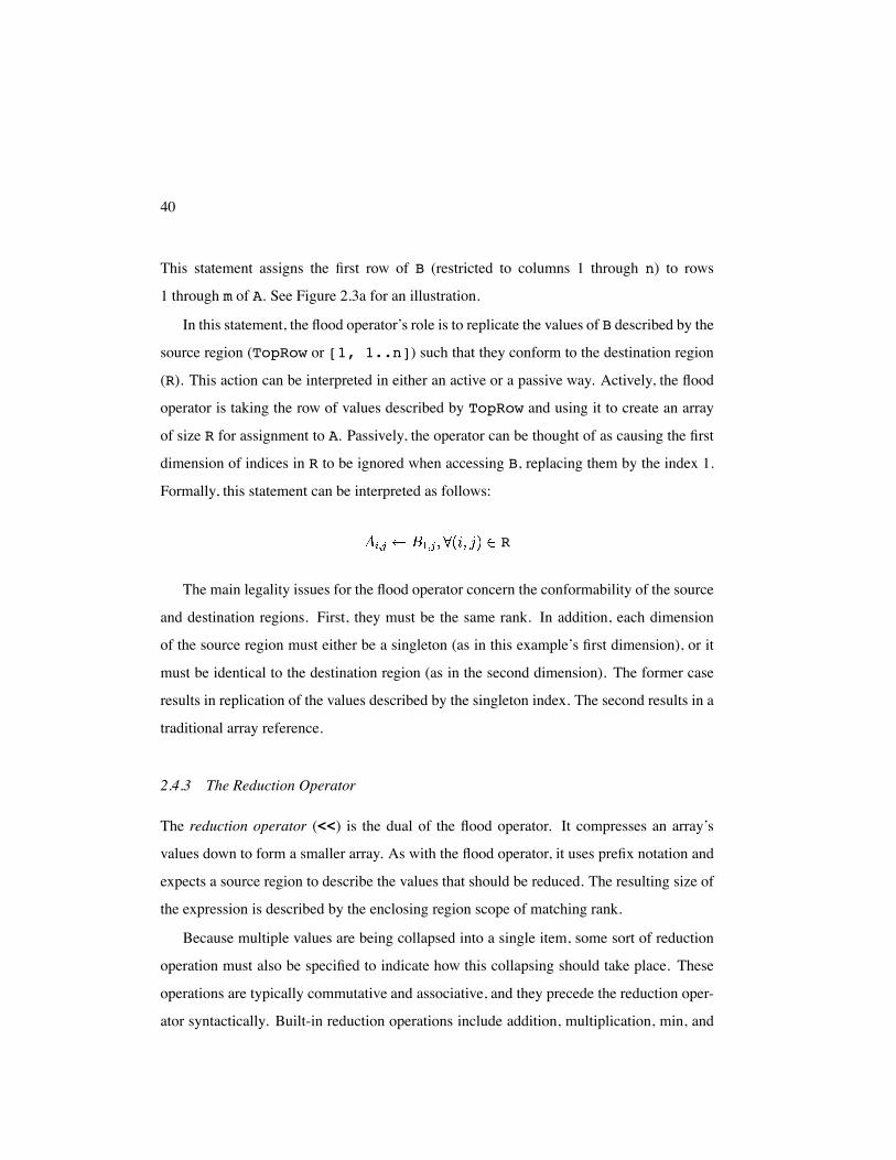
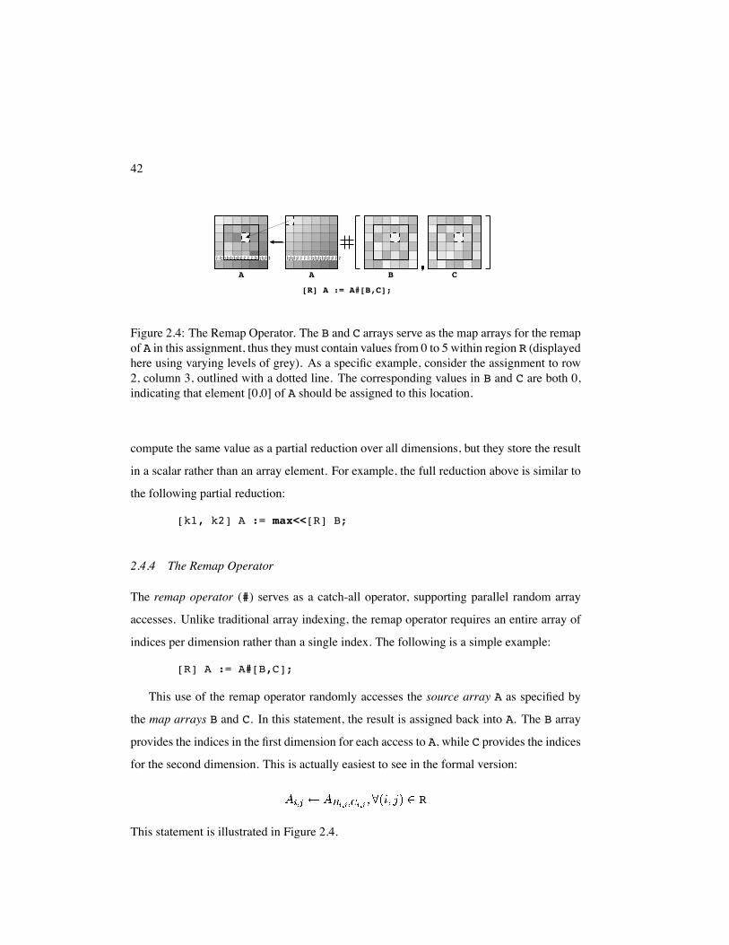
Figure 2.4: The Remap Operator. The B and C arrays serve as the map arrays for the remapof A in this assignment, thus they must contain values from 0 to 5 within region R (displayedhere using varying levels of grey). As a specific example, consider the assignment to row2, column 3, outlined with a dotted line. The corresponding values in B and C are both 0,indicating that element [0,0] of A should be assigned to this location.
compute the same value as a partial reduction over all dimensions, but they store the result
in a scalar rather than an array element. For example, the full reduction above is similar to
the following partial reduction:
[k1, k2] A := max<<[R] B;
2.4.4 The Remap Operator
The remap operator (#) serves as a catch-all operator, supporting parallel random array
accesses. Unlike traditional array indexing, the remap operator requires an entire array of
indices per dimension rather than a single index. The following is a simple example:
[R] A := A#[B,C];
This use of the remap operator randomly accesses the source array A as specified by
the map arrays B and C. In this statement, the result is assigned back into A. The B array
provides the indices in the first dimension for each access to A, while C provides the indices
for the second dimension. This is actually easiest to see in the formal version:
R
This statement is illustrated in Figure 2.4.
43
The main legality constraint for the remap operator is that the number of map arrays
must be equal to the rank of the source array so that each of its dimensions has an index. In
addition, the map arrays must not refer to indices that are outside of the source array’s defin-
ing region, since that would refer to values with no allocated storage. As Section 2.15.2 will
demonstrate, remap operators can be used to operate on arrays of different ranks (and are in
fact ZPL’s only mechanism for doing so). Remap operators may be applied to expressions
on either side of an assignment, though this dissertation focuses on uses on the right-hand
side.
2.4.5 Other Array Operators
ZPL has a few other array operators that will not be described in this thesis, most notably
the scan operator for performing parallel prefix operations, and the wrap and reflect oper-
ators for supporting boundary conditions. These are omitted in this discussion for brevity
and because they do not pose significant challenges or intrigues in ZPL’s design and im-
plementation beyond the array operators described here. For more information on these
operators, please refer to the literature [Sny99].
2.5 Formal Region Definition
Given the intuitive definitions of array operators, we now reconsider regions more for-
mally. Each dimension of a region can be represented by a 4-tuple sequence descriptor,
. The variables and represent the low and high bounds of the sequence.
The value represents the sequence’s stride, and encodes its alignment. A sequence
descriptor, , is interpreted as defining a set of integers, , as follows:
and (2.1)
For example, the descriptor describes the set of even integers between one and
six, inclusive: .
44
A -dimensional region, , is defined as a list of sequence descriptors, , where
represents the indices of the region’s th dimension:
The index set, , defined by a region is simply the cross-product of the sets specified
by each of its sequence descriptors:
For example, the index set of the 2-dimensional region would be
defined as follows:
Recall the simple region declarations described in Section 2.3 which take the following
general form:
R = [ .. , .. , , .. ]
Such declarations correspond to the following formal region definition:
These sequence descriptors specify that each dimension contains all indices from to ,
due to the trivial values used for the stride and alignment. Note that while ZPL could
allow programmers to express regions in a sequence descriptor format, the syntax used
here allows the common case to be described in a clearer, more intuitive manner.
45
2.6 Region Operators
In addition to the simple region declarations of Section 2.3, ZPL provides a set of region
operators that allow new regions to be created relative to existing ones. These are provided
to give the user a more descriptive way of creating regions than specifying them by hand.
They also provide the only means of changing a region’s stride or alignment.
Region operators are defined using a set of prepositional operators—of, in, at, and
by—that are defined for sequence descriptors. Each of these operators modifies a sequence
descriptor using an integer value, . The operators are defined as follows:
ofif
if
if
inif
if
if
at
byif
if
if
To summarize, the of and in operators modify the sequence bounds relative to the ex-
isting bounds, leaving the stride and alignment unchanged. The of operator describes a
range adjacent to the original range, whereas in describes a range interior to the previous
range. The at operator translates the sequence bounds and alignment of a sequence. The
by operator is used to scale the stride of the sequence and possibly shift the alignment,
leaving the bounds unchanged.
46
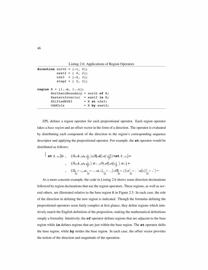
Listing 2.6: Applications of Region Operatorsdirection north = [-1, 0];
east2 = [ 0, 2];n2e3 = [-2, 3];step2 = [ 2, 2];
region R = [1..m, 1..n];NorthernBoundary = north of R;EasternInterior = east2 in R;ShiftedN2E3 = R at n2e3;OddCols = R by east2;
ZPL defines a region operator for each prepositional operator. Each region operator
takes a base region and an offset vector in the form of a direction. The operator is evaluated
by distributing each component of the direction to the region’s corresponding sequence
descriptor and applying the prepositional operator. For example, the at operator would be
distributed as follows:
at at
at at
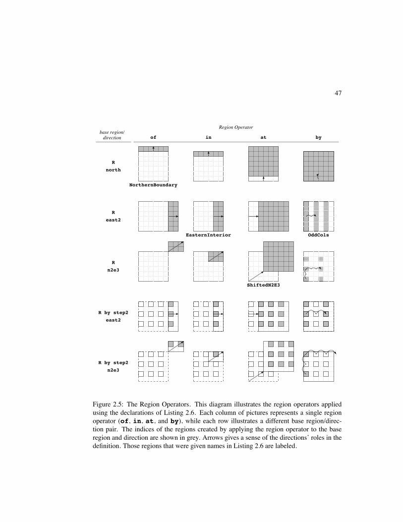
As a more concrete example, the code in Listing 2.6 shows some direction declarations
followed by region declarations that use the region operators. These regions, as well as sev-
eral others, are illustrated relative to the base region R in Figure 2.5. In each case, the role
of the direction in defining the new region is indicated. Though the formulas defining the
prepositional operators seem fairly complex at first glance, they define regions which intu-
itively match the English definition of the preposition, making the mathematical definitions
simply a formality. Intuitively, the of operator defines regions that are adjacent to the base
region while in defines regions that are just within the base region. The at operator shifts
the base region, while by strides the base region. In each case, the offset vector provides
the notion of the direction and magnitude of the operation.
47
R by step2n2e3
east2R by step2
Rnorth
Reast2
Rn2e3
base region/direction of in at by
NorthernBoundary
EasternInterior
ShiftedN2E3
OddCols
Region Operator
Figure 2.5: The Region Operators. This diagram illustrates the region operators appliedusing the declarations of Listing 2.6. Each column of pictures represents a single regionoperator (of, in, at, and by), while each row illustrates a different base region/direc-tion pair. The indices of the regions created by applying the region operator to the baseregion and direction are shown in grey. Arrows gives a sense of the directions’ roles in thedefinition. Those regions that were given names in Listing 2.6 are labeled.
48
(c)[R] A := F; [R] F := >>[1, 0..n+1] B;
(d)(b)
A F
(a)
FloodRow F
F B
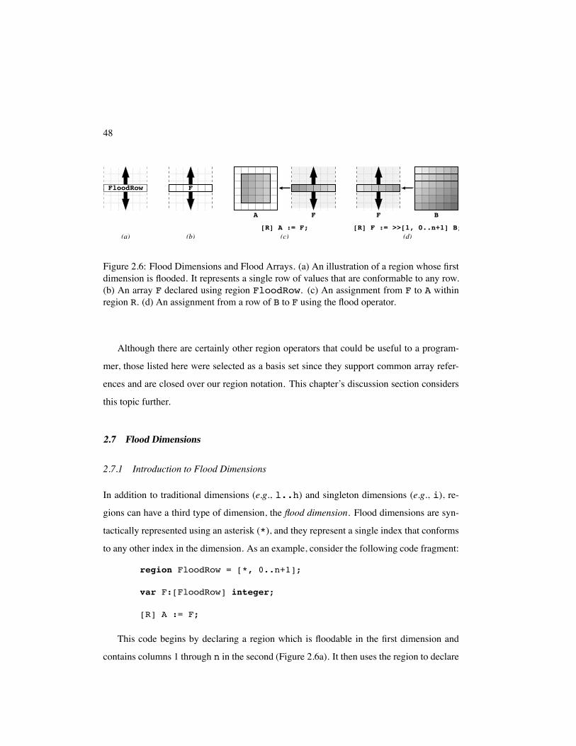
Figure 2.6: Flood Dimensions and Flood Arrays. (a) An illustration of a region whose firstdimension is flooded. It represents a single row of values that are conformable to any row.(b) An array F declared using region FloodRow. (c) An assignment from F to A withinregion R. (d) An assignment from a row of B to F using the flood operator.
Although there are certainly other region operators that could be useful to a program-
mer, those listed here were selected as a basis set since they support common array refer-
ences and are closed over our region notation. This chapter’s discussion section considers
this topic further.
2.7 Flood Dimensions
2.7.1 Introduction to Flood Dimensions
In addition to traditional dimensions (e.g., l..h) and singleton dimensions (e.g., i), re-
gions can have a third type of dimension, the flood dimension. Flood dimensions are syn-
tactically represented using an asterisk (*), and they represent a single index that conforms
to any other index in the dimension. As an example, consider the following code fragment:
region FloodRow = [*, 0..n+1];
var F:[FloodRow] integer;
[R] A := F;
This code begins by declaring a region which is floodable in the first dimension and
contains columns 1 through n in the second (Figure 2.6a). It then uses the region to declare
49
a row of integers named F (Figure 2.6b). The assignment to A reads from the appropriate
column of F for all rows in R. That is, the single row of values from F is explicitly replicated
in rows 1 through m of A. See Figure 2.6c for an illustration.
Note that FloodRow differs from a row declared using a singleton dimension like
TopRow. In particular, if F was declared using TopRow in the example above, the as-
signment would attempt to read from F in rows other than the first. This constitutes an
error since F did not allocate storage for those rows. The use of the flood dimension
in FloodRow allows it to conform to all indices, making the assignment legal.
2.7.2 Relationship with the Flood Operator
The code above illustrates a similarity between flood dimensions and the flood operator—
both are used to represent replicated values. In fact, the flood operator can be used to assign
to the values of a flood array. Consider the following example:
[FloodRow] F := >>[1, 0..n+1] B;
In this code fragment, row 1 of B is replicated by the flood operator to conform to the flood
dimension of FloodRow (Figure 2.6d). Similar assignments without the flood operator
would be illegal:
[FloodRow] F := B;[1, 0..n+1] F := B;
The first assignment is illegal because B is defined for rows 1 through m, making it am-
biguous which row of B should be stored in F. Even if B was declared to be a single row
(e.g., [1, 0..n+1]), this assignment would remain illegal since the right-hand side of
the assignment needs to conform to “all” row indices, not simply a particular one. For a
standard array like B, this can only be achieved using the flood operator. The second as-
signment is illegal because it attempts to assign to a single row of F rather than assigning
all of its rows using a flood dimension.
50
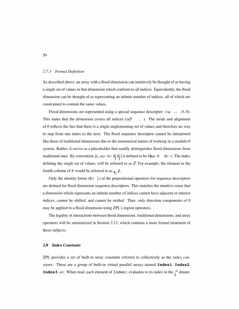
2.7.3 Formal Definition
As described above, an array with a flood dimension can intuitively be thought of as having
a single set of values in that dimension which conform to all indices. Equivalently, the flood
dimension can be thought of as representing an infinite number of indices, all of which are
constrained to contain the same values.
Flood dimensions are represented using a special sequence descriptor: ( , , 0, 0).
This states that the dimension covers all indices ( ). The stride and alignment
of 0 reflects the fact that there is a single implementing set of values and therefore no way
to step from one index to the next. The flood sequence descriptor cannot be interpreted
like those of traditional dimensions due to the nonsensical nature of working in a modulo-0
system. Rather, it serves as a placeholder that readily distinguishes flood dimensions from
traditional ones. By convention, is defined to be . The index
defining the single set of values, will be referred to as . For example, the element in the
fourth column of F would be referred to as .
Only the identity forms ( ) of the prepositional operators for sequence descriptors
are defined for flood dimension sequence descriptors. This matches the intuitive sense that
a dimension which represents an infinite number of indices cannot have adjacent or interior
indices, cannot be shifted, and cannot be strided. Thus, only direction components of 0
may be applied to a flood dimension using ZPL’s region operators.
The legality of interactions between flood dimensions, traditional dimensions, and array
operators will be summarized in Section 2.12, which contains a more formal treatment of
these subjects.
2.8 Index Constants
ZPL provides a set of built-in array constants referred to collectively as the index con-
stants. These are a group of built-in virtual parallel arrays named Index1, Index2,
Index3, etc. When read, each element of Indexi evaluates to its index in the th dimen-
51
1 n
Index2Index1Index1 Index2 A
(b)[R] A := (Index1 − 1)*n + Index2;
(a)
0
54321
0
54321
0
54321
0
54321
0
54321
0
54321
0 1 2 3 4 5
0 1 2 3 4 50 1 2 3 4 5
0 1 2 3 4 5
0 1 2 3 4 50 1 2 3 4 5
0
54321
0
54321
0
54321
0
54321
0
54321
0
54321
0 1 2 3 4 5
0 1 2 3 4 50 1 2 3 4 5
0 1 2 3 4 5
0 1 2 3 4 50 1 2 3 4 5
1 2 3 45 6 7 89 10111213141516
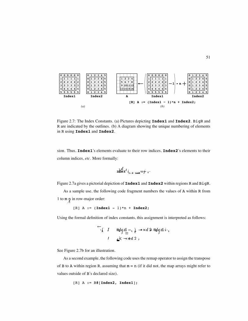
Figure 2.7: The Index Constants. (a) Pictures depicting Index1 and Index2. BigR andR are indicated by the outlines. (b) A diagram showing the unique numbering of elementsin R using Index1 and Index2.
sion. Thus, Index1’s elements evaluate to their row indices, Index2’s elements to their
column indices, etc. More formally:
i
Figure 2.7a gives a pictorial depiction of Index1 and Index2within regions R and BigR.
As a sample use, the following code fragment numbers the values of A within R from
1 to m n in row-major order:
[R] A := (Index1 - 1)*n + Index2;
Using the formal definition of index constants, this assignment is interpreted as follows:
See Figure 2.7b for an illustration.
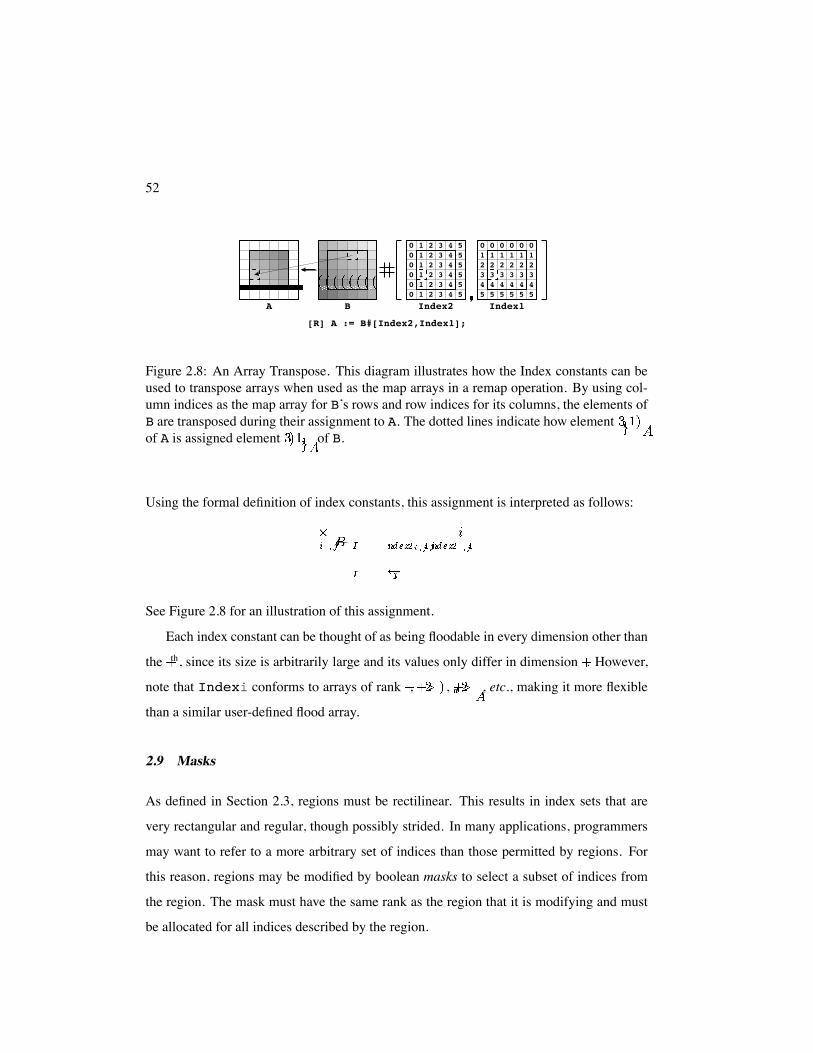
As a second example, the following code uses the remap operator to assign the transpose
of B to A within region R, assuming that m = n (if it did not, the map arrays might refer to
values outside of B’s declared size).
[R] A := B#[Index2, Index1];
52
A B Index2 Index1
[R] A := B#[Index2,Index1];
0
54321
0
54321
0
54321
0
54321
0 1 2 3 4 5
0 1 2 3 4 50 1 2 3 4 5
0 1 2 3 4 5
0 1 2 3 4 50 1 2 3 4 5
0
54321
0
54321
Figure 2.8: An Array Transpose. This diagram illustrates how the Index constants can beused to transpose arrays when used as the map arrays in a remap operation. By using col-umn indices as the map array for B’s rows and row indices for its columns, the elements ofB are transposed during their assignment to A. The dotted lines indicate how elementof A is assigned element of B.
Using the formal definition of index constants, this assignment is interpreted as follows:
See Figure 2.8 for an illustration of this assignment.
Each index constant can be thought of as being floodable in every dimension other than
the th, since its size is arbitrarily large and its values only differ in dimension . However,
note that Indexi conforms to arrays of rank , , , etc., making it more flexible
than a similar user-defined flood array.
2.9 Masks
As defined in Section 2.3, regions must be rectilinear. This results in index sets that are
very rectangular and regular, though possibly strided. In many applications, programmers
may want to refer to a more arbitrary set of indices than those permitted by regions. For
this reason, regions may be modified by boolean masks to select a subset of indices from
the region. The mask must have the same rank as the region that it is modifying and must
be allocated for all indices described by the region.
53
Mask
2 0
(a)
A
(b)[R with Mask] A := B;
BIndex1 Index2
TFT FF T F T
TFT FF T F T
0
54321
0
54321
0
54321
0
54321
0
54321
0 1 2 3 4 5
0 1 2 3 4 50 1 2 3 4 5
0 1 2 3 4 5
0 1 2 3 4 50 1 2 3 4 5
0
54321
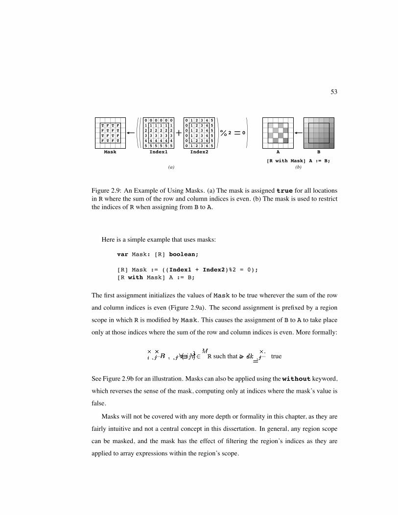
Figure 2.9: An Example of Using Masks. (a) The mask is assigned true for all locationsin R where the sum of the row and column indices is even. (b) The mask is used to restrictthe indices of R when assigning from B to A.
Here is a simple example that uses masks:
var Mask: [R] boolean;
[R] Mask := ((Index1 + Index2)%2 = 0);[R with Mask] A := B;
The first assignment initializes the values of Mask to be true wherever the sum of the row
and column indices is even (Figure 2.9a). The second assignment is prefixed by a region
scope in which R is modified by Mask. This causes the assignment of B to A to take place
only at those indices where the sum of the row and column indices is even. More formally:
R such that true
See Figure 2.9b for an illustration. Masks can also be applied using the without keyword,
which reverses the sense of the mask, computing only at indices where the mask’s value is
false.
Masks will not be covered with any more depth or formality in this chapter, as they are
fairly intuitive and not a central concept in this dissertation. In general, any region scope
can be masked, and the mask has the effect of filtering the region’s indices as they are
applied to array expressions within the region’s scope.
54
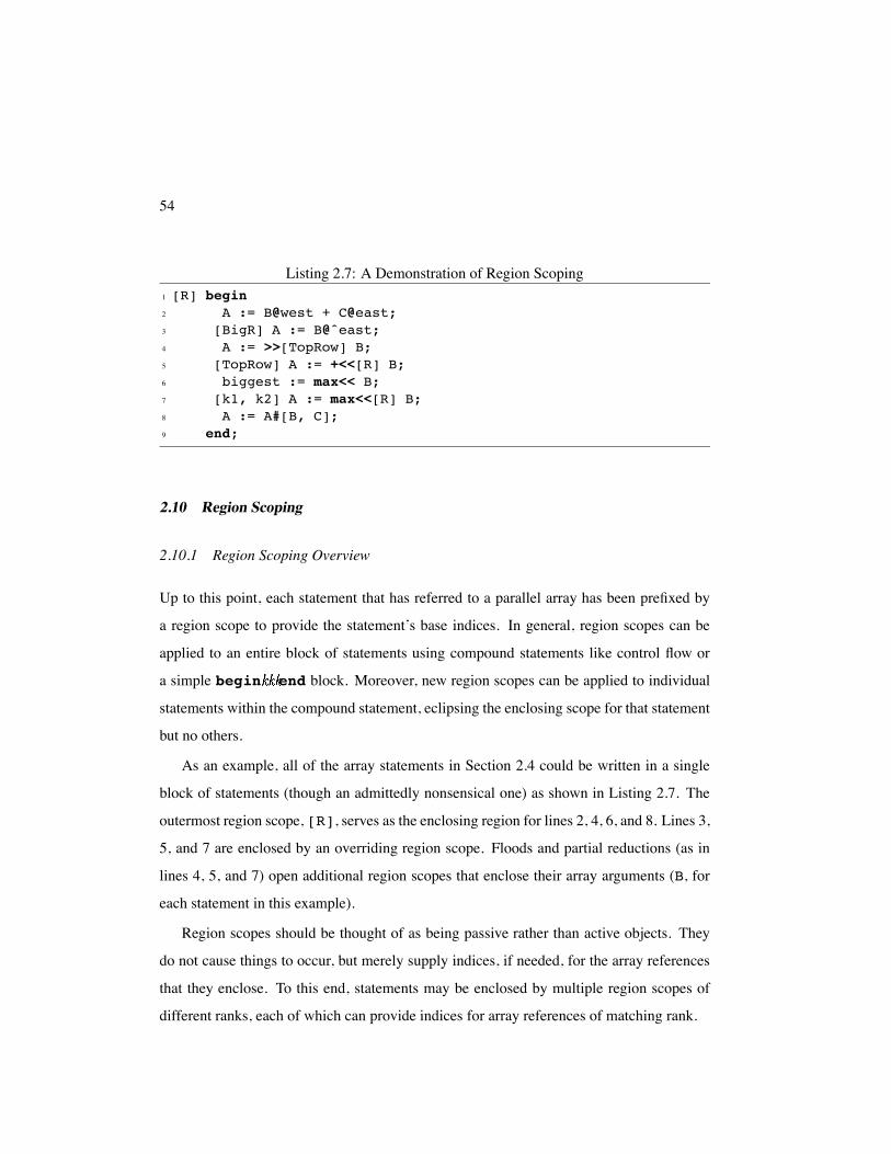
Listing 2.7: A Demonstration of Region Scoping1 [R] begin2 A := B@west + C@east;3 [BigR] A := B@ˆeast;4 A := >>[TopRow] B;5 [TopRow] A := +<<[R] B;6 biggest := max<< B;7 [k1, k2] A := max<<[R] B;8 A := A#[B, C];9 end;
2.10 Region Scoping
2.10.1 Region Scoping Overview
Up to this point, each statement that has referred to a parallel array has been prefixed by
a region scope to provide the statement’s base indices. In general, region scopes can be
applied to an entire block of statements using compound statements like control flow or
a simple begin end block. Moreover, new region scopes can be applied to individual
statements within the compound statement, eclipsing the enclosing scope for that statement
but no others.
As an example, all of the array statements in Section 2.4 could be written in a single
block of statements (though an admittedly nonsensical one) as shown in Listing 2.7. The
outermost region scope, [R], serves as the enclosing region for lines 2, 4, 6, and 8. Lines 3,
5, and 7 are enclosed by an overriding region scope. Floods and partial reductions (as in
lines 4, 5, and 7) open additional region scopes that enclose their array arguments (B, for
each statement in this example).
Region scopes should be thought of as being passive rather than active objects. They
do not cause things to occur, but merely supply indices, if needed, for the array references
that they enclose. To this end, statements may be enclosed by multiple region scopes of
different ranks, each of which can provide indices for array references of matching rank.
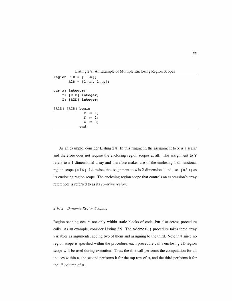
55
Listing 2.8: An Example of Multiple Enclosing Region Scopesregion R1D = [1..m];
R2D = [1..n, 1..p];
var x: integer;Y: [R1D] integer;Z: [R2D] integer;
[R1D] [R2D] beginx := 1;Y := 2;Z := 3;
end;
As an example, consider Listing 2.8. In this fragment, the assignment to x is a scalar
and therefore does not require the enclosing region scopes at all. The assignment to Y
refers to a 1-dimensional array and therefore makes use of the enclosing 1-dimensional
region scope [R1D]. Likewise, the assignment to Z is 2-dimensional and uses [R2D] as
its enclosing region scope. The enclosing region scope that controls an expression’s array
references is referred to as its covering region.
2.10.2 Dynamic Region Scoping
Region scoping occurs not only within static blocks of code, but also across procedure
calls. As an example, consider Listing 2.9. The addmat() procedure takes three array
variables as arguments, adding two of them and assigning to the third. Note that since no
region scope is specified within the procedure, each procedure call’s enclosing 2D region
scope will be used during execution. Thus, the first call performs the computation for all
indices within R, the second performs it for the top row of R, and the third performs it for
the th column of R.
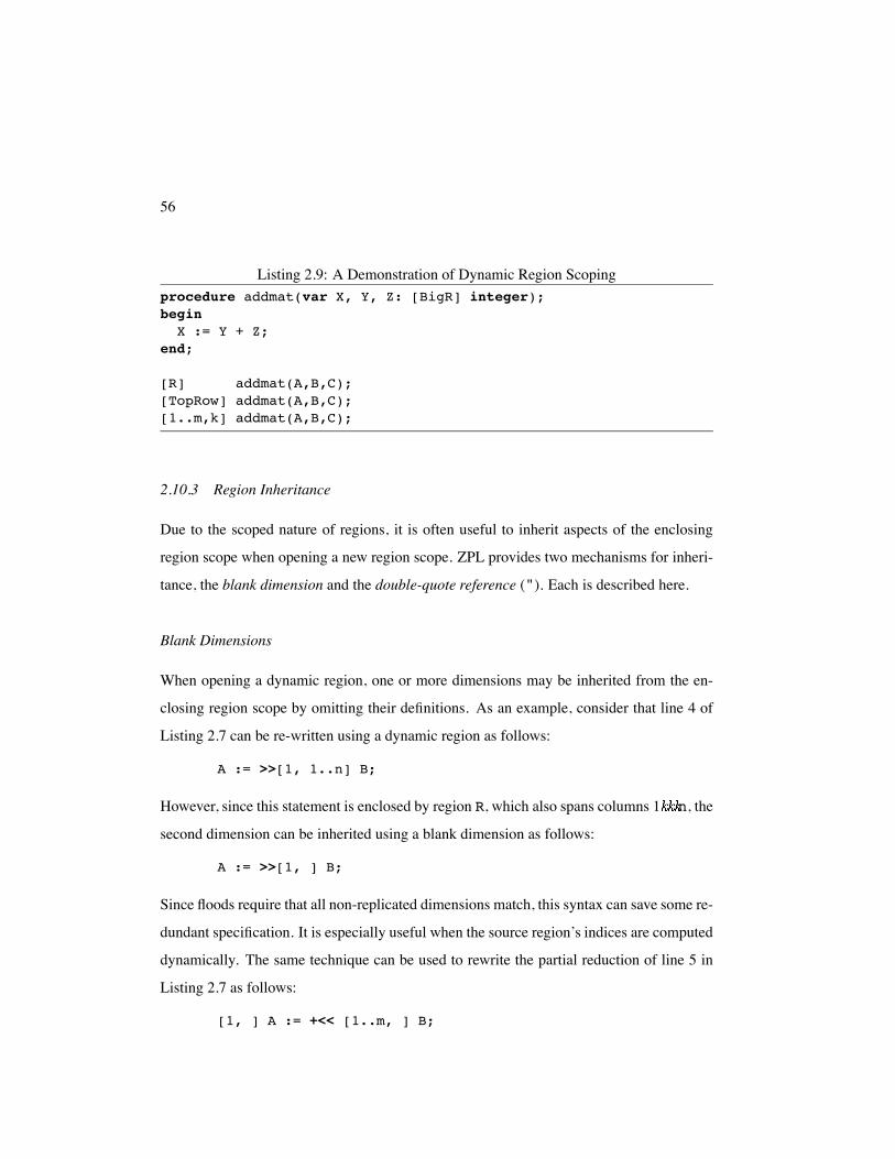
56
Listing 2.9: A Demonstration of Dynamic Region Scopingprocedure addmat(var X, Y, Z: [BigR] integer);beginX := Y + Z;
end;
[R] addmat(A,B,C);[TopRow] addmat(A,B,C);[1..m,k] addmat(A,B,C);
2.10.3 Region Inheritance
Due to the scoped nature of regions, it is often useful to inherit aspects of the enclosing
region scope when opening a new region scope. ZPL provides two mechanisms for inheri-
tance, the blank dimension and the double-quote reference ("). Each is described here.
Blank Dimensions
When opening a dynamic region, one or more dimensions may be inherited from the en-
closing region scope by omitting their definitions. As an example, consider that line 4 of
Listing 2.7 can be re-written using a dynamic region as follows:
A := >>[1, 1..n] B;
However, since this statement is enclosed by region R, which also spans columns 1 n, the
second dimension can be inherited using a blank dimension as follows:
A := >>[1, ] B;
Since floods require that all non-replicated dimensions match, this syntax can save some re-
dundant specification. It is especially useful when the source region’s indices are computed
dynamically. The same technique can be used to rewrite the partial reduction of line 5 in
Listing 2.7 as follows:
[1, ] A := +<< [1..m, ] B;
57
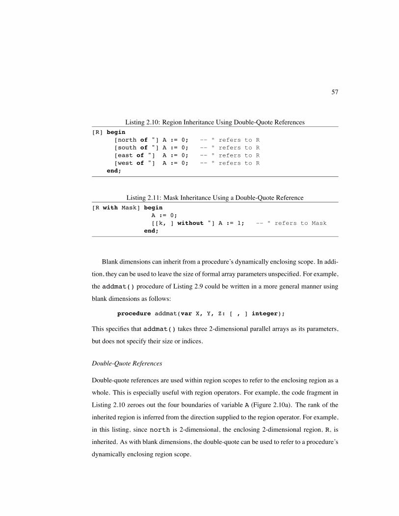
Listing 2.10: Region Inheritance Using Double-Quote References[R] begin
[north of "] A := 0; -- " refers to R[south of "] A := 0; -- " refers to R[east of "] A := 0; -- " refers to R[west of "] A := 0; -- " refers to R
end;
Listing 2.11: Mask Inheritance Using a Double-Quote Reference[R with Mask] begin
A := 0;[[k, ] without "] A := 1; -- " refers to Mask
end;
Blank dimensions can inherit from a procedure’s dynamically enclosing scope. In addi-
tion, they can be used to leave the size of formal array parameters unspecified. For example,
the addmat() procedure of Listing 2.9 could be written in a more general manner using
blank dimensions as follows:
procedure addmat(var X, Y, Z: [ , ] integer);
This specifies that addmat() takes three 2-dimensional parallel arrays as its parameters,
but does not specify their size or indices.
Double-Quote References
Double-quote references are used within region scopes to refer to the enclosing region as a
whole. This is especially useful with region operators. For example, the code fragment in
Listing 2.10 zeroes out the four boundaries of variable A (Figure 2.10a). The rank of the
inherited region is inferred from the direction supplied to the region operator. For example,
in this listing, since north is 2-dimensional, the enclosing 2-dimensional region, R, is
inherited. As with blank dimensions, the double-quote can be used to refer to a procedure’s
dynamically enclosing region scope.
58
k
A A
(a) (b)
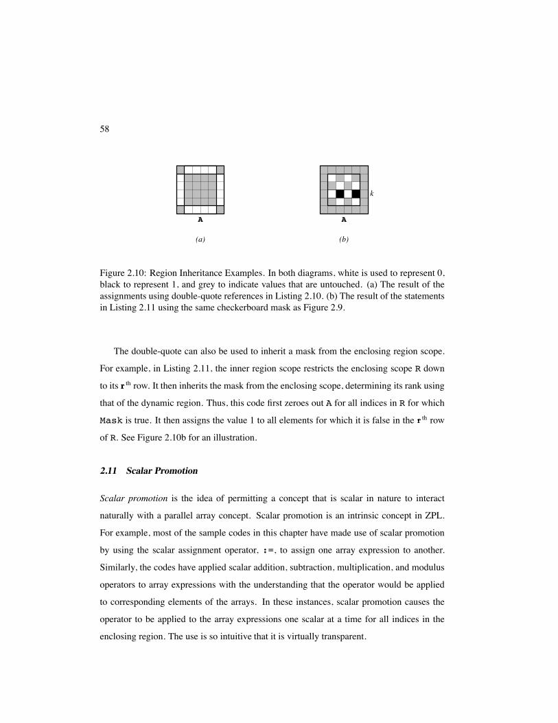
Figure 2.10: Region Inheritance Examples. In both diagrams, white is used to represent 0,black to represent 1, and grey to indicate values that are untouched. (a) The result of theassignments using double-quote references in Listing 2.10. (b) The result of the statementsin Listing 2.11 using the same checkerboard mask as Figure 2.9.
The double-quote can also be used to inherit a mask from the enclosing region scope.
For example, in Listing 2.11, the inner region scope restricts the enclosing scope R down
to its th row. It then inherits the mask from the enclosing scope, determining its rank using
that of the dynamic region. Thus, this code first zeroes out A for all indices in R for which
Mask is true. It then assigns the value 1 to all elements for which it is false in the th row
of R. See Figure 2.10b for an illustration.
2.11 Scalar Promotion
Scalar promotion is the idea of permitting a concept that is scalar in nature to interact
naturally with a parallel array concept. Scalar promotion is an intrinsic concept in ZPL.
For example, most of the sample codes in this chapter have made use of scalar promotion
by using the scalar assignment operator, :=, to assign one array expression to another.
Similarly, the codes have applied scalar addition, subtraction, multiplication, and modulus
operators to array expressions with the understanding that the operator would be applied
to corresponding elements of the arrays. In these instances, scalar promotion causes the
operator to be applied to the array expressions one scalar at a time for all indices in the
enclosing region. The use is so intuitive that it is virtually transparent.
59
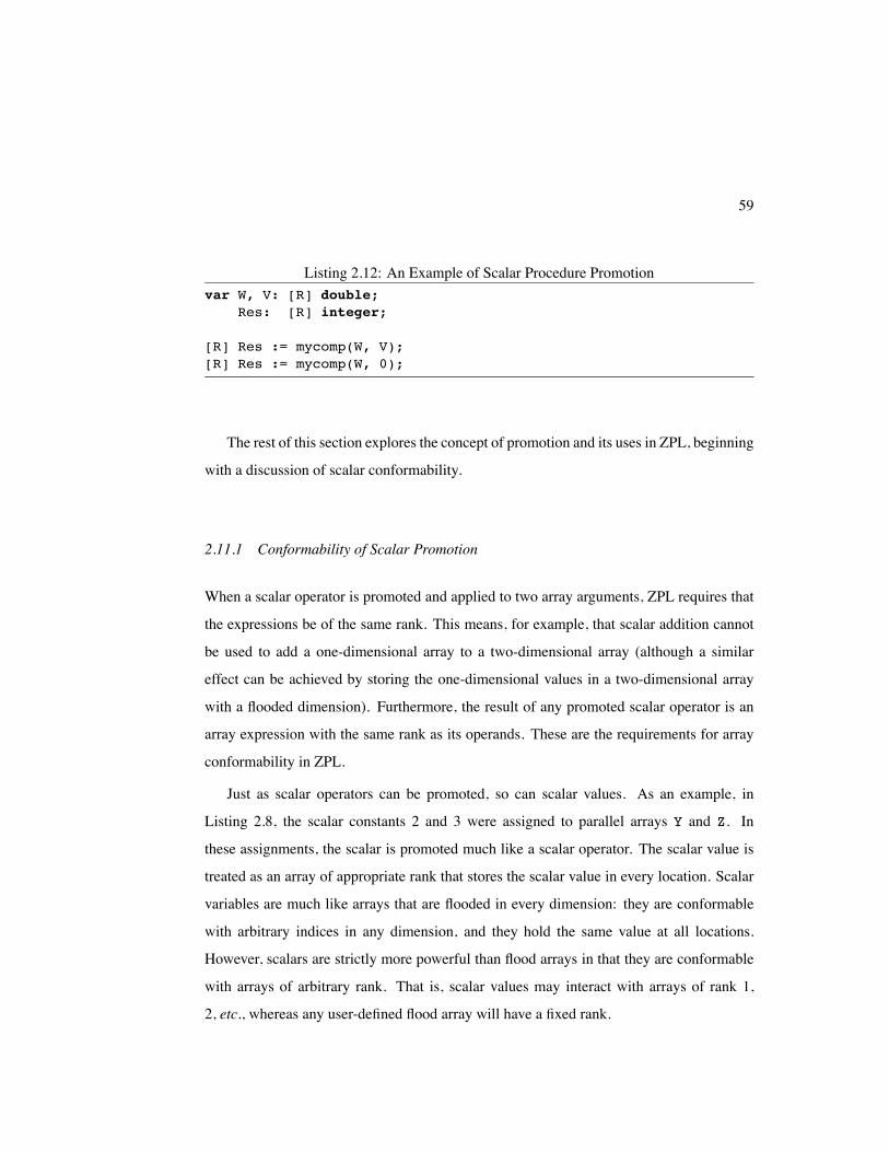
Listing 2.12: An Example of Scalar Procedure Promotionvar W, V: [R] double;
Res: [R] integer;
[R] Res := mycomp(W, V);[R] Res := mycomp(W, 0);
The rest of this section explores the concept of promotion and its uses in ZPL, beginning
with a discussion of scalar conformability.
2.11.1 Conformability of Scalar Promotion
When a scalar operator is promoted and applied to two array arguments, ZPL requires that
the expressions be of the same rank. This means, for example, that scalar addition cannot
be used to add a one-dimensional array to a two-dimensional array (although a similar
effect can be achieved by storing the one-dimensional values in a two-dimensional array
with a flooded dimension). Furthermore, the result of any promoted scalar operator is an
array expression with the same rank as its operands. These are the requirements for array
conformability in ZPL.
Just as scalar operators can be promoted, so can scalar values. As an example, in
Listing 2.8, the scalar constants 2 and 3 were assigned to parallel arrays Y and Z. In
these assignments, the scalar is promoted much like a scalar operator. The scalar value is
treated as an array of appropriate rank that stores the scalar value in every location. Scalar
variables are much like arrays that are flooded in every dimension: they are conformable
with arbitrary indices in any dimension, and they hold the same value at all locations.
However, scalars are strictly more powerful than flood arrays in that they are conformable
with arrays of arbitrary rank. That is, scalar values may interact with arrays of rank 1,
2, etc., whereas any user-defined flood array will have a fixed rank.
60
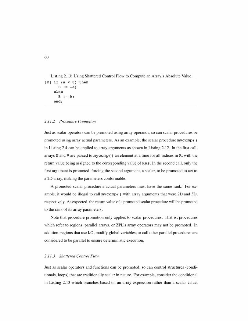
Listing 2.13: Using Shattered Control Flow to Compute an Array’s Absolute Value[R] if (A < 0) then
B := -A;elseB := A;
end;
2.11.2 Procedure Promotion
Just as scalar operators can be promoted using array operands, so can scalar procedures be
promoted using array actual parameters. As an example, the scalar procedure mycomp()
in Listing 2.4 can be applied to array arguments as shown in Listing 2.12. In the first call,
arrays W and V are passed to mycomp() an element at a time for all indices in R, with the
return value being assigned to the corresponding value of Res. In the second call, only the
first argument is promoted, forcing the second argument, a scalar, to be promoted to act as
a 2D array, making the parameters conformable.
A promoted scalar procedure’s actual parameters must have the same rank. For ex-
ample, it would be illegal to call mycomp() with array arguments that were 2D and 3D,
respectively. As expected, the return value of a promoted scalar procedure will be promoted
to the rank of its array parameters.
Note that procedure promotion only applies to scalar procedures. That is, procedures
which refer to regions, parallel arrays, or ZPL’s array operators may not be promoted. In
addition, regions that use I/O, modify global variables, or call other parallel procedures are
considered to be parallel to ensure deterministic execution.
2.11.3 Shattered Control Flow
Just as scalar operators and functions can be promoted, so can control structures (condi-
tionals, loops) that are traditionally scalar in nature. For example, consider the conditional
in Listing 2.13 which branches based on an array expression rather than a scalar value.
61
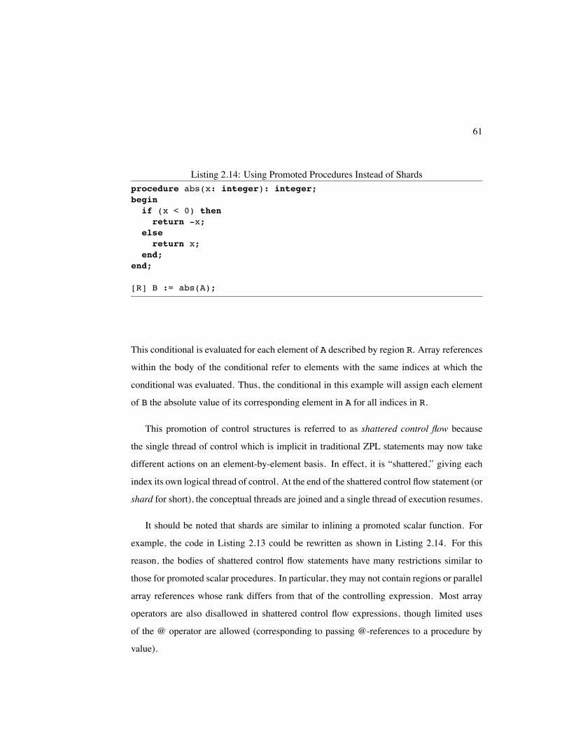
Listing 2.14: Using Promoted Procedures Instead of Shardsprocedure abs(x: integer): integer;beginif (x < 0) thenreturn -x;
elsereturn x;
end;end;
[R] B := abs(A);
This conditional is evaluated for each element of A described by region R. Array references
within the body of the conditional refer to elements with the same indices at which the
conditional was evaluated. Thus, the conditional in this example will assign each element
of B the absolute value of its corresponding element in A for all indices in R.
This promotion of control structures is referred to as shattered control flow because
the single thread of control which is implicit in traditional ZPL statements may now take
different actions on an element-by-element basis. In effect, it is “shattered,” giving each
index its own logical thread of control. At the end of the shattered control flow statement (or
shard for short), the conceptual threads are joined and a single thread of execution resumes.
It should be noted that shards are similar to inlining a promoted scalar function. For
example, the code in Listing 2.13 could be rewritten as shown in Listing 2.14. For this
reason, the bodies of shattered control flow statements have many restrictions similar to
those for promoted scalar procedures. In particular, they may not contain regions or parallel
array references whose rank differs from that of the controlling expression. Most array
operators are also disallowed in shattered control flow expressions, though limited uses
of the @ operator are allowed (corresponding to passing @-references to a procedure by
value).
62
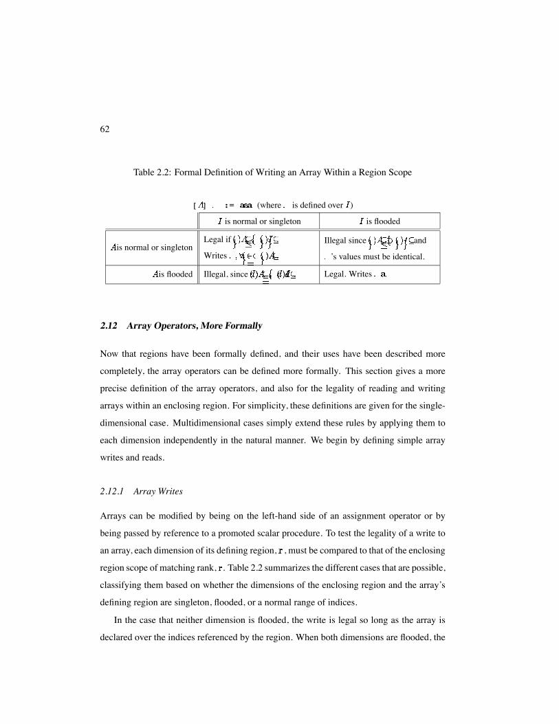
Table 2.2: Formal Definition of Writing an Array Within a Region Scope
[ ] := (where is defined over )
is normal or singleton is flooded
is normal or singletonLegal if .
Writes .
Illegal since and
’s values must be identical.
is flooded Illegal, since . Legal. Writes .
2.12 Array Operators, More Formally
Now that regions have been formally defined, and their uses have been described more
completely, the array operators can be defined more formally. This section gives a more
precise definition of the array operators, and also for the legality of reading and writing
arrays within an enclosing region. For simplicity, these definitions are given for the single-
dimensional case. Multidimensional cases simply extend these rules by applying them to
each dimension independently in the natural manner. We begin by defining simple array
writes and reads.
2.12.1 Array Writes
Arrays can be modified by being on the left-hand side of an assignment operator or by
being passed by reference to a promoted scalar procedure. To test the legality of a write to
an array, each dimension of its defining region, , must be compared to that of the enclosing
region scope of matching rank, . Table 2.2 summarizes the different cases that are possible,
classifying them based on whether the dimensions of the enclosing region and the array’s
defining region are singleton, flooded, or a normal range of indices.
In the case that neither dimension is flooded, the write is legal so long as the array is
declared over the indices referenced by the region. When both dimensions are flooded, the
63
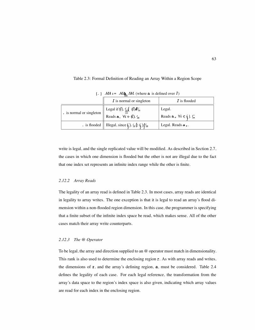
Table 2.3: Formal Definition of Reading an Array Within a Region Scope
[ ] := (where is defined over )
is normal or singleton is flooded
is normal or singletonLegal if .
Reads .
Legal.
Reads .
is flooded Illegal, since . Legal. Reads .
write is legal, and the single replicated value will be modified. As described in Section 2.7,
the cases in which one dimension is flooded but the other is not are illegal due to the fact
that one index set represents an infinite index range while the other is finite.
2.12.2 Array Reads
The legality of an array read is defined in Table 2.3. In most cases, array reads are identical
in legality to array writes. The one exception is that it is legal to read an array’s flood di-
mension within a non-flooded region dimension. In this case, the programmer is specifying
that a finite subset of the infinite index space be read, which makes sense. All of the other
cases match their array write counterparts.
2.12.3 The @ Operator
To be legal, the array and direction supplied to an @ operator must match in dimensionality.
This rank is also used to determine the enclosing region . As with array reads and writes,
the dimensions of , and the array’s defining region, , must be considered. Table 2.4
defines the legality of each case. For each legal reference, the transformation from the
array’s data space to the region’s index space is also given, indicating which array values
are read for each index in the enclosing region.
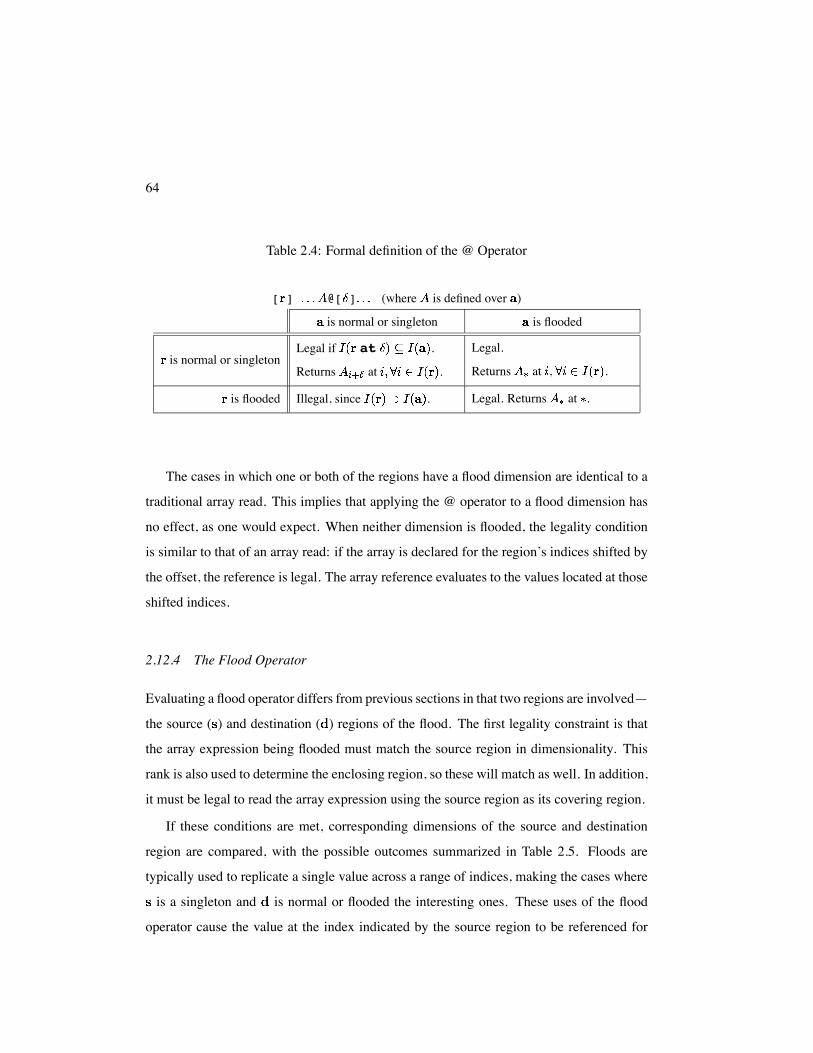
64
Table 2.4: Formal definition of the @ Operator
[ ] @[ ] (where is defined over )
is normal or singleton is flooded
is normal or singletonLegal if at .
Returns at .
Legal.
Returns at , .
is flooded Illegal, since . Legal. Returns at .
The cases in which one or both of the regions have a flood dimension are identical to a
traditional array read. This implies that applying the @ operator to a flood dimension has
no effect, as one would expect. When neither dimension is flooded, the legality condition
is similar to that of an array read: if the array is declared for the region’s indices shifted by
the offset, the reference is legal. The array reference evaluates to the values located at those
shifted indices.
2.12.4 The Flood Operator
Evaluating a flood operator differs from previous sections in that two regions are involved—
the source ( ) and destination ( ) regions of the flood. The first legality constraint is that
the array expression being flooded must match the source region in dimensionality. This
rank is also used to determine the enclosing region, so these will match as well. In addition,
it must be legal to read the array expression using the source region as its covering region.
If these conditions are met, corresponding dimensions of the source and destination
region are compared, with the possible outcomes summarized in Table 2.5. Floods are
typically used to replicate a single value across a range of indices, making the cases where
is a singleton and is normal or flooded the interesting ones. These uses of the flood
operator cause the value at the index indicated by the source region to be referenced for
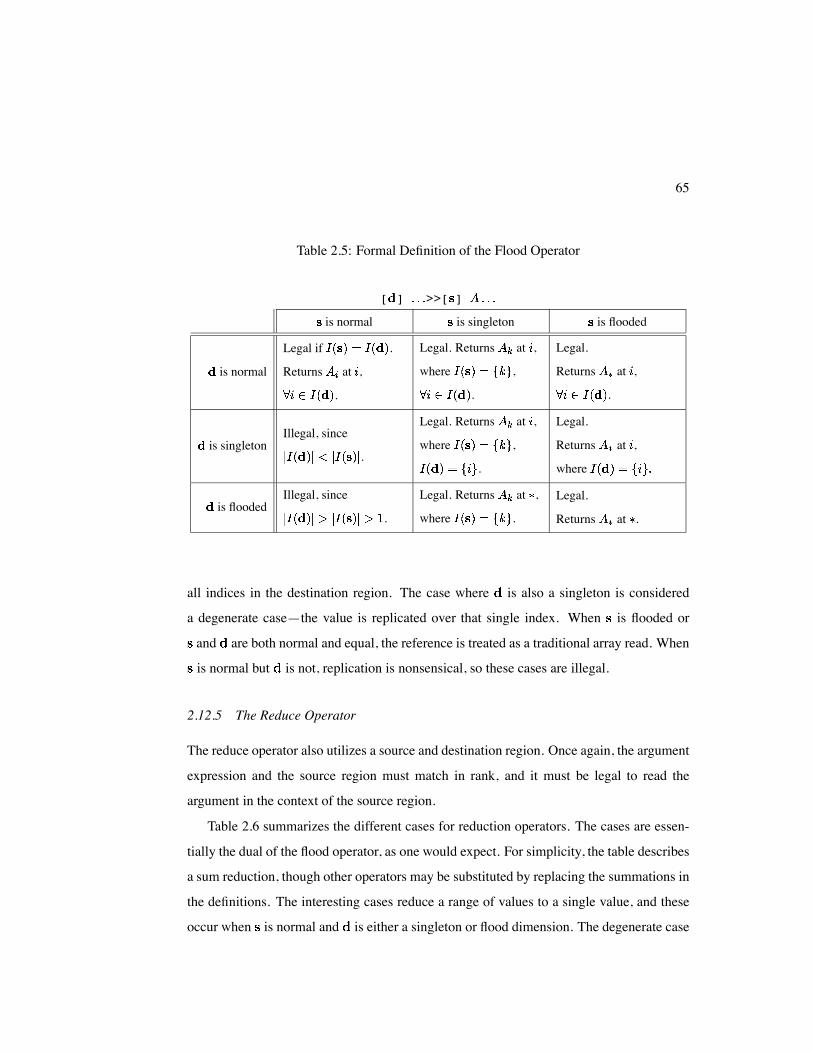
65
Table 2.5: Formal Definition of the Flood Operator
[ ] >>[ ]
is normal is singleton is flooded
is normal
Legal if .
Returns at ,
.
Legal. Returns at ,
where ,
.
Legal.
Returns at ,
.
is singletonIllegal, since
.
Legal. Returns at ,
where ,
.
Legal.
Returns at ,
where
is floodedIllegal, since
.
Legal. Returns at ,
where .
Legal.
Returns at .
all indices in the destination region. The case where is also a singleton is considered
a degenerate case—the value is replicated over that single index. When is flooded or
and are both normal and equal, the reference is treated as a traditional array read. When
is normal but is not, replication is nonsensical, so these cases are illegal.
2.12.5 The Reduce Operator
The reduce operator also utilizes a source and destination region. Once again, the argument
expression and the source region must match in rank, and it must be legal to read the
argument in the context of the source region.
Table 2.6 summarizes the different cases for reduction operators. The cases are essen-
tially the dual of the flood operator, as one would expect. For simplicity, the table describes
a sum reduction, though other operators may be substituted by replacing the summations in
the definitions. The interesting cases reduce a range of values to a single value, and these
occur when is normal and is either a singleton or flood dimension. The degenerate case
66
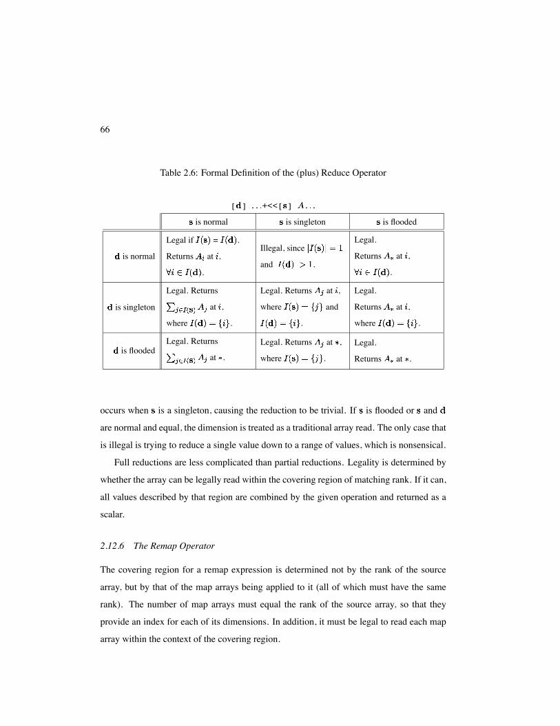
Table 2.6: Formal Definition of the (plus) Reduce Operator
[ ] +<<[ ]
is normal is singleton is flooded
is normal
Legal if = .
Returns at ,
.
Illegal, since
and .
Legal.
Returns at ,
.
is singleton
Legal. Returns
at ,
where .
Legal. Returns at ,
where and
.
Legal.
Returns at ,
where .
is floodedLegal. Returns
at .
Legal. Returns at ,
where .
Legal.
Returns at .
occurs when is a singleton, causing the reduction to be trivial. If is flooded or and
are normal and equal, the dimension is treated as a traditional array read. The only case that
is illegal is trying to reduce a single value down to a range of values, which is nonsensical.
Full reductions are less complicated than partial reductions. Legality is determined by
whether the array can be legally read within the covering region of matching rank. If it can,
all values described by that region are combined by the given operation and returned as a
scalar.
2.12.6 The Remap Operator
The covering region for a remap expression is determined not by the rank of the source
array, but by that of the map arrays being applied to it (all of which must have the same
rank). The number of map arrays must equal the rank of the source array, so that they
provide an index for each of its dimensions. In addition, it must be legal to read each map
array within the context of the covering region.
67
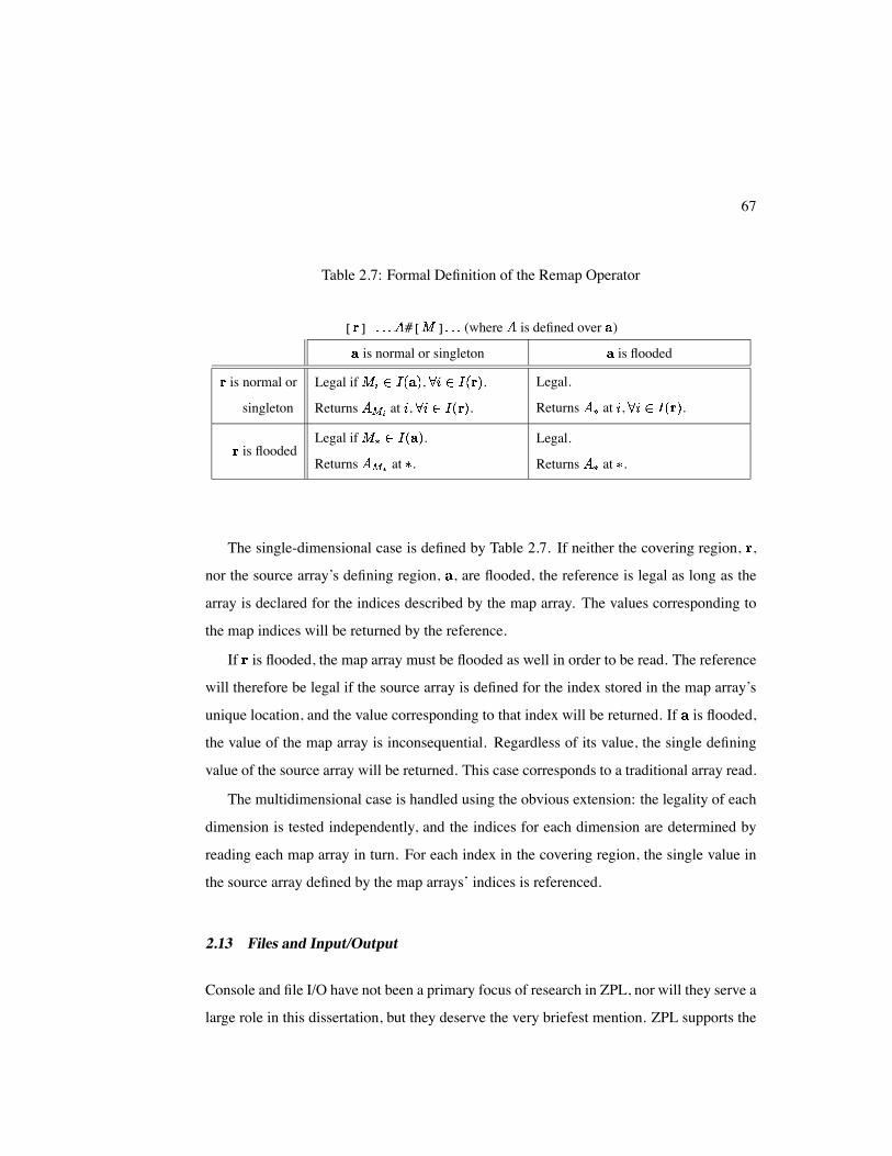
Table 2.7: Formal Definition of the Remap Operator
[ ] #[ ] (where is defined over )
is normal or singleton is flooded
is normal or
singleton
Legal if , .
Returns at , .
Legal.
Returns at , .
is floodedLegal if .
Returns at .
Legal.
Returns at .
The single-dimensional case is defined by Table 2.7. If neither the covering region, ,
nor the source array’s defining region, , are flooded, the reference is legal as long as the
array is declared for the indices described by the map array. The values corresponding to
the map indices will be returned by the reference.
If is flooded, the map array must be flooded as well in order to be read. The reference
will therefore be legal if the source array is defined for the index stored in the map array’s
unique location, and the value corresponding to that index will be returned. If is flooded,
the value of the map array is inconsequential. Regardless of its value, the single defining
value of the source array will be returned. This case corresponds to a traditional array read.
The multidimensional case is handled using the obvious extension: the legality of each
dimension is tested independently, and the indices for each dimension are determined by
reading each map array in turn. For each index in the covering region, the single value in
the source array defined by the map arrays’ indices is referenced.
2.13 Files and Input/Output
Console and file I/O have not been a primary focus of research in ZPL, nor will they serve a
large role in this dissertation, but they deserve the very briefest mention. ZPL supports the
68
ability to open files for reading and writing, and also supports the standard console input,
output, and error streams (zin, zout, and zerr, respectively). ZPL supports read(),
write(), and writeln() statements that can be used to read or write expressions to
one of these streams or to a file. Expressions can be formatted using control strings like
those accepted by C’s printf() and scanf() routines. Binary I/O is supported using
the bread() and bwrite() statements. Array expressions are read or written for all
indices in the enclosing region scope of the same rank, in row-major order (with some
minimal formatting in the case of text output).
2.14 ZPL Summary
This chapter’s description of ZPL concludes with a brief recap of its contents. To summa-
rize, ZPL contains traditional scalar language constructs using a Modula-based syntax. In
addition, ZPL supports configuration variables that serve as runtime constants and can be
set on the resulting executable’s command line.
ZPL supports array-based programming using the concept of the region to represent
a regular, rectilinear set of indices. Regions may be named or specified in-line. A re-
gion’s dimensions can represent a range of indices (potentially strided), a single index, or
a replicated index using a flood dimension. Region operators may also be used to create
new regions from existing ones. Regions are used to declare parallel arrays, which are the
primary unit of computation in ZPL. The language also supplies built-in Indexi array
constants which evaluate to their own indices in a particular dimension.
Regions are also used to define region scopes, which passively provide indices for paral-
lel array references and expressions of matching rank. Array operators are used to transform
a region’s indices as applied to a particular array expression. Array operators support trans-
lation, replication, reduction, or general remapping of an array’s values. Region scopes are
dynamically scoped and may inherit from their enclosing scopes of matching rank. Masks
can be applied to region scopes to filter out a subset of their indices.
69
ZPL allows the promotion of scalar operators, values, functions, and control flow to
interact with arrays in a natural manner. It also contains support for binary and text I/O of
scalar and array expressions to files or the console.
Nagging Questions
At this point, it is likely that there are several aspects of ZPL which seem arbitrary or
strange. For example: Why does ZPL prevent interactions between regions and arrays of
different rank if they are the same shape? Since the remap operator can be used to express
translations, floods, and reductions, why does ZPL bother supporting other array operators?
Why can ZPL regions only be applied to statements and certain array operators rather than
arbitrary expressions? Why are flood dimensions non-conformable with singleton dimen-
sions, given that they each represent a single set of defining values? Why are @-references
not allowed to be passed by reference to parallel procedures?
The answers to these questions are based on the parallel interpretation of regions and
arrays, and therefore will have to wait until the following chapter. For now, let us turn our
attention to some sample applications written in ZPL.
2.15 Sample Codes
This section contains several sample applications written in ZPL. The problems consid-
ered are the Jacobi iteration, matrix-vector multiplication, matrix multiplication, and tridi-
agonal matrix multiplication. These applications were chosen because they are simple,
well-known, and useful for demonstrating the language features described in this chap-
ter. Most of the problems have a few different implementations to illustrate different ap-
proaches in ZPL. For a larger variety of application domains in ZPL, please consult the
literature [WGS00, DLMW95, RBS96, LLST95, Sny99].
70
4
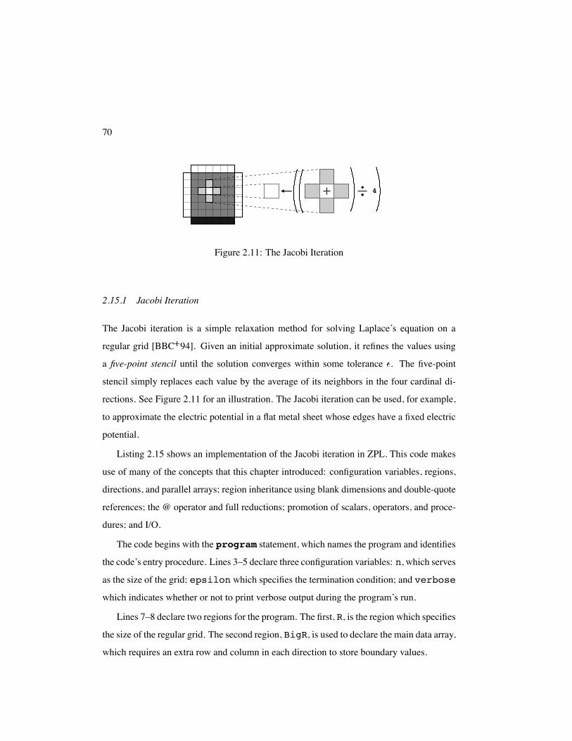
Figure 2.11: The Jacobi Iteration
2.15.1 Jacobi Iteration
The Jacobi iteration is a simple relaxation method for solving Laplace’s equation on a
regular grid [BBC 94]. Given an initial approximate solution, it refines the values using
a five-point stencil until the solution converges within some tolerance . The five-point
stencil simply replaces each value by the average of its neighbors in the four cardinal di-
rections. See Figure 2.11 for an illustration. The Jacobi iteration can be used, for example,
to approximate the electric potential in a flat metal sheet whose edges have a fixed electric
potential.
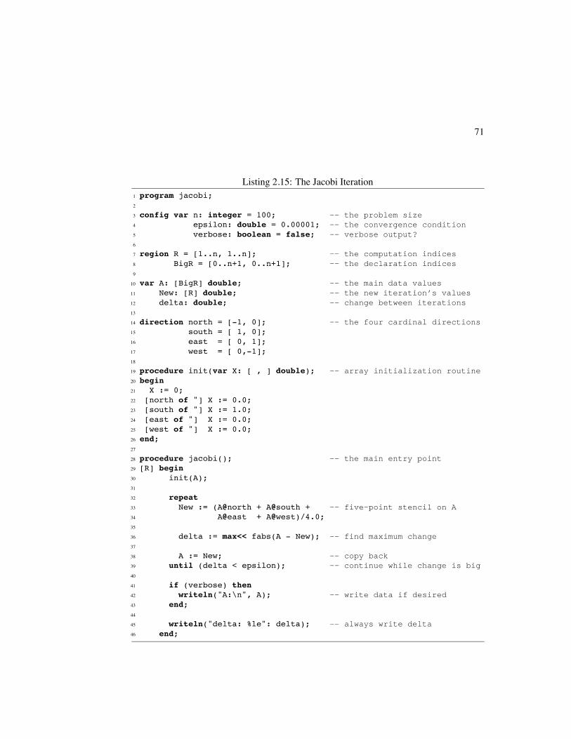
Listing 2.15 shows an implementation of the Jacobi iteration in ZPL. This code makes
use of many of the concepts that this chapter introduced: configuration variables, regions,
directions, and parallel arrays; region inheritance using blank dimensions and double-quote
references; the @ operator and full reductions; promotion of scalars, operators, and proce-
dures; and I/O.
The code begins with the program statement, which names the program and identifies
the code’s entry procedure. Lines 3–5 declare three configuration variables: n, which serves
as the size of the grid; epsilon which specifies the termination condition; and verbose
which indicates whether or not to print verbose output during the program’s run.
Lines 7–8 declare two regions for the program. The first, R, is the region which specifies
the size of the regular grid. The second region, BigR, is used to declare the main data array,
which requires an extra row and column in each direction to store boundary values.
71
Listing 2.15: The Jacobi Iteration1 program jacobi;2
3 config var n: integer = 100; -- the problem size4 epsilon: double = 0.00001; -- the convergence condition5 verbose: boolean = false; -- verbose output?6
7 region R = [1..n, 1..n]; -- the computation indices8 BigR = [0..n+1, 0..n+1]; -- the declaration indices9
10 var A: [BigR] double; -- the main data values11 New: [R] double; -- the new iteration’s values12 delta: double; -- change between iterations13
14 direction north = [-1, 0]; -- the four cardinal directions15 south = [ 1, 0];16 east = [ 0, 1];17 west = [ 0,-1];18
19 procedure init(var X: [ , ] double); -- array initialization routine20 begin21 X := 0;22 [north of "] X := 0.0;23 [south of "] X := 1.0;24 [east of "] X := 0.0;25 [west of "] X := 0.0;26 end;27
28 procedure jacobi(); -- the main entry point29 [R] begin30 init(A);31
32 repeat33 New := (A@north + A@south + -- five-point stencil on A34 A@east + A@west)/4.0;35
36 delta := max<< fabs(A - New); -- find maximum change37
38 A := New; -- copy back39 until (delta < epsilon); -- continue while change is big40
41 if (verbose) then42 writeln("A:\n", A); -- write data if desired43 end;44
45 writeln("delta: %le": delta); -- always write delta46 end;
72
Lines 10–12 declare the variables for the problem. Array A serves as the primary data
array, which is declared over region BigR to store the boundary values. Array New stores
the new values computed during each iteration and requires no boundary values, so it is
declared using region R. The variable delta is a scalar value that is used to store the
maximum change that an array value undergoes in a single iteration.
Lines 14–17 declare the four cardinal directions, used to express the five-point stencil.
Lines 19–26 declare a procedure init() that is used to initialize the data array A.
Note that this procedure is written in a generic manner for two-dimensional arrays, taking a
2D array of any size as its input parameter and containing statements that rely on dynamic
region inheritance. The procedure zeroes out the array for all indices specified by the
dynamically enclosing region scope, as well as its north, east, and west boundaries. The
southern boundary is initialized to 1.0.
The main procedure spans lines 28–46. It opens a region scope using R that supplies
indices to all parallel expressions within the procedure. It also serves as the enclosing
region for the call to init() on line 30.
The main computation takes place in lines 32–39. Lines 33-34 compute the 5-point
stencil on A using the @ operator and the four cardinal directions. The result is stored in
the array New. Next, in line 36, the scalar fabs() routine is promoted across the array
expression A - New. The fabs() routine is part of the standard C library and is included
in ZPL’s standard context. This computes the absolute value of the difference between
corresponding elements of A and New. The resulting array of values is then collapsed to
a scalar using the max reduction operator, and assigned to delta. The new values are
assigned back into A in preparation for the next iteration in line 38. This loop is repeated
until delta falls below the convergence value, epsilon.
Lines 41–45 output the results. If the verbose flag is true, line 42 prints the values
of A described by R to the console in row-major order. The final value of delta is printed
using exponential notation in line 45 and the program exits.
73
2.15.2 Matrix-Vector Multiplication
Matrix-vector multiplication is a fundamental operation that is used in a wide variety of
numerical computations. This section considers two possible implementations using 2D
and 1D vector representations.
2D Vector Implementation
Listing 2.16 shows an implementation of matrix-vector multiplication in ZPL. Though a
fairly simple program, it demonstrates the use of flood dimensions, file I/O, partial reduc-
tions, and the remap operator.
Typically, matrices are thought of as being 2-dimensional while vectors are considered
1-dimensional. However, since ZPL makes interactions between 1D and 2D arrays non-
trivial, this program represents all vectors using 2D arrays with either a flood or singleton
dimension. In particular, it uses a flooded row array to store the vector argument so that its
values will conform to all rows of the matrix.
Lines 3–5 declare the configuration variables. The values m and n are used to repre-
sent the number of rows and columns of the matrix, respectively. The third configuration
variable is of the string type and stores the filename for reading the matrix and vector.
Lines 7–10 declare the regions for this program. Region R is the base region which
describes the matrix indices. Lines 8–9 declare two row regions: TopRow, a singleton row,
and RowVect, a flooded row. Line 10 declares a singleton column region, ColVect, that
describes the result of the multiplication. Arrays are declared for each region in lines 12–15.
The matvectmult() procedure itself spans lines 17–34. Lines 20–23 open the file
specified by the filename configuration variable and read values for matrix M and input
vector I from it. Line 25 uses the flood operator to assign a replicated copy of the input
vector to V, the flooded vector. Note that the source region for the flood is a dynamic region
that inherits its second dimension from RowVect. Equivalently, the region TopRow could
have served as the source region. The dynamic region is used here for illustrative purposes.
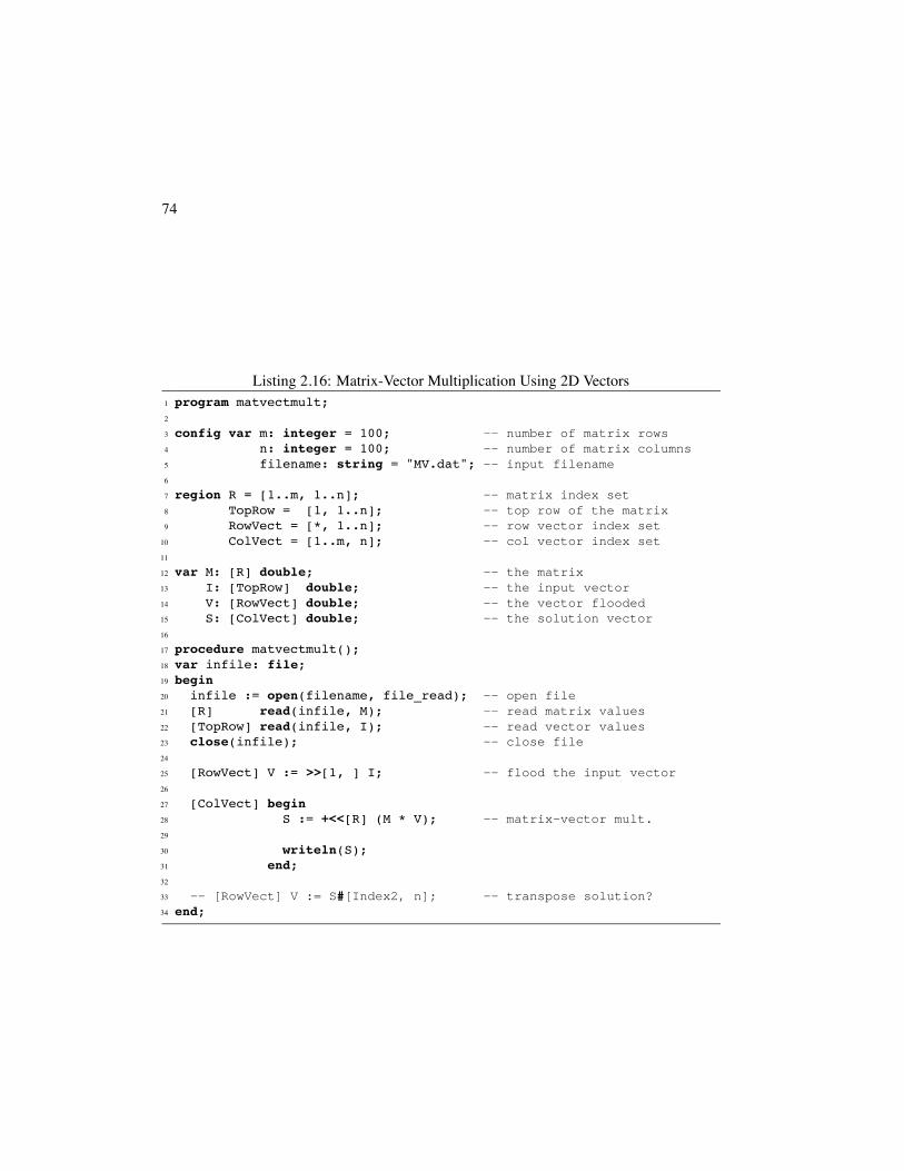
74
Listing 2.16: Matrix-Vector Multiplication Using 2D Vectors1 program matvectmult;2
3 config var m: integer = 100; -- number of matrix rows4 n: integer = 100; -- number of matrix columns5 filename: string = "MV.dat"; -- input filename6
7 region R = [1..m, 1..n]; -- matrix index set8 TopRow = [1, 1..n]; -- top row of the matrix9 RowVect = [*, 1..n]; -- row vector index set
10 ColVect = [1..m, n]; -- col vector index set11
12 var M: [R] double; -- the matrix13 I: [TopRow] double; -- the input vector14 V: [RowVect] double; -- the vector flooded15 S: [ColVect] double; -- the solution vector16
17 procedure matvectmult();18 var infile: file;19 begin20 infile := open(filename, file_read); -- open file21 [R] read(infile, M); -- read matrix values22 [TopRow] read(infile, I); -- read vector values23 close(infile); -- close file24
25 [RowVect] V := >>[1, ] I; -- flood the input vector26
27 [ColVect] begin28 S := +<<[R] (M * V); -- matrix-vector mult.29
30 writeln(S);31 end;32
33 -- [RowVect] V := S#[Index2, n]; -- transpose solution?34 end;
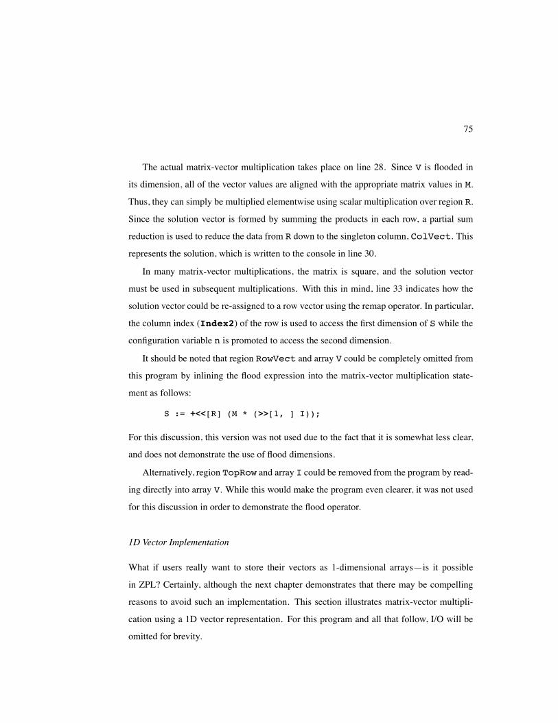
75
The actual matrix-vector multiplication takes place on line 28. Since V is flooded in
its dimension, all of the vector values are aligned with the appropriate matrix values in M.
Thus, they can simply be multiplied elementwise using scalar multiplication over region R.
Since the solution vector is formed by summing the products in each row, a partial sum
reduction is used to reduce the data from R down to the singleton column, ColVect. This
represents the solution, which is written to the console in line 30.
In many matrix-vector multiplications, the matrix is square, and the solution vector
must be used in subsequent multiplications. With this in mind, line 33 indicates how the
solution vector could be re-assigned to a row vector using the remap operator. In particular,
the column index (Index2) of the row is used to access the first dimension of S while the
configuration variable n is promoted to access the second dimension.
It should be noted that region RowVect and array V could be completely omitted from
this program by inlining the flood expression into the matrix-vector multiplication state-
ment as follows:
S := +<<[R] (M * (>>[1, ] I));
For this discussion, this version was not used due to the fact that it is somewhat less clear,
and does not demonstrate the use of flood dimensions.
Alternatively, region TopRow and array I could be removed from the program by read-
ing directly into array V. While this would make the program even clearer, it was not used
for this discussion in order to demonstrate the flood operator.
1D Vector Implementation
What if users really want to store their vectors as 1-dimensional arrays—is it possible
in ZPL? Certainly, although the next chapter demonstrates that there may be compelling
reasons to avoid such an implementation. This section illustrates matrix-vector multipli-
cation using a 1D vector representation. For this program and all that follow, I/O will be
omitted for brevity.
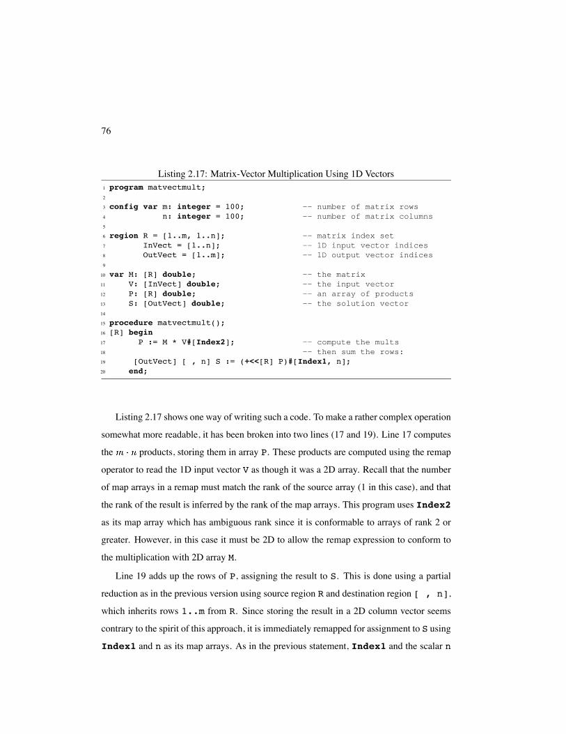
76
Listing 2.17: Matrix-Vector Multiplication Using 1D Vectors1 program matvectmult;2
3 config var m: integer = 100; -- number of matrix rows4 n: integer = 100; -- number of matrix columns5
6 region R = [1..m, 1..n]; -- matrix index set7 InVect = [1..n]; -- 1D input vector indices8 OutVect = [1..m]; -- 1D output vector indices9
10 var M: [R] double; -- the matrix11 V: [InVect] double; -- the input vector12 P: [R] double; -- an array of products13 S: [OutVect] double; -- the solution vector14
15 procedure matvectmult();16 [R] begin17 P := M * V#[Index2]; -- compute the mults18 -- then sum the rows:19 [OutVect] [ , n] S := (+<<[R] P)#[Index1, n];20 end;
Listing 2.17 shows one way of writing such a code. To make a rather complex operation
somewhat more readable, it has been broken into two lines (17 and 19). Line 17 computes
the products, storing them in array P. These products are computed using the remap
operator to read the 1D input vector V as though it was a 2D array. Recall that the number
of map arrays in a remap must match the rank of the source array (1 in this case), and that
the rank of the result is inferred by the rank of the map arrays. This program uses Index2
as its map array which has ambiguous rank since it is conformable to arrays of rank 2 or
greater. However, in this case it must be 2D to allow the remap expression to conform to
the multiplication with 2D array M.
Line 19 adds up the rows of P, assigning the result to S. This is done using a partial
reduction as in the previous version using source region R and destination region [ , n],
which inherits rows 1..m from R. Since storing the result in a 2D column vector seems
contrary to the spirit of this approach, it is immediately remapped for assignment to S using
Index1 and n as its map arrays. As in the previous statement, Index1 and the scalar n
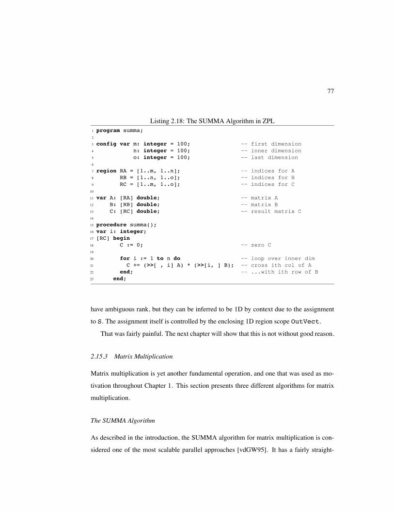
77
Listing 2.18: The SUMMA Algorithm in ZPL1 program summa;2
3 config var m: integer = 100; -- first dimension4 n: integer = 100; -- inner dimension5 o: integer = 100; -- last dimension6
7 region RA = [1..m, 1..n]; -- indices for A8 RB = [1..n, 1..o]; -- indices for B9 RC = [1..m, 1..o]; -- indices for C
10
11 var A: [RA] double; -- matrix A12 B: [RB] double; -- matrix B13 C: [RC] double; -- result matrix C14
15 procedure summa();16 var i: integer;17 [RC] begin18 C := 0; -- zero C19
20 for i := 1 to n do -- loop over inner dim21 C += (>>[ , i] A) * (>>[i, ] B); -- cross ith col of A22 end; -- ...with ith row of B23 end;
have ambiguous rank, but they can be inferred to be 1D by context due to the assignment
to S. The assignment itself is controlled by the enclosing 1D region scope OutVect.
That was fairly painful. The next chapter will show that this is not without good reason.
2.15.3 Matrix Multiplication
Matrix multiplication is yet another fundamental operation, and one that was used as mo-
tivation throughout Chapter 1. This section presents three different algorithms for matrix
multiplication.
The SUMMA Algorithm
As described in the introduction, the SUMMA algorithm for matrix multiplication is con-
sidered one of the most scalable parallel approaches [vdGW95]. It has a fairly straight-
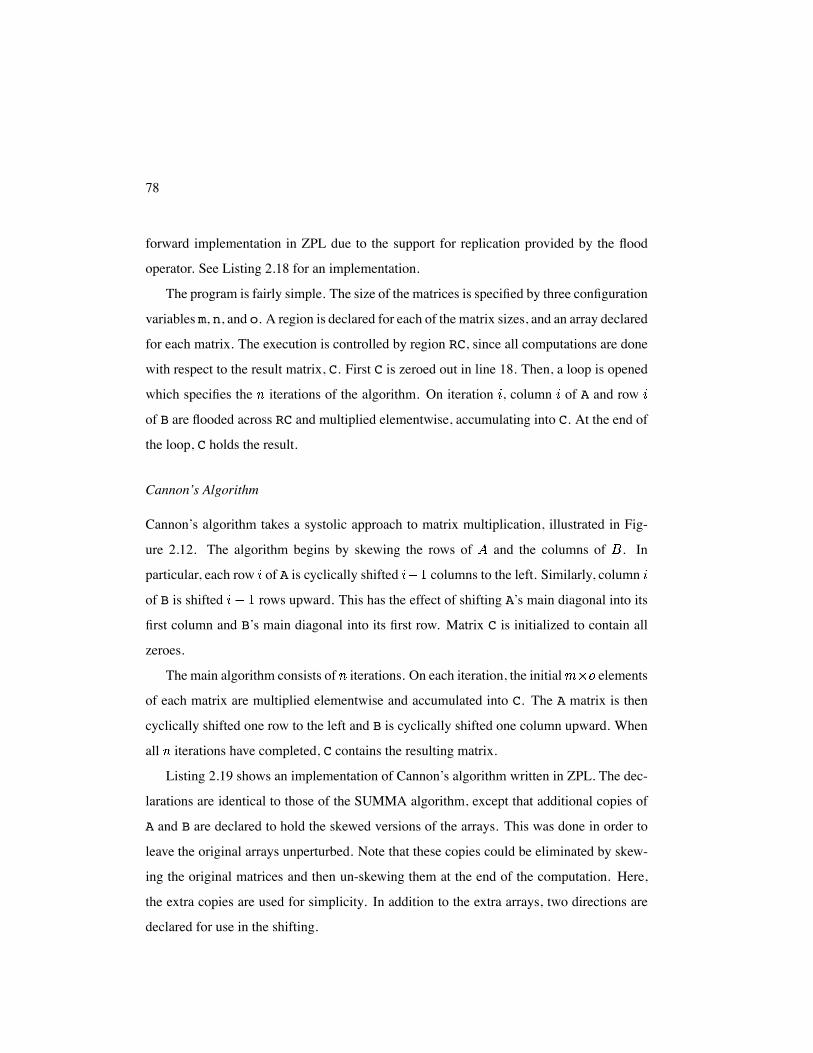
78
forward implementation in ZPL due to the support for replication provided by the flood
operator. See Listing 2.18 for an implementation.
The program is fairly simple. The size of the matrices is specified by three configuration
variables m, n, and o. A region is declared for each of the matrix sizes, and an array declared
for each matrix. The execution is controlled by region RC, since all computations are done
with respect to the result matrix, C. First C is zeroed out in line 18. Then, a loop is opened
which specifies the iterations of the algorithm. On iteration , column of A and row
of B are flooded across RC and multiplied elementwise, accumulating into C. At the end of
the loop, C holds the result.
Cannon’s Algorithm
Cannon’s algorithm takes a systolic approach to matrix multiplication, illustrated in Fig-
ure 2.12. The algorithm begins by skewing the rows of and the columns of . In
particular, each row of A is cyclically shifted columns to the left. Similarly, column
of B is shifted rows upward. This has the effect of shifting A’s main diagonal into its
first column and B’s main diagonal into its first row. Matrix C is initialized to contain all
zeroes.
The main algorithm consists of iterations. On each iteration, the initial elements
of each matrix are multiplied elementwise and accumulated into C. The A matrix is then
cyclically shifted one row to the left and B is cyclically shifted one column upward. When
all iterations have completed, C contains the resulting matrix.
Listing 2.19 shows an implementation of Cannon’s algorithm written in ZPL. The dec-
larations are identical to those of the SUMMA algorithm, except that additional copies of
A and B are declared to hold the skewed versions of the arrays. This was done in order to
leave the original arrays unperturbed. Note that these copies could be eliminated by skew-
ing the original matrices and then un-skewing them at the end of the computation. Here,
the extra copies are used for simplicity. In addition to the extra arrays, two directions are
declared for use in the shifting.
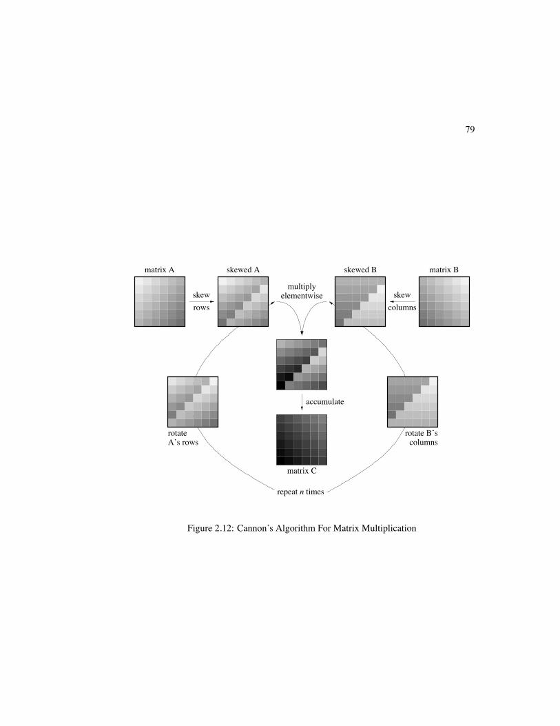
79
nrepeat times
multiplyelementwise
skewed B matrix Bskewed Amatrix A
accumulate
matrix C
rotateA’s rows
rowsskew skew
columns
rotate B’scolumns
Figure 2.12: Cannon’s Algorithm For Matrix Multiplication
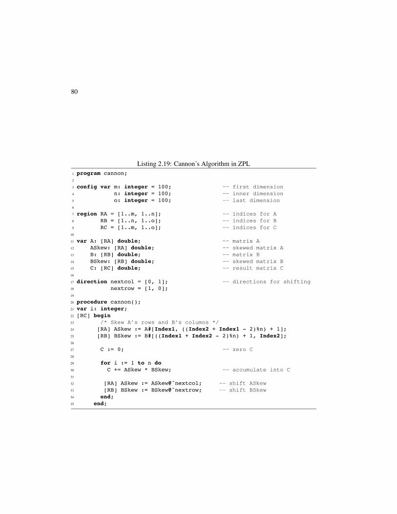
80
Listing 2.19: Cannon’s Algorithm in ZPL1 program cannon;2
3 config var m: integer = 100; -- first dimension4 n: integer = 100; -- inner dimension5 o: integer = 100; -- last dimension6
7 region RA = [1..m, 1..n]; -- indices for A8 RB = [1..n, 1..o]; -- indices for B9 RC = [1..m, 1..o]; -- indices for C
10
11 var A: [RA] double; -- matrix A12 ASkew: [RA] double; -- skewed matrix A13 B: [RB] double; -- matrix B14 BSkew: [RB] double; -- skewed matrix B15 C: [RC] double; -- result matrix C16
17 direction nextcol = [0, 1]; -- directions for shifting18 nextrow = [1, 0];19
20 procedure cannon();21 var i: integer;22 [RC] begin23 /* Skew A’s rows and B’s columns */24 [RA] ASkew := A#[Index1, ((Index2 + Index1 - 2)%n) + 1];25 [RB] BSkew := B#[((Index1 + Index2 - 2)%n) + 1, Index2];26
27 C := 0; -- zero C28
29 for i := 1 to n do30 C += ASkew * BSkew; -- accumulate into C31
32 [RA] ASkew := ASkew@ˆnextcol; -- shift ASkew33 [RB] BSkew := BSkew@ˆnextrow; -- shift BSkew34 end;35 end;
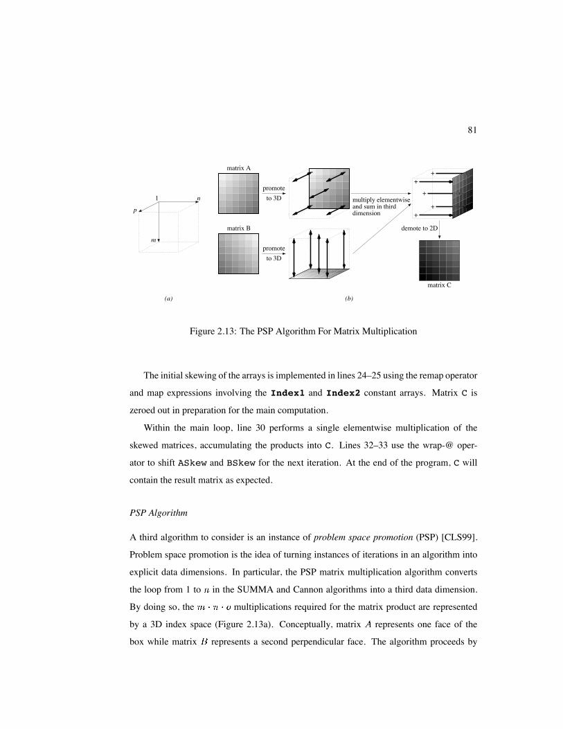
81
++
+
++
demote to 2D
1
(a) (b)
n
m
p
to 3Dpromote
to 3Dpromote
multiply elementwiseand sum in thirddimension
matrix A
matrix B
matrix C
Figure 2.13: The PSP Algorithm For Matrix Multiplication
The initial skewing of the arrays is implemented in lines 24–25 using the remap operator
and map expressions involving the Index1 and Index2 constant arrays. Matrix C is
zeroed out in preparation for the main computation.
Within the main loop, line 30 performs a single elementwise multiplication of the
skewed matrices, accumulating the products into C. Lines 32–33 use the wrap-@ oper-
ator to shift ASkew and BSkew for the next iteration. At the end of the program, C will
contain the result matrix as expected.
PSP Algorithm
A third algorithm to consider is an instance of problem space promotion (PSP) [CLS99].
Problem space promotion is the idea of turning instances of iterations in an algorithm into
explicit data dimensions. In particular, the PSP matrix multiplication algorithm converts
the loop from 1 to in the SUMMA and Cannon algorithms into a third data dimension.
By doing so, the multiplications required for the matrix product are represented
by a 3D index space (Figure 2.13a). Conceptually, matrix represents one face of the
box while matrix represents a second perpendicular face. The algorithm proceeds by
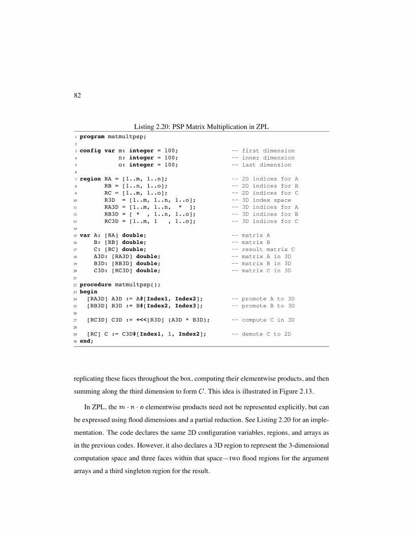
82
Listing 2.20: PSP Matrix Multiplication in ZPL1 program matmultpsp;2
3 config var m: integer = 100; -- first dimension4 n: integer = 100; -- inner dimension5 o: integer = 100; -- last dimension6
7 region RA = [1..m, 1..n]; -- 2D indices for A8 RB = [1..n, 1..o]; -- 2D indices for B9 RC = [1..m, 1..o]; -- 2D indices for C
10 R3D = [1..m, 1..n, 1..o]; -- 3D index space11 RA3D = [1..m, 1..n, * ]; -- 3D indices for A12 RB3D = [ * , 1..n, 1..o]; -- 3D indices for B13 RC3D = [1..m, 1 , 1..o]; -- 3D indices for C14
15 var A: [RA] double; -- matrix A16 B: [RB] double; -- matrix B17 C: [RC] double; -- result matrix C18 A3D: [RA3D] double; -- matrix A in 3D19 B3D: [RB3D] double; -- matrix B in 3D20 C3D: [RC3D] double; -- matrix C in 3D21
22 procedure matmultpsp();23 begin24 [RA3D] A3D := A#[Index1, Index2]; -- promote A to 3D25 [RB3D] B3D := B#[Index2, Index3]; -- promote B to 3D26
27 [RC3D] C3D := +<<[R3D] (A3D * B3D); -- compute C in 3D28
29 [RC] C := C3D#[Index1, 1, Index2]; -- demote C to 2D30 end;
replicating these faces throughout the box, computing their elementwise products, and then
summing along the third dimension to form . This idea is illustrated in Figure 2.13.
In ZPL, the elementwise products need not be represented explicitly, but can
be expressed using flood dimensions and a partial reduction. See Listing 2.20 for an imple-
mentation. The code declares the same 2D configuration variables, regions, and arrays as
in the previous codes. However, it also declares a 3D region to represent the 3-dimensional
computation space and three faces within that space—two flood regions for the argument
arrays and a third singleton region for the result.
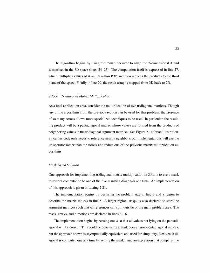
83
The algorithm begins by using the remap operator to align the 2-dimensional A and
B matrices in the 3D space (lines 24–25). The computation itself is expressed in line 27,
which multiplies values of A and B within R3D and then reduces the products to the third
plane of the space. Finally in line 29, the result array is mapped from 3D back to 2D.
2.15.4 Tridiagonal Matrix Multiplication
As a final application area, consider the multiplication of two tridiagonal matrices. Though
any of the algorithms from the previous section can be used for this problem, the presence
of so many zeroes allows more specialized techniques to be used. In particular, the result-
ing product will be a pentadiagonal matrix whose values are formed from the products of
neighboring values in the tridiagonal argument matrices. See Figure 2.14 for an illustration.
Since this code only needs to reference nearby neighbors, our implementations will use the
@ operator rather than the floods and reductions of the previous matrix multiplication al-
gorithms.
Mask-based Solution
One approach for implementing tridiagonal matrix multiplication in ZPL is to use a mask
to restrict computation to one of the five resulting diagonals at a time. An implementation
of this approach is given in Listing 2.21.
The implementation begins by declaring the problem size in line 3 and a region to
describe the matrix indices in line 5. A larger region, BigR is also declared to store the
argument matrices such that @-references can spill outside of the main problem area. The
mask, arrays, and directions are declared in lines 8–16.
The implementation begins by zeroing out C so that all values not lying on the pentadi-
agonal will be correct. This could be done using a mask over all non-pentadiagonal indices,
but the approach shown is asymptotically equivalent and used for simplicity. Next, each di-
agonal is computed one at a time by setting the mask using an expression that compares the
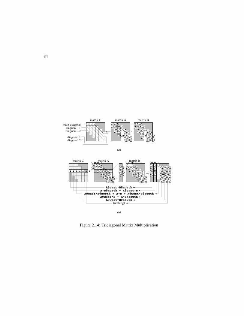
84
(a)
(b)
A@east*B@northA*B@north + A@east*B
A@east*B@north + A*B + A@west*B@southA@west*B + A*B@south
(nothing)A@west*B@south
matrix C matrix A matrix B
diagonal −2diagonal −1
main diagonal
diagonal 1diagonal 2
matrix C matrix A matrix B
Figure 2.14: Tridiagonal Matrix Multiplication
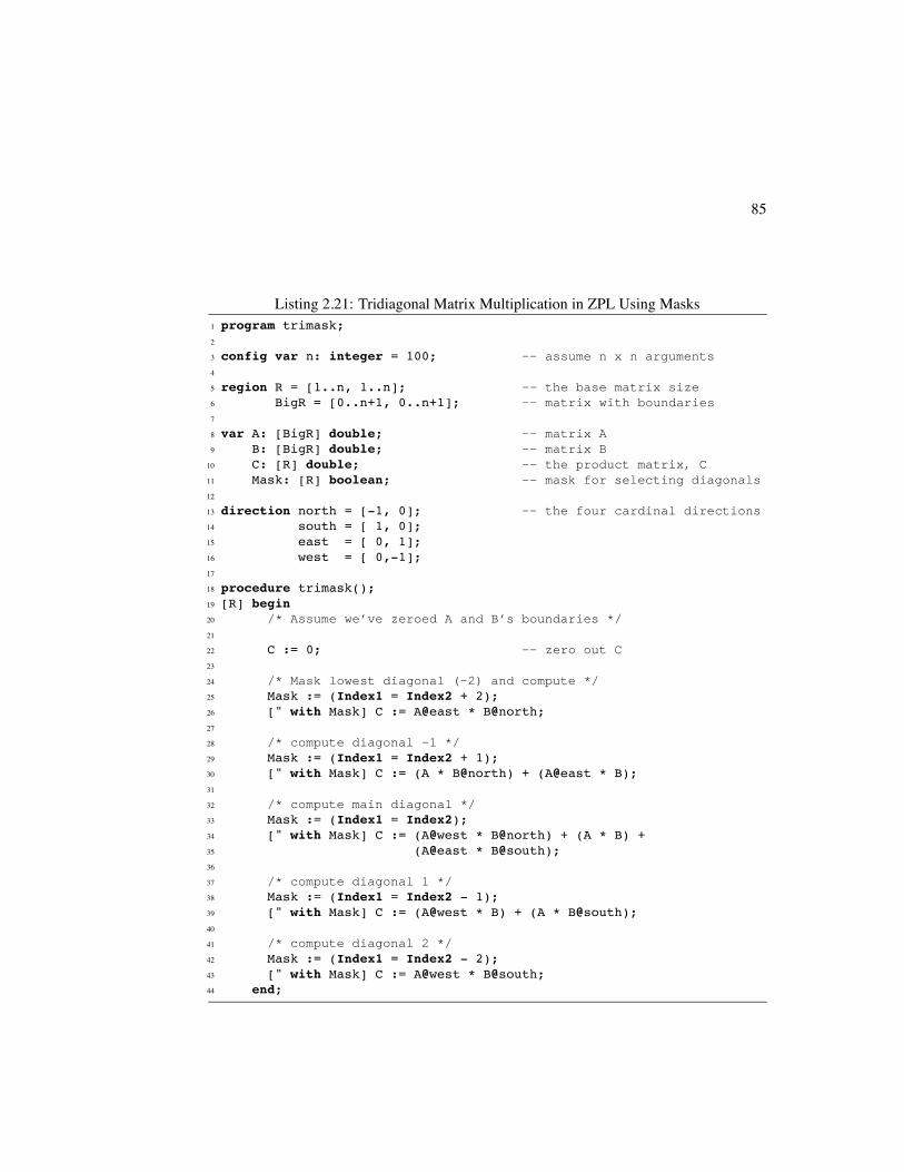
85
Listing 2.21: Tridiagonal Matrix Multiplication in ZPL Using Masks1 program trimask;2
3 config var n: integer = 100; -- assume n x n arguments4
5 region R = [1..n, 1..n]; -- the base matrix size6 BigR = [0..n+1, 0..n+1]; -- matrix with boundaries7
8 var A: [BigR] double; -- matrix A9 B: [BigR] double; -- matrix B
10 C: [R] double; -- the product matrix, C11 Mask: [R] boolean; -- mask for selecting diagonals12
13 direction north = [-1, 0]; -- the four cardinal directions14 south = [ 1, 0];15 east = [ 0, 1];16 west = [ 0,-1];17
18 procedure trimask();19 [R] begin20 /* Assume we’ve zeroed A and B’s boundaries */21
22 C := 0; -- zero out C23
24 /* Mask lowest diagonal (-2) and compute */25 Mask := (Index1 = Index2 + 2);26 [" with Mask] C := A@east * B@north;27
28 /* compute diagonal -1 */29 Mask := (Index1 = Index2 + 1);30 [" with Mask] C := (A * B@north) + (A@east * B);31
32 /* compute main diagonal */33 Mask := (Index1 = Index2);34 [" with Mask] C := (A@west * B@north) + (A * B) +35 (A@east * B@south);36
37 /* compute diagonal 1 */38 Mask := (Index1 = Index2 - 1);39 [" with Mask] C := (A@west * B) + (A * B@south);40
41 /* compute diagonal 2 */42 Mask := (Index1 = Index2 - 2);43 [" with Mask] C := A@west * B@south;44 end;
86
Index1 and Index2 arrays. The computation of each diagonal’s values is expressed in
a straightforward manner, using the mask to restrict it to the appropriate values. At the end
of the program, C contains the matrix product.
Shattered Control Flow Solution
A second implementation is very similar to the first, but uses shattered control flow rather
than a mask. The obvious advantage is that no time or space are required to compute and
store the mask.
The declarations are identical to the mask-based version. The main computation con-
sists of a shattered conditional that branches based on the relative values of Index1 and
Index2. Since the comparison of these arrays implies that they can be of any rank greater
than 1, the body of the conditional is examined to determine that this is a 2-dimensional
conditional, due to its references to A, B, and C. Each branch of the conditional simply
assigns C using that diagonal’s definition. The else clause at the end causes all non-
pentadiagonal values to be zeroed out.
Compact Solution
The final implementation uses a more compact representation for the banded matrices. In
particular, it uses an region, Tri, to represent the tridiagonal matrices and an re-
gion, Pent, to represent the resulting pentadiagonal. The regions’ second dimensions refer
to the diagonal numbers rather than matrix columns, and are therefore numbered between
, as appropriate. Note that directions north and south have been transformed
to ne and sw to reflect this index space transformation. The tridiagonal region is also ex-
tended by an additional row in each direction to handle @-references that spill outside of
the array’s bounds.
The computation proceeds by opening a single dynamic region per diagonal which in-
herits its row dimension from the enclosing region, Pent. The expression to compute each
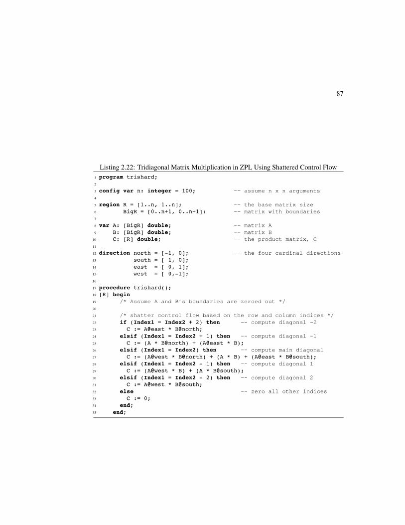
87
Listing 2.22: Tridiagonal Matrix Multiplication in ZPL Using Shattered Control Flow1 program trishard;2
3 config var n: integer = 100; -- assume n x n arguments4
5 region R = [1..n, 1..n]; -- the base matrix size6 BigR = [0..n+1, 0..n+1]; -- matrix with boundaries7
8 var A: [BigR] double; -- matrix A9 B: [BigR] double; -- matrix B
10 C: [R] double; -- the product matrix, C11
12 direction north = [-1, 0]; -- the four cardinal directions13 south = [ 1, 0];14 east = [ 0, 1];15 west = [ 0,-1];16
17 procedure trishard();18 [R] begin19 /* Assume A and B’s boundaries are zeroed out */20
21 /* shatter control flow based on the row and column indices */22 if (Index1 = Index2 + 2) then -- compute diagonal -223 C := A@east * B@north;24 elsif (Index1 = Index2 + 1) then -- compute diagonal -125 C := (A * B@north) + (A@east * B);26 elsif (Index1 = Index2) then -- compute main diagonal27 C := (A@west * B@north) + (A * B) + (A@east * B@south);28 elsif (Index1 = Index2 - 1) then -- compute diagonal 129 C := (A@west * B) + (A * B@south);30 elsif (Index1 = Index2 - 2) then -- compute diagonal 231 C := A@west * B@south;32 else -- zero all other indices33 C := 0;34 end;35 end;
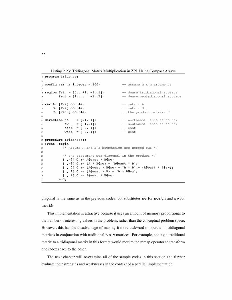
88
Listing 2.23: Tridiagonal Matrix Multiplication in ZPL Using Compact Arrays1 program tridense;2
3 config var n: integer = 100; -- assume n x n arguments4
5 region Tri = [0..n+1, -1..1]; -- dense tridiagonal storage6 Pent = [1..n, -2..2]; -- dense pentadiagonal storage7
8 var A: [Tri] double; -- matrix A9 B: [Tri] double; -- matrix B
10 C: [Pent] double; -- the product matrix, C11
12 direction ne = [-1, 1]; -- northeast (acts as north)13 sw = [ 1,-1]; -- southwest (acts as south)14 east = [ 0, 1]; -- east15 west = [ 0,-1]; -- west16
17 procedure tridense();18 [Pent] begin19 /* Assume A and B’s boundaries are zeroed out */20
21 /* one statement per diagonal in the product */22 [ ,-2] C := A@east * B@ne;23 [ ,-1] C := (A * B@ne) + (A@east * B);24 [ , 0] C := (A@west * B@ne) + (A * B) + (A@east * B@sw);25 [ , 1] C := (A@west * B) + (A * B@sw);26 [ , 2] C := A@west * B@sw;27 end;
diagonal is the same as in the previous codes, but substitutes ne for north and sw for
south.
This implementation is attractive because it uses an amount of memory proportional to
the number of interesting values in the problem, rather than the conceptual problem space.
However, this has the disadvantage of making it more awkward to operate on tridiagonal
matrices in conjunction with traditional matrices. For example, adding a traditional
matrix to a tridiagonal matrix in this format would require the remap operator to transform
one index space to the other.
The next chapter will re-examine all of the sample codes in this section and further
evaluate their strengths and weaknesses in the context of a parallel implementation.
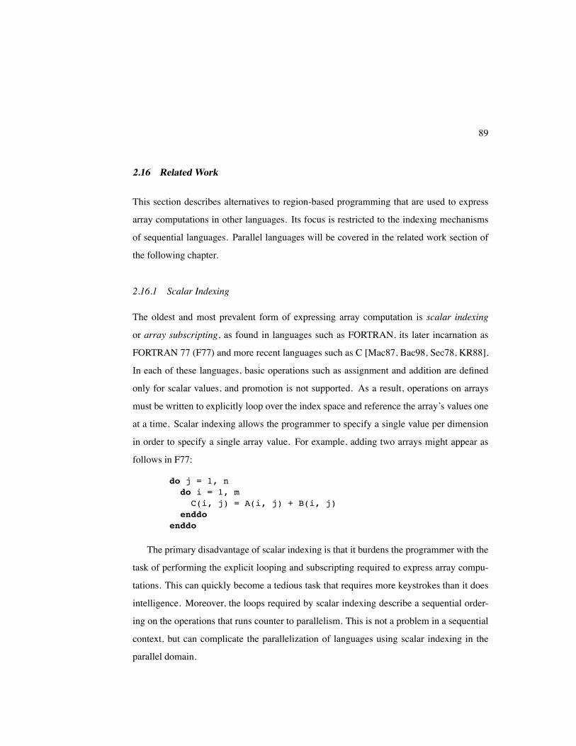
89
2.16 Related Work
This section describes alternatives to region-based programming that are used to express
array computations in other languages. Its focus is restricted to the indexing mechanisms
of sequential languages. Parallel languages will be covered in the related work section of
the following chapter.
2.16.1 Scalar Indexing
The oldest and most prevalent form of expressing array computation is scalar indexing
or array subscripting, as found in languages such as FORTRAN, its later incarnation as
FORTRAN 77 (F77) and more recent languages such as C [Mac87, Bac98, Sec78, KR88].
In each of these languages, basic operations such as assignment and addition are defined
only for scalar values, and promotion is not supported. As a result, operations on arrays
must be written to explicitly loop over the index space and reference the array’s values one
at a time. Scalar indexing allows the programmer to specify a single value per dimension
in order to specify a single array value. For example, adding two arrays might appear as
follows in F77:
do j = 1, ndo i = 1, mC(i, j) = A(i, j) + B(i, j)
enddoenddo
The primary disadvantage of scalar indexing is that it burdens the programmer with the
task of performing the explicit looping and subscripting required to express array compu-
tations. This can quickly become a tedious task that requires more keystrokes than it does
intelligence. Moreover, the loops required by scalar indexing describe a sequential order-
ing on the operations that runs counter to parallelism. This is not a problem in a sequential
context, but can complicate the parallelization of languages using scalar indexing in the
parallel domain.
90
Scalar indexing does have the advantage of being a very simple and general mechanism
for expressing array computations. For instance, there is no need for ZPL’s array operators,
nor its restrictions governing what types of expressions can and cannot interact. Moreover,
conformability rules in such a language are simple: since all arguments to an operator must
be scalars, the only check required is that all array dimensions are being indexed.
2.16.2 Vector Indexing
In the late 1950’s Kenneth Iverson developed a mathematical notation that was designed
to clarify some of the ambiguities that he felt standard mathematical notation contained.
Shortly thereafter, this notation evolved into APL (A Programming Language), one of the
earliest higher-level programming languages [Ive62, Mac87]. APL was the first pure array-
based programming language, since all data items in the language are arrays (scalars are
simply arrays of rank 0). APL’s arrays support vector indexing in which the programmer
supplies a vector of indices per dimension. The outer product of these vectors specifies the
indices of the array. In this way, array references no longer refer to a single value of the
array, but a subarray of values, or possibly the entire array. For example, matrix addition
would appear as follows in APL:
In this notation, represents a -element vector containing values from 0 to (sim-
ilar to ZPL’s Indexi arrays). Each element is incremented to use 1-based indexing to
be consistent with the Fortran implementation. Thus, the outer product of these vectors
causes each array reference to refer to elements . Addition ( ) and
assignment ( ) are promoted across the elements as in ZPL, and the sum is computed.
Although APL contained many elegant and revolutionary ideas, it has not remained in
widespread use over the years. Detractors find it too terse and unreadable, due primarily
to its large set of unique operators, most of which require non-standard characters (like the
“ ” used for assignment above). Though enthusiasts are quick to rush to its defense, it
91
remains largely unused and unknown today. Even so, its use of arrays as operators and
vector subscripting have had an influence on more modern languages including ZPL.
2.16.3 Array Slicing
Modern array-based languages have adopted syntax to support APL’s array operands with-
out so much generality and built-in support for mathematical operators. Many of these
languages have provided a syntax for accessing a regularly strided set of indices within
an array. This is known as array slicing or array sectioning, and represents an excellent
example of optimizing for the common case. Consider, for example, how few of the ZPL
programs from the previous section would require an APL-style index vector that was not
a simple -expression.
One language with support for array slicing is Fortran 90 (F90) [ABM 92], a successor
to F77. F90 allows the user to specify indices using a 3-tuple per dimension: [l:h:s].
These values are identical to the low, high, and stride values in ZPL’s sequence descriptors,
and they can be used to express a wide variety of simple APL-style -expressions. In F90,
serves as the alignment value, which was the fourth value in ZPL’s sequence descriptors.
Another language that supports slicing is Matlab, an interactive, interpreted matrix ma-
nipulation language [Mat93]. Matlab supports a slice notation similar to F90’s, but without
the stride value. In both languages, the low and high bounds may be omitted, which cause
the array’s declared bounds to be used. Omitting the stride in F90 results in a stride of 1.
Omitting the slice notation altogether causes the entire array to be referenced. Matrix addi-
tion would appear as follows in F90 and Matlab:
C(1:n, 1:n) = A(1:n, 1:n) + B(1:n, 1:n)
As in APL, both F90 and Matlab allow the programmer to use vector indexing, though
in practice this rarely seems to be used. For example, a five-element vector could be per-
muted in F90 using the following assignment:
X(1:5) = Y(/ 2,5,1,4,3 /)
92
Naturally, traditional scalar indexing may be used as well, should slicing or vector indexing
fail to express a desired array reference.
The primary advantage of array slicing over traditional indexing is that it is a more
concise means of specifying operations over arrays or subarrays, eliminating the need for
explicit loops for many array operations. Like scalar indexing, slices allow for more general
array interactions than ZPL’s regions, yet use a notation that is more concise and optimized
for the common case than that of APL’s vector indexing.
The chief disadvantage of array slicing is the syntactic overhead of specifying a region-
like set of indices for each array reference. Though small examples like matrix addition
are not so bad, slice notation can become rather cumbersome and error-prone in larger
array codes. In particular, the conformability requirements of array slices require the size
and shape of each array operand to match, causing redundant information to be supplied
with each array reference. Moreover, these conformability rules require more analysis
than scalar indexing or region-based indexing, both of which can be satisfied by simple
checks of the arguments (note that the related problem of bounds checking is common to
all approaches, and is not made simpler by any scheme).
2.16.4 Forall loops
A final array access mechanism that is often supported by languages to simplify scalar in-
dexing is the forall loop. This structure iterates over a multidimensional index range or
an arbitrary index set, typically in an unspecified order. In this sense, forall loops repre-
sent universal quantification much like regions, in that they generate a set of indices with
which to operate. Unlike regions, forall loops tend to use iterator variables like traditional
for loops. These iterators are typically used to access an array’s values using scalar index-
ing. Thus, forall loops can be considered a compact representation of a nested loop whose
iteration order is unconstrained.
FIDIL (FInite DIfference Language) [SH89, HC93] is an example of an array language
that uses forall loops. FIDIL was designed for use in scientific computation and supports
93
general index sets called domains. Domains need neither be rectangular nor dense, and
FIDIL supports computation over them using set-theoretic union, intersection, and differ-
ence operations. Domains are used both to specify the structure of arrays (maps), and to
provide index sets for FIDIL’s forall loops.
Fortran 95 [Geh96] also supports a forall loop structure that takes an array slice as its
bounds and iterates over the indices that it describes. In this context, the forall loop is much
more of a syntactic sugar, as there is no language-level support for index sets as in FIDIL
and ZPL.
2.17 Evaluation
To evaluate the impact of region-based programming on a program’s clarity, the sample
codes of this chapter are compared to sequential, hand-written implementations in C. Ap-
pendix A contains the source code for these C implementations for reference.
Each line of code in the ZPL and C implementations of the benchmarks is classified
as serving one of three purposes: (1) declaring a variable, procedure, or other identifier;
(2) computing the benchmark’s result; or (3) performing other non-essential work such as
I/O, initialization, timing, etc. This study only considers lines in the first two categories.
The graphs in Figures 2.15 and 2.16 indicate the number of useful lines and characters of
code used by each implementation. Characters were counted by removing all extraneous
spaces and whitespace from the codes, other than that which is required to represent the
algorithms in a simple, readable form.
The general trend shown in these graphs is that ZPL codes express computation with
a conciseness similar to C, both in terms of line- and character counts. These benchmarks
also indicate that the coding effort in the ZPL versions of these benchmarks tends to be
weighted more heavily towards declarations than computation. This is a result of ZPL’s use
of high-level named concepts like regions and directions to replace traditional loops and
indexing. Presumably, the overhead of these declarations will be lessened in longer codes
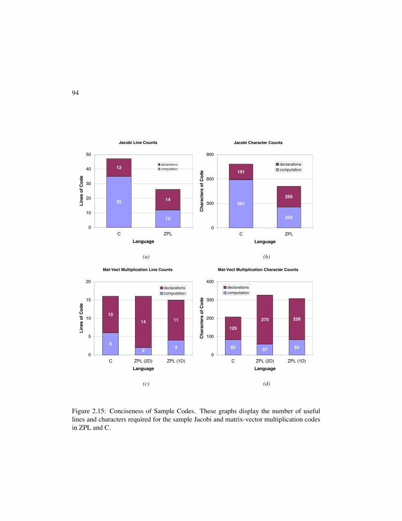
94
Jacobi Line Counts
12
35
12
14
0
10
20
30
40
50
C ZPLLanguage
Line
s of
Cod
e
declarationscomputation
(a)
Jacobi Character Counts
591
255
255
191
0
300
600
900
C ZPLLanguage
Char
acte
rs o
f Cod
e
declarationscomputation
(b)
Mat-Vect Multiplication Line Counts
26
4
1014 11
0
5
10
15
20
C ZPL (2D) ZPL (1D)Language
Line
s of
Cod
e
declarationscomputation
(c)
Mat-Vect Multiplication Character Counts
82
226
82 57
270
125
0
100
200
300
400
C ZPL (2D) ZPL (1D)Language
Char
acte
rs o
f Cod
e
declarationscomputation
(d)
Figure 2.15: Conciseness of Sample Codes. These graphs display the number of usefullines and characters required for the sample Jacobi and matrix-vector multiplication codesin ZPL and C.
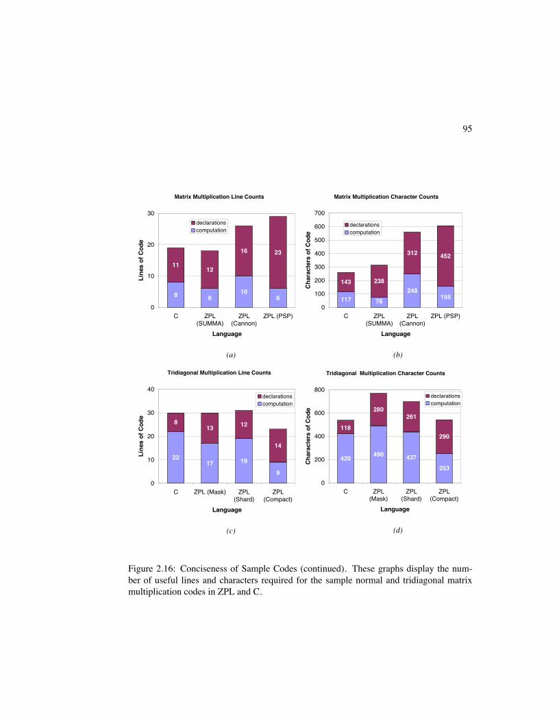
95
Matrix Multiplication Line Counts
6108 6
2316
1211
0
10
20
30
C ZPL(SUMMA)
ZPL(Cannon)
ZPL (PSP)
Language
Line
s of
Cod
e
declarationscomputation
(a)
Matrix Multiplication Character Counts
248155
312 452
76117
143 238
0
100
200
300
400
500
600
700
C ZPL(SUMMA)
ZPL(Cannon)
ZPL (PSP)
Language
Char
acte
rs o
f Cod
e
declarationscomputation
(b)
Tridiagonal Multiplication Line Counts
1722 19
9
813 12
14
0
10
20
30
40
C ZPL (Mask) ZPL(Shard)
ZPL(Compact)
Language
Line
s of
Cod
e
declarationscomputation
(c)
Tridiagonal Multiplication Character Counts
437253
261
290
490420
118
280
0
200
400
600
800
C ZPL(Mask)
ZPL(Shard)
ZPL(Compact)
Language
Char
acte
rs o
f Cod
e
declarationscomputation
(d)
Figure 2.16: Conciseness of Sample Codes (continued). These graphs display the num-ber of useful lines and characters required for the sample normal and tridiagonal matrixmultiplication codes in ZPL and C.
96
where the same declarations can be used again and again, amortizing the cost of declaring
them over a larger code base. The experiments in Chapters 5 and 6 support this hypothesis.
The following paragraphs give a few notes for each benchmark.
The Jacobi Iteration
The Jacobi Iteration best demonstrates the benefits of region-based programming. While
most of the other benchmarks consist of a small number of array statements surrounded
by a single region, the Jacobi benchmark uses a number of diverse regions to establish its
boundary conditions. In the C code, each of these regions requires its own loop, demon-
strating the region’s concise support for array computation. Since most real-world codes
will tend to require many regions/loop nests to express a computation, this benchmark best
demonstrates the concise power that a few appropriate ZPL declarations can have.
Matrix-Vector Multiplication
C and ZPL represent matrix-vector multiplication using reasonably equivalent code sizes.
Once again, the ZPL representations tend to be slightly more concise in terms of computa-
tion due to the use of regions rather than loops.
Matrix Multiplication
Matrix multiplication represents a worst-case for ZPL, simply due to the difference in com-
plexity between sequential and parallel matrix multiplication algorithms. In particular, se-
quential C algorithms can simply iterate over the matrices and compute on them in-place.
In contrast, all of the parallel algorithms described by this chapter require some amount of
data movement and copying.
The SUMMA algorithm is ZPL’s most concise implementation and the only one that is
more compact than C’s triply-nested loop. Cannon’s algorithm requires significantly more
computation due to its skewing operation and cyclic shifts. It also requires additional decla-
97
rations to create the directions used to implement the shifting. The PSP algorithm requires
the greatest amount of declarations due to its use of 2D and 3D regions to describe its two
computational domains. The PSP computation itself is fairly concise in terms of lines, but
these lines are long due to the Indexi expressions used to implement the alignment of
arrays from 2D to 3D.
Tridiagonal Matrix Multiplication
The hand-coded C implementation of tridiagonal matrix multiplication uses a compact rep-
resentation of the matrices similar to the third ZPL implementation. As a result, these
two codes are the most comparable in size due to their similar approach. ZPL’s mask- and
shard-based approaches tend to require more computation due to the overhead of restricting
computation to the diagonals within the logical 2D index space. In contrast, the compact
ZPL and C implementations can trivially isolate a single diagonal.
Summary
In summary, ZPL can represent these simple algorithms as concisely as C. ZPL tends to re-
quire slightly less syntax to specify computation due to its use of regions to replace looping
and indexing. This effect is offset somewhat by ZPL’s more verbose syntax (e.g., Indexi
constants, the use of begin...end rather than curly braces). For the benchmarks stud-
ied here, ZPL tends to require more declarations than C, though it is expected that these
declarations will be amortized in larger benchmarks by the savings in computation.
It is crucial to keep in mind that the ZPL implementations of this section differ from
the C codes in one crucial way: they represent fully-functional parallel implementations
of the benchmarks, whereas the C codes can only be run on a single processor. For this
reason, regions must be considered a benefit to clarity, since they support the expression of
a more complex program using syntax that tends to be as concise as sequential C. As the
next chapter will show, this cannot be said for most parallel languages.
98
2.18 Discussion
2.18.1 Benefits of Regions
Though Section 2.16 argued that regions are somewhat less flexible and adaptable than
array indexing and slicing, they are not without their benefits. This section describes the
advantages that regions give programmers, syntactically and semantically.
Cleaner Elementwise Operations
Performing strict elementwise operations on arrays remains an extremely common case
in array-based programming. Though interesting programs will require more complex in-
teractions between their arrays, most large programs will still require many elementwise
operations in addition to the more complex ones. In these cases, regions represent a posi-
tive evolution in array reference syntax. Array slices can be seen as a factoring of F77 loop
bounds into the array references in order to optimize the common case of iterating over
an array in a regular manner. In the same spirit, regions can be thought of as factoring a
set of indices that describe the size and shape of slice-based array references into a single
prefixing slice—the region scope.
Table 2.8 shows a number of simple array statements written in F77, F90, and ZPL.
In the first row, a simple array addition is demonstrated. The F77 version requires explicit
loops and repetitive array indexing. The F90 version eliminates the loops, but requires
identical slices to be applied to each individual array reference. The ZPL version factors this
common slice into the region scope, leaving the array references unadorned and eliminating
a lot of redundant typing. Since elementwise operations constitute a common case, the
result is that many array references will be unadorned in ZPL.
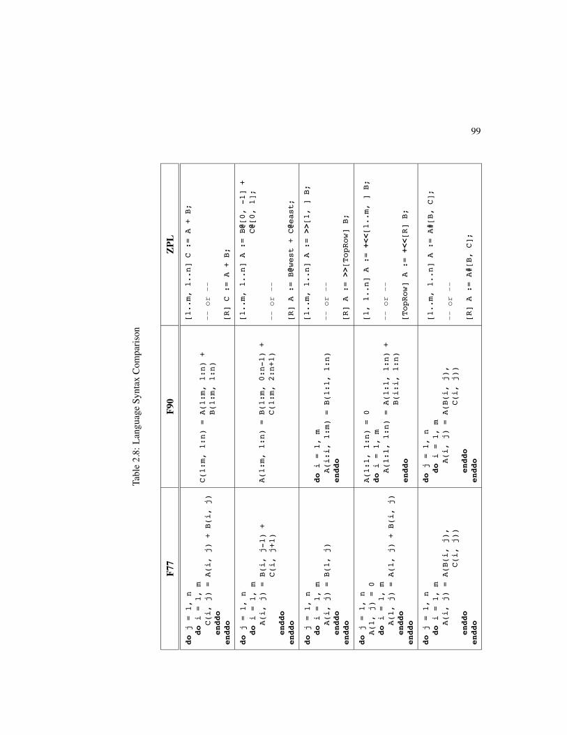
99Ta
ble
2.8:
Lang
uage
Synt
axCo
mpa
rison
F77
F90
ZPL
doj
=1,
ndo
i=
1,m
C(i,
j)=
A(i,
j)+
B(i,
j)en
ddo
endd
o
C(1:m,
1:n)
=A(1:m,
1:n)
+B(1:m,
1:n)
[1..m,
1..n]C
:=A
+B;
--
or
--
[R]
C:=
A+B;
doj
=1,
ndo
i=
1,m
A(i,
j)=
B(i,
j-1)
+C(i,
j+1)
endd
oen
ddo
A(1:m,
1:n)
=B(1:m,
0:n-1)
+C(1:m,
2:n+1)
[1..m,
1..n]A
:=B@
[0,-1]
+C@
[0,1];
--
or
--
[R]
A:=
B@west
+C@
east;
doj
=1,
ndo
i=
1,m
A(i,
j)=
B(1,
j)en
ddo
endd
o
doi
=1,
mA(i:i,
1:m)
=B(1:1,
1:n)
endd
o
[1..m,
1..n]A
:=>>
[1,]
B;
--
or
--
[R]
A:=
>>[TopRow]
B;
doj
=1,
nA(1,
j)=0
doi=
1,m
A(1,
j)=
A(1,
j)+
B(i,
j)en
ddo
endd
o
A(1:1,
1:n)
=0
doi
=1,
mA(1:1,
1:n)
=A(1:1,
1:n)
+B(i:i,
1:n)
endd
o
[1,1..n]
A:=
+<<[1..m,
]B;
--
or
--
[TopRow]
A:=
+<<[R]
B;
doj
=1,
ndo
i=
1,m
A(i,
j)=
A(B(i,
j),
C(i,
j))
endd
oen
ddo
doj
=1,
ndo
i=
1,m
A(i,
j)=
A(B(i,
j),
C(i,
j))
endd
oen
ddo
[1..m,
1..n]A
:=A#
[B,C];
--
or
--
[R]
A:=
A#[B,
C];
100
Clearer Array Reference Patterns
When array operations are not strictly elementwise, regions still serve a purpose by describ-
ing the size and shape of the subarray accesses. Array operators express any modifications
to these base indices for a particular array expression. This has the effect of syntactically
factoring the redundant part of each array reference out of the main computation, leaving
only indications of how each reference differs.
As an example, consider the second row of Table 2.8, in which shifted references to
and are summed. In F77 and F90, the array indices and slices encode redundant
information. In particular, F77 specifies that each access is based on index , while F90
specifies three slices, each of which are in size. In ZPL, the common aspects of
these array references—the base indices—are factored into the region, leaving only
the differences in how the arrays are accessed, using the @ operator. By removing much of
the redundant clutter, the meaning of the statement is clearer.
As further evidence, consider each column of the table one at a time to see how long
it takes you to identify the operation that is being performed by each statement. Note that
very different array operations end up looking rather similar in F77 and F90, whereas ZPL
does a better job of distinguishing them.
Fewer Loops Required
In F77, programmers expect to use loops and indices. In F90, many array operations no
longer require loops due to the availability of array slicing and vector indexing. However,
as the last two entries in Table 2.8 show, these mechanisms are not strong enough to express
floods, partial reductions, or remap operations without using loops. The floods and partial
reductions fail due to the requirement that the two sides of an operation must have the same
size and shape. This makes it illegal to add an arbitrary number of rows to a single row
without a loop. The remap operator cannot be written succinctly due to the fact that F90
has no mechanism for taking the dot product of vector indices rather than the cross product.
101
It should be noted that F90 supports intrinsic functions such as SUM, RESHAPE, and
TRANSPOSE that may be used to write such statements in a single line. However, these
functions should be considered part of a standard library context rather than a syntax-based
means for expressing array computation. Similarly, F95’s forall loops allow such state-
ments to be written on a single line, but still rely on a loop-style concept (albeit one that
syntactically begins to resemble the region).
Naming Improves Readability
The fact that regions can be named greatly improves the readability of ZPL code, since it
allows index sets to be given identifiers that are meaningful to the programmer. Column 3
in Table 2.8 shows each ZPL statement written both with and without identifiers. These
examples demonstrate that names can improve the clarity of each statement. Note that the
ability to name array slices or index ranges could improve the readability of F90 codes
somewhat, but would not produce a ZPL-equivalent syntax.
Regions Promote Code Reuse
The fact that regions are dynamically scoped allows procedures to be written in a more
generic way. As a simple example, note that the ZPL implementation of the SUMMA
algorithm (Figure 1.2) could be moved into a procedure that takes only the size of the
inner dimension as an argument and inherits the matrix size from the callsite. In contrast,
a generic F90 implementation would require the bounds for each dimension to be passed
in as arguments. Furthermore, even when an algorithm does require more than a single
inherited region (as in the Cannon and PSP algorithms), regions represent a concise means
of bundling index information for passing to another procedure.
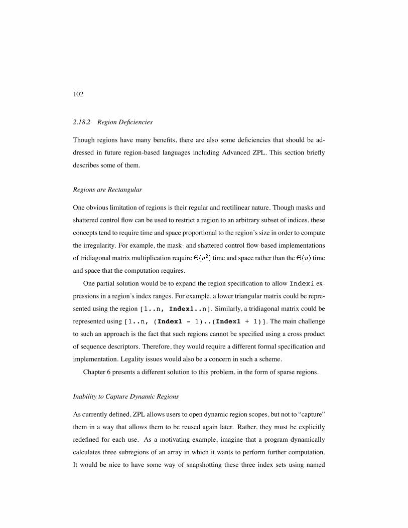
102
2.18.2 Region Deficiencies
Though regions have many benefits, there are also some deficiencies that should be ad-
dressed in future region-based languages including Advanced ZPL. This section briefly
describes some of them.
Regions are Rectangular
One obvious limitation of regions is their regular and rectilinear nature. Though masks and
shattered control flow can be used to restrict a region to an arbitrary subset of indices, these
concepts tend to require time and space proportional to the region’s size in order to compute
the irregularity. For example, the mask- and shattered control flow-based implementations
of tridiagonal matrix multiplication require time and space rather than the time
and space that the computation requires.
One partial solution would be to expand the region specification to allow Indexi ex-
pressions in a region’s index ranges. For example, a lower triangular matrix could be repre-
sented using the region [1..n, Index1..n]. Similarly, a tridiagonal matrix could be
represented using [1..n, (Index1 - 1)..(Index1 + 1)]. The main challenge
to such an approach is the fact that such regions cannot be specified using a cross product
of sequence descriptors. Therefore, they would require a different formal specification and
implementation. Legality issues would also be a concern in such a scheme.
Chapter 6 presents a different solution to this problem, in the form of sparse regions.
Inability to Capture Dynamic Regions
As currently defined, ZPL allows users to open dynamic region scopes, but not to “capture”
them in a way that allows them to be reused again later. Rather, they must be explicitly
redefined for each use. As a motivating example, imagine that a program dynamically
calculates three subregions of an array in which it wants to perform further computation.
It would be nice to have some way of snapshotting these three index sets using named
103
regions so that they could be reused later, rather than explicitly maintaining their bounds
using scalar variables.
This lack also makes it difficult to declare persistent arrays using a dynamic region.
Arrays that are local to a procedure may be declared using the dynamically covering region
or an explicit dynamic region, but such arrays will not persist once the procedure returns.
This restricts the user’s ability to declare an array over the three subregions of the previous
paragraph, for example, such that they could be used throughout the program naturally.
Inability to Redefine Regions
A related problem is that named regions cannot be redefined. In a sense, ZPL’s regions can
be viewed as constant sets of indices that cannot be altered during the program’s execution.
For some applications in which a problem size cannot be known at configuration time, it
would be nice to incrementally grow regions to meet a program’s specific requirements
dynamically. For example, while a 1D region can be used to implement an array-based
list in ZPL, the list cannot be grown using standard array resizing techniques because the
bounds of its defining region cannot be modified.
Regions are Inflexible
In ZPL, regions are technically neither a type, nor a first-class object. This limits their use
in a number of ways: programmers may not declare collections of regions using indexed ar-
rays or records; they may not assign regions; they may not pass regions to a procedure; etc.
This design choice was made in order to provide the compiler with as much information
about the regions as possible. The idea was to start with a restricted region definition and
then broaden it as much as the compiler could tolerate without sacrificing performance or
the ability to effectively parallelize a ZPL program. During the past decade, virtually no
relaxation of these restrictions has taken place, though it has seemed increasingly feasible
to do so.
104
2.18.3 Proposed Support for Regions as Values
One solution to many of the previous section’s problems would be to promote the region
concept to that of a first-class value. In doing so, traditional region declarations would be
interpreted as declarations of constant or configuration regions. That is, the following two
declarations would be considered equivalent to one another:
region R = [1..m, 1..n];config var R: region = [1..m, 1..n];
Any regions for which ZPL’s current rules are overly strict could be declared as variables
of type region, allowing them to be assigned dynamically, modified, or grown. Parallel
arrays declared using region variables would be reallocated after the region was assigned,
preserving any values in the intersection of the old and new index sets. Procedures could
be written with formal parameters of type region. Moreover, types could be created that
have region components, such as indexed arrays of regions and records with region fields.
The primary liability of this scheme is that current ZPL optimizations may be compro-
mised due to an increased amount of confusion over a region’s definition. For example,
in the presence of region assignments and aliasing, will the compiler be able to determine
whether a region’s dimension is floodable, singleton, or normal? What about its rank? It
seems reasonable to be optimistic about these issues since the absence of pointers should
make most of a region’s salient features statically detectable using interprocedural analysis.
Even in the worst-case, such an approach is worthy of more study in order to attempt to
support more general region-based programming.
2.18.4 Proposed Support for User-Defined Region Operators
One feature that I believe is missing from the ZPL language is the ability for users to
define their own region operators. While the region operators supported by ZPL form a
useful basis set, it is not difficult to conceive of other operators that might also benefit a
programmer. Rather than hoping to supply all region operators that a user could want, it
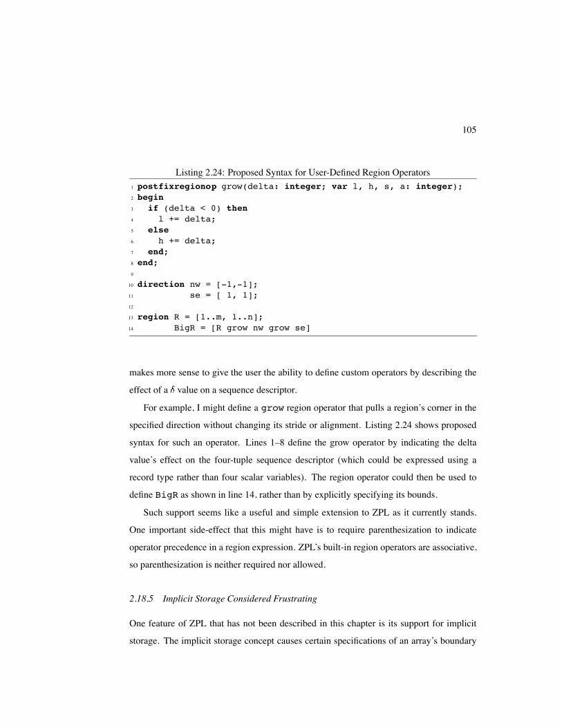
105
Listing 2.24: Proposed Syntax for User-Defined Region Operators1 postfixregionop grow(delta: integer; var l, h, s, a: integer);2 begin3 if (delta < 0) then4 l += delta;5 else6 h += delta;7 end;8 end;9
10 direction nw = [-1,-1];11 se = [ 1, 1];12
13 region R = [1..m, 1..n];14 BigR = [R grow nw grow se]
makes more sense to give the user the ability to define custom operators by describing the
effect of a value on a sequence descriptor.
For example, I might define a grow region operator that pulls a region’s corner in the
specified direction without changing its stride or alignment. Listing 2.24 shows proposed
syntax for such an operator. Lines 1–8 define the grow operator by indicating the delta
value’s effect on the four-tuple sequence descriptor (which could be expressed using a
record type rather than four scalar variables). The region operator could then be used to
define BigR as shown in line 14, rather than by explicitly specifying its bounds.
Such support seems like a useful and simple extension to ZPL as it currently stands.
One important side-effect that this might have is to require parenthesization to indicate
operator precedence in a region expression. ZPL’s built-in region operators are associative,
so parenthesization is neither required nor allowed.
2.18.5 Implicit Storage Considered Frustrating
One feature of ZPL that has not been described in this chapter is its support for implicit
storage. The implicit storage concept causes certain specifications of an array’s boundary
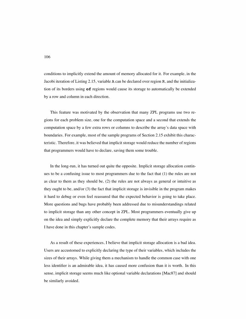
106
conditions to implicitly extend the amount of memory allocated for it. For example, in the
Jacobi iteration of Listing 2.15, variable A can be declared over region R, and the initializa-
tion of its borders using of regions would cause its storage to automatically be extended
by a row and column in each direction.
This feature was motivated by the observation that many ZPL programs use two re-
gions for each problem size, one for the computation space and a second that extends the
computation space by a few extra rows or columns to describe the array’s data space with
boundaries. For example, most of the sample programs of Section 2.15 exhibit this charac-
teristic. Therefore, it was believed that implicit storage would reduce the number of regions
that programmers would have to declare, saving them some trouble.
In the long-run, it has turned out quite the opposite. Implicit storage allocation contin-
ues to be a confusing issue to most programmers due to the fact that (1) the rules are not
as clear to them as they should be, (2) the rules are not always as general or intuitive as
they ought to be, and/or (3) the fact that implicit storage is invisible in the program makes
it hard to debug or even feel reassured that the expected behavior is going to take place.
More questions and bugs have probably been addressed due to misunderstandings related
to implicit storage than any other concept in ZPL. Most programmers eventually give up
on the idea and simply explicitly declare the complete memory that their arrays require as
I have done in this chapter’s sample codes.
As a result of these experiences, I believe that implicit storage allocation is a bad idea.
Users are accustomed to explicitly declaring the type of their variables, which includes the
sizes of their arrays. While giving them a mechanism to handle the common case with one
less identifier is an admirable idea, it has caused more confusion than it is worth. In this
sense, implicit storage seems much like optional variable declarations [Mac87] and should
be similarly avoided.
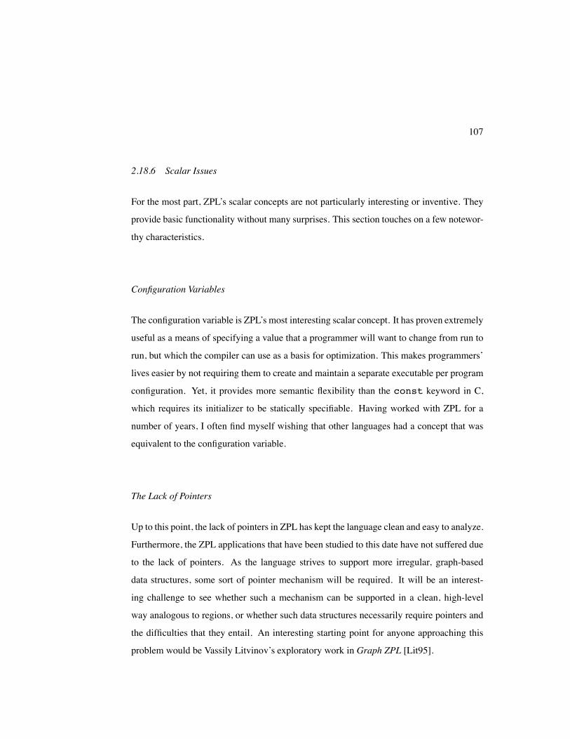
107
2.18.6 Scalar Issues
For the most part, ZPL’s scalar concepts are not particularly interesting or inventive. They
provide basic functionality without many surprises. This section touches on a few notewor-
thy characteristics.
Configuration Variables
The configuration variable is ZPL’s most interesting scalar concept. It has proven extremely
useful as a means of specifying a value that a programmer will want to change from run to
run, but which the compiler can use as a basis for optimization. This makes programmers’
lives easier by not requiring them to create and maintain a separate executable per program
configuration. Yet, it provides more semantic flexibility than the const keyword in C,
which requires its initializer to be statically specifiable. Having worked with ZPL for a
number of years, I often find myself wishing that other languages had a concept that was
equivalent to the configuration variable.
The Lack of Pointers
Up to this point, the lack of pointers in ZPL has kept the language clean and easy to analyze.
Furthermore, the ZPL applications that have been studied to this date have not suffered due
to the lack of pointers. As the language strives to support more irregular, graph-based
data structures, some sort of pointer mechanism will be required. It will be an interest-
ing challenge to see whether such a mechanism can be supported in a clean, high-level
way analogous to regions, or whether such data structures necessarily require pointers and
the difficulties that they entail. An interesting starting point for anyone approaching this
problem would be Vassily Litvinov’s exploratory work in Graph ZPL [Lit95].
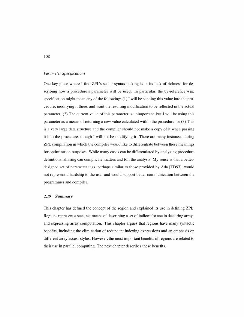
108
Parameter Specifications
One key place where I find ZPL’s scalar syntax lacking is in its lack of richness for de-
scribing how a procedure’s parameter will be used. In particular, the by-reference var
specification might mean any of the following: (1) I will be sending this value into the pro-
cedure, modifying it there, and want the resulting modification to be reflected in the actual
parameter; (2) The current value of this parameter is unimportant, but I will be using this
parameter as a means of returning a new value calculated within the procedure; or (3) This
is a very large data structure and the compiler should not make a copy of it when passing
it into the procedure, though I will not be modifying it. There are many instances during
ZPL compilation in which the compiler would like to differentiate between these meanings
for optimization purposes. While many cases can be differentiated by analyzing procedure
definitions, aliasing can complicate matters and foil the analysis. My sense is that a better-
designed set of parameter tags, perhaps similar to those provided by Ada [TD97], would
not represent a hardship to the user and would support better communication between the
programmer and compiler.
2.19 Summary
This chapter has defined the concept of the region and explained its use in defining ZPL.
Regions represent a succinct means of describing a set of indices for use in declaring arrays
and expressing array computation. This chapter argues that regions have many syntactic
benefits, including the elimination of redundant indexing expressions and an emphasis on
different array access styles. However, the most important benefits of regions are related to
their use in parallel computing. The next chapter describes these benefits.
Recommended