Chapter 2
LINEAR PROGRAMMINGPROBLEMS
2.1 Introduction
Linear Programming is the branch of applied mathematics that deals with solv-
ing optimization problems of a particular functional form. A linear programming
problem consists of a linear objective function (of decision variables) which is to
be minimized or maximized, subject to a certain set of linear constraints on de-
cision variables. The constraints are usually in the form of linear inequalities of
decision variables used in the objective function. Linear programming is a rel-
atively recent mathematical discipline. The Russian mathematician Leonid V.
Kantorovich formulated the first problem in linear programming in 1939. This
was what is now known as the transportation problem. The English economist
George Stigler (1945) described a problem of determining an optimal diet as a lin-
ear programming problem. The simplex algorithm was developed by the American
mathematician George B. Dantzig in 1947, and the theory of duality was developed
by John von Neumann the same year i.e. in 1947. It was also Dantzig who coined
the name ”‘Linear Programming”’ to this class of problems. In 1972, Klee and
Minty showed that the simplex method has exponential computational complex-
15

ity. In 1979, Khachiyan showed that linear programming problems can be solved
by polynomial time algorithms. Karmarkar, in 1984, described his interior-point
algorithm and claimed that it is a polynomial-time algorithm and works better
than Khachiyan’s algorithm.
What is common among all the algorithms mentioned above is that they are
all iterative and therefore sequential. That is, every subsequent solution depends
on a preceding solution. On one side, this introduces uniqueness in each of these
algorithms. On the other hand, however, the same feature makes these algorithms
rather restrictive. This chapter aims at developing a method that is neither se-
quential not restricted to the surface of the polytope representing the set of feasible
solutions of the linear programming problem. This development is motivated by
the need for a speedy algorithm, since each of the classical techniques often requires
a vast amount of calculations [15].
16
2.2 Linear Programming Problems in Canonical
Form
Linear programming problems can be expressed in the canonical form. The canon-
ical form of a linear programming problem is
Maximize C ′X (2.1)
subject to AX ≤ b, (2.2)
and X ≥ 0. (2.3)
Where C and X ∈ <n, b ∈ <m and A ∈ <m×n. Here (2.1) is called the
objective function, (2.2) is a system of linear inequation constraints and (2.3) is a
non-negativity constraint.
2.2.1 Features of linear programming problems
In this section we state some standard definitions and some of the important
characteristics of a solution to a linear programming problem formulated in the
canonical form.
• Feasible solution set. A set of values of the decision variables x1, x2, · · · , xn
which satisfy all the constraints and also the non-negativity condition is called
the feasible solution set of the linear programming problem.
• Feasible solution. Each element of the feasible solution set is called a
feasible solution. A feasible solution is a solution which satisfies all the con-
straints and also the non-negativity conditions of the linear programming
problem.
17

• Optimal solution. An optimal solution X∗ is a feasible solution subject to
C ′X∗ = max {C ′X : AX ≤ b,X ≥ 0} . (2.4)
• A (LP ) is feasible if there exists at least one feasible solution. Otherwise,
it is said to be infeasible .
• Convex set. A set S is said to be convex set if, given any two points in
the set, the line joining those two points is completely contained in the set.
Mathematically, S is a convex set if for any two vectors X(1) and X(2) in S,
the vector X = λX(1) +(1−λ)X(2) is also in S for any real number λ ∈ [0, 1]
[55].
Figure 1 and 2 represent convex set, whereas Figure 3 is not a convex set.
Figure 1 Figure 2 Figure 3
• Extreme point. An extreme point of the convex set is a feasible point that
can not lie on a line segment joining any two distinct feasible points in the
set. Actually, extreme points are the same as corner points [61].
• The set of all feasible solutions of LPP is a convex set.
• The optimal solution of LPP can always be associated with a feasible extreme
point of feasible solution set.
18

• Linearity of the objective function results in convexity of the objective func-
tion.
Linear Programming Problems are solved by some methods like the graphi-
cal method, the systematic trial and error method (enumeration method) and the
simplex method.
The graphical method is not applicable in more than two dimensional space.
The enumerate method is a native approach to solve a linear programming (which
has an optimal solution) would be to generate all possible extreme points and
determine which one of them gives the best objective function value. But, the
simplex method, Which is a well-known and widely used method for solving linear
programming problem, does this in a more efficient manner by examining only a
fraction of the total number of extreme points of feasible solution set.
2.2.2 Simplex method
The general steps of the simplex method are as follows.
1. Start with an initial extreme point of the feasible solution set.
2. Improve the initial solution if possible by finding another extreme point of
feasible solution set with a better objective function value. At this step the
simplex method implicitly eliminates from consideration all those extreme
points of the feasible solution set whose objective function values are worse
than the present one. This makes the procedure more efficient than the
enumeration method.
3. Continue to find better extreme point of feasible solution set, improving the
objective function value at every step.
19

4. When a particular extreme point of feasible solution set cannot be improved
further, it becomes an optimal solution and the simplex method terminates.
2.2.3 Simplex method in tableau form
The various steps of the simplex method can be carried out in a more compact
manner by using a tableau form to represent the constraints and the objective
function. In addition by developing some simple formulas, the various calculations
can be made mechanical [55]. In this section the simplex method is presented by
illustrating the steps and using a tableau form for an example in canonical form.
We consider the following linear programming problem.
maximize z = 6x1 + 8x2
subject to5x1 + 10x2 ≤ 60,4x1 + 4x2 ≤ 40,x1 , x2 ≥ 0.
20

The standard form of the above LP problem is shown below.
maximize z = 6x1 + 8x2 + 0s1 + 0s2
subject to5x1 + 10x2 + s1 ≤ 60,4x1 + 4x2 + s2 ≤ 40,x1 , x2 , s1 , s2 ≥ 0,
where s1 and s2 are slack variables, which are introduced to balance the constraints.
• Basic variable. A variable is said to be basic variable if it has unit coeffi-
cient in one of the constraints and zero coefficient in the remaining constraints
[53].
If all the constraints are “≤”, then the standard form is to be treated as the
canonical form. The canonical form is generally used to prepare the initial simplex
tableau [53]. The initial simplex table of the above problem is shown in Table 2.1.
Table 2.1: Initial Simplex tableau
cj 6 8 0 0CBi Basic x1 x2 s1 s2 Solution Ratio
Variable
0 s1 5 10 1 0 60 60/10 = 6∗∗
0 s2 4 4 0 1 40 40/4=10
zj 0 0 0 0 0
cj − zj 6 8∗ 0 0
∗ key column ∗∗ key row
Here, cj is the coefficient of the jth term of the objective function and CBi is the
coefficient of the ith basic variable. The value at the intersection of the key column
and the key row is called key element. The value of zj is computed using the
following formula.
zj =2∑i=1
(CBi)(aij)
21

Where aij is the coefficient for the ith row and jth column of the table. cj−zj is the
relative contribution (profit). In this term, cj is the objective function coefficient
for the jth variable. The value of zj against the solution column is the value of the
objective function and in this iteration, it is zero.
• Optimality condition: For maximization problem, if all cj − zj are less
than or equal to zero, then optimality is reached; otherwise select the variable
with the maximum cj − zj value as the entering variable (For minimization
problem, if all cj − zj are greater than or equal to zero, the optimality is
reached; otherwise select the value with the most negative value as the en-
tering variable).
In Table 2.1, all the values for cj−zj are either equal to or greater than zero.
Hence, the solution can be improved further. cj − zj is the maximum for the
variable x2. So, x2 enter the basis. this is known as intering variable, and
the corresponding column is called key column.
• Feasibility condition: To maintain the feasibility of the solution in each
iteration, the following steps need to be followed:
1. In each row, find the ratio between the solution column value and the
value in the key column.
2. Then, select the variable from the present set of basic variables with
respect to the minimum ratio (break tie randomly). Such variable is
the leaving variable and the corresponding row is called the key row.
The value at the intersection of the key row and the key column is
called key element or pivot element.
22

In Table 2.1, the leaving variable is s1 and the row 1 is the key row. Key element
is 10. The next iteration is shown in Table 2.2. In this table, the basic variable s1
of the previous table is replaced by x2. The formula to compute the new values of
table 2.2 is as shown below:
Table 2.2: Iteration 1
cj 6 8 0 0CBi Basic x1 x2 s1 s2 Solution Ratio
Variable8 x2 1/2 1 1/10 0 6 6/(1/2)=12
0 s2 2 0 -2/5 1 16 16/2=8∗∗
zj 4 8 4/5 0 48
cj − zj 2∗ 0 -4/5 0
Here
New value = Old value− Key column value×Key row value
Key value
As a sample calculation, the computation of the new value of row and column
x1 is shown below.
New value = 4− 4× 5
10= 4− 20
10= 4− 2 = 2
Computation of te cell values of different tables using this formula is a boring
process. So, a different procedure can be used as explained below.
1. Key row:
New Key row value = Current Key row value÷Key element value
2. All other rows:
New row = Current row − (Its Key column value)× (New Key row)
23
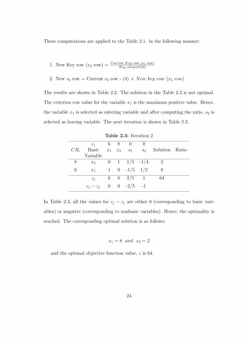
These computations are applied to the Table 2.1. in the following manner:
1. New Key row (x2 row) = Current Key row (s1 row)Key element(10)
2. New s2 row = Current s2 row - (4) × New key row (x2 row)
The results are shown in Table 2.2. The solution in the Table 2.2 is not optimal.
The criterion row value for the variable x1 is the maximum positive value. Hence,
the variable x1 is selected as entering variable and after computing the ratio, s2 is
selected as leaving variable. The next iteration is shown in Table 2.3.
Table 2.3: Iteration 2
cj 6 8 0 0CBi Basic x1 x2 s1 s2 Solution Ratio
Variable8 x2 0 1 1/5 -1/4 2
6 x1 1 0 -1/5 1/2 8
zj 6 8 2/5 1 64
cj − zj 0 0 -2/5 -1
In Table 2.3, all the values for cj − zj are either 0 (corresponding to basic vari-
ables) or negative (corresponding to nonbasic variables). Hence, the optimality is
reached. The corresponding optimal solution is as follows:
x1 = 8 and x2 = 2
and the optimal objective function value, z is 64.
24

2.2.4 Revised simplex method
The simplex method discussed in section 2.2 performs calculation on the entire
tableau during each iteration. However, updating all the elements in tableau dur-
ing a basis change is not really necessary for using the simplex method. The only
information needed in moving from one tableau (basic feasible solution) to another
tableau is as follows:
1. The relative profit coefficients (cj − zj row).
2. The column corresponding to the entering variable (Key column).
3. The current basic variables and their values (Solution column).
The information contained in other columns of the tableau plays no role in the
simplex process. Hence the solution of large linear programming problems on a
digital computer will become very inefficient and costly if the simplex method were
to be used in its full tableau form. However, revised simplex method is an improve-
ment over simplex method. The revised simplex method is computationally more
efficient and accurate. Its benefit is clearly comprehended in case of large LP
problems. The revised simplex method uses exactly the same steps as those in
simplex method but at each iteration the entire tableau is never calculated. The
relevant information it needs to move from one basic feasible solution to another
is directly generated from the original equations. The steps of the revised simplex
method (using matrix manipulations) can be summarized as follows:
Step 1. Obtain the initial feasible basis B. Determine the corresponding feasible
solution xB = B−1b.
25

Step 2. Obtain the corresponding simplex multipliers π = cBB−1. Check the
optimality of the current basic feasible solution (BFS). If the current basis
is optimal, then STOP.
Step 3. If the current BFS is not optimal, identify the entering variable xj (that
is, cj − zj = cj −∑m
i=1 πjaij = cj − πPj < 0).
Step 4. Obtain the column P̄j = B−1Pj and perform the minimum ratio test to
determine the leaving variable xl.
Step 5. Update the basis B (or B−1) and go to Step 2.
For more information and details, refer to [55].
26

2.3 Duality Theory and Its Applications
From both the theoretical and practical point of view, the theory of duality is one
of the most important and interesting concepts in linear programming. The basic
idea behind the duality theory is that every linear programming problem has an
associated linear programming called its dual such that a solution to the original
linear program also gives a solution to its dual. Thus, whenever a linear program
is solved by the simplex method, we are actually getting solutions for two linear
programming problems. The Dual can be considered as the “inverse” of the Primal
in every respect. The column coefficients in the Primal constrains become the
row co-efficients in the Dual constraints. The coefficients in the Primal objective
function become the right hand side constraints in the Dual constraints. The
column of constants on the right hand side of the Primal constraints becomes the
row of coefficients of the dual objective function. The direction of the inequalities
are reversed. If the primal objective function is a “Maximization” function then the
dual objective function is a “Minimization” function and vice-versa. The concept of
duality is very much in useful to obtain additional information about the variation
in the optimal solution when certain changes are effected in the constraint co-
efficient, resource availabilities and objective function co-efficients. This is termed
as “post optimality” or “sensitivity analysis”.
27

The concept of a dual is introduced by the following programme.
Example 2.1
Maximze Z = x1 + 2x2 - 3x3 + 4x4
subject tox1 + 2x2 + 2x3 - 3x4 ≤ 25,2x1 + x2 - 3x3 + 2x4 ≤ 15,x1 , x2 , x3 , x4 ≥ 0.
The above linear programme has two constraints and four variables. The dual
of this problem is written as
Minimize W = 25y1 + 15y2
subject toy1 + 2y2 ≥ 1,2y1 + y2 ≥ 2,2y1 - 3y2 ≥ -3,−3y1 + 2y2 ≥ 4,y1 , y2 ≥ 0.
y1 and y2 are called the dual variables. The original problem is called the primal
problem. Comparing the primal and the dual problems, we observe the following
relationships:
1. The objective function coefficients of the primal objective function have be-
come the right-hand-side constants of dual. Similarly, the right-hand-side
constants of primal problem have become the objective function coefficients
of the dual.
2. The inequalities have been reversed in the constraints.
3. The objective is changed from maximization in primal to minimization in
dual.
28

4. Each column in the primal corresponds to a constraint (row) in the dual.
Thus, the number of dual constraints is equal to the number of primal vari-
ables.
5. Each constraint(row) in the primal corresponds to a column in the dual.
Hence, there is one dual variable for every primal constraint.
6. The dual of the dual is the primal problem.
In both of the primal and the dual problems, the variables are nonnegative and
the constraints are inequalities. Such problems are called symmetric dual linear
programmes.
Definition. A linear programme is said to be in symmetric form, if all the
variables are restricted to be nonnegative, and all the constraints are inequalities
(in a maximization problem the inequalities must be in “less than or equal to”
form and in a minimization problem they must be in “greater than or equal to”).
In matrix notation the symmetric dual linear programmes are:
Primal:
Maximize Z = C ′Xsubject to
AX ≤ b,X ≥ 0.
Dual:
Minimize W = b′Ysubject to
A′Y ≥ C,Y ≥ 0.
29

Where A is an m×n matrix, b is an m× 1 column vector, C is a n× 1 column
vector, X is an n× 1 column vector and Y is an m× 1 column vector.
Te following table describes more general relations between the primal and dual
that can be easily derived from the symmetric form definition. They relate the
sense of constraint i in the primal with the sign restriction for yi in the dual, and
sign restriction of xj in the primal with the sense of constraint j in the dual. Note
that when these alternative definitions are allowed there are many ways to write
the primal and dual problems; however, they are all equivalent.
Modifications in the primal-dual formulations
Primal model Dual modelMaximization Minimization
Constraint i is ≤ yi ≥ 0Constraint i is = yi is unrestrictedConstraint i is ≥ yi ≤ 0
xj ≥ 0 Constraint j is ≥xj is unrestricted Constraint j is =
xj ≤ 0 Constraint j is ≤
2.3.1 Economic interpretation of the dual problem
Primal:
Consider a manufacturer who makes n products out of m resources. To make
one unit of product j it takes aij units of resource i. The manufacturer has obtained
bi units of resources i in hand, and the unit price of product j is cj. Therefore, the
primal problem leads the manufacturer to find an optimal production plan that
maximizes the sales with available resources.
30

Dual:
Lets assume the manufacturer gets the resources from a supplier. The man-
ufacturer wants to negotiate the unit purchasing price yi for resource i with the
supplier. Therefore, the manufacturers objective is to minimize the total purchas-
ing price b′Y in obtaining the resources bi. Since the market price cj and the
“product-resource” conversion ratio aij are open information on market, the man-
ufacturer knows that, at least, a “smart” supplier would like to charge him as much
as possible, so that
a1jy1 + a2jy2 + · · ·+ amjym ≥ cj.
In this way, the dual linear program leads the manufacturer to come up with
a least-cost plan in which the purchasing prices are acceptable to the “smart”
supplier.
An example is giving to get more understanding on above economic interpre-
tation. Let n = 3 (products are Desk, Table and Chair) and m = 3 (resources
are Lumber, Finishing hours(needed time) and Carpentry hours). The amount of
each resource which is needed to make one unit of certain type of furniture is as
follows:
XXXXXXXXXXXXResourceProduct
Desk Table Chair
Lumber 4 lft 6 lft 1 lftFinishing hours 4 hrs 2 hrs 1.5 hrsCarpentry hours 2 hrs 1.5 hrs 0.5 hrs
48 lft of lumber, 20 hours of finishing hours and 4 carpentry hours are available.
A desk sells for $60, a table for $30 and a chair for $20. How many of each type
furniture should manufacturer produce?
Let x1, x2, and x3 respectively denote the number of desks, tables and chairs
31

produced. This problem is solved with the following LP:
Maximize Z = 60x1 + 30x2 + 20x3
subject to8x1 + 6x2 + x3 ≤ 48,4x1 + 2x2 + 1.5x3 ≤ 20,2x1 + 1.5x2 + 0.5x3 ≤ 8,x1 , x2 , x3 ≥ 0.
Suppose that an investor wants to buy the resources. What are the fair prices,
y1, y2, y3, that the investor should pay for a lft of lumber, one hour of finishing
and one hour of carpentry?
The investor wants to minimize buying cost. Then, his objective can be written as
min W = 48y1 + 20y2 + 8y3
In exchange for the resources that could make one desk, the investor is offering
(8y1 + 4y2 + 3y3) dollars. This amount should be larger than what manufacturer
could make out of manufacturing one desk ($60). Therefore,
8y1 + 4y2 + 2y3 ≥ 60
Similarly, by considering the “fair” amounts that the investor should pay for the
combination of resources that are required to make one table and one chair, we
conclude
6y1 + 2y2 + 1.5y3 ≥ 30
y1 + 1.5y2 + 0.5y3 ≥ 20
32

Consequently, the investor should pay the prices y1, y2, y3, solution to the
following LP:
Minimize W = 48y1 + 20y2 + 8y3
subject to8y1 + 4y2 + 2y3 ≥ 60,6y1 + 2y2 + 1.5y3 ≥ 30,y1 + 1.5y2 + 0.5y3 ≥ 20,y1 , y2 , y3 ≥ 0.
The above LP is the dual to the manufacturers LP. The dual variables are often
referred to as shadow prices, the fair market prices, or the dual prices.
Now, we shall turn our attention to some of the duality theorems that gives
important relationships between the primal and the dual solution.
Theorem 2.1: Weak Duality Theorem
Consider the symmetric primal-dual linear programmes,Max Z = C ′X, s. t. AX ≤
b, X ≥ 0, and Min W = b′Y, s. t. A′X ≥ C, Y ≥ 0. The value of the objective
function of the minimum problem (dual) for any feasible solution is always greater
than or equal to that of the maximum problem (primal).
From the weak duality theorem we can infer the following important results:
Corollary 2.1 The value of the objective function of the maximum (primal)
problem for any (primal) feasible solution is a lower bound to the minimum
value of the dual objective.
Corollary 2.2 Similarly the objective function value of the minimum problem
(dual) for any (dual) feasible solution is an upper bound to the maximum
value of the primal objective.
33

Corollary 2.3 If the primal problem is feasible and its objective is unbounded
(i.e., max Z → +∞), then the dual problem is infeasible.
Corollary 2.4 Similarly, if the dual problem is feasible, and is unbounded (i.e.,minW →
−∞), then the primal problem is infeasible.
Theorem 2.2: Optimality Criterion Theorem
If there exist feasible solutions X0 and Y 0 for the symmetric dual linear pra-
grammes such that the corresponding values of their objective functions are equal,
then these feasible solution are in fact optimal solutions to their respective prob-
lems.
Theorem 2.3: Main Duality Theorem
If both the primal and dual problems are feasible, then they both have optimal
solutions such their optimal values of the objective functions are equal.
We will use the properties of duality theory in proposed search algorithm, see
section 5.
34

2.4 Computational Problems in Simplex Method
There are a number of computational problems that may arise during the actual
application of the simplex method for solving a linear programming problem. In
this section we discuss some complication that may occur.
1. Ties in the selection of the nonbasic variable:
In a maximization problem, the nonbasic variable with the largest positive
value in the cj−zj row is chosen. In case there exists more than one variable
with the same largest positive value in the cj− zj row, then we have a tie for
selecting the nonbasic variable.
2. Ties in the minimum ratio rule and degeneracy:
While applying the minimum ratio rule it is possible for two or more con-
straints to give the same least ratio value. This result in a tie for selecting
which basic variable should leave the basis. This complication causes degen-
eracy in basic feasible solution.
Degenerate basic feasible solution: A basic feasible solution is said to
be degenerate basic feasible solution if at least one basic variable in the so-
lution equals zero.
3. Cycling:
At a degenerate basic solution, there is a risk of getting trapped in a cycle.
When there exist degeneracy in feasible solution we can’t say that simplex
method will be terminated in a finite number of iterations, because this phe-
nomenon causes that we obtain a new basic feasible solution in the next
iteration which has no effect on the objective function value. It is then the-
35

oretically possible to select a sequence of admissible bases that is repeatedly
selected without over satisfying the optimality criteria and, hence, never
reaches a optimal solution. A number of anticycling procedure have been
developed [17, 14, 66, 49, 10]. These anticycling method are not used in
practice partly because they would slow the computer program down and
partly because of the difficulty of recognizing a true zero numerically [7].
2.4.1 Complexity of the simplex method
The simplex method is not a good computational algorithm. It may lead to an
exponential number of iteration as the example which is provided by Klee and
Minty (1972). They showed that the simplex method as formulated by Dantzig
visit all 2n vertices before arriving at the optimal vertex, this shows that the worst
case complexity of the simplex algorithm is exponential time. Also, the number
of arithmetic operations in the algorithm grows exponentially with the number of
variables. The first polynomial time (interior point) algorithms, Ellipsoid method,
for linear programming were given by Khachian (1979), then Karmarkar (1984)
suggested the second polynomial time algorithm. Unlike the ellipsoid method
Karmarkar’s method solves the very larg linear programming problems faster than
does the simplex method [58]. Both the ellipsoid method and the karmarkar’s
method are mathematically iterative and they are not better than simplex algo-
rithm certainly for small linear programming problems and possibly for reasonably
large linear programming problems [58].
According this restrictions of simplex algorithm and interior point methods pro-
vided by Khachian (1979) and Karmarkar (1984) and their variants, we need a
new algorithm. We are going to give a stochastic search algorithm to obtain a
near-optimal solution. Stochastic search algorithm are useful for applications
36

where stable and acceptable (i. e. near-optimal) answers are desired quickly [27].
In general, Stochastic search algorithms do not require knowledge of a derivative
(as in gradient search methods) and perform best with highly nonlinear or highly
combinatorial problems [12].
37

2.5 Proposed Stochastic Search Algorithm
Consider the linear programming problem in the canonical form:
P: max z = c1x1 + c2x2 + . . . + cnxnsubject to
a11x1 + a12x2 + . . . + a1nxn ≤ b1,a21x1 + a22x2 + . . . + a2nxn ≤ b2,
......
......
...am1x1 + am2x2 + . . . + amnxn ≤ bm,x1 , x2 , . . . , xn ≥ 0.
Consider the decision variable xj for some j = 1, 2, . . . , n. If all other decision
variables are set to zero, then xj must satisfy aijxj ≤ bi, i = 1, 2, . . . ,m. To satisfy
all of this condition for all i, we must have
0 ≤ xj ≤ min{i: aij>0}
{biaij
}, 1 ≤ j ≤ n.
The bounding box B ={x| 0 ≤ xj ≤ min{i: aij>0}
{biaij
}, 1 ≤ j ≤ n
}, B ⊂ En,
contains the simplex set of feasible solutions of P . All feasible solutions of P are
elements of B, though the converse may not hold. In this case all dual decision
variables have zero lower bound, in fact, the positive quadrant contains the simplex
representing the set of feasible solution of dual problem. We call it DB.
Now, generate a random element each from B and DB using a specified dis-
tribution, pr, on B and DB. If this element is primal feasible, then compute the
primal objective function at this solution. Ignore all infeasible elements. Compute
the largest value of the primal objective functions for these primal feasible solu-
tions. The same process is applied to the dual problem by computing the smallest
value of dual objective functions for the generated feasible dual solutions. In this
process, a feasible primal solution is declared inadmissible if the value of the primal
objective function does not exceed the highest value obtained till then. A feasible
38

dual solution is declared inadmissible if the value of the dual objective function is
not smaller than the smallest value obtained till then. We keep track of the num-
ber of generated elements, the number of feasible solutions among these and the
number of admissible points among the latter, in both problems. The procedure
can be terminated after generating a specified number of
1. random elements
2. feasible solutions, or
3. admissible solutions.
The best solution at termination of the procedure is declared as the near-
optimal solution. A second possible termination rule is obtained by considering the
gap between near optimal primal and near optimal dual solutions. The procedure
is terminated when this gap (or interval) is sufficiently small.
2.5.1 Multiple starts
The simulation approach obtains a near-optimal solution for every starting value.
Near-optimality of the final solution does not depend on the initial value and hence
the rate of convergence can not be determined. Therefore, it may be convenient
to begin with more than one initial value, generating an independent sequence of
solutions for every initial value. This will give us several end-points and the best
of these will be better than the solution obtained from any one of them.
The maximum of the primal objective function and the minimum of the dual
objective function obtained through the above procedure are both near-optimal.
This method is not iterative in the sense that consecutive solutions may not im-
prove the objective function. Also, it is simple from the mathematical point of
view and there are no complicated computations.
39

Algorithmically, the method is described as follows.
• Initialization in primal problem (PP):
Set i = 1, zn−o = 0, xn−o = 0, io = 100 (number of feasible points).
1. Generation in PP:
Step 1.1. Generate xi ∈ B using uniform distribution on the bounding
box B.
Step 1. 2. Test feasibility of xi.
Step 1.3. If xi is feasible, go to step 1.4. Otherwise, go to step 1.1.
2. Computation in PP:
Step 1.4. Compute zi = c′xi, i = 1, 2, · · · , io.
Step 1.5. zn−o = maxi(zi), i = 1, 2, · · · , io and xn−o = associated xi
with zn−o.
3. Termination in PP:
Step 1.6. Keep the values of xn−o, zn−o and stop.
• Initialization in dual problem (DP):
Set j = 1, gn−o is infinity, yn−o is infinity, jo = 100 (number of feasible
points).
1. Generation in DP:
Step 2.1. Generate yj∈ DB using uniform distribution on the bound-
ing box DB.
Step 2.2. Test feasibility of yj.
Step 2.3. If yj
is feasible, go to step 2.4. Otherwise, go to step 2.1.
40

2. Computation in DP:
Step 2.4. Compute gj = b′yj, j = 1, 2, · · · , jo.
Step 2.5. gn−o = minj(gj), j = 1, 2, · · · , jo and gn−o = associated yj
with gn−o.
3. Termination in DP:
Step 2.6. Keep the values of yn−o, gn−o and stop.
• Termination in restarting: if (gn−o − zn−o) ≤ ε, small positive value, or
the number of restarting get equal to its initial value, then output the values
of zn−o, xn−o, gn−o, yn−o and stop restart.
2.5.2 Choice of probability distribution (pr)
For the probability distribution, we have two choices.
1. Uniform distribution.
In this case, every element is generated from B and DB with equal prob-
ability of selection. A significant limitation of uniform distribution is the
progressively increasing rejection rate (rejection can occur for one of the two
reasons: infeasibility and inadmissibility). This happens because points are
generated with equal probability and rejection depends on the position of
the current solution.
2. Non-Uniform distributions.
Due to the limitation of Uniform distribution, we propose to use a non-
uniform distribution. As a pilot study, we use the normal distribution with
mean µj = upper bound of xj, j = 1, · · · , n in PP and νi = lower bound of
41

yi, i = 1, · · · ,m in DP and unit variances. The results of pilot study show
that the normal distribution is more suitable than uniform distribution.
A major limitation of the normal distribution is that half of the generated
points are expected to exceed the mean. This implies a rejection rate ex-
ceeding 1/2. This can be overcome by modifying the mean as follows.
We take a fraction f ∈ (0, 1) and use the mean
f · µj, 1 ≤ j ≤ n or f · νi, 1 ≤ i ≤ m.
We tried some fractions to identify a good value for the fraction.
Another feature of the normal distribution is its unbounded support. Since
the set of feasible primal solutions is bounded, we considered a distribution on
a bounded support. In particular, we tried the multivariate Beta distribution,
with the marginal distribution of xj on[0, min{i: aij>0}
{biaij
: 1 ≤ j ≤ n}]
with parameters α, β > 0 so that α > β or α = k · β with k > 1.
The gamma distribution is reasonable for the dual problem because its fea-
sible solution set is unbounded.
For a problem having integer optimal solution, a discrete probability distri-
bution is found to be very efficient. This is more so if the coordinates of
bounding points are small multiples of optimal xj or yi.
42

2.6 Results of Simulation Studies
We consider some examples and implement the proposed simulation algorithm
under some non-uniform distributions, namely normal, beta, Weibull and gamma,
with different parameters and two discrete distributions, namely geometric and
Poisson.
The following symbols are used in the tables.
• Zn−o and gn−o are the primal and dual near-optimal objective functions,respectively.
• gap is the length of interval between primal and dual near-optimal values
(gap).
• CPU time/Sec. is the average of running time of stochastic algorithm in
terms of second per restart.
1. Beale’s Example
The following example is called Beale’s example and falls into cycling when
the simplex algorithm is used. The optimum value of objective function is
0.05.
max z = 0.75x1 − 150x2 + 0.02x3 − 6x4
s.t.
0.25x1 − 60x2 − 0.04x3 + 9x4 ≤ 0,
0.5x1 − 90x2 − 0.02x3 + 3x4 ≤ 0,
x3 ≤ 1,
x1, x2, x3, x4 ≥ 0.
43
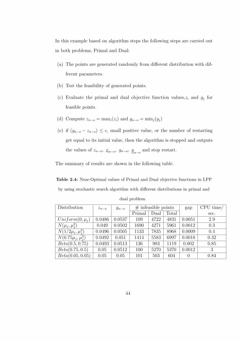
In this example based on algorithm steps the following steps are carried out
in both problems, Primal and Dual:
(a) The points are generated randomly from different distribution with dif-
ferent parameters.
(b) Test the feasibility of generated points.
(c) Evaluate the primal and dual objective function values,zi and gj for
feasible points.
(d) Compute zn−o = maxi(zi) and gn−o = minj(gj)
(e) if (gn−o − zn−o) ≤ ε, small positive value, or the number of restarting
get equal to its initial value, then the algorithm is stopped and outputs
the values of zn−o, xn−o, gn−o, yn−o and stop restart.
The summary of results are shown in the following table.
Table 2.4: Near-Optimal values of Primal and Dual objective functions in LPP
by using stochastic search algorithm with different distributions in primal and
dual problem.
Distribution zn−o gn−o # infeasible points gap CPU time/Primal Dual Total sec.
Uniform(0, µj) 0.0486 0.0537 109 4722 4831 0.0051 2.9N(µj, µ
2j) 0.049 0.0502 1690 4271 5961 0.0012 0.3
N(1/2µj, µ2j) 0.0496 0.0505 1133 7835 8968 0.0009 0.4
N(0.75µj, µ2j) 0.0492 0.051 1414 5583 6997 0.0018 0.32
Beta(0.5, 0.75) 0.0493 0.0513 136 983 1119 0.002 0.85Beta(0.75, 0.5) 0.05 0.0512 100 5270 5370 0.0012 3Beta(0.05, 0.05) 0.05 0.05 101 503 604 0 0.84
44

• As we mentioned before, the performance of non-uniform statistical dis-
tributions is better than uniform distribution. This can be understood
from running time of proposed algorithm and gap (distance between
primal and dual near-optimal objective function values).
• When normal distribution with the mean at the half of upper (lower)
bound for primal (dual) decision variable is considered the length of
gap is smaller than other cases of mean, this means the primal and dual
near-optimal value are nearer to each other than other cases of mean.
• The results which have obtained from Beta distribution with parameters
0 < α, β < 1 are better than other cases of α, β.
2. Kuhn’s Example
This example faces to cycling by using simplex algorithm. The optimum
value of objective function is 2.
max z = 2x1 + 3x2 − x3 − 12x4
s.t.
−2x1 − 9x2 + x3 + 9x4 ≤ 0,
1
3x1 + x2 −
1
3x3 − 2x4 ≤ 0,
2x1 + 3x2 − x3 − 12x4 ≤ 2,
x1, x2, x3, x4 ≥ 0.
In this example based on algorithm steps the following steps are carried out
in both problems, Primal and Dual:
(a) The points are generated randomly from different distribution with dif-
ferent parameters.
45

(b) Test the feasibility of generated points.
(c) Evaluate the primal and dual objective function values,zi and gj for
feasible points.
(d) Compute zn−o = maxi(zi) and gn−o = minj(gj)
(e) if (gn−o − zn−o) ≤ ε, small positive value, or the number of restarting
get equal to its initial value, then the algorithm is stopped and outputs
the values of zn−o, xn−o, gn−o, yn−o and stop restart.
The summary of results are shown in the following table.
Table 2.5: Near-Optimal values of Primal and Dual objective functions in LPP
by using stochastic search algorithm with different distributions in primal and
dual problem.
Distribution zn−o gn−o # infeasible points gap CPU time/Primal Dual Total sec.
Uniform(0, µj) 1.9993 2 290 1491 1781 0.000071 0.29N(µj, 1) 1.9988 2 413 1595 2008 0.0012 0.124N(µj, µ
2j) 1.9989 2 709 1536 2245 0.0011 0.117
N(1/2µj, µ2j) 1.9988 2 1620 1573 3193 0.0012 0.125
Beta(0.5, 0.75) 1.9984 2 354 1510 1861 0.0016 0.238Beta(0.5, 0.5) 1.9954 2 269 1310 1519 0.0046 0.223Gamma(1, 1) 1.9947 2 385 1794 2179 0.0053 0.161Gamma(1, 2) 1.9995 2 426 1426 1852 0.00005 0.1605Geo(0.5) 2 2 431 1676 2107 0 0.221
• For this example uniform and non-uniform distributions with consider-
ing a discrete distribution (Geometric(p = 0.5)) for dual problem have
good and almost same performance.
• The problem has an integer optimal solution then, a discrete distribution
(Geometric(p = 0.5))without considering the upper bounds of decision
46
variables in primal problem was applied and the exact optimal solution
for both problems obtained.
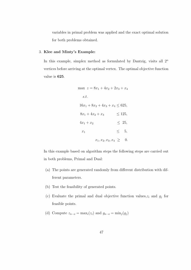
3. Klee and Minty’s Example:
In this example, simplex method as formulated by Dantzig, visits all 2n
vertices before arriving at the optimal vertex. The optimal objective function
value is 625.
max z = 8x1 + 4x2 + 2x3 + x4
s.t.
16x1 + 8x2 + 4x3 + x4 ≤ 625,
8x1 + 4x2 + x3 ≤ 125,
4x1 + x2 ≤ 25,
x1 ≤ 5,
x1, x2, x3, x4 ≥ 0.
In this example based on algorithm steps the following steps are carried out
in both problems, Primal and Dual:
(a) The points are generated randomly from different distribution with dif-
ferent parameters.
(b) Test the feasibility of generated points.
(c) Evaluate the primal and dual objective function values,zi and gj for
feasible points.
(d) Compute zn−o = maxi(zi) and gn−o = minj(gj)
47

(e) if (gn−o − zn−o) ≤ ε, small positive value, or the number of restarting
get equal to its initial value, then the algorithm is stopped and outputs
the values of zn−o, xn−o, gn−o, yn−o and stop restart.
The summary of results are shown in the following table.
Table 2.6: Near-Optimal values of Primal and Dual objective functions in LPP
by using stochastic search algorithm with different distributions in primal and
dual problem.
Distribution zn−o gn−o # infeasible points gap time/Primal Dual Total sec.
Uniform(0, µj) 588.05 634.05 20254 0 20254 46 14.19N(µj, µ
2j) na na na na na na na
N(1/2µj, µ2j) 570.3 625.1 64880 237 65117 54.8 1.35
Beta(0.5, 0.75) 614.03 627.69 1920 0 1920 13.66 1.64Beta(0.5, 1) 618.08 626.22 1179 0 1179 8.14 1.04Beta(0.25, 1) 623.31 625.01 171 0 171 1.7 0.47Beta(0.25, 0.75) 624.35 625.03 322 0 322 0.68 0.55Beta(0.05, 0.05) 625 625 1121 0 1121 0 1.33Geo(0.5) 625 625 833 0 833 0 0.55
• Also in this example, the efficiency of most of non-uniform statistical dis-
tributions is better than uniform distribution. This can be understood
from running time of proposed algorithm and gap (distance between
primal and dual near-optimal objective function values).
• The normal distribution with the mean at upper (lower) bound for pri-
mal (dual) decision variable is not applicable. But normal distribution
with mean at the half of the upper (lower) bound for primal (dual)
decision variable has better performance than uniform distribution.
• The results which are obtained from Beta distribution with parameters
0 < α < 1 and β = 1 are better than other cases of α, β.
48

• The coordinates of bounding points of this example are multiples of
optimal solution xopt, yopt then a discreet distribution is very efficient
and here the Geometric distribution with parameter p = 0.5 reaches to
the exact optimal solution which is integer.
4. Further example
This example has integer optimal solution in both problems and the optimal
objective function value is 2200.
max z = 45x1 + 80x2
s.t.
5x1 + 20x2 ≤ 400,
10x1 + 15x2 ≤ 450,
x1, x2 ≥ 0.
In this example based on algorithm steps the following steps are carried out
in both problems, Primal and Dual:
(a) The points are generated randomly from different distribution with dif-
ferent parameters.
(b) Test the feasibility of generated points.
(c) Evaluate the primal and dual objective function values,zi and gj for
feasible points.
(d) Compute zn−o = maxi(zi) and gn−o = minj(gj)
(e) if (gn−o − zn−o) ≤ ε, small positive value, or the number of restarting
get equal to its initial value, then the algorithm is stopped and outputs
the values of zn−o, xn−o, gn−o, yn−o and stop restart.
49

The summary of results are shown in the following table.
Table 2.7: Near-Optimal values of Primal and Dual objective functions in LPP
by using stochastic search algorithm with different distributions in primal and
dual problem.
Distribution zn−o gn−o # infeasible points gap CPU time/Primal Dual Total sec.
N(µj, µ2j) 2189.8 2208.32 1335 350 1685 18.472 0.076
N(1/2µj, µ2j) 2191.6 2207.2 1082 346 1428 15.536 0.071
Weibull(µj, 3.5) 2198.7 2206.9 1454 550 2004 8.25 0.136Poisson(µj) 2200 2200 50000 2070 52070 0 18.2Poisson(1/2µj) 2200 2200 17 1675 1692 0 0.191
The Uniform distribution has no efficiency for this example. Then, we applied
Non-uniform distribution for both primal and dual problems. Normal and Weibull
distributions for primal and Gamma distribution for dual problem. As it can be
seen when a fraction of mean parameter of Normal distribution is considered the
efficiency of algorithm is increased. It is clear that the Weibull distribution for scale
parameters bigger than 3.4 leads to Normal distribution and we see the behavior of
this distribution. Because of existence an integer solution for the problem, discrete
distributions are best for this problem.
All this work has been published in the Pakistan Journal of Statistics, Vol. 27,
No. 1, pp. 65-74.
50

2.7 Conclusions
1. Since stochastic search technique uses pseudo-random numbers, there is no
learning in the simulation based algorithm. As a result, more work does not
necessarily imply improvement in the solution. On the other hand, the result
is not necessarily bad if we have not worked much. Hence, an early solution
can be a near-optimal solution and may not significantly improve with more
work.
2. Generating feasible solutions is the major work in this algorithm. The bound-
ing box is either a hyper-cube or cuboid and then there is a high rejection
rate, or the complete Euclidean space with the same consequence. Attempts
are being made to improve the performance of random solution generator.
3. Stochastic search algorithm is not an iterative procedure.
4. Stochastic search algorithm is simple from mathematical point of view and
there are no complicated computations.
5. Stopping rule can be based on number feasible points in generation, num-
ber restarts the algorithm, length of interval of optimal objective function
value (the length of gap between primal near-optimal and dual near-optimal
values).
6. Discrete distributions like Geometric and Poisson are very efficient in certain
special cases.
51
Recommended