July 15, 2008 20:33 World Scientific Review Volume - 9in x 6in wdijkstra
Chapter 1
Condition numbers and local errors in the boundary
element method
W. Dijkstra∗, G. Kakuba and R. M. M. Mattheij
Eindhoven University of Technology, Department of Mathematics andComputing Science, P.O. Box 513, 5600 MB Eindhoven, The Netherlands,
In this chapter we investigate local errors and condition numbers in theBEM. The results of these investigations are important in guiding adap-tive meshing strategies and solvability of linear systems in BEM. Weshow that the local error for the BEM with constant or linear elementsdecreases quadratically with the boundary element mesh size. We alsoinvestigate better ways of treating boundary conditions to reduce thelocal errors. The results of our numerical experiments confirm the the-ory. The values of the condition numbers of the matrices that appear inthe BEM depend on the shape and size of the domain on which a prob-lem is defined. For certain critical domains these condition numberscan even become infinitely large. We show that this holds for severalclasses of boundary value problems and propose a number of strategiesto guarantee moderate condition numbers.
1.1. Introduction
The subject of errors in the boundary element method (BEM) is still a
very interesting one and some aspects have not yet been as explored as
they are in other numerical methods like FEM and FDM. Errors in BEM
solutions may be due to discretisation or to inaccuracies in the solver that
involves the use of BEM matrices with high condition numbers. For a
given discretisation there are several ways to implement BEM because of
the choice in collocation and nodal points. These will all influence the
resulting error in the solution. In most cases where error measurement has
been performed, like in adaptive refinement, the main focus has been a
measure of the error rather than a fundamental analysis of the error and∗Mecal, P.O. Box 375, 5500 AJ Veldhoven, The Netherlands
1
July 15, 2008 20:33 World Scientific Review Volume - 9in x 6in wdijkstra
2 W. Dijkstra, G. Kakuba and R. M. M. Mattheij
its behaviour. This chapter presents recent results on such fundamental
analysis on local errors in BEM solutions. The results presented will not
only be helpful in choosing an implementation strategy but also in guiding
adaptive refinement techniques.
Several techniques have been used to measure BEM errors in the area
of adaptive refinement. For instance the discretisation error is estimated
by the difference between two solutions obtained using different collocation
points but the same discretisation.1 Another technique uses the first (sin-
gular integral equation) and the second (hypersingular integral equation)
kind formulations to provide an error estimate.2 Data from the first kind
of equation is substituted into the second kind to obtain a residual which
is then used to estimate the error. Some authors have used a posteriori
error estimation in FEM as a guiding tool to develop error estimates for
BEM.3 Unfortunately usually such techniques are restricted to Galerkin
BEM. In our case we would like to start from the basics of the boundary
integral equation (BIE) discretisation to develop error analyses for colloca-
tion BEM for potential problems. Though the ideas could easily be adapted
to 3D, we will discuss 2D problems and the Laplace equation in particular.
It is well-known that the Laplace equation in differential form with
either Dirichlet or mixed boundary conditions has a unique solution. How-
ever, when the Laplace equation is transformed to a BIE it is not straight-
forward that this carries over to the BIE. It is noted that the BIE for the
Dirichlet Laplace equation does not always have a unique solution.4–7 Cer-
tain domains can be distinguished on which the BIE becomes singular and a
non-trivial solution of the homogeneous equations can be found. A multiple
of this solution can be added to the solution of the non-homogeneous equa-
tions, which is then no longer unique. For each domain there exists exactly
one rescaled version of this domain for which the BIE becomes singular.
This introduces an extraordinary phenomenon for the BIEs; uniqueness of
the solutions depends on the scale of the domain.
After discretisation of the boundary of the domain, the BIE transforms
into a linear system of equations. When the BIE is singular, one may
expect that the linear system is also singular, or at least ill-conditioned.
This is reflected by the condition number of the system matrix. If this
condition number is infinitely large, then the linear system is singular. As
a consequence, the linear system does not have a unique solution. If the
condition number is not infinitely large, but still large, the linear system
is ill-conditioned and difficult to solve. Hence the condition number also
greatly affects the local error in the BEM solution. Note that it is a matter
July 15, 2008 20:33 World Scientific Review Volume - 9in x 6in wdijkstra
Condition numbers and local errors in the boundary element method 3
of taste to decide what ‘large’ means in the context of condition numbers.
The domains on which the BIE does not have a unique solution are
related to the so called logarithmic capacity. The logarithmic capacity is
a real positive number being a function of the domain. This concept orig-
inates from the field of measure theory, but it also appears in potential
theory. The concept of a capacity applied to a single domain may be a bit
confusing, as usually the electrical capacity is defined as a charge differ-
ence between two conducting objects. The logarithmic capacity however is
related to a single domain.
In potential theory it is shown that when the logarithmic capacity of a
domain is equal to one, then the homogeneous BIE for the Dirichlet Laplace
equation on the boundary of that domain has a non-trivial solution.8–10
This allows us to a-priori detect whether a BIE will become singular on a
certain domain. Namely, we have to compute the logarithmic capacity and
verify whether it is equal to one. Additionally, the logarithmic capacity
also enables us to modify the BIE such that it does not become singular.
We can scale the domain in such a way that its logarithmic capacity is
not equal to one. The BIE on the corresponding boundary will then be
nonsingular.
The BIE for the Laplace equation with mixed boundary conditions did
not receive much attention until now.11 However, a similar phenomenon
as for the Dirichlet case takes place for mixed conditions. For each domain
there exists exactly one rescaled version of this domain for which the BIE
becomes singular. In this chapter we investigate both the BIE for the
Laplace equation with Dirichlet conditions and mixed conditions and the
related linear systems. We also extend the research to flow problems in
particular to BEM solutions of the Stokes equations.
This chapter is outlined as follows. Section 1.2 gives a recapitulation
of the BEM formulation. An outline of the integral equation formulation
for a Laplace problem and its discretisation is presented. In Section 1.3
we present a discussion on local errors in the BEM and give the theory
for the expected convergence rates of the local error for both constant and
linear elements. Numerical examples and results for a Dirichlet and mixed
problem are presented to illustrate the theory. Then a general insight into
the various ways to implement the BEM on a circle is presented.
In Section 1.4 we give a number of illustrative examples of BEM matrices
with large condition numbers. This motivates us to study the condition
numbers of BEM matrices in potential problems in Section 1.5. It is shown
that these condition numbers may become infinitely large under certain
July 15, 2008 20:33 World Scientific Review Volume - 9in x 6in wdijkstra
4 W. Dijkstra, G. Kakuba and R. M. M. Mattheij
conditions. This is also true for the condition numbers of BEM matrices in
flow problems, which is the topic of Section 1.6. The chapter is concluded
with a discussion on the results presented.
1.2. BEM formulation for potential problems
In this section we briefly present a BEM formulation. This we do here only
for potential problems but we will generalise it to Stokes equations as well
in a later section . The BEM is used to approximate solutions of boundary
value problems that can be formulated as integral equations. For the sake
of clarity, we consider potential problems governed by the Laplace equation
on a simply connected domain Ω in 2D with boundary Γ. That is
∇2u(r) = 0, r ∈ Ω. (1.1)
We will consider problems for which either the function u (Dirichlet) or its
outward normal derivative q := ∂u/∂n (Neumann) is given on Γ, or the
mixed problem where on one part of the boundary u is given and on the
other q is given. The integral equation formulation of (1.1) reads
cu+ Kdu = Ksq, r ∈ Γ (1.2)
Here Ks and Kd are the so called single and double layer operator, defined
as
(Ksq)(r) : =
∫
Γ
q(r′)G(r; r′)dΓr′ ,
(Kdu)(r) : =
∫
Γ
u(r′)∂
∂n′G(r; r′)dΓr′ . (1.3)
where r and r′ are points at the boundary and n′ is the unit outward
normal at r′ at Γ. The function G,
G(r; r′) :=1
2πlog
1
||r − r′||,
is the fundamental solution for the Laplace equation in 2D. The constant
c(r) = 12 if Γ is a smooth boundary at r. Thus (1.2) expresses the potential
at any point r in terms of its values u(r′) and the values of its outward
normal derivatives q(r′) on the boundary. Some of this information will
be given as boundary conditions and the rest has to be solved for. We
note that the most important step of BEM is to approximate the missing
boundary data as accurately as possible since the final step of computing
the unknown function in Ω is merely a case of postprocessing.
July 15, 2008 20:33 World Scientific Review Volume - 9in x 6in wdijkstra
Condition numbers and local errors in the boundary element method 5
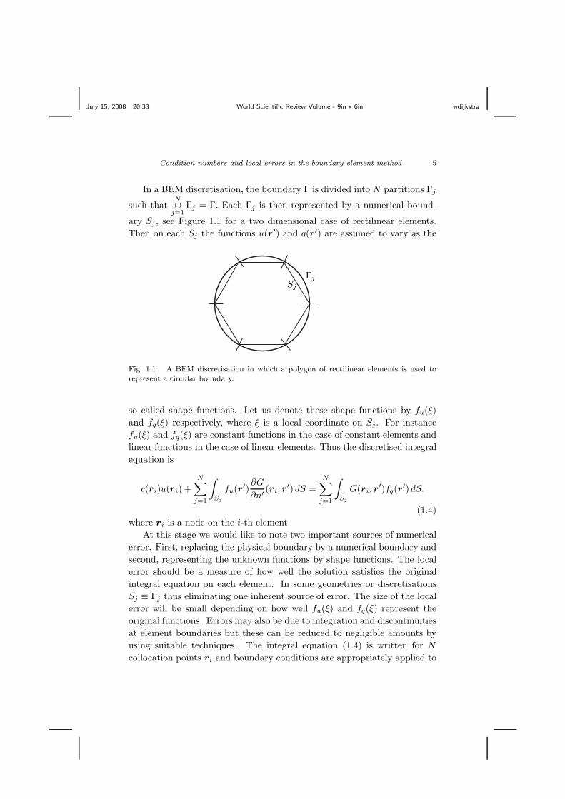
In a BEM discretisation, the boundary Γ is divided into N partitions Γj
such thatN∪
j=1Γj = Γ. Each Γj is then represented by a numerical bound-
ary Sj , see Figure 1.1 for a two dimensional case of rectilinear elements.
Then on each Sj the functions u(r′) and q(r′) are assumed to vary as the
Sj
Γj
Fig. 1.1. A BEM discretisation in which a polygon of rectilinear elements is used torepresent a circular boundary.
so called shape functions. Let us denote these shape functions by fu(ξ)
and fq(ξ) respectively, where ξ is a local coordinate on Sj . For instance
fu(ξ) and fq(ξ) are constant functions in the case of constant elements and
linear functions in the case of linear elements. Thus the discretised integral
equation is
c(ri)u(ri) +
N∑
j=1
∫
Sj
fu(r′)∂G
∂n′(ri; r
′) dS =
N∑
j=1
∫
Sj
G(ri; r′)fq(r
′) dS.
(1.4)
where ri is a node on the i-th element.
At this stage we would like to note two important sources of numerical
error. First, replacing the physical boundary by a numerical boundary and
second, representing the unknown functions by shape functions. The local
error should be a measure of how well the solution satisfies the original
integral equation on each element. In some geometries or discretisations
Sj ≡ Γj thus eliminating one inherent source of error. The size of the local
error will be small depending on how well fu(ξ) and fq(ξ) represent the
original functions. Errors may also be due to integration and discontinuities
at element boundaries but these can be reduced to negligible amounts by
using suitable techniques. The integral equation (1.4) is written for N
collocation points ri and boundary conditions are appropriately applied to
July 15, 2008 20:33 World Scientific Review Volume - 9in x 6in wdijkstra
6 W. Dijkstra, G. Kakuba and R. M. M. Mattheij
obtain a linear system of equations
Ax = b, (1.5)
where x is a vector of the unknown values of either u or q at the boundary.
1.3. Local errors in potential problems
Consider a Dirichlet problem given by,
∇2u(r) = 0, r ∈ Ω,
u(r) = g(r), r ∈ Γ.(1.6)
The unknown in this case is the outward normal derivative q(r′). Thus
what we want to solve for using BEM are the values of the normal flux
at the boundary Γ. That is, x = q = (q1 q2 · · · qN )T , a vector of the
unknown values of q(r′) at the boundary. Here we have introduced the
notation
u(r′i) =: ui and q(r′i) =: qi.
Let q := (q1 q2 · · · qN )T
be the corresponding BEM solution and let
q∗ := (q∗1 q∗2 · · · q∗N )
Tdenote the exact solution at the corresponding
nodes. The global error e is defined as
e := q∗ − q, (1.7)
that is, pointwise,
ej = q∗j − qj .
In order to advance our error investigations, let us define the exact values
of the integrals on the j-th element from source node i as
Iuij :=
∫
Γj
u(r′)∂G
∂n′(ri; r
′) dΓ, (1.8a)
Iqij :=
∫
Γj
G(ri; r′)q(r′) dΓ. (1.8b)
Let us also define the corresponding numerical estimates of (1.8) in the
BEM as
Iuij :=
∫
Sj
fu(r′)∂G
∂n′(ri; r
′) dS, (1.9a)
Iqij :=
∫
Sj
G(ri; r′)fq(r
′) dS. (1.9b)
July 15, 2008 20:33 World Scientific Review Volume - 9in x 6in wdijkstra
Condition numbers and local errors in the boundary element method 7
We then define the two contributions to the local error on element j due to
source node i as
dqij := Iq
ij − Iqij (1.10a)
duij := Iu
ij − Iuij (1.10b)
The total local error on element j due to source node i is
dij := dqij + du
ij . (1.11)
The cumulative local error for the i-th equation due to contributions from
all the elements is therefore given by
di := −N
∑
j=1
duij +
N∑
j=1
dqij . (1.12)
Consider the right hand side of the system (1.5); if we were to compute the
vector b exactly, then the i-th component would be
bEi := −ciu(r′i) −
N∑
j=1
∫
Γj
u(r′)∂G
∂n(r′i; r
′) dΓ.
The one we actually use in BEM is
bi = −ciu(r′i) −
N∑
j=1
∫
Sj
fu(r′)∂G
∂n(r′i; r
′) dS.
Let us define
δbi := bEi − bi = −N
∑
j=1
∫
Γj
∂G
∂n(ri; r
′)u(r′)dΓ
+
N∑
j=1
∫
Sj
fu(r′)∂G
∂n(r′i; r
′) dS = −N
∑
j=1
duij . (1.13)
The local error in (1.12) can therefore be expressed as
di = δbi +
N∑
j=1
dqij . (1.14)
If the right hand side is evaluated exactly, then δbi = 0 and the error (1.12)
would be
di =
N∑
j=1
dqij . (1.15)
July 15, 2008 20:33 World Scientific Review Volume - 9in x 6in wdijkstra
8 W. Dijkstra, G. Kakuba and R. M. M. Mattheij
In what follows we will asses further the behaviour of these local errors.
Theorem 1.1. The error in constant elements BEM is second order with
respect to grid size.
Proof. We need to show that the local error is third order in grid size.
Take the case of an element with a Dirichlet boundary condition where the
unknown is q(r′). Consider the integral (1.8b), that is
Iqij =
∫
Γj
G(ri; r′)q(r′) dΓ. (1.16)
Let lj be the length of Sj and ξ be a local coordinate on Sj such that
−lj/2 ≤ ξ ≤ lj/2.
Then (1.16) is transformed and evaluated in terms of ξ. Let ξj be the
midpoint of Sj . Suppose we have a Taylor series expansion of q(ξ) about
ξj , that is,
q(ξ) = q(ξj)+q′(ξj)(ξ−ξj)+
q′′(ξj)
2(ξ−ξj)
2+q(3)(ξj)
6(ξ−ξj)
3+· · · . (1.17)
Then, if we use (1.17) in (1.16), we have
2πIqij =
∫ lj/2
−lj/2
ln[r(ξ)]q(ξj) dξ +
∫ lj/2
−lj/2
ln[r(ξ)]q′(ξj)(ξ − ξj) dξ+
∫ lj/2
−lj/2
ln[r(ξ)]q′′(ξj)
2(ξ − ξj)
2 dξ + · · · , (1.18)
where
r(ξ) := ||ri − r′(ξ)||.
In constant elements BEM we only use the first term, that is,
Iqij ≈
1
2π
∫ lj/2
−lj/2
ln[r(ξ)]q(ξj ) dξ. (1.19)
So we have a truncation error whose principle term is the second term on
the right of (1.18). Let us consider the following integral of this term,
I2 :=
∫ lj/2
−lj/2
q′(ξj) ln[r(ξ)](ξ − ξj) dξ. (1.20)
We note that
r1 := r(ξ = −lj/2) ≤ r(ξ) ≤ r2 := r(ξ = lj/2). (1.21)
July 15, 2008 20:33 World Scientific Review Volume - 9in x 6in wdijkstra
Condition numbers and local errors in the boundary element method 9
We assume that ri is far enough such that r(ξ) remains nonzero. The
distance r(ξ) can be expanded about the point ξj as
r(ξ) = r(ξj) + r′(ξj)(ξ − ξj) + O((ξ − ξj)2) (1.22)
We introduce the definitions
ρ0 := r(ξj),
ρ1 : + r′(ξj).
so that we can write (1.22) as
r(ξ) = ρ0(1 +ρ1
ρ0(ξ − ξj) + O((ξ − ξj)
2).
Then
ln[r(ξ)] = ln(ρ0) +ρ1
ρ0(ξ − ξj) + O((ξ − ξj)
2).
The integral I2 can now be evaluated as
I2 =
∫ lj/2
−lj/2
ln[r(ξ)](ξ − ξj) dξ
=
∫ lj/2
−lj/2
ln(ρ0)(ξ − ξj) dξ
+
∫ lj/2
−lj/2
[ρ1
ρ0(ξ − ξj) + O((ξ − ξj)
2)](ξ − ξj) dξ. (1.23)
Since we use the midpoint as ξj , the first integral on the right of (1.23) is
zero so that we remain with
I2 =
∫ lj/2
−lj/2
ρ1
ρ0(ξ − ξj)
2 dξ + O((ξ − ξj)5). (1.24)
Then using the mean value theorem,
I2 ≈ρ1
ρ0(ζ − ξj)
2lj ζ ∈ (−lj/2, lj/2). (1.25)
For ξj a midpoint of Sj
|ζ − ξj | ≤ lj/2. (1.26)
Putting (1.25) and (1.26) together we have
|I2| ≤l3j4|ρ1/ρ0|.
which is third order in grid size. This shows that constant elements BEM
can be expected to be of second order.
July 15, 2008 20:33 World Scientific Review Volume - 9in x 6in wdijkstra
10 W. Dijkstra, G. Kakuba and R. M. M. Mattheij
Theorem 1.2. The error in linear elements BEM is second order with
respect to grid size.
Proof. Likewise we need to show that the local error is third order in grid
size. In linear elements the unknown function is assumed to vary linearly
on the element, that is,
q(ξ) ≈ p1(ξ) := α0 + α1ξ,
where α0 and α1 are constants and ξ a local coordinate on Sj . The error in
this case is due to the error when we interpolate by an order one polynomial
which is given by12
q(ξ) − p1(ξ) =q′′(η)
2(ξ − ξ0)(ξ − ξ1), η ∈ (ξ0, ξ1).
Using this result, the local error in BEM will be
Es1=
1
4π
∫ lj/2
−lj/2
ln[r(ξ)]q′′(η)(ξ − ξ0)(ξ − ξ1) dξ, (1.27)
where ξ0 and ξ1 are the interpolation coordinates. Again using the second
mean value theorem, we have
Es1≈
ln[r(β)]q′′(η)
4π
∫ lj/2
−lj/2
(ξ − ξ0)(ξ − ξ1) dξ
= −l3j
24πln[r(β)]q′′(η), (1.28)
where ξ0 = −lj/2, ξ1 = lj/2 and β an intermediate point. This result shows
that linear elements BEM can be expected to be of second order.
1.3.1. Numerical examples
In this section we will perform numerical experiments to illustrate the above
claims about the error. Results show that indeed we obtain second order
convergence of the error. Our experiments are performed on a circle which
rules out the errors caused by discontinuities at corners in other geometries
like a square. It would be a natural choice to work on a unit circle but
in our examples we avoid this choice for reasons that will become clear in
later sections.
Example 1.3.1. Consider the boundary value problem
∇2u(r) = 0, r ∈ Ω := r ∈ R2 : ||r|| ≤ 1.2,
u(r) = g(r′), r ∈ Γ.(1.29)
July 15, 2008 20:33 World Scientific Review Volume - 9in x 6in wdijkstra
Condition numbers and local errors in the boundary element method 11
The boundary condition function g(r′) is chosen such that the exact solu-
tion is
q(r′) =(r′ − rs) · n(r′)
||r′ − rs||2(1.30)
where the source point rs = (0.36, 1.8) is a fixed point outside Ω and n(r′)
is the outward normal at r′.
We will use this example to verify the results of theorems 1.1 and 1.2. Since
we have the analytic expression for the unknown q(r′) we can compute the
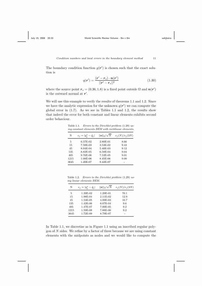
global error in (1.7). As we see in Tables 1.1 and 1.2, the results show
that indeed the error for both constant and linear elements exhibits second
order behaviour.
Table 1.1. Errors to the Dirichlet problem (1.29) us-ing constant elements BEM with rectilinear elements.
N ej = |q∗j − qj | ||e||2/√
N ej(N)/ej (3N)
5 6.57E-02 2.80E-01 8.6615 7.58E-03 3.53E-02 9.4345 8.04E-04 5.40E-03 9.12135 8.82E-05 6.58E-04 9.04405 9.76E-06 7.53E-05 9.011215 1.08E-06 8.45E-06 9.003645 1.20E-07 9.42E-07 -
Table 1.2. Errors to the Dirichlet problem (1.29) us-ing linear elements BEM.
N ej = |q∗j − qj | ||e||2/√
N ej(N)/ej(3N)
5 1.39E-02 1.29E-01 70.115 1.98E-04 2.11E-02 12.945 1.53E-05 4.89E-03 10.7135 1.42E-06 6.07E-04 9.6405 1.47E-07 7.00E-05 9.21215 1.59E-08 7.88E-06 9.23645 1.72E-09 8.79E-07 -
In Table 1.1, we discretise as in Figure 1.1 using an inscribed regular poly-
gon of N sides. We refine by a factor of three because we are using constant
elements with the midpoints as nodes and we would like to compute the
July 15, 2008 20:33 World Scientific Review Volume - 9in x 6in wdijkstra
12 W. Dijkstra, G. Kakuba and R. M. M. Mattheij
pointwise error as shown in the second column. For a better compari-
son, we use the same refinement factor for linear elements as well. Both
the pointwise error and the median 2-norm of the error show the same
trend of error convergence. The pointwise error is computed at the point
r′ = (−0.370820,−1.141268) on the circle. As we can see from the ratios
of consecutive errors, the convergence is second order.
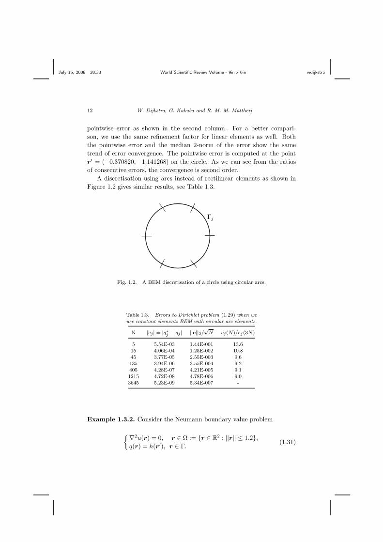
A discretisation using arcs instead of rectilinear elements as shown in
Figure 1.2 gives similar results, see Table 1.3.
Γj
Fig. 1.2. A BEM discretisation of a circle using circular arcs.
Table 1.3. Errors to Dirichlet problem (1.29) when weuse constant elements BEM with circular arc elements.
N |ej| = |q∗j − qj | ||e||2/√
N ej(N)/ej (3N)
5 5.54E-03 1.44E-001 13.615 4.06E-04 1.25E-002 10.845 3.77E-05 2.55E-003 9.6135 3.94E-06 3.55E-004 9.2405 4.28E-07 4.21E-005 9.11215 4.72E-08 4.78E-006 9.03645 5.23E-09 5.34E-007 -
Example 1.3.2. Consider the Neumann boundary value problem
∇2u(r) = 0, r ∈ Ω := r ∈ R2 : ||r|| ≤ 1.2,
q(r) = h(r′), r ∈ Γ.(1.31)
July 15, 2008 20:33 World Scientific Review Volume - 9in x 6in wdijkstra
Condition numbers and local errors in the boundary element method 13
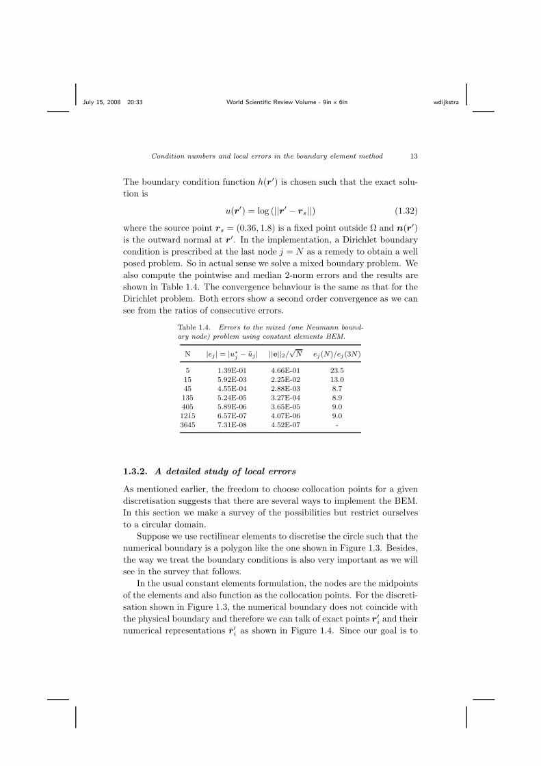
The boundary condition function h(r′) is chosen such that the exact solu-
tion is
u(r′) = log (||r′ − rs||) (1.32)
where the source point rs = (0.36, 1.8) is a fixed point outside Ω and n(r′)
is the outward normal at r′. In the implementation, a Dirichlet boundary
condition is prescribed at the last node j = N as a remedy to obtain a well
posed problem. So in actual sense we solve a mixed boundary problem. We
also compute the pointwise and median 2-norm errors and the results are
shown in Table 1.4. The convergence behaviour is the same as that for the
Dirichlet problem. Both errors show a second order convergence as we can
see from the ratios of consecutive errors.
Table 1.4. Errors to the mixed (one Neumann bound-ary node) problem using constant elements BEM.
N |ej | = |u∗
j − uj | ||e||2/√
N ej(N)/ej(3N)
5 1.39E-01 4.66E-01 23.515 5.92E-03 2.25E-02 13.045 4.55E-04 2.88E-03 8.7135 5.24E-05 3.27E-04 8.9405 5.89E-06 3.65E-05 9.01215 6.57E-07 4.07E-06 9.03645 7.31E-08 4.52E-07 -
1.3.2. A detailed study of local errors
As mentioned earlier, the freedom to choose collocation points for a given
discretisation suggests that there are several ways to implement the BEM.
In this section we make a survey of the possibilities but restrict ourselves
to a circular domain.
Suppose we use rectilinear elements to discretise the circle such that the
numerical boundary is a polygon like the one shown in Figure 1.3. Besides,
the way we treat the boundary conditions is also very important as we will
see in the survey that follows.
In the usual constant elements formulation, the nodes are the midpoints
of the elements and also function as the collocation points. For the discreti-
sation shown in Figure 1.3, the numerical boundary does not coincide with
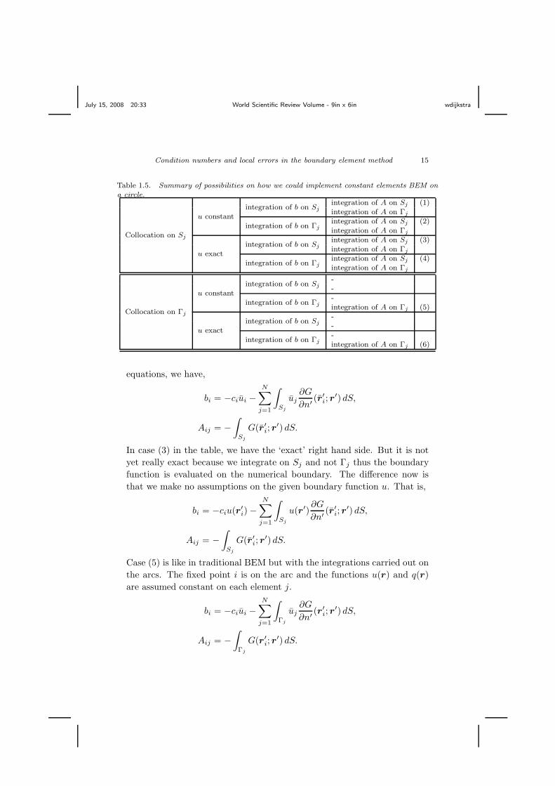
the physical boundary and therefore we can talk of exact points r′i and their
numerical representations r′i as shown in Figure 1.4. Since our goal is to
July 15, 2008 20:33 World Scientific Review Volume - 9in x 6in wdijkstra
14 W. Dijkstra, G. Kakuba and R. M. M. Mattheij
Γj
Sj
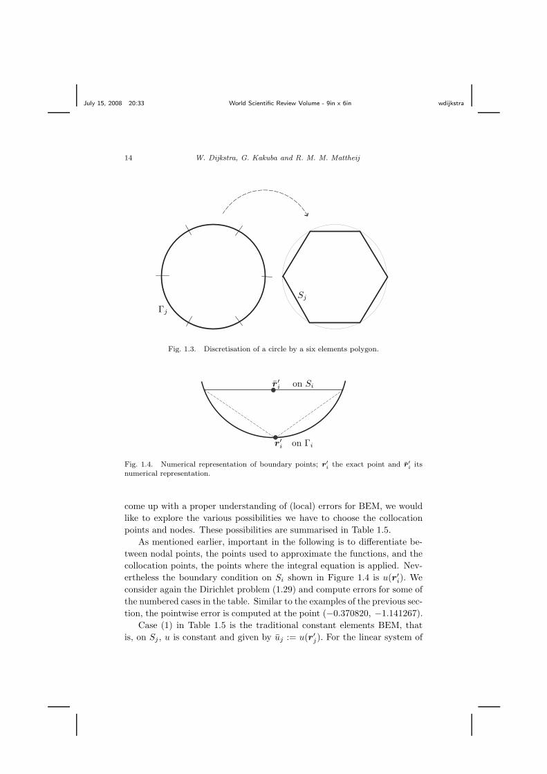
Fig. 1.3. Discretisation of a circle by a six elements polygon.
r′i on Si
r′i on Γi
Fig. 1.4. Numerical representation of boundary points; r′
i the exact point and r′
i itsnumerical representation.
come up with a proper understanding of (local) errors for BEM, we would
like to explore the various possibilities we have to choose the collocation
points and nodes. These possibilities are summarised in Table 1.5.
As mentioned earlier, important in the following is to differentiate be-
tween nodal points, the points used to approximate the functions, and the
collocation points, the points where the integral equation is applied. Nev-
ertheless the boundary condition on Si shown in Figure 1.4 is u(r′i). We
consider again the Dirichlet problem (1.29) and compute errors for some of
the numbered cases in the table. Similar to the examples of the previous sec-
tion, the pointwise error is computed at the point (−0.370820, −1.141267).
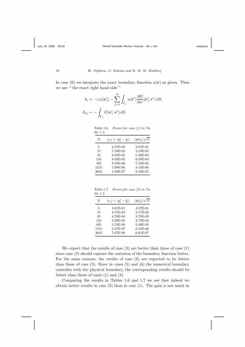
Case (1) in Table 1.5 is the traditional constant elements BEM, that
is, on Sj , u is constant and given by uj := u(r′j). For the linear system of
July 15, 2008 20:33 World Scientific Review Volume - 9in x 6in wdijkstra
Condition numbers and local errors in the boundary element method 15
Table 1.5. Summary of possibilities on how we could implement constant elements BEM ona circle.
Collocation on Sj
u constantintegration of b on Sj
integration of A on Sj (1)integration of A on Γj
integration of b on Γjintegration of A on Sj (2)integration of A on Γj
u exactintegration of b on Sj
integration of A on Sj (3)integration of A on Γj
integration of b on Γjintegration of A on Sj (4)integration of A on Γj
Collocation on Γj
u constantintegration of b on Sj
--
integration of b on Γj-integration of A on Γj (5)
u exactintegration of b on Sj
--
integration of b on Γj-integration of A on Γj (6)
equations, we have,
bi = −ciui −N
∑
j=1
∫
Sj
uj∂G
∂n′(r′i; r
′) dS,
Aij = −
∫
Sj
G(r′i; r′) dS.
In case (3) in the table, we have the ‘exact’ right hand side. But it is not
yet really exact because we integrate on Sj and not Γj thus the boundary
function is evaluated on the numerical boundary. The difference now is
that we make no assumptions on the given boundary function u. That is,
bi = −ciu(r′i) −
N∑
j=1
∫
Sj
u(r′)∂G
∂n′(r′i; r
′) dS,
Aij = −
∫
Sj
G(r′i; r′) dS.
Case (5) is like in traditional BEM but with the integrations carried out on
the arcs. The fixed point i is on the arc and the functions u(r) and q(r)
are assumed constant on each element j.
bi = −ciui −N
∑
j=1
∫
Γj
uj∂G
∂n′(r′i; r
′) dS,
Aij = −
∫
Γj
G(r′i; r′) dS.
July 15, 2008 20:33 World Scientific Review Volume - 9in x 6in wdijkstra
16 W. Dijkstra, G. Kakuba and R. M. M. Mattheij
In case (6) we integrate the exact boundary function u(r) as given. Thus
we use “ the exact right hand side ”
bi = −ciu(r′i) −
N∑
j=1
∫
Γj
u(r′)∂G
∂n′(r′i; r
′) dS,
Aij = −
∫
Γj
G(r′i; r′) dS.
Table 1.6. Errors for case (1) in Ta-ble 1.5.
N |ej | = |qej − qj | ||e||2/
√N
5 6.57E-02 2.81E-0115 7.58E-03 3.53E-0245 8.04E-04 5.40E-03135 8.82E-05 6.58E-04405 9.76E-06 7.53E-051215 1.08E-06 8.45E-063645 1.20E-07 9.42E-07
Table 1.7. Errors for case (3) in Ta-ble 1.5.
N |ej | = |qej − qj | ||e||2/
√N
5 3.01E-01 4.57E-0115 4.57E-03 2.17E-0245 4.76E-04 3.70E-03135 5.20E-05 4.73E-04405 5.74E-06 5.49E-051215 6.37E-07 6.19E-063645 7.07E-08 6.91E-07
We expect that the results of case (3) are better than those of case (1)
since case (3) should capture the variation of the boundary function better.
For the same reasons, the results of case (6) are expected to be better
than those of case (5). Since in cases (5) and (6) the numerical boundary
coincides with the physical boundary, the corresponding results should be
better than those of cases (1) and (3).
Comparing the results in Tables 1.6 and 1.7 we see that indeed we
obtain better results in case (3) than in case (1). The gain is not much in
July 15, 2008 20:33 World Scientific Review Volume - 9in x 6in wdijkstra
Condition numbers and local errors in the boundary element method 17
Table 1.8. Errors for case (5) in Ta-ble 1.5.
N |ej | = |qej − qj | ||e||2/
√N
5 5.54E-03 1.44E-0115 4.06E-04 1.25E-0245 3.77E-05 2.55E-03135 3.94E-06 3.55E-04405 4.28E-07 4.21E-051215 4.72E-08 4.78E-063645 5.23E-09 5.34E-07
Table 1.9. Errors for case (6) in Ta-ble 1.5.
N |ej | = |qej − qj | ||e||2/
√N
5 2.96E-02 1.59E-0115 4.05E-04 1.24E-0245 3.62E-05 2.40E-03135 3.88E-06 3.49E-04405 4.26E-07 4.19E-051215 4.31E-08 4.77E-063645 1.66E-08 5.34E-07
this example and this is because of the smooth variation of the boundary
condition function on the large part of the boundary. This also explains the
little difference between the results in Tables 1.8 and 1.9. As we expected,
the results of cases (5) and (6) are better than those of cases (1) and (3)
respectively. We see that the pointwise errors in Table 1.8 are at least one
order smaller than those in Table 1.6.
1.4. Large condition numbers
In all practical applications of the BEM a linear system needs to be solved
eventually. In most cases it is assumed that the condition number of the
system matrix is moderate, i.e. the linear system has a unique solution and
can be solved accurately. However it is not very clear if this is always true.
It is known that the condition number of the BEM matrix in potential
problems with Dirichlet conditions depends on the size and shape of the
domain on which the potential problem is defined.4–7 On most domains
the condition number is moderate, but on certain domains the condition
July 15, 2008 20:33 World Scientific Review Volume - 9in x 6in wdijkstra
18 W. Dijkstra, G. Kakuba and R. M. M. Mattheij
number becomes infinitely large.
When the BEM is applied to the Laplace equation with Dirichlet con-
ditions on a circular domain, the condition number of the BEM matrix can
be computed analytically.13,14 Here, rectilinear elements are used and a
constant approximation of the functions at each element. It can be shown
that the condition number depends on the radius R of the circle and the
number of boundary elements N according to
cond(G) =max
(
12 , | logR|
)
min(
1N , | logR|
) . (1.33)
This leads to the observation that the condition number is infinitely large
when the radius of the circle is equal to one. Hence the size of the domain
affects the condition number of the BEM matrix, and consequently it also
affects the solvability of the linear system. This introduces a remarkable
phenomenon; the solvability of a linear system in the BEM depends on the
size of the domain.
For the potential problem with Neumann conditions the correspond-
ing BEM matrix is always infinitely large, since this problem is ill-posed,
regardless of the size and shape of the domain. The question then arises
whether we may expect infinitely large condition numbers when solving po-
tential problems with mixed boundary conditions. In this case, the BEM
matrix is a composite matrix, consisting of a number of columns from the
Dirichlet BEM matrix, and a number of columns from the Neumann BEM
matrix. The first matrix is ill-conditioned on some domains, the latter is
ill-conditioned always. It is not a-priori clear how this affects the condition
number of the composite matrix.
For the Laplace equation with mixed conditions on a circular domain
it is possible to give an estimate for the BEM matrix.15 Again it shows
that for the unit circle the condition number is infinitely large. Hence, the
mixed problem seems to inherit the solvability problem from the Dirichlet
problem.
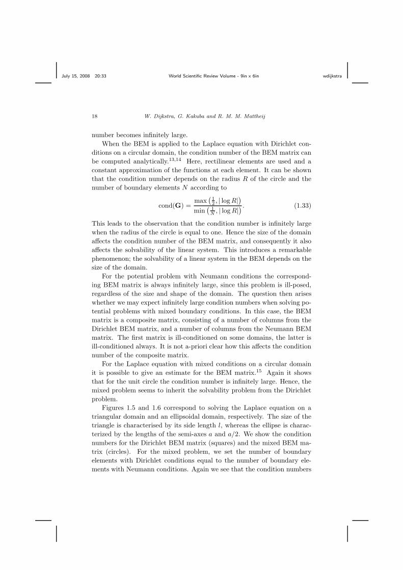
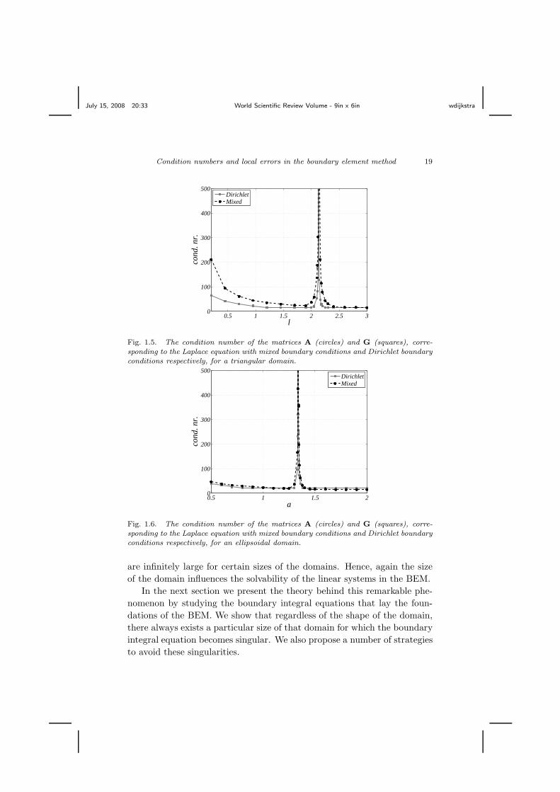
Figures 1.5 and 1.6 correspond to solving the Laplace equation on a
triangular domain and an ellipsoidal domain, respectively. The size of the
triangle is characterised by its side length l, whereas the ellipse is charac-
terized by the lengths of the semi-axes a and a/2. We show the condition
numbers for the Dirichlet BEM matrix (squares) and the mixed BEM ma-
trix (circles). For the mixed problem, we set the number of boundary
elements with Dirichlet conditions equal to the number of boundary ele-
ments with Neumann conditions. Again we see that the condition numbers
July 15, 2008 20:33 World Scientific Review Volume - 9in x 6in wdijkstra
Condition numbers and local errors in the boundary element method 19
0.5 1 1.5 2 2.5 30
100
200
300
400
500
l
con
d.
nr.
DirichletMixed
Fig. 1.5. The condition number of the matrices A (circles) and G (squares), corre-sponding to the Laplace equation with mixed boundary conditions and Dirichlet boundaryconditions respectively, for a triangular domain.
0.5 1 1.5 20
100
200
300
400
500
a
con
d.
nr.
DirichletMixed
Fig. 1.6. The condition number of the matrices A (circles) and G (squares), corre-sponding to the Laplace equation with mixed boundary conditions and Dirichlet boundaryconditions respectively, for an ellipsoidal domain.
are infinitely large for certain sizes of the domains. Hence, again the size
of the domain influences the solvability of the linear systems in the BEM.
In the next section we present the theory behind this remarkable phe-
nomenon by studying the boundary integral equations that lay the foun-
dations of the BEM. We show that regardless of the shape of the domain,
there always exists a particular size of that domain for which the boundary
integral equation becomes singular. We also propose a number of strategies
to avoid these singularities.
July 15, 2008 20:33 World Scientific Review Volume - 9in x 6in wdijkstra
20 W. Dijkstra, G. Kakuba and R. M. M. Mattheij
1.5. Condition numbers in potential problems
This section investigates the condition numbers of the system matrices that
appear in the BEM when applied to potential problems. We analyse po-
tential problems with Dirichlet and mixed boundary conditions and show
that these problems do not always have a unique solution. This happens
when the domains on which the potential problems are defined have loga-
rithmic capacity equal to one. We will proceed by introducing the concept
of logarithmic capacity.
1.5.1. Logarithmic capacity
To study the uniqueness properties of the Dirichlet and the mixed problem
we need to introduce the notion of logarithmic capacity. We define the
energy integral I by a double integral over a contour Γ,
I(q) :=
∫
Γ
∫
Γ
log1
‖r − r′‖q(r)q(r′)dΓrdΓr′ (1.34)
and the logarithmic capacity Cl(Γ) is related to this integral by
− logCl(Γ) := infqI(q). (1.35)
Here the infimum is taken over all functions q with the restriction that∫
Γ
q(r)dΓr = 1. (1.36)
Let us give a physical interpretation of the logarithmic capacity. For
simplicity let the domain Ω be contained in the disc with radius 1/2. In
that case it can be shown that the integral I(q) is positive. The function q
can be seen as a charge distribution over a conducting domain Ω. Faraday
demonstrated that this charge will only reside at the exterior boundary of
the domain, in our case at Γ. We normalize q in such a way that the total
amount of charge at Γ is equal to one, cf. condition (1.36). The function
1
2π
∫
Γ
log1
‖r − r′‖q(r′)dΓr′ ≡ (Ksq)(r) (1.37)
is identified as the potential due to the charge distribution q. Note that the
integral I can also be written as
I(q) = 2π
∫
Γ
(Ksq)(r)q(r)dΓr . (1.38)
Hence I can be seen as the energy of the charge distribution q. The charge
will distribute itself over Γ in such a way that the energy I is minimized.
July 15, 2008 20:33 World Scientific Review Volume - 9in x 6in wdijkstra
Condition numbers and local errors in the boundary element method 21
So the quantity − logCl(Γ) is the minimal amount of energy. Hence the
logarithmic capacity Cl(Γ) is a measure for the capability of the boundary
Γ to support a unit amount of charge.
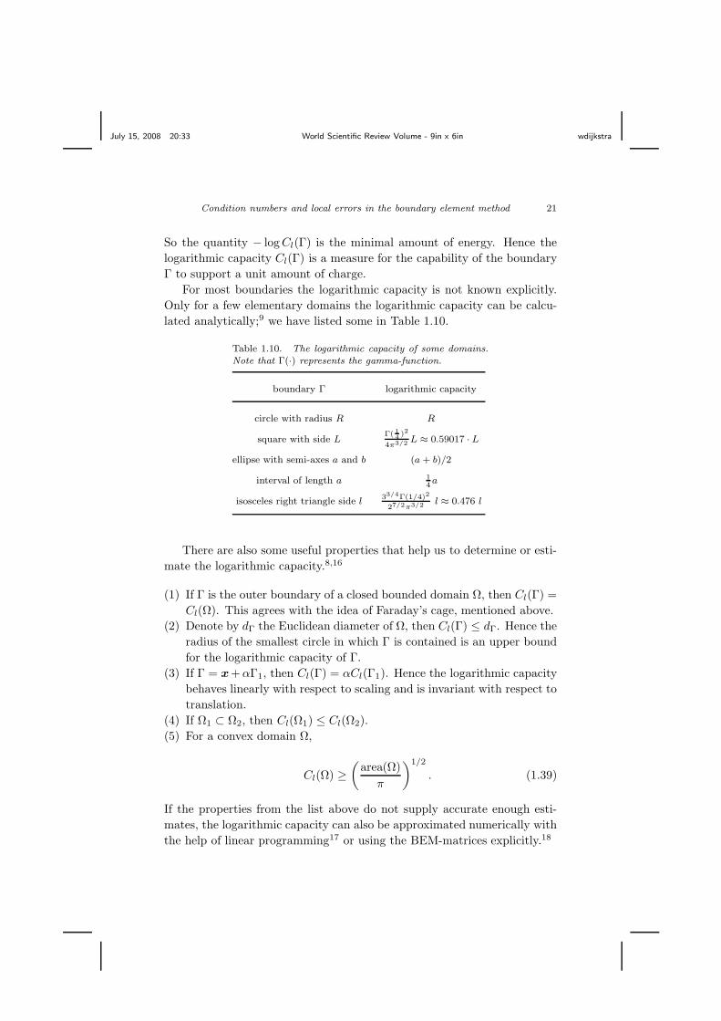
For most boundaries the logarithmic capacity is not known explicitly.
Only for a few elementary domains the logarithmic capacity can be calcu-
lated analytically;9 we have listed some in Table 1.10.
Table 1.10. The logarithmic capacity of some domains.Note that Γ(·) represents the gamma-function.
boundary Γ logarithmic capacity
circle with radius R R
square with side LΓ( 1
4)2
4π3/2L ≈ 0.59017 · L
ellipse with semi-axes a and b (a + b)/2
interval of length a 14a
isosceles right triangle side l33/4Γ(1/4)2
27/2π3/2l ≈ 0.476 l
There are also some useful properties that help us to determine or esti-
mate the logarithmic capacity.8,16
(1) If Γ is the outer boundary of a closed bounded domain Ω, then Cl(Γ) =
Cl(Ω). This agrees with the idea of Faraday’s cage, mentioned above.
(2) Denote by dΓ the Euclidean diameter of Ω, then Cl(Γ) ≤ dΓ. Hence the
radius of the smallest circle in which Γ is contained is an upper bound
for the logarithmic capacity of Γ.
(3) If Γ = x+αΓ1, then Cl(Γ) = αCl(Γ1). Hence the logarithmic capacity
behaves linearly with respect to scaling and is invariant with respect to
translation.
(4) If Ω1 ⊂ Ω2, then Cl(Ω1) ≤ Cl(Ω2).
(5) For a convex domain Ω,
Cl(Ω) ≥
(
area(Ω)
π
)1/2
. (1.39)
If the properties from the list above do not supply accurate enough esti-
mates, the logarithmic capacity can also be approximated numerically with
the help of linear programming17 or using the BEM-matrices explicitly.18
July 15, 2008 20:33 World Scientific Review Volume - 9in x 6in wdijkstra
22 W. Dijkstra, G. Kakuba and R. M. M. Mattheij
1.5.2. Dirichlet problem
We consider the Laplace equation (1.1) with Dirichlet boundary conditions,
with corresponding BIE (1.2). For the single layer operator Ks in this BIE
we have the following result.
Theorem 1.3. There exists a nonzero qe such that
(Ksqe)(r) = −1
2πlogCl(Γ), r ∈ Γ. (1.40)
Sketch of proof. In the following we briefly present the major steps in
the proof of the theorem.8,19,20 We observe that the energy integral (1.34)
takes values −∞ < I(q) ≤ ∞. If the infimum of the energy integral is
infinitely large, then by definition the logarithmic capacity is equal to zero.
Suppose that Cl(Γ) > 0 and thus −∞ < I(q) <∞. It is proven [8, p. 282]
that for each boundary Γ there exists a unique minimizer qe of I(q), i.e.
I(qe) = infqI(q) = − logCl(Γ) with
∫
Γ
qe(r)dΓr = 1. (1.41)
For the minimizer qe the following result is proven [8, p. 287]. Let Γ be the
boundary of a closed bounded domain with positive logarithmic capacity
and a connected complement. Then 2πKsqe ≤ − logCl(Γ) in the whole
plane and 2πKsqe = − logCl(Γ) at Γ, except possibly for a subset which
has zero logarithmic capacity.
Theorem 1.3 leads to the following result.
Corollary 1.1. If Cl(Γ) = 1 there exists a nonzero qe such that Ksqe = 0.
Thus in the specific case that Cl(Γ) = 1 the single layer operator Ks admits
an eigenfunction qe with zero eigenvalue. Hence Ks is not positive definite
and the Dirichlet problem does not have a unique solution.
If the boundary integral equation does not have a unique solution, we
may expect that also its discrete counterpart, the linear system, does not
have a unique solution. That is, the linear system is singular, or at least
ill-conditioned. This is reflected by the condition number of the system
matrix, as show in Figures 1.5 and 1.6. Here the condition number of
the BEM matrix is plotted for two problems: the Laplace equation with
Dirichlet conditions on a triangular and an ellipsoidal domain. The triangle
is an isosceles right triangle with sides of length l. For such a triangle the
July 15, 2008 20:33 World Scientific Review Volume - 9in x 6in wdijkstra
Condition numbers and local errors in the boundary element method 23
logarithmic capacity is given by
Cl(triangle) =33/4Γ2(1/4)
27/2π3/2l ≈ 0.476 l. (1.42)
This implies that the condition number will be large when the scaling pa-
rameter l is close to the critical scaling l∗ := 1/0.476 ≈ 2.1. The ellipse
has semi-axes of length a and a/2, which has logarithmic capacity equal to
3a/4. Hence we may expect a large condition number when the scaling pa-
rameter a is close to a∗ := 4/3. We observe that the condition number for
the Dirichlet case (solid line) is indeed infinitely large for these two critical
scalings.
If we rescale the domain such that the Euclidean diameter is smaller
than one, then the second property in Section 1.5.1 shows us that the
logarithmic capacity will also be smaller than one. In this way we can
guarantee a unique solution of the BIE and thus a low condition number.
Recall that the non-trivial solution qe of the homogeneous BIE Ksq = 0
has a contour integral equal to 1. At the same time we realize that a
solution q of Ksq = 0 has to satisfy∫
Γ
qdΓ =
∫
Ω
∆udΩ = 0, (1.43)
where we make use of Gauss’ theorem. By supplementing this requirement
for q to the BIE, we exclude the possibility that qe is a solution of the ho-
mogeneous BIE. This provides a second strategy to ensure unique solutions
of the BIE.
A third option to guarantee a unique solution is to adjust the integral
operator Ks. Note that the function Gα,
Gα(r; r′) :=1
2πlog
α
‖r − r′‖, α ∈ R
+, (1.44)
is also a fundamental solution for the Laplace operator. The corresponding
single layer potential reads
Ksαq :=
1
2π
∫
Γ
logα
‖r − r′‖q(r′)dΓr′ = Ksq +
logα
2π
∫
Γ
qdΓ. (1.45)
For the minimizer qe we get
Ksαqe = Ksqe +
logα
2π
∫
Γ
qedΓ = −1
2πlogCl(Γ) +
1
2πlogα
=1
2πlog
α
Cl(Γ). (1.46)
July 15, 2008 20:33 World Scientific Review Volume - 9in x 6in wdijkstra
24 W. Dijkstra, G. Kakuba and R. M. M. Mattheij
This is only equal to zero if α = Cl(Γ). We may choose α any positive real
number unequal to Cl(Γ) and obtain Ksαqe 6= 0. In that case qe is no longer
an eigenfunction of the single layer potential operator with zero eigenvalue.
Hence the BIE (1.2) with Dirichlet conditions is uniquely solvable if Ks is
replaced by Ksα.19,21 The advantage of this procedure is that we do not
need a rescaling of the domain, nor do we have to add an extra equation.
Furthermore, we do not need to know the logarithmic capacity explicitly;
a rough estimate of the capacity sufficies to choose α such that α 6= Cl(Γ).
There are also ways to ensure a unique solution of the BIE for the
Laplace equation that can be used without having to know the logarithmic
capacity. For instance, adding an extra collocation node at the interior or
exterior of the domain can change the BIE in such a way that it is not singu-
lar any longer.22 This does depend on the location of the extra collocation
node though. Another option is to use the hypersingular formulation of the
BIE.23 The hypersingular BIE is the normal derivative of the standard BIE
and does not involve the single layer operator. As a consequence the BIE
does not become singular at certain domains.
1.5.3. Mixed problem
We consider the Laplace equation with mixed boundary conditions,
∇2u = 0, r ∈ Ω,
u = u, r ∈ Γ1,
q = q, r ∈ Γ2, (1.47)
where Γ = Γ1 ∪ Γ2. To investigate this boundary value problem we have to
rewrite the BIE in (1.2). For i = 1, 2 we introduce the functions ui := u|Γi
and qi := q|Γi and the boundary integral operators
(Ksi q)(r) :=
∫
Γi
G(r; r′)q(r′)dΓr′ , r ∈ Γ, (1.48a)
(Kdi u)(r) :=
∫
Γi
∂
∂nyG(r; r′)u(r′)dΓr′ , r ∈ Γ. (1.48b)
Note that the boundary conditions in (1.47) provide u1 = u and q2 = q. By
distinguishing r ∈ Γ1 and r ∈ Γ2, we write (1.2) as a system of two BIEs,
Kd2u2 −Ks
1q1 = Ks2q −
1
2u−Kd
1u, r ∈ Γ1, (1.49a)
1
2u2 + Kd
2u2 −Ks1q1 = Ks
2q −Kd1u, r ∈ Γ2. (1.49b)
July 15, 2008 20:33 World Scientific Review Volume - 9in x 6in wdijkstra
Condition numbers and local errors in the boundary element method 25
In this system all prescribed boundary data are at the right-hand side of
the equations.
Theorem 1.4. If Cl(Γ) = 1, the homogeneous equations of (1.49a) and
(1.49b) have a non-trivial solution pair (q1, u2).
Sketch of proof. We have to find a non-trivial pair of functions (q1, u2)
such that the left-hand sides of (1.49a) and (1.49b) are equal to zero when
Cl(Γ) = 1. It can be shown that such a pair of functions exists by using
information from the Dirichlet problem.11
Theorem 1.4 tells us that the BIE for the mixed problem does not have
a unique solution when Cl(Γ) = 1, i.e. the BIE is singular. Moreover the
division of Γ into a part Γ1 with Dirichlet conditions and a part Γ2 with
Neumann conditions does not play a role in this. It does not make a
difference whether we take Γ1 very small or very large; the singular BIE
relates solely to the whole boundary Γ.
In Figures 1.5 and 1.6 we observe that indeed the condition number for
the mixed problems is infinitely large at (almost) the same scalings as for
the Dirichlet problems, agreeing with the theory. The small difference that
is present is caused by numerical inaccuracies due to the discretisation.
To guarantee a unique solution for the mixed problem we have the same
options as for the Dirichlet problem. The simplest remedy is to rescale the
domain, thus avoiding a unit logarithmic capacity. A second option is to
demand that the function q has a zero contour integral. Since part of q is
already prescribed this yields the following condition for the unknown part
of q,
∫
Γ1
q1dΓ = −
∫
Γ2
qdΓ. (1.50)
As a last option to obtain nonsingular BIEs, we can also replace the single
layer operator Ks by Ksα, see Section 1.5.2.
1.6. Condition numbers in flow problems
The Laplace equation and the Stokes equations have at least one thing in
common: the Laplace operator appears in both equations. As we have seen
in the previous section, the Laplace equation may lead to a singular BIE
for certain critical domains. The question arises whether this is also the
July 15, 2008 20:33 World Scientific Review Volume - 9in x 6in wdijkstra
26 W. Dijkstra, G. Kakuba and R. M. M. Mattheij
case for the equations in viscous flow problems: can the corresponding BIEs
become singular on certain critical domains?
In this section we study the BIEs following from the Stokes equations.
In particular we focus on the eigenvalues of the integral operators. It is
shown that for certain critical domains these integral operators admit zero
eigenvalues. Hence, again we find that the BIEs become singular for a
number of critical domains.
For the Laplace equation it is possible to a-priori determine the critical
domains. For a number of simple domains, the logarithmic capacity can
be used to exactly compute the critical size. For more involved domains
the logarithmic capacity can be used to estimate the critical size of the
domain. Unfortunately the critical domains for the Stokes equations do
not coincide with the critical domains for the Laplace equations. Hence
we cannot use the logarithmic capacity to a-priori determine the critical
domains on which the BIEs for Stokes equations become singular. It is only
by numerical experiments that we can distinguish the critical domains.
Let Ω be a two-dimensional simply-connected domain with a piece-wise
smooth boundary Γ. The Stokes equations for a viscous flow in Ω read
∇2v −∇p = 0,
∇.v = 0, (1.51)
where v is the velocity field of the fluid and p its pressure. Let Γ be divided
into a part Γ1 on which the velocity v is prescribed, and a part Γ2 on which
the pressure p is prescribed, Γ = Γ1
⋃
Γ2. Hence the Stokes equations are
subject to the boundary conditions
v = v, r ∈ Γ1,
p = p, r ∈ Γ2. (1.52)
Either Γ1 or Γ2 can be empty, leading to a purely Neumann or Dirichlet
problem respectively. The Stokes equations in differential form can be
transformed to a set of two BIEs6,24,25
1
2vi(r) +
∫
Γ
qij(r, r′)vj(r
′)dΓr′
=
∫
Γ
uij(r, r′)bj(r
′)dΓr′ , r ∈ Γ, i = 1, 2. (1.53)
Here a repeated index means summation over all possible values of that
index. The vector function b is the normal stress at the fluid boundary,
b := σ(p,v)n, (1.54)
July 15, 2008 20:33 World Scientific Review Volume - 9in x 6in wdijkstra
Condition numbers and local errors in the boundary element method 27
with n the outward unit normal at the boundary and the stress tensor σ
defined by
σij(p,v) := −pδij +( ∂vi
∂xj+∂vj
∂xi
)
. (1.55)
Hence the boundary integral formulation involves two variables, the velocity
v and the normal stress b. In correspondence to (1.52), at each point of
the boundary either v or b is prescribed,
v = v, r ∈ Γ1,
b = −pn, r ∈ Γ2.(1.56)
The kernels uij and qij in the integral operators are defined as
qij(r, r′) :=
1
π
(xi − yi)(xj − yj)(xk − yk)nk
‖r − r′‖4,
uij(r, r′) :=
1
4π
δij log1
‖r − r′‖+
(xi − yi)(xj − yj)
‖r − r′‖2
, (1.57)
for i, j = 1, 2. We introduce boundary integral operators,
(Gϕ)i(r) :=
∫
Γ
uij(r, r′)ϕj(r
′)dΓr′ ,
(Hψ)i(r) :=
∫
Γ
qij(r, r′)ψj(r
′)dΓr′ , (1.58)
which enables us to write (1.53) as
(1
2I + H)v = Gb. (1.59)
The operators G and H are called the single and double layer operator
for the Stokes equations. For the Dirichlet problem the velocity v at the
boundary is given (Γ2 = ∅) and we would like to reconstruct the normal
stress b at the boundary. To this end we need to invert the operator G.
This can only be done when all eigenvalues of G are unequal to zero. In this
section we investigate under which conditions G admits a zero eigenvalue.
For the mixed problem the velocity at Γ1 is prescribed and the normal
stress at Γ2 is prescribed. We would like to reconstruct the unknown veloc-
ity at Γ2 and the unknown normal stress at Γ1. After rearranging known
and unknown terms (see Section 1.6.2) we again need to invert a boundary
integral operator. This can only be done when all eigenvalues of the oper-
ator are unequal to zero. We will show that zero eigenvalues occur under
the same conditions as for the Dirichlet problem.
July 15, 2008 20:33 World Scientific Review Volume - 9in x 6in wdijkstra
28 W. Dijkstra, G. Kakuba and R. M. M. Mattheij
1.6.1. Flow problems with Dirichlet boundary conditions
In this subsection we study the solvability of the BIE (1.59) with Dirich-
let conditions on a piece-wise smooth closed boundary Γ. We search for
eigenfunctions b of the boundary integral operator G with zero eigenvalue,
hence Gb = 0. If such eigenfunctions exist, the boundary integral operator
G is not invertible and the integral equation (1.59) is not uniquely solvable.
First we show that at least one such eigenfunction with zero eigenvalue
exists.
Theorem 1.5. For any smooth boundary Γ the outward unit normal n(r)
is an eigenfunction of the boundary integral operator G with eigenvalue zero.
Proof. The i-th component of Gn equals
(Gn)i =
∫
Γ
uij(r, r′)nj(r
′)dΓr′
=1
4π
∫
Γ
[
δij log1
‖r − r′‖+
(xi − yi)(xj − yj)
‖r − r′‖2
]
nj(r′)dΓr′
=1
4π
∫
Ω
∂
∂xj
[
δij log1
‖r − r′‖+
(xi − yi)(xj − yj)
‖r − r′‖2
]
dΩy
= −
∫
Ω
∂
∂xjui
jdΩy = −
∫
Ω
∇.uidΩ = 0. (1.60)
Here the vector ui is the velocity due to a Stokeslet ,24 i.e. the velocity field
induced by a point force in the ei-direction. This velocity field satisfies the
incompressibility condition ∇.ui = 0.
In the sequel of this section we assume that the solutions of the Dirichlet
problem (1.59) are sought in a function space that excludes the normal.
Hence the eigenfunctions b of G we are looking for are perpendicular to n.
We now show that for each boundary Γ there exist (at most) two critical
scalings of the boundary such that the operator G in the Dirichlet problem
(1.59) is not invertible. This phenomenon has been observed and proven26
and we will partly present the analysis here. The scaling for which the
operator G is not invertible is called a critical scaling, and the corresponding
boundary a critical boundary. The domain that is enclosed by the critical
boundary is referred to as the critical domain.
July 15, 2008 20:33 World Scientific Review Volume - 9in x 6in wdijkstra
Condition numbers and local errors in the boundary element method 29
Theorem 1.6. For all given functions f and constant vectors d the system
of equations
Gb+ c = f ,∫
ΓbdΓ = d,
(1.61)
has a unique solution pair (b, c), where b is a function and c a constant
vector.
Sketch of proof. The main idea is to show that the operator that maps
the pair (b, c) to the left-hand side of (1.61) is an isomorphism.26
We proceed by introducing the two unit vectors e1 = [1, 0]T and e2 =
[0, 1]T . Theorem 1.6 guarantees that two pairs (b1, c1) and (b2, c2) exist
that are the unique solutions to the two systems
Gb1 + c1 = 0,∫
Γ b1dΓ = e1,
Gb2 + c2 = 0,∫
Γ b2dΓ = e2.
(1.62)
We define the matrix CΓ as CΓ := [c1|c2].
Theorem 1.7. If det(CΓ) = 0, then the operator G is not invertible.
Proof. Suppose that det(CΓ) = 0, then the columns c1 and c2 are de-
pendent, say c1 = αc2 for some α ∈ R, α 6= 0. In that case
0 =(
Gb1 + c1)
− α(
Gb2 + c2)
= G(b1 − αb2) + αc2 − αc2
= G(b1 − αb2). (1.63)
The function b1 − αb2 cannot be equal to zero, since this requires∫
Γ(b1 − αb2)dΓ to be equal to zero, while we have
∫
Γ
(b1 − αb2)dΓ = e1 − αe2 6= 0. (1.64)
So b1−αb2 is an eigenfunction of G with zero eigenvalue. This eigenfunction
cannot be equal to the normal n, since n also requires∫
Γ ndΓ = 0.
Corollary 1.2. There are (at most) two critical scalings of the domain Γ
for which the operator G is not invertible.
Proof. We rescale the domain Γ by a factor a, i.e. Γ → aΓ. With the
definition of the operator G it can be shown that
Gb→ Gab := −1
4π
∫
Γ
a log a bdΓ + aGb. (1.65)
July 15, 2008 20:33 World Scientific Review Volume - 9in x 6in wdijkstra
30 W. Dijkstra, G. Kakuba and R. M. M. Mattheij
Then the two systems in (1.62) change into
aGbj + cj − 14π
∫
Γ a log a bjdΓ = 0,
a∫
Γ bjdΓ = ej , j = 1, 2.
(1.66)
Define bja := abj for j = 1, 2, then we obtain
Gbja + cj − 1
4π
∫
Γ log a bjadΓ = 0,
∫
Γ bjadΓ = ej , j = 1, 2.
(1.67)
Substituting the second equation into the first equation, we get
Gbja + cj − 1
4π log a ej = 0,∫
Γbj
adΓ = ej , j = 1, 2.(1.68)
These systems have the same form as the original systems in (1.62), except
for the change cj → cj − 14π log a ej for j = 1, 2. Define the new matrix
CaΓ by
CaΓ := CΓ −1
4πlog a I2, (1.69)
then Ga is not invertible when det(CaΓ) = 0. Hence, when 14π log a is an
eigenvalue of CΓ, the operator Ga is not invertible. This implies that, when
CΓ has two distinct eigenvalues, there are two critical scalings a for which
Ga is not invertible. If CΓ has one eigenvalue with double multiplicity these
critical scalings coincide.
The result of Corollary 1.2 shows that the BIEs for the Dirichlet Stokes
equations become singular for certain sizes of the domain. As a conse-
quence, the equations are not uniquely solvable. This solvability problem
is an artifact of the boundary integral formulation; the Stokes equations
in differential form always have a unique solution. In the previous section
a similar phenomenon is observed for the Laplace equation with Dirich-
let conditions; in its differential form the problem is well-posed, while the
corresponding BIE is not solvable at critical boundaries.
For the Laplace equation the critical scaling is related to the logarithmic
capacity of the domain. By calculating or estimating the logarithmic capac-
ity one can determine or estimate the critical domains, without computing
BEM matrices and evaluating their condition numbers. It is this a-priori
information that allows us to modify the standard BEM formulation such
that the BIE become uniquely solvable.
For the Stokes equations, there does not exist an equivalent to the loga-
rithmic capacity. Hence we cannot a-priori determine the critical domains.
July 15, 2008 20:33 World Scientific Review Volume - 9in x 6in wdijkstra
Condition numbers and local errors in the boundary element method 31
One way to determine the critical domains is by computing the BEM-
matrices and evaluating their condition numbers. If the condition number
jumps to infinity for a certain domain, then this domain is a critical domain.
Hence, this strategy requires the solution of many BEM problems.
Another possibility to determine the critical domains is by solving the
systems in (1.62). This yields the matrix CΓ, and subsequently the matrix
CaΓ. By calculating the eigenvalues of the latter matrix the critical scalings
can be found. Again we have to solve two non-standard BEM problems to
compute the critical scalings.
Remark: The BIEs for the Stokes flow in 2D are similar to the equa-
tions for plane elasticity. Hence the BIEs for the latter equations suffer
from the same solvability problems as the Stokes equations. A proof of this
phenomenon for plane elasticity is found in literature27 and is similar to
the proof sketched above.
1.6.2. Flow problems with mixed boundary conditions
In the previous subsection we showed that the boundary integral operator
G for the Dirichlet Stokes equations is not invertible for all domains. In this
subsection we show that this phenomenon extends to the Stokes equations
with mixed boundary conditions.
The starting point is again the BIE for the Stokes equations,
1
2v + Hv = Gb, at Γ. (1.70)
Suppose that the boundary Γ is split into two parts, Γ = Γ1
⋃
Γ2. On Γ1
we prescribe the velocity v1 while the normal stress b1 is unknown. On Γ2
we prescribe the normal stress b2 while the velocity v2 is unknown. The
boundary integral operators G and H are split accordingly,
[Gb]i =
∫
Γ
uijbjdΓ =
∫
Γ1
uijb1jdΓ +
∫
Γ2
uijb2jdΓ =: [G1b1]i + [G2b2]i,
[Hv]i =
∫
Γ
qijvjdΓ =
∫
Γ1
qijv1jdΓ +
∫
Γ2
qijv2jdΓ =: [H1v1]i + [H2v2]i.
(1.71)
With these notations the BIE is written in the following way,
1
2vk + H1v1 + H2v2 = G1b1 + G2b2, at Γk, k = 1, 2. (1.72)
July 15, 2008 20:33 World Scientific Review Volume - 9in x 6in wdijkstra
32 W. Dijkstra, G. Kakuba and R. M. M. Mattheij
We arrange the terms in such a way that all unknowns are at the left-hand
side and all knowns are at the right-hand side,
H2v2 − G1b1 = G2b2 −H1v1 −1
2v1, at Γ1,
1
2v2 + H2v2 − G1b1 = G2b2 −H1v1, at Γ2. (1.73)
Now we can define an operator A that assigns to the pair (b1,v2) the two
functions at the left-hand side of (1.73),[
b1
v2
]
A→
[
H2v2 − G1b1
12v
2 + H2v2 − G1b1
]
(1.74)
To study the invertibility of this operator we need to study the homogeneous
version of the equations in (1.73),
H2v2 − G1b1 = 0, at Γ1,1
2v2 + H2v2 − G1b1 = 0, at Γ2. (1.75)
Theorem 1.8. There are (at most) two scalings of Γ such that the homoge-
neous equations (1.75) have a non-trivial solution, i.e. A is not invertible.
Sketch of proof. We have to find a non-trivial pair of functions (b1,v2)
such that the left-hand sides of (1.75) are equal to zero when Cl(Γ) = 1.
Similar to the Laplacian case, it can be shown that such a pair of functions
exists by using information from the Dirichlet problem.28
This result shows that also the BIE for the Stokes equations with mixed
boundary conditions may become singular. This happens for the same
critical boundaries as for the Stokes equations with Dirichlet boundary
conditions. Hence the mixed problem inherits the singularities from the
Dirichlet problem. The division of the boundary into a Dirichlet and a
Neumann part does not play a role in this.
Note that the Laplace equation exhibits the same behaviour. The
boundary integral equation for the Laplace equation with mixed bound-
ary conditions also inherits the solvability problems from the BIE for the
Dirichlet case.11
1.6.3. Numerical examples
To solve the BIEs (1.59), the boundary Γ is discretised into a set of N
linear elements. At each element the velocity v and normal stress b are
July 15, 2008 20:33 World Scientific Review Volume - 9in x 6in wdijkstra
Condition numbers and local errors in the boundary element method 33
approximated linearly. In this way the BIEs are transformed into a linear
system of algebraic equations (for details about the discretisation we refer
to any BEM handbook29,30). We introduce vectors v and b of length 2N
containing the coefficients of v and b at the nodal points. Then the system
of equations can be written in short-hand notation as
Gb = (1
2I + H)v. (1.76)
Here G and H are the discrete counterparts of the single and double layer
operator.
If the boundary integral operator G is not invertible then its discrete
counterpart, the matrix G is ill-conditioned. To visualize this we compute
the condition number of G: if the condition number is infinitely large, then
the matrix is not invertible. As a consequence, the linear system (1.76) is
singular and cannot be solved for arbitrary right-hand side vectors. If the
condition number is bounded but very large, then still the problem (1.76)
is difficult to solve accurately.
In the following examples we construct the matrix G for a certain
boundary Γ and compute the condition number of this matrix. Then we
rescale the boundary Γ by a factor a, i.e. Γ → aΓ. Again we compute the
condition number of the matrix G. We do this for several values of the
scaling parameter a. According to the theory in the previous sections there
are two critical scalings for which the integral operator G is not invertible.
For these two scalings also the matrix G is not invertible, or at least very
ill-conditioned. Hence we expect that the condition number of G jumps to
infinity at these two scalings. The scaling for which such large condition
numbers appear is again called a critical scaling and has ideally the same
value as the critical scaling defined for the BIE in the previous section.
However, due to the discretisation of the equations, the critical scaling for
the discrete problem may be slightly different from the critical scaling for
the BIE. In the limit N → ∞ these differences vanish.
As the results for the Dirichlet and mixed problems are similar, we do
not present any examples for the mixed case here.
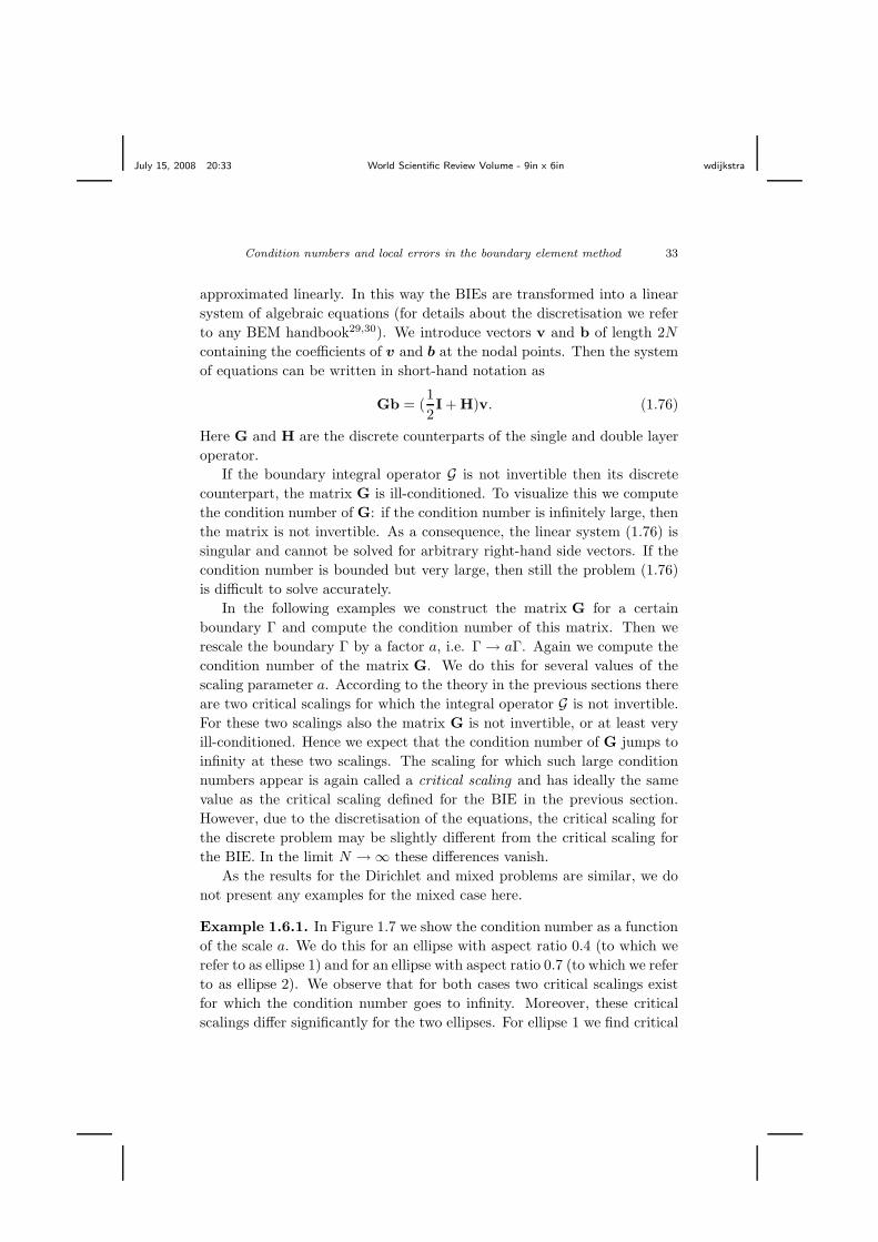
Example 1.6.1. In Figure 1.7 we show the condition number as a function
of the scale a. We do this for an ellipse with aspect ratio 0.4 (to which we
refer to as ellipse 1) and for an ellipse with aspect ratio 0.7 (to which we refer
to as ellipse 2). We observe that for both cases two critical scalings exist
for which the condition number goes to infinity. Moreover, these critical
scalings differ significantly for the two ellipses. For ellipse 1 we find critical
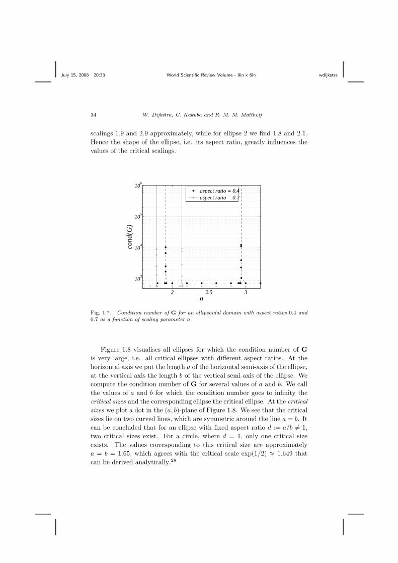
July 15, 2008 20:33 World Scientific Review Volume - 9in x 6in wdijkstra
34 W. Dijkstra, G. Kakuba and R. M. M. Mattheij
scalings 1.9 and 2.9 approximately, while for ellipse 2 we find 1.8 and 2.1.
Hence the shape of the ellipse, i.e. its aspect ratio, greatly influences the
values of the critical scalings.
2 2.5 3
103
104
105
106
a
con
d(G
)
aspect ratio = 0.4aspect ratio = 0.7
Fig. 1.7. Condition number of G for an ellipsoidal domain with aspect ratios 0.4 and0.7 as a function of scaling parameter a.
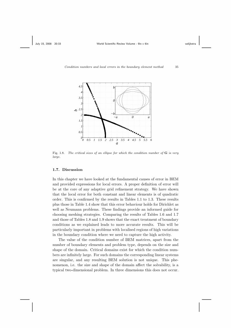
Figure 1.8 visualises all ellipses for which the condition number of G
is very large, i.e. all critical ellipses with different aspect ratios. At the
horizontal axis we put the length a of the horizontal semi-axis of the ellipse,
at the vertical axis the length b of the vertical semi-axis of the ellipse. We
compute the condition number of G for several values of a and b. We call
the values of a and b for which the condition number goes to infinity the
critical sizes and the corresponding ellipse the critical ellipse. At the critical
sizes we plot a dot in the (a, b)-plane of Figure 1.8. We see that the critical
sizes lie on two curved lines, which are symmetric around the line a = b. It
can be concluded that for an ellipse with fixed aspect ratio d := a/b 6= 1,
two critical sizes exist. For a circle, where d = 1, only one critical size
exists. The values corresponding to this critical size are approximately
a = b = 1.65, which agrees with the critical scale exp(1/2) ≈ 1.649 that
can be derived analytically.28
July 15, 2008 20:33 World Scientific Review Volume - 9in x 6in wdijkstra
Condition numbers and local errors in the boundary element method 35
0 0.5 1 1.5 2 2.5 3 3.5 4 4.5 5 5.5 60
0.5
1
1.5
2
2.5
3
3.5
4
4.5
a
b
−a 0 a−b
0
b
Fig. 1.8. The critical sizes of an ellipse for which the condition number of G is verylarge.
1.7. Discussion
In this chapter we have looked at the fundamental causes of error in BEM
and provided expressions for local errors. A proper definition of error will
be at the core of any adaptive grid refinement strategy. We have shown
that the local error for both constant and linear elements is of quadratic
order. This is confirmed by the results in Tables 1.1 to 1.3. These results
plus those in Table 1.4 show that this error behaviour holds for Dirichlet as
well as Neumann problems. These findings provide an informed guide for
choosing meshing strategies. Comparing the results of Tables 1.6 and 1.7
and those of Tables 1.8 and 1.9 shows that the exact treatment of boundary
conditions as we explained leads to more accurate results. This will be
particularly important in problems with localised regions of high variations
in the boundary condition where we need to capture the high activity.
The value of the condition number of BEM matrices, apart from the
number of boundary elements and problem type, depends on the size and
shape of the domain. Critical domains exist for which the condition num-
bers are infinitely large. For such domains the corresponding linear systems
are singular, and any resulting BEM solution is not unique. This phe-
nomenon, i.e. the size and shape of the domain affect the solvability, is a
typical two-dimensional problem. In three dimensions this does not occur.
July 15, 2008 20:33 World Scientific Review Volume - 9in x 6in wdijkstra
36 W. Dijkstra, G. Kakuba and R. M. M. Mattheij
The core of the phenomenon is the logarithmic term in the 2D fundamen-
tal solution for the differential operators, which transforms a scaling of the
domain into an additive term. In three dimensions such a logarithmic term
does not appear in the fundamental solution.
We have presented a number of strategies to avoid critical domains,
which can be implemented easily in existing BEM codes. This will guar-
antee the uniqueness of the BEM solutions for domains of all sizes and
shapes.
For potential problems one can a-priori determine or estimate the criti-
cal domains on which the condition number of the BEM matrix is infinitely
large. This is achieved by exploiting the concept of logarithmic capacity.
Unfortunately, we cannot use this strategy to determine or estimate the
critical domains for flow problems, since an equivalent concept of the loga-
rithmic capacity for flow problems does not yet exist.
In this chapter we have shown that critical domains exist for potential
problems and flow problems, and at the same time critical domains occur
when solving the biharmonic equation with the BEM.31–33 The question
arises whether critical domains exist for a broader class of boundary value
problems. To the authors’ knowledge this is still an open question.
References
1. M. Guiggiani and F. Lombardi, Self-adaptive boundary elements with h-hierachical shape functions., Advances in Engineering Software, Special issueon error estimates and adaptive meshes for FEM/BEM. 15, 269–277, (1992).
2. M. Liang, J. Chen, and S. Yang, Error estimation for boundary elementmethod., Engineering analysis with boundary elements. 23, 257–265, (1999).
3. C. Carsten and E. Stephan, A posteriori error estimates for boundary elementmethods., Mathematics of Computation. 64, 483–500, (1995).
4. G. Hsiao, On the stability of integral equations of the first kind with loga-rithmic kernels, Arch. Ration. Mech. Anal. 94, 179–192, (1986).
5. M. Jaswon and G. Symm, Integral Equation Methods in Potential Theoryand Elastostatics. (Academic Press, London, 1977).
6. H. Power and L. Wrobel, Boundary integral methods in fluid mechanics.(Computational Mechanics Publications, Southampton, 1995).
7. I. Sloan and A. Spence, The Galerkin method for integral equations of thefirst kind with logarithmic kernel: theory, IMA J. Numer. Anal. 8, 105–122,(1988).
8. E. Hille, Analytic Function Theory: vol II. (Ginn, London, 1959).9. N. Landkof, Foundations of Modern Potential Theory. (Springer Verlag,
Berlin, 1972).

July 15, 2008 20:33 World Scientific Review Volume - 9in x 6in wdijkstra
Condition numbers and local errors in the boundary element method 37
10. M. Tsuji, Potential Theory in Modern Function Theory. (Maruzen, Tokyo,1959).
11. W. Dijkstra and R. Mattheij, A relation between the logarithmic capacityand the condition number of the BEM-matrices, Comm. Numer. MethodsEngrg. 23(7), 665–680, (2007).
12. M. Heath, Scientific computing, an introductory survey. (McGraw Hill, NewYork, 2002).
13. S. Christiansen, Condition number of matrices derived from two classes ofintegral equations, Mat. Meth. Appl. Sci. 3, 364–392, (1981).
14. S. Christiansen, On two methods for elimination of non-unique solutions ofan integral equation with logarithmic kernel, Appl. Anal. 13, 1–18, (1982).
15. W. Dijkstra and R. Mattheij, The condition number of the BEM-matrix aris-ing from Laplace’s equation, Electron. J. Bound. Elem. 4(2), 67–81, (2006).
16. R. Barnard, K. Pearce, and A. Solynin, Area, width, and logarithmic capacityof convex sets, Pacific J. Math. 212, 13–23, (2003).
17. J. Rostand, Computing logarithmic capacity with linear programming, Ex-periment. Math. 6, 221–238, (1997).
18. W. Dijkstra and M. Hochstenbach, Numerical approximation of the logarith-mic capacity, Appl. Numer. Math. (2008). submitted.
19. W. McLean, Strongly elliptic systems and boundary integral equations. (Cam-bridge University Press, Cambridge, 2000).
20. Y. Yan and I. Sloan, On integral equations of the first kind with logarithmickernels, J. Integral Equations Appl. 1, 549–579, (1988).
21. C. Constanda, On the solution of the Dirichlet problem for the two-dimensional Laplace equation, Proc. Amer. Math. Soc. 119(3), 877–884,(1993).
22. J. Chen, C. Lee, I. Chen, and J. Lin, An alternative method for degeneratescale problems in boundary element methods for the two-dimensional Laplaceequation, Eng. Anal. Bound. Elem. 26, 559–569, (2002).
23. J. Chen, J. Lin, S. Kuo, and Y. Chiu, Analytical study and numerical ex-periments for degenerate scale problems in boundary element method usingdegenerate kernels and circulants, Eng. Anal. Bound. Elem. 25, 819–828,(2001).
24. O. Ladyzhenskaya, The Mathematical Theory of Viscous IncompressibleFlow. (Gordon and Beach, New York-London, 1963).
25. C. Pozrikidis, Boundary integral and singularity methods for linearized vis-cous flows. (Cambridge University Press, Cambridge, 1992).
26. V. Domınguez and F. Sayas, A BEM-FEM overlapping algorithm for theStokes equation, Appl. Math. Comput. 182, 691–710, (2006).
27. R. Vodicka and V. Mantic, On invertibility of elastic single-layer potentialoperator, J. Elasticity. 74, 147–173, (2004).
28. W. Dijkstra and R. Mattheij, Condition number of the BEM matrix arisingfrom the Stokes equations in 2D, Eng. Anal. Bound. Elem. in press.
29. A. Becker, The Boundary Element Method in Engineering. (McGraw-Hill,Maidenhead, 1992).
30. C. Brebbia, J. Telles, and L. Wrobel, The boundary element method in engi-
July 15, 2008 20:33 World Scientific Review Volume - 9in x 6in wdijkstra
38 W. Dijkstra, G. Kakuba and R. M. M. Mattheij
neering. (McGraw-Hill Book Company, London, 1984).31. B. Fuglede, On a direct method of integral equations for solving the bihar-
monic Dirichlet problem, ZAMM. 61, 449–459, (1981).32. M. Costabel and M. Dauge, On invertibility of the biharmonic single-layer
potential operator, Integr. Equ. Oper. Theory. 24, 46–67, (1996).33. C. Constanda, On the Dirichlet problem for the two-dimensional biharmonic
equation, Mat. Meth. Appl. Sci. 20, 885–890, (1997).
Recommended