Chap 4 Image Enhancement in the Chap 4 Image Enhancement in the Frequency DomainFrequency Domain

Background
• Any periodic function can be expressed as the sum of sines and cosines of different frequencies, each multiplied by a different coefficient.– We called this sum a Fourier series.
• Even function that are not periodic can be expressed as the integral of sines and cosines multiplied by a weighting function.– This formation is the Fourier transform.


Periodic FunctionPeriodic Function
• A function f is periodic with period P greater than zero if– Af(x + P) = Af(x), where A denotes amplitude.
f(x) = sinx, P = 2π, frequency=1/ 2π, A=1.
f(x) = Asinnx, P = 2π/n, frequency=n/ 2 π.
– n↑, frequency↑.

Fourier SeriesFourier Series
• Suppose f(x) is a function defined on the interval [-π,π]. The Fourier series expansion of f(x) is
where an and bn are constants called the Fourier coefficients, and
1
0 )sincos(2
)(n
nn nxbnxaa
xf
nxdxxfb
nxdxxfa
n
n
sin)(1
cos)(1
Coefficients of Any Period T = 2L
• Replace v by πx/L to obtain the Fourier series of the function ƒ(x) of period 2L
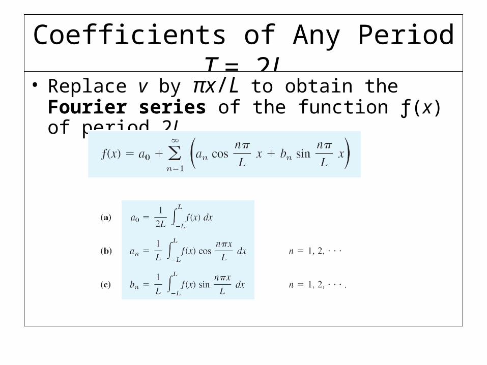
Complex Fourier SeriesComplex Fourier Series• Complex exponentials
– According to Euler’s formula
and so,
Using these two equations we can find the complex exponential form of the trigonometric functions as
jej sincos
sincos)sin()cos( )( jej j
j
ee
ee
jj
jj
2sin
2cos
.2
where
222)(
1
0
Tw
ejba
ejbaa
tfn
tjnnntjnnn

Complex Fourier SeriesComplex Fourier Series
n
tjnn
n
tjnn
n
tjnn
n
tjnn
n
tjnn
n
tnjn
n
tjnn
n n
tjnn
n
tjnn
tjnn
tjnn
nnnnn
nnn
n
ec
eccec
ececcececc
ececcececctf
cjbajba
cjba
c
0
00
0000
0000
)(
.22
,2
Define
10
1
110
1
)(
10
1 1
*
10
*0
*
2/
2/
2/
2/ 00
0)(1
)sin)(cos(2
2
2 where
T
T
tjn
T
T
nnn
dtetfT
dttnjtntfT
jbac

Continuous SpectraContinuous Spectra
• Consider the following function:
– Only a single pulse remains and the resulting function is no longer periodic. A function which is not periodic can be considered as a function with very large period.
Continuous SpectraContinuous Spectra
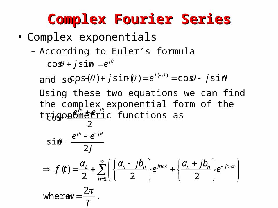
dvevfFdeF
dedvevftf
T
vjtj
tj
v
vj
)(2
1)( where)(
2
1
)(2
1
2
1)(
integralan become sum the, As
These two integrals form the conclusion of Fourier’s integral theorem.

Alternative FormsAlternative Forms
• Note that there are a number of alternative forms for Fourier transform, such as
– The third form is popular in the field of signal processing and communications systems.
dtetfuFdueuFtf
u
dtetfFdeFtf
dtetfFdeFtf
utjutj
tjtj
tjtj
22 )()( where)()(
2 definingby lexponentia in the 2 theabsorbingby or,
)()( where)(2
1)(
)(2
1)( where)()(
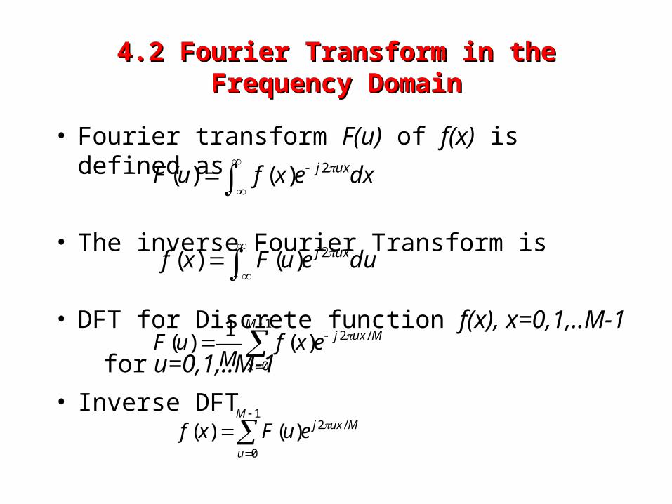
4.2 Fourier Transform in the4.2 Fourier Transform in theFrequency DomainFrequency Domain
• Fourier transform F(u) of f(x) is defined as
• The inverse Fourier Transform is
• DFT for Discrete function f(x), x=0,1,..M-1
for u=0,1,..M-1
• Inverse DFT
dxexfuF uxj 2)()(
dueuFxf uxj 2)()(
1
0
/2)(1
)(M
x
MuxjexfM
uF
1
0
/2)()(M
u
MuxjeuFxf

• Euler’s formula:
• Each term of the Fourier transform is composed of the sum of all values of the function f(x).– M2 summations and multiplications– The values of f(x) are multiplied by sines and cosines
of various frequencies.– The domain (values of u) over which the values of
F(u) range is appropriately called the frequency domain, because u determines the frequency of the components of the transform.
– Each of the M terms of F(u) is called a frequency component of the transform.
1.,2,.. ,1,0 for
]/2sin/2)[cos(1
)(1
0
Mu
MuxjMuxxfM
uFM
x
sincos je j
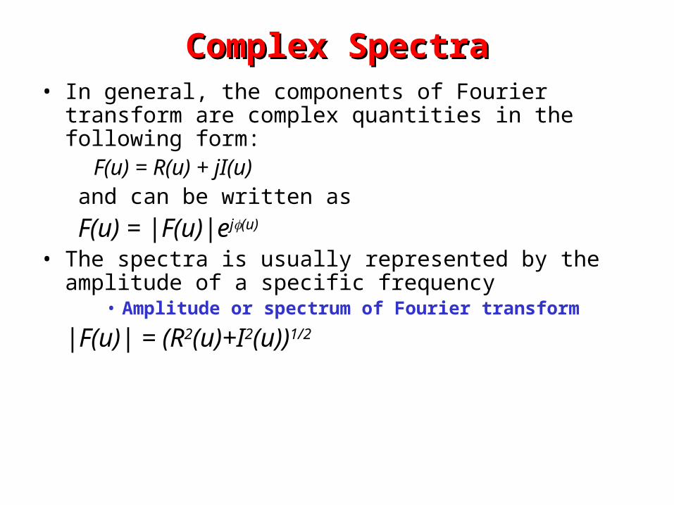
Complex SpectraComplex Spectra• In general, the components of Fourier transform are complex
quantities in the following form:F(u) = R(u) + jI(u)
and can be written as
F(u) = |F(u)|ej(u)
• The spectra is usually represented by the amplitude of a specific frequency
• Amplitude or spectrum of Fourier transform
|F(u)| = (R2(u)+I2(u))1/2
Complex SpectraComplex Spectra
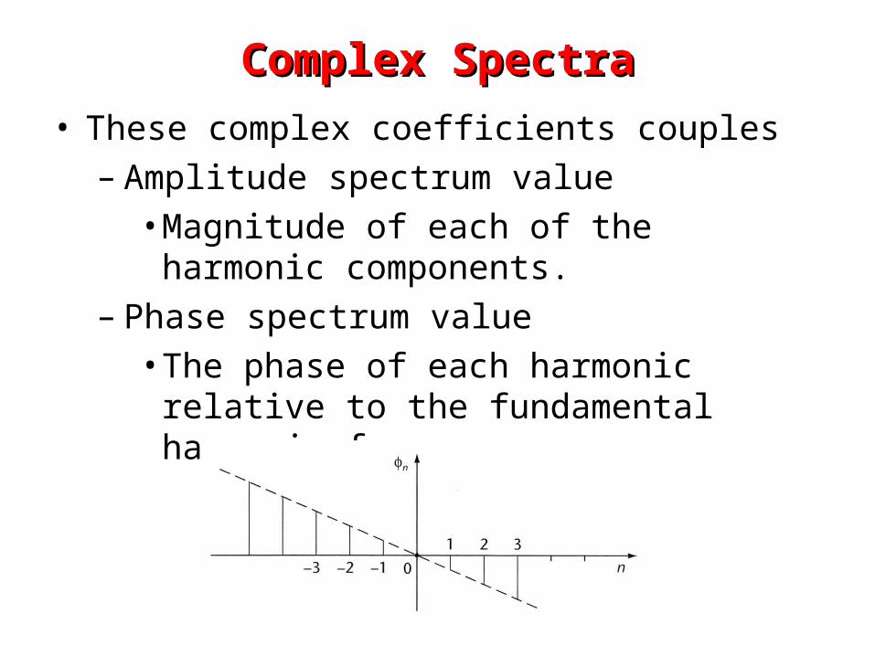
• These complex coefficients couples – Amplitude spectrum value
• Magnitude of each of the harmonic components.
– Phase spectrum value • The phase of each harmonic relative to the
fundamental harmonic frequency ω0.

The frequency spectrum is centered at 0. To visual easily, we sometimes multiply f(x) by (-1)x before applying the transform.

Why (-1)Why (-1)xx??
)2
()(1
)(1
)(1
)()1(1
)()sin(cos)1(
1
0
/)2
(2
1
0
/2
1
0
/2
1
0
/2
MuFexf
M
exfM
exfeM
exfM
eej
M
x
MM
uxj
M
x
Muxjxj
M
x
Muxjxj
M
x
Muxjx
xjxjxx
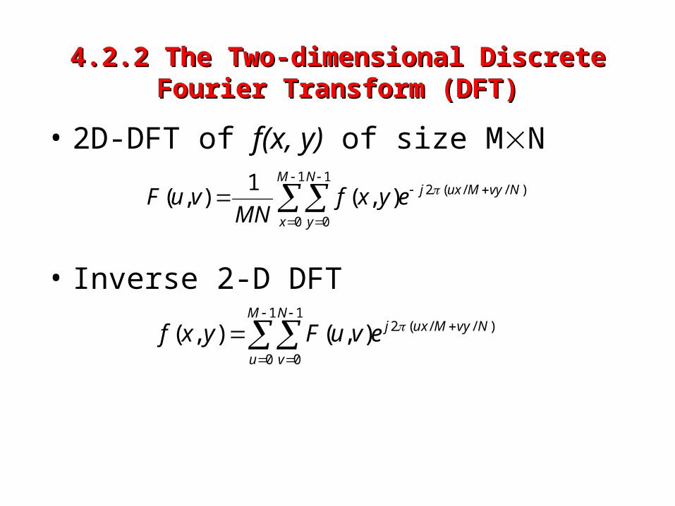
4.2.2 The Two-dimensional Discrete Fourier 4.2.2 The Two-dimensional Discrete Fourier Transform (DFT)Transform (DFT)
• 2D-DFT of f(x, y) of size MN
• Inverse 2-D DFT
1
0
1
0
)//(2),(1
),(M
x
N
y
NvyMuxjeyxfMN
vuF
1
0
1
0
)//(2),(),(M
u
N
v
NvyMuxjevuFyxf

• Modulation in the space domain F[(-1)x+yf(x, y)]= F(u-M/2,v-N/2)
• Shift the origin of F(u,v) to frequency coordinates (M/2, N/2),– the center of (u, v), u=0,…M-1, v=0,…N-1.– frequency rectangle
• Average of f(x,y)
• For real f(x,y)F(u, v) = F*(-u, -v)|F(u, v)| = |F(-u, -v)|
– The spectrum of the Fourier transform is symmetric.
1M
0x
1N
0y
yxfMN
1)0,0F( ),(

ImplementationImplementation

• What is the “frequency” of an image?– Since frequency is directly related rate of
change, it is not difficult intuitively to associate frequencies with pattern of intensity variations in an image.
• The low frequencies correspond to the slowly varying components of an image.
• The higher frequencies begin to correspond to faster and faster gray level changes in the image.
– such as edges.
– F(0, 0): the average gray level of an image.
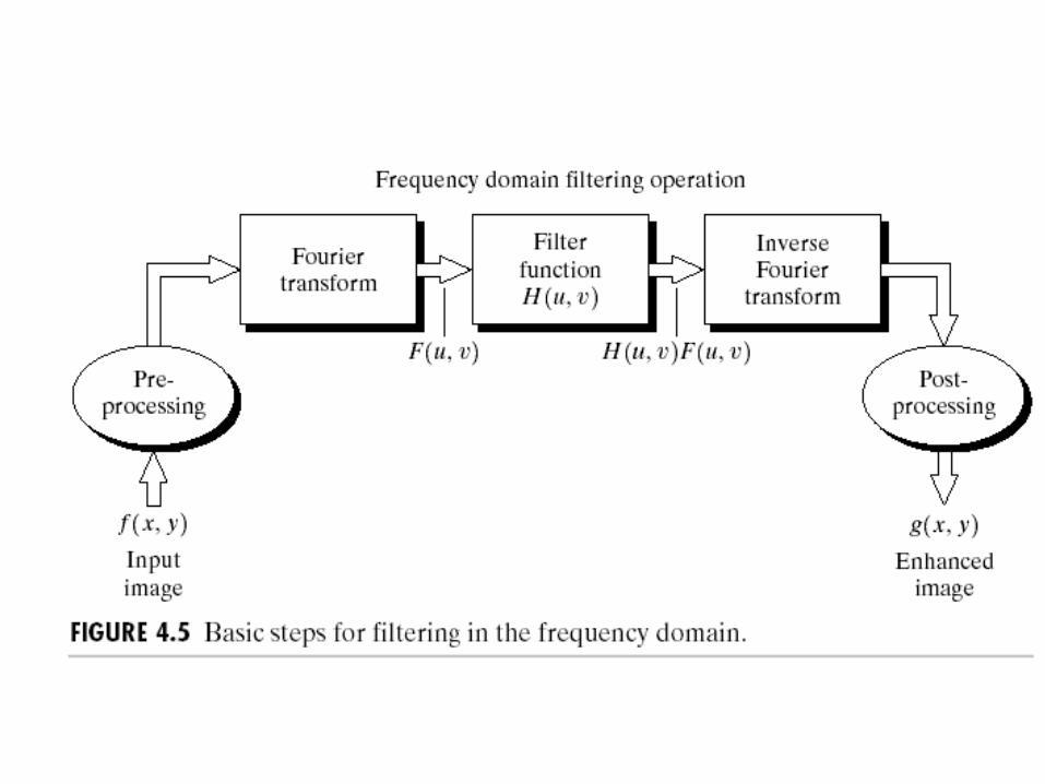
4.2.3 Filtering in the Frequency Domain4.2.3 Filtering in the Frequency Domain4.2.3 Filtering in the Frequency Domain4.2.3 Filtering in the Frequency Domain


1) Multiply the input image by (-1)x+y to center the transform.
2) Compute DFT F(u, v)
3) Multiply F(u,v) by a filter function H(u,v)
G(u,v) = F(u,v)H(u,v)
4) Computer the inverse DFT of G(u,v)
5) Obtain the real part of g(x,y)
6) Multiply g(x,y) with (-1)x+y
Filtering steps:

Notch filter: H(u,v) = 0 if (u,v) = (M/2, N/2), H(u,v) = 1 otherwise
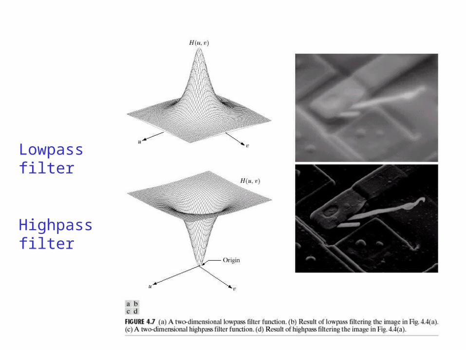
Lowpass filter
Highpass filter

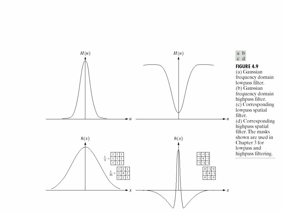
4.2.4 Filtering in 4.2.4 Filtering in spatialspatial and frequency domains and frequency domains
• The discrete convolution f(x,y)*h(x,y)
• f(x,y)*h(x,y) F(u,v)H(u,v)• f(x,y)h(x,y) F(u,v)*H(u,v)
1M
0m
1N
0n
nymxhnmfMN
1yxhy)xf ),(),(),(,(
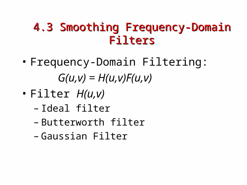
4.3 Smoothing Frequency-Domain Filters4.3 Smoothing Frequency-Domain Filters
• Frequency-Domain Filtering:
G(u,v) = H(u,v)F(u,v)
• Filter H(u,v)– Ideal filter– Butterworth filter– Gaussian Filter

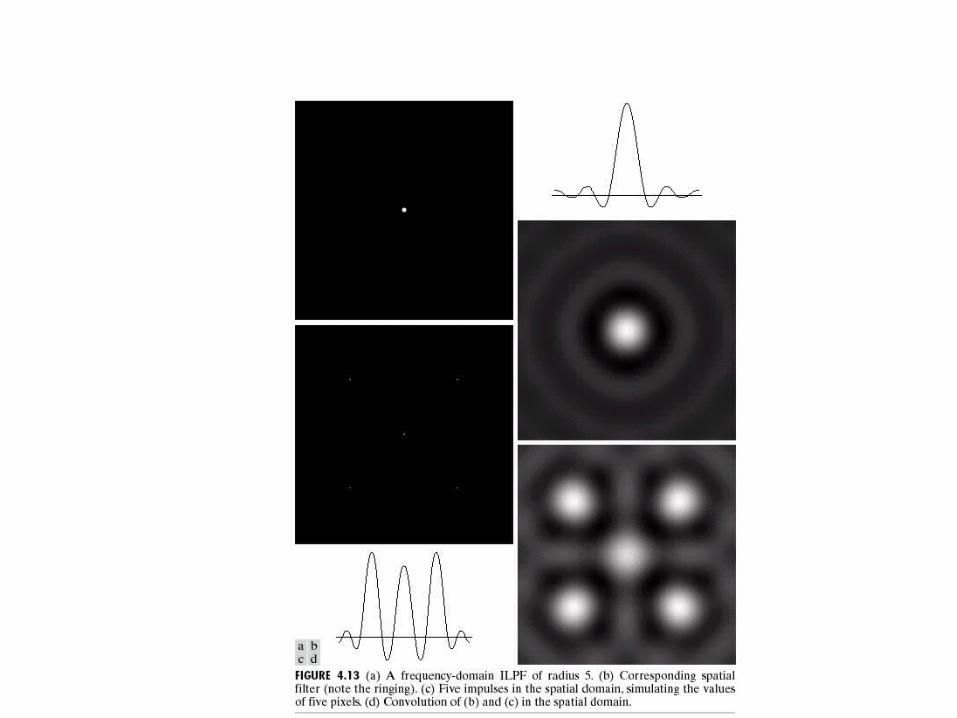
4.3.1 Ideal Low pass filter4.3.1 Ideal Low pass filter
• H(u,v) = 1 if D(u,v) D0
= 0 if D(u,v) > D0
• The center is at (u,v)=(M/2, N/2)
D(u,v)=[(u-M/2)2 + (v-N/2)2]1/2
• Cutoff frequency is D0
• Power estimate:The percentage α of power enclosed in the circle is:
1
0
1
0
),( where,/),(100M
u
N
vT
u vT vuPPPvuP


•The blurring in this image is a clear indication that most of the sharp detail information in the picture is contained in the 8% power removed by the filter.
•The result of α =99.5 is quite close to the original, indicating little edge information is contained in the upper 0.5% of the spectrum power.

4.3.2 Butterworth Lowpass Filter
• Butterworth lowpass filter (BLPF) of order n
• At the frequency as an half of the cutoff frequency D0, H(u, v)=0.5.
nDvuDvuH
20 ]/),([1
1),(

4.3.2 Butterworth Lowpass Filter4.3.2 Butterworth Lowpass Filter

4.3.2 Butterworth Lowpass Filter4.3.2 Butterworth Lowpass Filter

4.3.2 Butterworth Lowpass Filter4.3.2 Butterworth Lowpass Filter

4.3.3 Gaussian Lowpass Filter
• Gaussian filter
• Let =D0
• When D(u, v)=D0 , H(u, v)=0.667
22 2/),(),( vuDevuH
20
2 2/),(),( DvuDevuH

4.3.3 Gaussian Lowpass Filter4.3.3 Gaussian Lowpass Filter

4.3.3 Gaussian Lowpass Filter4.3.3 Gaussian Lowpass Filter
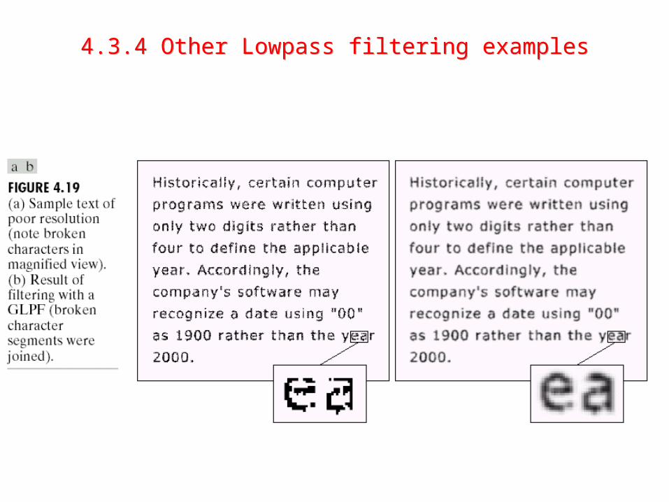
4.3.4 Other Lowpass filtering examples4.3.4 Other Lowpass filtering examples
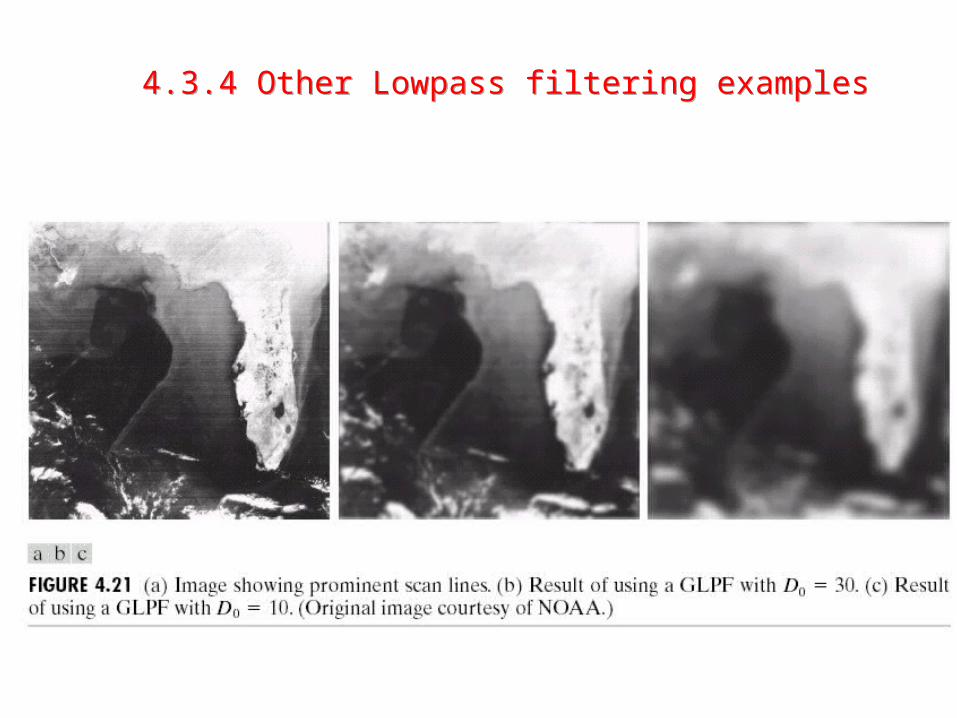
4.3.4 Other Lowpass filtering examples4.3.4 Other Lowpass filtering examples
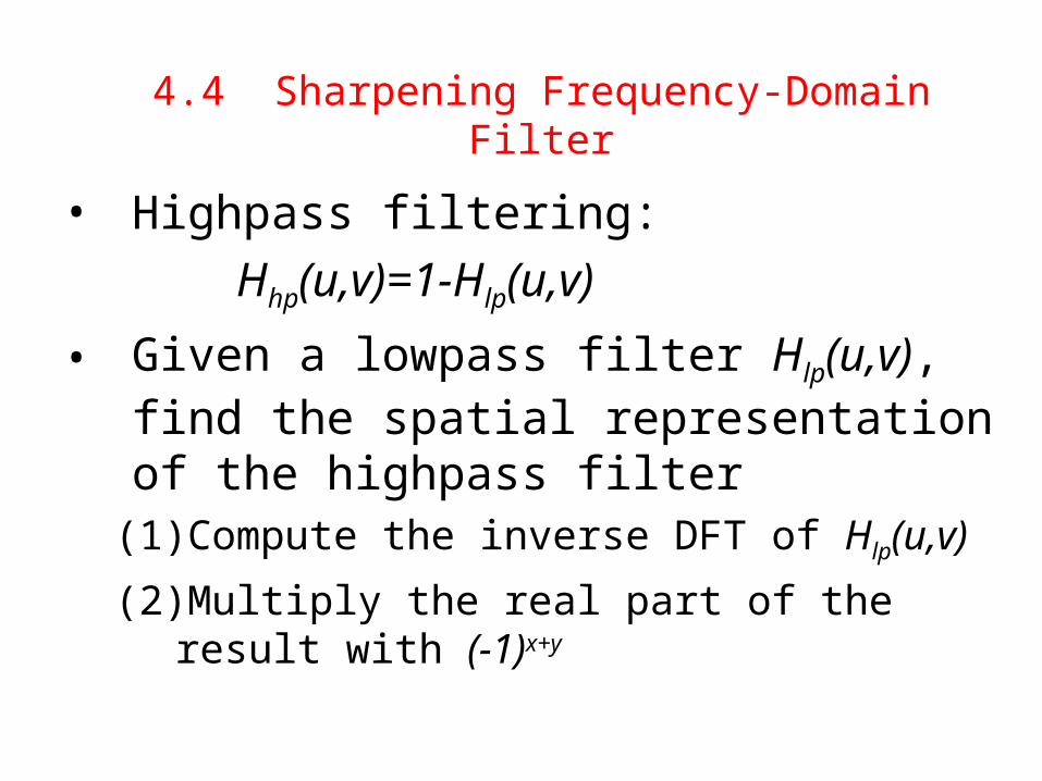
4.4 Sharpening Frequency-Domain Filter
• Highpass filtering:
Hhp(u,v)=1-Hlp(u,v)
• Given a lowpass filter Hlp(u,v), find the spatial representation of the highpass filter
(1) Compute the inverse DFT of Hlp(u,v)
(2) Multiply the real part of the result with (-1)x+y

4.4 Sharpening Frequency-Domain Filter 4.4 Sharpening Frequency-Domain Filter

4.4 Sharpening Frequency-Domain Filter4.4 Sharpening Frequency-Domain Filter

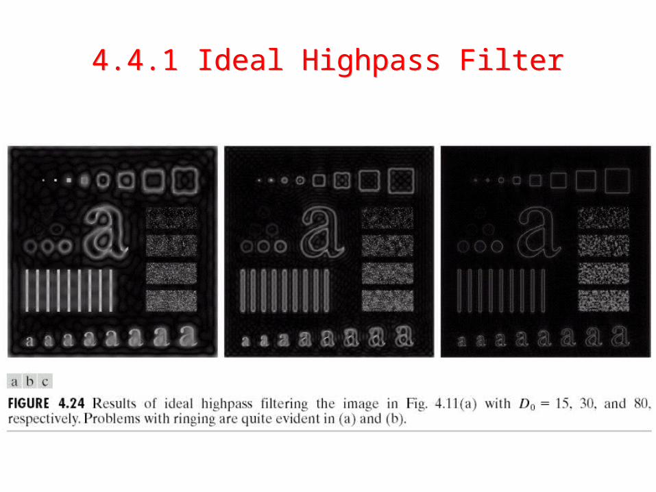
4.4.1 Ideal Highpass Filter
• H(u,v)=0 if D(u,v)D0
=1 if D(u,v)>D0
• The center is at (u,v)=(M/2, N/2)
D(u,v)=[(u-M/2)2+(v-N/2)2]1/2
• Cutoff frequency is D0
4.4.1 Ideal Highpass Filter4.4.1 Ideal Highpass Filter

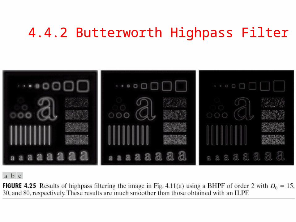
4.4.2 Butterworth Highpass Filter
• Butterworth filter has no sharp cutoff
• At cutoff frequency D0: H(u, v)=0.5
nvuDDvuH
20 )],(/[1
1),(
4.4.2 Butterworth Highpass Filter4.4.2 Butterworth Highpass Filter
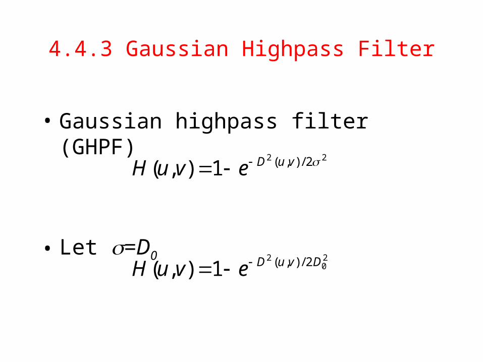
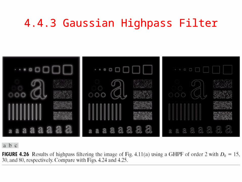
4.4.3 Gaussian Highpass Filter
• Gaussian highpass filter (GHPF)
• Let =D0
22 2/),(1),( vuDevuH
20
2 2/),(1),( DvuDevuH
4.4.3 Gaussian Highpass Filter4.4.3 Gaussian Highpass Filter
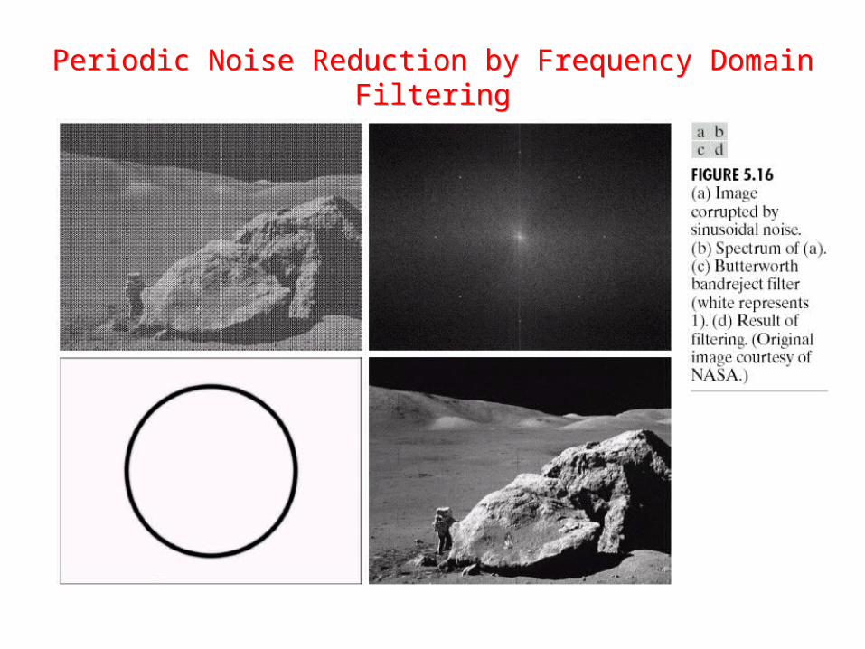
5.4 Periodic Noise Reduction by Frequency Domain Filtering
• Periodic noise is due to the electrical or electromechanical interference during image acquisition.
• Can be estimated through the inspection of the Fourier spectrum of the image.
Periodic Noise Reduction by Frequency Domain FilteringPeriodic Noise Reduction by Frequency Domain Filtering

5.4 Periodic Noise Reduction by Frequency Domain Filtering
• Bandreject filters– Remove or attenuate a band of frequencies.
• D0 is the radius.
• D(u, v) is the distance from the origin, and
• W is the width of the frequency band.
2/),(
2/),(2/
2/),(
1
0
1
),(
0
00
0
WDvuDif
WDvuDWDif
WDvuDif
vuH
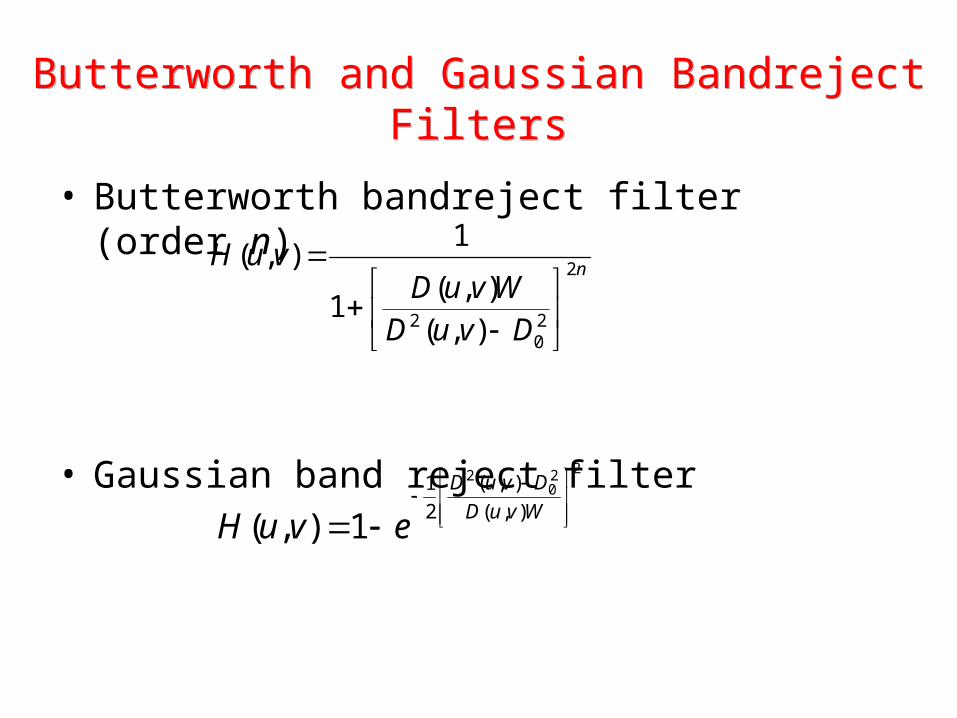
• Butterworth bandreject filter (order n)
• Gaussian band reject filter
n
DvuDWvuD
vuH 2
20
2 ),(),(
1
1),(
Butterworth and Gaussian Bandreject FiltersButterworth and Gaussian Bandreject Filters
220
2
),(
),(
2
1
1),(
WvuD
DvuD
evuH

Bandreject FiltersBandreject Filters

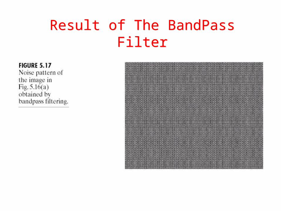
Bandpass filter
• Obtained form bandreject filter
Hbp(u,v)=1-Hbr(u,v)
• The goal of the bandpass filter is to isolate the noise pattern from the original image, which can help simplify the analysis of noise, reasonably independent of image content.
Result of The BandPass FilterResult of The BandPass Filter

5.4.3 Notch filters
• Notch filter rejects (passes) frequencies in predefined neighborhoods about a center frequency.
where
otherwise
DvuDorDvuDifvuH
1
),(),(0),( 0201
2/120
201 )2/()2/(),( vNvuMuvuD
2/120
202 )2/()2/(),( vNvuMuvuD

• Butterworth notch filter
• Gaussian notch filter
• Note that these notch filters will become highpass when u0=v0=0
n
vuDvuDD
vuH
),(),(1
1),(
21
20
20
21 ),(),(
2
1
1),( D
vuDvuD
evuH
5.4.3 Notch filters
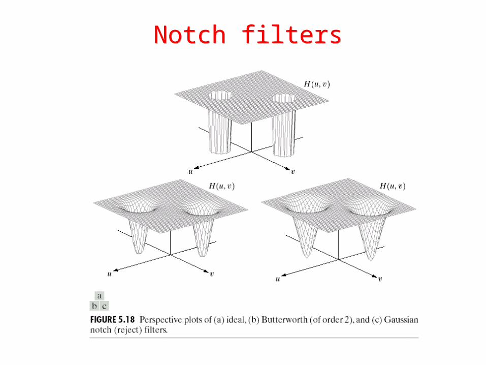
Notch filtersNotch filters
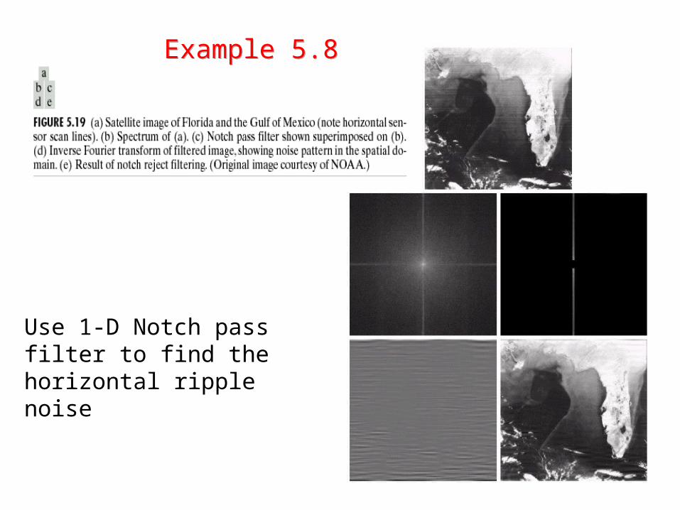
Example 5.8Example 5.8
Use 1-D Notch pass filter to find the horizontal ripple noise
Recommended