Copyright ©2012 Pearson Education, Inc. publishing as Prentice Hall Chap 15-1Chap 15-1
Chapter 15
Multiple Regression Model Building
Basic Business Statistics12th Edition
Chap 15-2Copyright ©2012 Pearson Education, Inc. publishing as Prentice Hall Chap 15-2
Learning Objectives
In this chapter, you learn: To use quadratic terms in a regression model To use transformed variables in a regression
model To measure the correlation among the
independent variables To build a regression model using either the
stepwise or best-subsets approach To avoid the pitfalls involved in developing a
multiple regression model
Chap 15-3Copyright ©2012 Pearson Education, Inc. publishing as Prentice Hall Chap 15-3
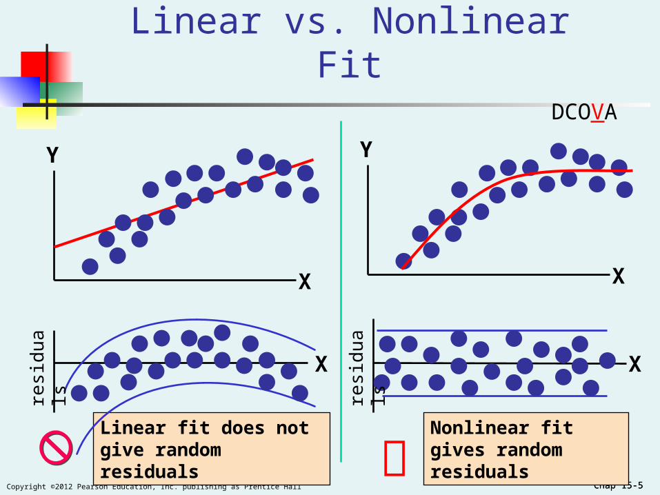
The relationship between the dependent variable and an independent variable may not be linear
Can review the scatter plot to check for non-linear relationships
Example: Quadratic model
The second independent variable is the square of the first variable
Nonlinear Relationships
i21i21i10i εXβXββY
DCOVA
Chap 15-4Copyright ©2012 Pearson Education, Inc. publishing as Prentice Hall Chap 15-4
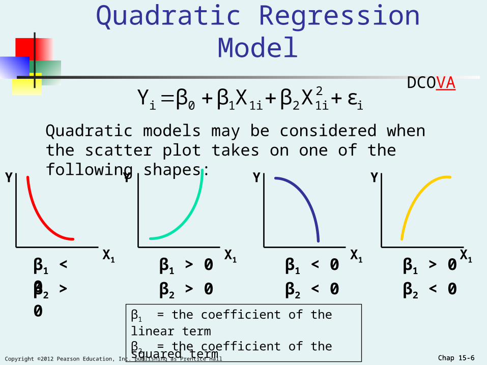
Quadratic Regression Model
where:
β0 = Y intercept
β1 = regression coefficient for linear effect of X on Y
β2 = regression coefficient for quadratic effect on Y
εi = random error in Y for observation i
i21i21i10i εXβXββY
Model form:DCOVA
Chap 15-5Copyright ©2012 Pearson Education, Inc. publishing as Prentice Hall Chap 15-5
Linear fit does not give random residuals
Linear vs. Nonlinear Fit
Nonlinear fit gives random residuals
X
resi
dua
ls
X
Y
X
resi
dua
ls
Y
X
DCOVA
Chap 15-6Copyright ©2012 Pearson Education, Inc. publishing as Prentice Hall Chap 15-6
Quadratic Regression Model
Quadratic models may be considered when the scatter plot takes on one of the following shapes:
X1
Y
X1X1
YYY
β1 < 0 β1 > 0 β1 < 0 β1 > 0
β1 = the coefficient of the linear term
β2 = the coefficient of the squared term
X1
i21i21i10i εXβXββY
β2 > 0 β2 > 0 β2 < 0 β2 < 0
DCOVA
Chap 15-7Copyright ©2012 Pearson Education, Inc. publishing as Prentice Hall Chap 15-7
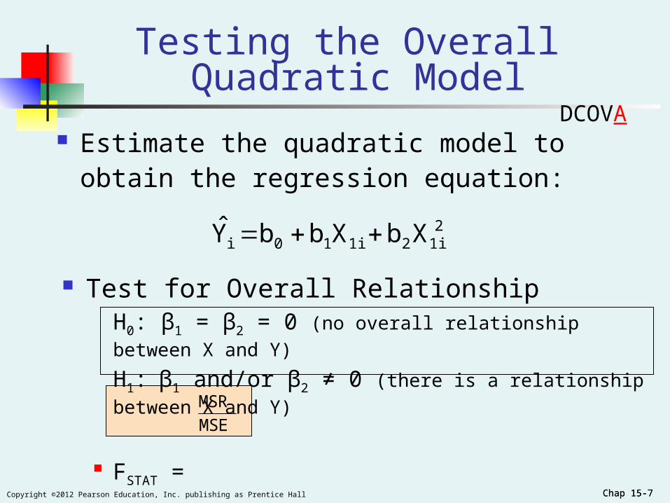
Testing the Overall Quadratic Model
Test for Overall RelationshipH0: β1 = β2 = 0 (no overall relationship between X and Y)
H1: β1 and/or β2 ≠ 0 (there is a relationship between X and Y)
FSTAT =
2 1i21i10i XbXbbY
MSE
MSR
Estimate the quadratic model to obtain the regression equation:
DCOVA
Chap 15-8Copyright ©2012 Pearson Education, Inc. publishing as Prentice Hall Chap 15-8
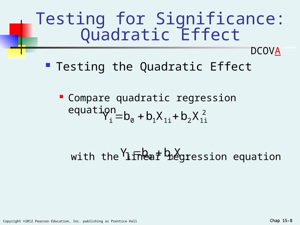
Testing for Significance: Quadratic Effect
Testing the Quadratic Effect
Compare quadratic regression equation
with the linear regression equation
2 1i21i10i XbXbbY
1i10i XbbY
DCOVA
Chap 15-9Copyright ©2012 Pearson Education, Inc. publishing as Prentice Hall Chap 15-9
Testing for Significance: Quadratic Effect
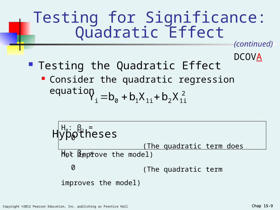
Testing the Quadratic Effect Consider the quadratic regression equation
Hypotheses (The quadratic term does not improve the model)
(The quadratic term improves the model)
2 1i21i10i XbXbbY
H0: β2 = 0
H1: β2 0
(continued)
DCOVA
Chap 15-10Copyright ©2012 Pearson Education, Inc. publishing as Prentice Hall Chap 15-10
Testing for Significance: Quadratic Effect
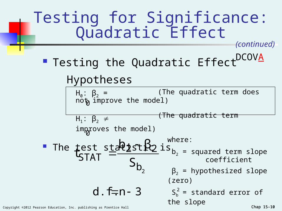
Testing the Quadratic Effect
Hypotheses (The quadratic term does not improve the model)
(The quadratic term improves the model)
The test statistic is
H0: β2 = 0
H1: β2 0
(continued)
2b
22STAT S
βbt
3nd.f.
where:
b2 = squared term slope coefficient
β2 = hypothesized slope (zero)
Sb = standard error of the slope2
DCOVA
Chap 15-11Copyright ©2012 Pearson Education, Inc. publishing as Prentice Hall Chap 15-11
Testing for Significance: Quadratic Effect
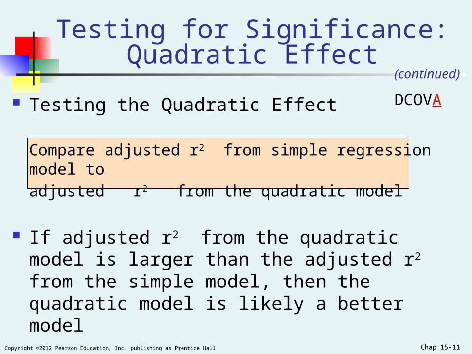
Testing the Quadratic Effect
Compare adjusted r2 from simple regression model to
adjusted r2 from the quadratic model
If adjusted r2 from the quadratic model is larger than the adjusted r2 from the simple model, then the quadratic model is likely a better model
(continued)
DCOVA
Chap 15-12Copyright ©2012 Pearson Education, Inc. publishing as Prentice Hall Chap 15-12
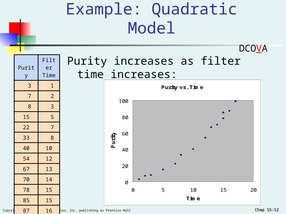
Example: Quadratic Model
Purity increases as filter time increases:PurityFilterTime
3 1
7 2
8 3
15 5
22 7
33 8
40 10
54 12
67 13
70 14
78 15
85 15
87 16
99 17
Purity vs. Time
0
20
40
60
80
100
0 5 10 15 20
Time
Pu
rity
DCOVA
Chap 15-13Copyright ©2012 Pearson Education, Inc. publishing as Prentice Hall Chap 15-13
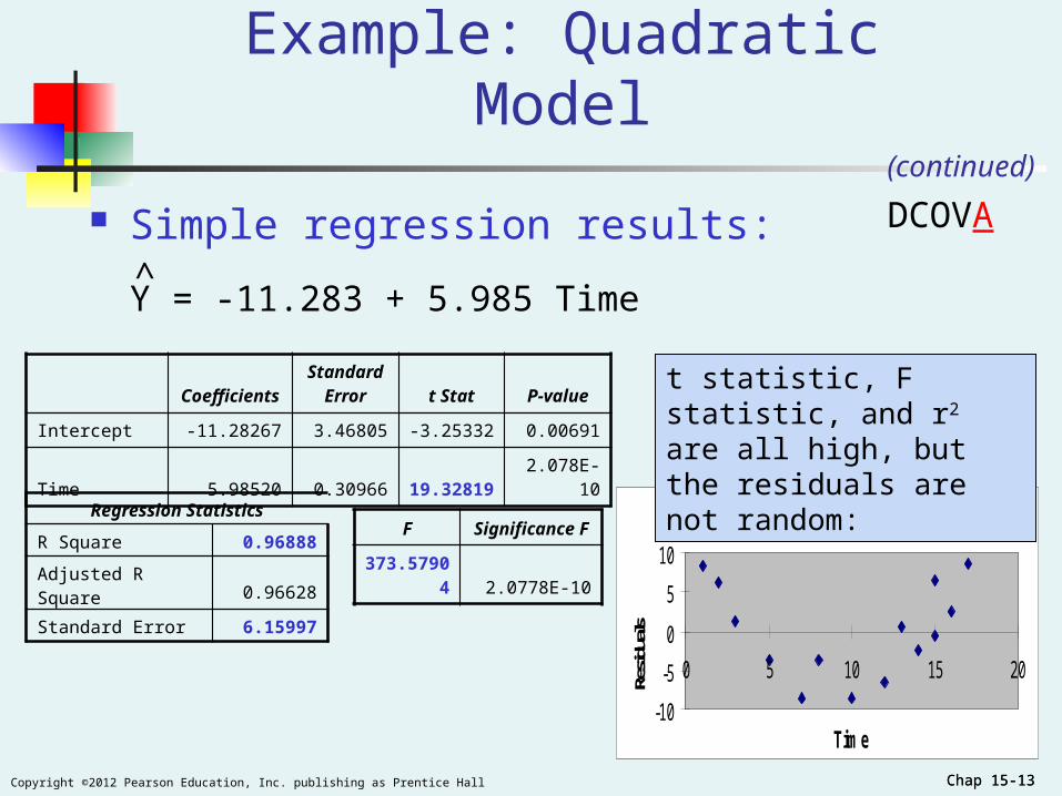
Example: Quadratic Model(continued)
Regression Statistics
R Square 0.96888
Adjusted R Square 0.96628
Standard Error 6.15997
Simple regression results:
Y = -11.283 + 5.985 Time
CoefficientsStandard
Error t Stat P-value
Intercept -11.28267 3.46805 -3.25332 0.00691
Time 5.98520 0.30966 19.32819 2.078E-10
FSignificance
F
373.57904 2.0778E-10
^
Time Residual Plot
-10
-5
0
5
10
0 5 10 15 20
Time
Resid
uals
t statistic, F statistic, and r2 are all high, but the residuals are not random:
DCOVA
Chap 15-14Copyright ©2012 Pearson Education, Inc. publishing as Prentice Hall Chap 15-14
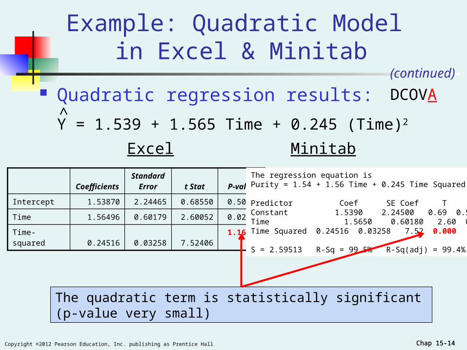
CoefficientsStandard
Error t Stat P-value
Intercept 1.53870 2.24465 0.68550 0.50722
Time 1.56496 0.60179 2.60052 0.02467
Time-squared 0.24516 0.03258 7.52406 1.165E-05
Quadratic regression results:
Y = 1.539 + 1.565 Time + 0.245 (Time)2^
Example: Quadratic Model in Excel & Minitab
(continued)
The quadratic term is statistically significant (p-value very small)
DCOVA
The regression equation isPurity = 1.54 + 1.56 Time + 0.245 Time Squared Predictor Coef SE Coef T PConstant 1.5390 2.24500 0.69 0.507Time 1.5650 0.60180 2.60 0.025Time Squared 0.24516 0.03258 7.52 0.000 S = 2.59513 R-Sq = 99.5% R-Sq(adj) = 99.4%
Excel Minitab
Chap 15-15Copyright ©2012 Pearson Education, Inc. publishing as Prentice Hall Chap 15-15
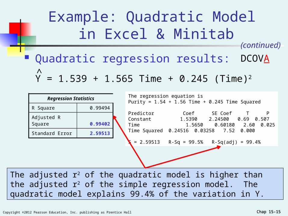
Regression Statistics
R Square 0.99494
Adjusted R Square 0.99402
Standard Error 2.59513
Quadratic regression results:
Y = 1.539 + 1.565 Time + 0.245 (Time)2^
Example: Quadratic Model in Excel & Minitab
(continued)
The adjusted r2 of the quadratic model is higher than the adjusted r2 of the simple regression model. The quadratic model explains 99.4% of the variation in Y.
DCOVA
The regression equation isPurity = 1.54 + 1.56 Time + 0.245 Time Squared Predictor Coef SE Coef T PConstant 1.5390 2.24500 0.69 0.507Time 1.5650 0.60180 2.60 0.025Time Squared 0.24516 0.03258 7.52 0.000 S = 2.59513 R-Sq = 99.5% R-Sq(adj) = 99.4%
Chap 15-16Copyright ©2012 Pearson Education, Inc. publishing as Prentice Hall
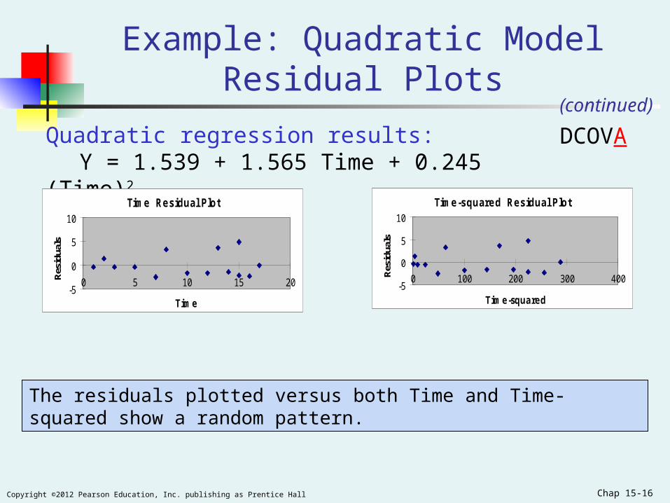
Example: Quadratic Model Residual Plots
Quadratic regression results:Y = 1.539 + 1.565 Time + 0.245 (Time)2
The residuals plotted versus both Time and Time-squared show a random pattern.
Time Residual Plot
-5
0
5
10
0 5 10 15 20
Time
Res
idua
ls
Time-squared Residual Plot
-5
0
5
10
0 100 200 300 400
Time-squared
Res
idua
ls
(continued)
DCOVA
Chap 15-17Copyright ©2012 Pearson Education, Inc. publishing as Prentice Hall Chap 15-17
Using Transformations in Regression Analysis
Idea: non-linear models can often be transformed
to a linear form Can be estimated by least squares if transformed
transform X or Y or both to get a better fit or to deal with violations of regression assumptions
Can be based on theory, logic or scatter plots
DCOVA
Chap 15-18Copyright ©2012 Pearson Education, Inc. publishing as Prentice Hall Chap 15-18
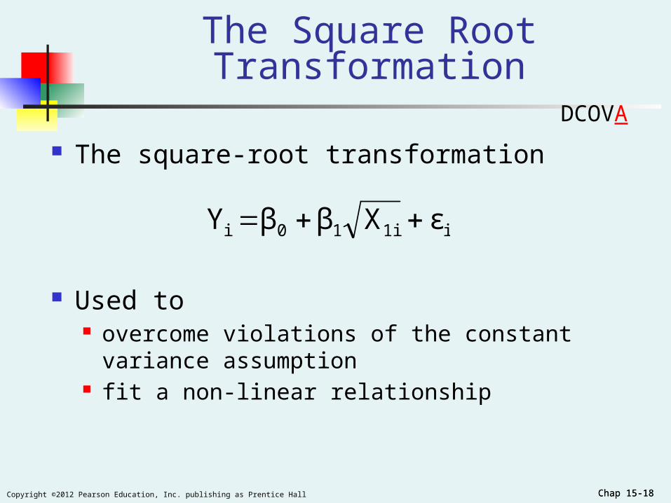
The Square Root Transformation
The square-root transformation
Used to overcome violations of the constant variance
assumption fit a non-linear relationship
i1i10i εXββY
DCOVA
Chap 15-19Copyright ©2012 Pearson Education, Inc. publishing as Prentice Hall Chap 15-19
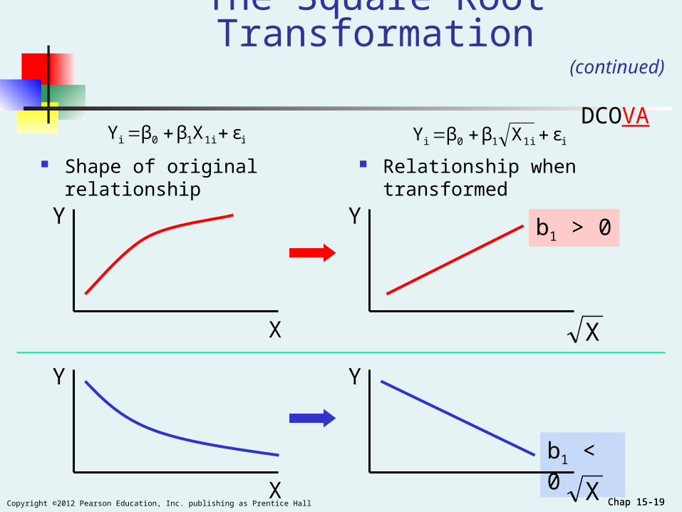
Shape of original relationship
X
The Square Root Transformation(continued)
b1 > 0
b1 < 0
X
Y
Y
Y
Y
X
X
Relationship when transformed
i1i10i εXββY i1i10i εXββY DCOVA
Chap 15-20Copyright ©2012 Pearson Education, Inc. publishing as Prentice Hall Chap 15-20
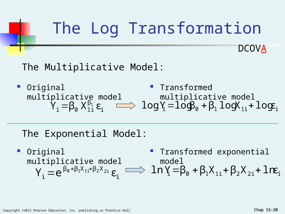
Original multiplicative model
The Log Transformation
Transformed multiplicative model
iβ1i0i εXβY 1 i1i10i ε logX log ββ log Ylog
The Multiplicative Model:
Original multiplicative model Transformed exponential model
i2i21i10i ε ln XβXββ Yln
The Exponential Model:
iXβXββ
i εeY 2i21i10
DCOVA
Chap 15-21Copyright ©2012 Pearson Education, Inc. publishing as Prentice Hall Chap 15-21
Interpretation of Coefficients
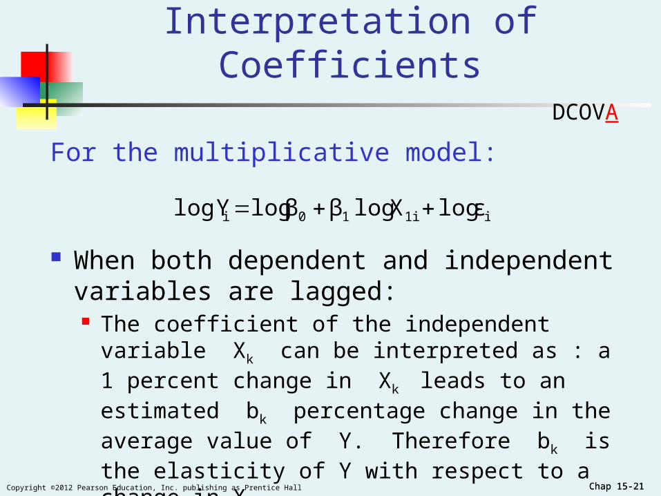
For the multiplicative model:
When both dependent and independent variables are lagged: The coefficient of the independent variable Xk can
be interpreted as : a 1 percent change in Xk leads to an estimated bk percentage change in the average value of Y. Therefore bk is the elasticity of Y with respect to a change in Xk .
i1i10i ε logX log ββ log Ylog
DCOVA
Chap 15-22Copyright ©2012 Pearson Education, Inc. publishing as Prentice Hall Chap 15-22
Collinearity
Collinearity: High correlation exists among two or more independent variables
This means the correlated variables contribute redundant information to the multiple regression model
DCOVA
Chap 15-23Copyright ©2012 Pearson Education, Inc. publishing as Prentice Hall Chap 15-23
Collinearity
Including two highly correlated independent variables can adversely affect the regression results
No new information provided
Can lead to unstable coefficients (large standard error and low t-values)
Coefficient signs may not match prior expectations
(continued)
DCOVA
Chap 15-24Copyright ©2012 Pearson Education, Inc. publishing as Prentice Hall Chap 15-24
Some Indications of Strong Collinearity
Incorrect signs on the coefficients Large change in the value of a previous
coefficient when a new variable is added to the model
A previously significant variable becomes non-significant when a new independent variable is added
The estimate of the standard deviation of the model increases when a variable is added to the model
DCOVA
Chap 15-25Copyright ©2012 Pearson Education, Inc. publishing as Prentice Hall Chap 15-25
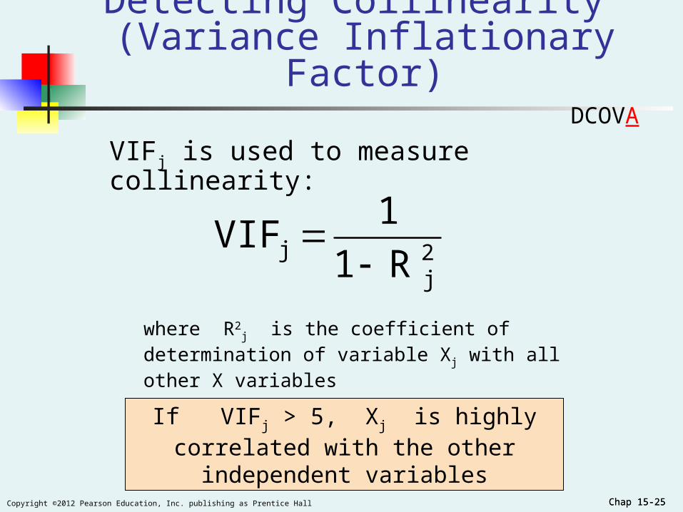
Detecting Collinearity (Variance Inflationary Factor)
VIFj is used to measure collinearity:
If VIFj > 5, Xj is highly correlated with the other independent variables
where R2j is the coefficient of determination of
variable Xj with all other X variables
2j
j R1
1VIF
DCOVA
Chap 15-26Copyright ©2012 Pearson Education, Inc. publishing as Prentice Hall Chap 15-26
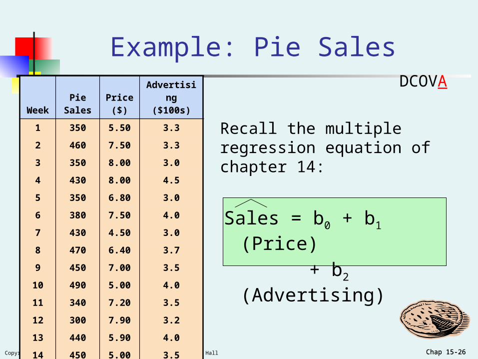
Example: Pie Sales
Sales = b0 + b1 (Price)
+ b2 (Advertising)
WeekPie
SalesPrice
($)Advertising
($100s)
1 350 5.50 3.3
2 460 7.50 3.3
3 350 8.00 3.0
4 430 8.00 4.5
5 350 6.80 3.0
6 380 7.50 4.0
7 430 4.50 3.0
8 470 6.40 3.7
9 450 7.00 3.5
10 490 5.00 4.0
11 340 7.20 3.5
12 300 7.90 3.2
13 440 5.90 4.0
14 450 5.00 3.5
15 300 7.00 2.7
Recall the multiple regression equation of chapter 14:
DCOVA
Chap 15-27Copyright ©2012 Pearson Education, Inc. publishing as Prentice Hall Chap 15-27
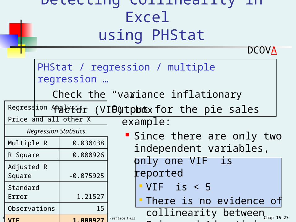
Detecting Collinearity in Excel using PHStat
Output for the pie sales example: Since there are only two
independent variables, only one VIF is reported
VIF is < 5 There is no evidence of
collinearity between Price and Advertising
Regression Analysis
Price and all other X
Regression Statistics
Multiple R 0.030438
R Square 0.000926
Adjusted R Square -0.075925
Standard Error 1.21527
Observations 15
VIF 1.000927
PHStat / regression / multiple regression …
Check the “variance inflationary factor (VIF)” box
DCOVA
Chap 15-28Copyright ©2012 Pearson Education, Inc. publishing as Prentice Hall Chap 15-28
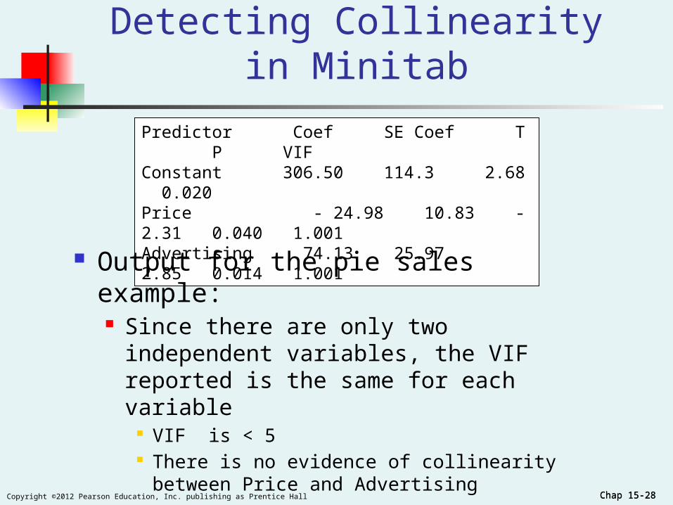
Detecting Collinearity in Minitab
Predictor Coef SE Coef T P VIFConstant 306.50 114.3 2.68 0.020Price - 24.98 10.83 -2.31 0.040 1.001Advertising 74.13 25.97 2.85 0.014 1.001
Output for the pie sales example: Since there are only two independent
variables, the VIF reported is the same for each variable
VIF is < 5 There is no evidence of collinearity between Price
and Advertising
Chap 15-29Copyright ©2012 Pearson Education, Inc. publishing as Prentice Hall Chap 15-29
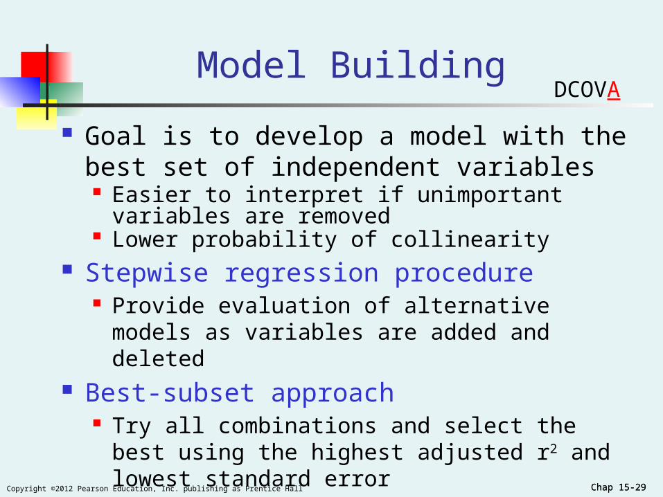
Model Building
Goal is to develop a model with the best set of independent variables Easier to interpret if unimportant variables are
removed Lower probability of collinearity
Stepwise regression procedure Provide evaluation of alternative models as variables
are added and deleted Best-subset approach
Try all combinations and select the best using the highest adjusted r2 and lowest standard error
DCOVA
Chap 15-30Copyright ©2012 Pearson Education, Inc. publishing as Prentice Hall Chap 15-30
Idea: develop the least squares regression equation in steps, adding one independent variable at a time and evaluating whether existing variables should remain or be removed
The coefficient of partial determination is the measure of the marginal contribution of each independent variable, given that other independent variables are in the model
Stepwise RegressionDCOVA
Chap 15-31Copyright ©2012 Pearson Education, Inc. publishing as Prentice Hall Chap 15-31
Best Subsets Regression
Idea: estimate all possible regression equations using all possible combinations of independent variables
Choose the best fit by looking for the highest adjusted r2 and lowest standard error
Stepwise regression and best subsets regression can be performed using PHStat
DCOVA
Chap 15-32Copyright ©2012 Pearson Education, Inc. publishing as Prentice Hall Chap 15-32
Alternative Best Subsets Criterion
Calculate the value Cp for each potential regression model
Consider models with Cp values close to or below k + 1
k is the number of independent variables in the model under consideration
DCOVA
Chap 15-33Copyright ©2012 Pearson Education, Inc. publishing as Prentice Hall Chap 15-33
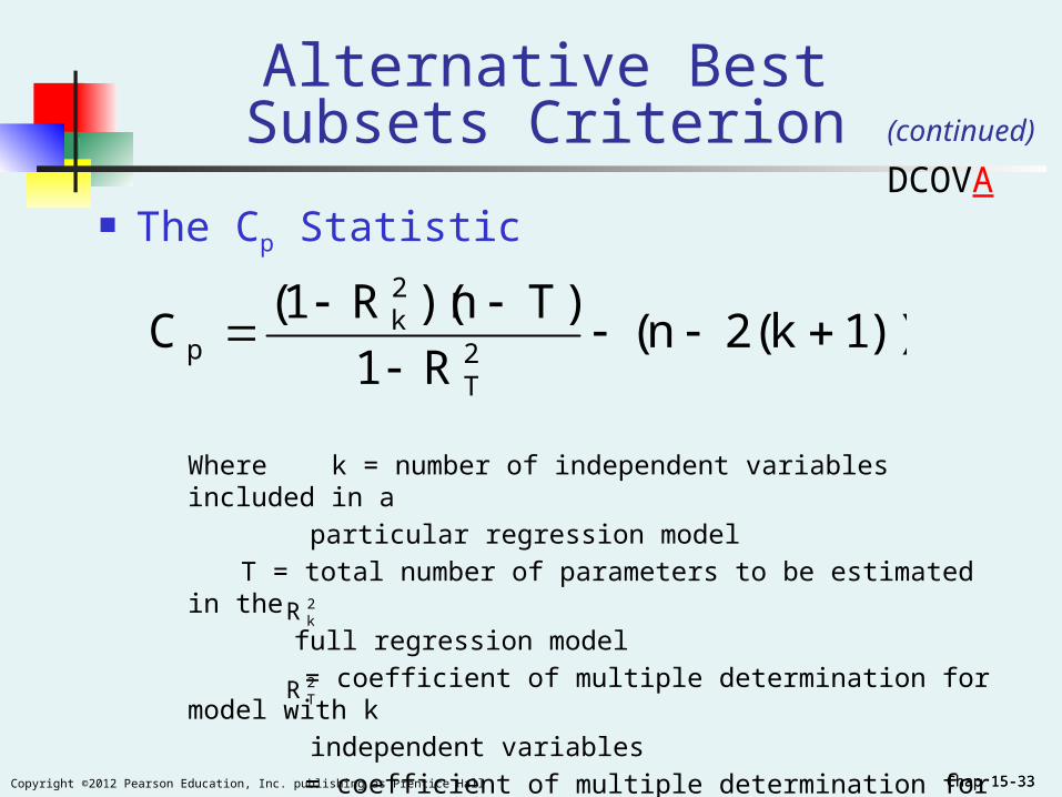
Alternative Best Subsets Criterion
The Cp Statistic
))1k(2n(R1
)Tn)(R1(C
2T
2k
p
Where k = number of independent variables included in a
particular regression model
T = total number of parameters to be estimated in the
full regression model
= coefficient of multiple determination for model with k
independent variables
= coefficient of multiple determination for full model with
all T estimated parameters
2kR
2TR
(continued)
DCOVA
Chap 15-34Copyright ©2012 Pearson Education, Inc. publishing as Prentice Hall Chap 15-34
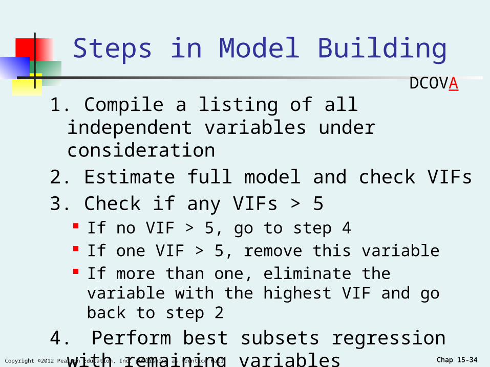
Steps in Model Building
1. Compile a listing of all independent variables under consideration
2. Estimate full model and check VIFs
3. Check if any VIFs > 5 If no VIF > 5, go to step 4 If one VIF > 5, remove this variable If more than one, eliminate the variable with the
highest VIF and go back to step 2
4.Perform best subsets regression with remaining variables
DCOVA
Chap 15-35Copyright ©2012 Pearson Education, Inc. publishing as Prentice Hall Chap 15-35
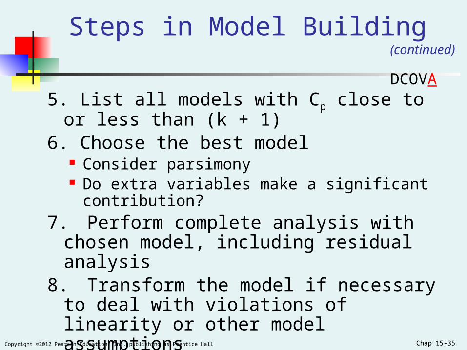
Steps in Model Building
5. List all models with Cp close to or less than (k + 1)
6. Choose the best model Consider parsimony Do extra variables make a significant contribution?
7.Perform complete analysis with chosen model, including residual analysis
8.Transform the model if necessary to deal with violations of linearity or other model assumptions
9.Use the model for prediction and inference
(continued)
DCOVA
Chap 15-36Copyright ©2012 Pearson Education, Inc. publishing as Prentice Hall Chap 15-36
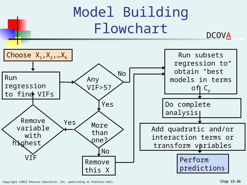
Model Building Flowchart
Choose X1,X2,…Xk
Run regression to find VIFs
Remove variable with
highest VIF
Any VIF>5?
Run subsets regression to obtain
“best” models in terms of Cp
Do complete analysis
Add quadratic and/or interaction terms or transform variables
Perform predictions
No
More than one?
Remove this X
Yes
No
Yes
DCOVA
Chap 15-37Copyright ©2012 Pearson Education, Inc. publishing as Prentice Hall Chap 15-37
Pitfalls and Ethical Considerations
Understand that interpretation of the estimated regression coefficients are performed holding all other independent variables constant
Evaluate residual plots for each independent variable
Evaluate interaction terms
To avoid pitfalls and address ethical considerations:
Chap 15-38Copyright ©2012 Pearson Education, Inc. publishing as Prentice Hall Chap 15-38
Additional Pitfalls and Ethical Considerations
Obtain VIFs for each independent variable before determining which variables should be included in the model
Examine several alternative models using best-subsets regression
Use other methods when the assumptions necessary for least-squares regression have been seriously violated
To avoid pitfalls and address ethical considerations:
(continued)
Chap 15-39Copyright ©2012 Pearson Education, Inc. publishing as Prentice Hall Chap 15-39
Chapter Summary
Developed the quadratic regression model Discussed using transformations in
regression models The multiplicative model The exponential model
Described collinearity Discussed model building
Stepwise regression Best subsets
Addressed pitfalls in multiple regression and ethical considerations
Copyright ©2012 Pearson Education, Inc. publishing as Prentice Hall Chap 15-40
On-Line Topic
Influence Analysis
Basic Business Statistics12th Edition
Chap 15-41Copyright ©2012 Pearson Education, Inc. publishing as Prentice Hall
Learning Objective
To learn how to measure the influence of individual observations using: The hat matrix elements hi
The Studentized deleted residuals ti
Cook’s distance statistic Di
Chap 15-42Copyright ©2012 Pearson Education, Inc. publishing as Prentice Hall
Influence Analysis Helps Identify Individual Observations Having A Disproportionate Impact On The Analysis
There are three commonly used measures of influence: The diagonal values of the hat matrix hi
The Studentized deleted residuals ti
Cook’s distance statistic Di
Each of these measure influence in slightly different ways.
If potentially influential observations are present you may want to delete them and redo the analysis.
DCOVA
Chap 15-43Copyright ©2012 Pearson Education, Inc. publishing as Prentice Hall
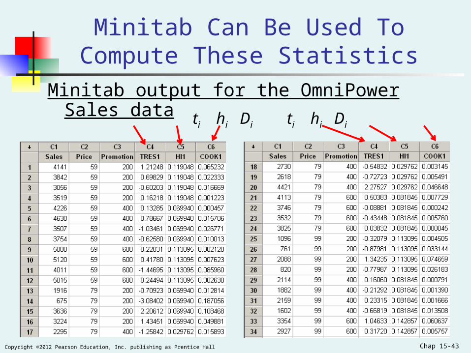
Minitab Can Be Used To Compute These Statistics
Minitab output for the OmniPower Sales data
ti hi Di ti hi Di
Chap 15-44Copyright ©2012 Pearson Education, Inc. publishing as Prentice Hall
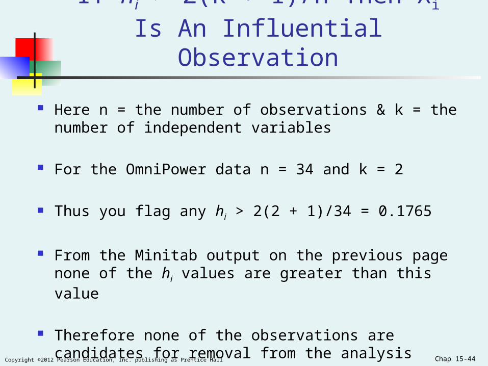
If hi > 2(k + 1)/n Then Xi Is An Influential Observation
Here n = the number of observations & k = the number of independent variables
For the OmniPower data n = 34 and k = 2
Thus you flag any hi > 2(2 + 1)/34 = 0.1765
From the Minitab output on the previous page none of the hi values are greater than this value
Therefore none of the observations are candidates for removal from the analysis
Chap 15-45Copyright ©2012 Pearson Education, Inc. publishing as Prentice Hall
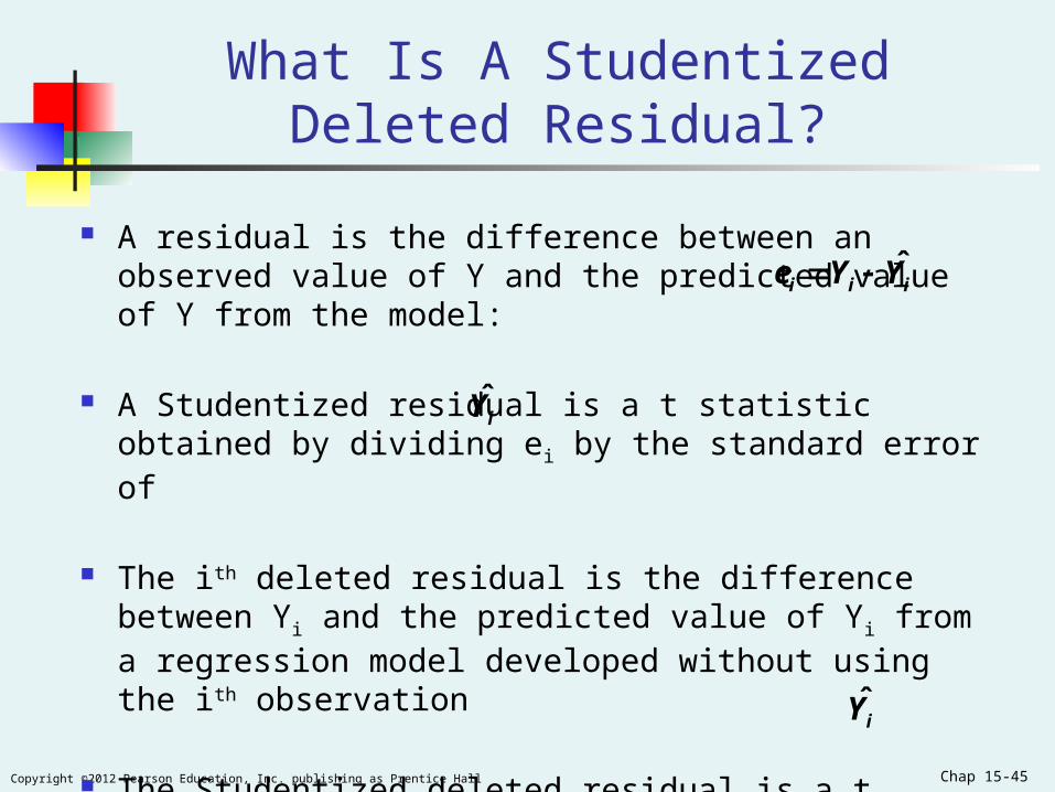
What Is A Studentized Deleted Residual?
A residual is the difference between an observed value of Y and the predicted value of Y from the model:
A Studentized residual is a t statistic obtained by dividing e i by the standard error of
The ith deleted residual is the difference between Yi and the predicted value of Yi from a regression model developed without using the ith observation
The Studentized deleted residual is a t statistic obtained by dividing a deleted residual by the standard error of
iii YYe ˆ
iY
iY
Chap 15-46Copyright ©2012 Pearson Education, Inc. publishing as Prentice Hall
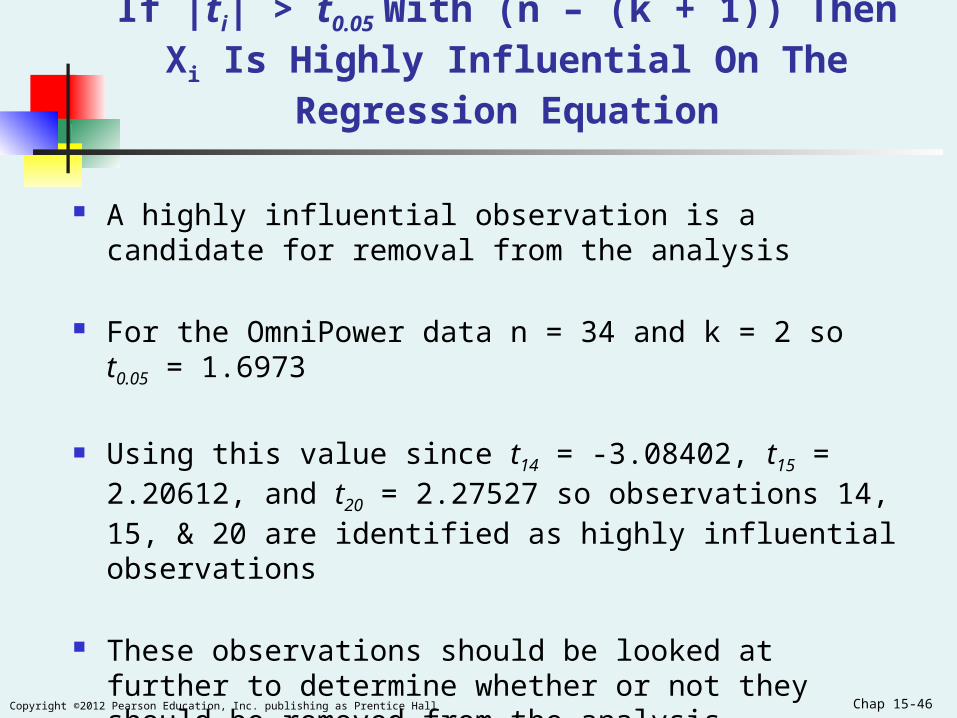
If |ti| > t0.05 With (n – (k + 1)) Then Xi Is Highly Influential On The Regression Equation
A highly influential observation is a candidate for removal from the analysis
For the OmniPower data n = 34 and k = 2 so t0.05 = 1.6973
Using this value since t14 = -3.08402, t15 = 2.20612, and t20 = 2.27527 so observations 14, 15, & 20 are identified as highly influential observations
These observations should be looked at further to determine whether or not they should be removed from the analysis
Chap 15-47Copyright ©2012 Pearson Education, Inc. publishing as Prentice Hall
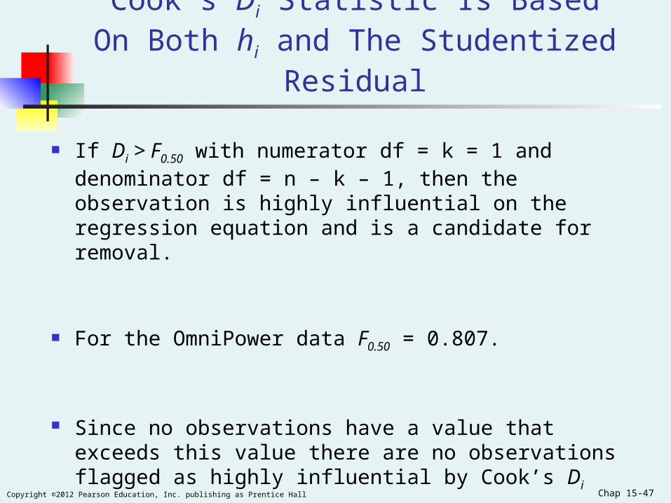
Cook’s Di Statistic Is Based On Both hi and The Studentized Residual
If Di > F0.50 with numerator df = k = 1 and denominator df = n – k – 1, then the observation is highly influential on the regression equation and is a candidate for removal.
For the OmniPower data F0.50 = 0.807.
Since no observations have a value that exceeds this value there are no observations flagged as highly influential by Cook’s Di
Chap 15-48Copyright ©2012 Pearson Education, Inc. publishing as Prentice Hall
Topic Summary
Discussed how to measure the influence of individual observations using: The hat matrix elements hi
The Studentized deleted residuals ti
Cook’s distance statistic Di
Copyright ©2012 Pearson Education, Inc. publishing as Prentice Hall Chap 15-49
On-Line Topic
Analytics & Data Mining
Basic Business Statistics12th Edition
Chap 15-50Copyright ©2012 Pearson Education, Inc. publishing as Prentice Hall
Learning Objective
To develop an awareness of the topic of data mining and what it is being used for in business today
Chap 15-51Copyright ©2012 Pearson Education, Inc. publishing as Prentice Hall
Data Mining Is A Sophisticated Quantitative Analysis That Attempts To Discover Useful Patterns Or Relationships In
A Group Of Data
Some examples of data mining in use today are: Mortgage acceptance & default -- predicting which applicants
will qualify for a specific type of mortgage Retention -- who will remain a customer of the financial
services company Response to promotions -- predicting who will respond to
promotions Purchasing associations -- predicting what product a
consumer will purchase given that they have purchased another product
Product failure -- Predicting the type of product that will fail during a warranty period
DCOVA
Chap 15-52Copyright ©2012 Pearson Education, Inc. publishing as Prentice Hall
Data Mining Typically Involves The Analysis Of Very Large Data Sets
Large data sets have many observations and many variables
Working with such data sets increases the importance of how data is collected so that it can be readily analyzed to arrive at useful conclusions
Chap 15-53Copyright ©2012 Pearson Education, Inc. publishing as Prentice Hall
Data Mining Can be Divided Into Two Types Of Tasks
Exploratory Data Analysis Examining the basic features of a data set via
Tables, Descriptive Statistics, & Graphic Displays
Predictive Modeling Building a model to predict a variable based on the
value of other variables via Simple Linear Regression, Multiple Regression Model
Building, Stepwise Regression, & Logistic Regression
Chap 15-54Copyright ©2012 Pearson Education, Inc. publishing as Prentice Hall
Data Mining Also Uses Other Methods Not Discussed In This Book
Classification & Regression Trees (CART)
Chi-square Automatic Interaction Dectector (CHAID)
Neural Nets
Cluster Analysis
Multidimensional Scaling
Chap 15-55Copyright ©2012 Pearson Education, Inc. publishing as Prentice Hall
Topic Summary
Introduced the topic of data mining and discussed the vast array of statistical techniques used.
Recommended