Statistical Inference
Part II: Confidence IntervalPart II: Confidence Interval

In addition to the estimated value of the estimator, some statisticians suggest that we should also consider the variance of the estimatorvariance of the estimator.
Use the single value and the variance of the estimator to form an interval that has a high probability to cover the unknown parameter.
Thi th d i l di th i f th i tThis method including the variance of the point estimator is called interval estimation, or " fid i t l""confidence interval".

Interval estimationInterval estimationAssume that and are two functions of a random sample and areLθ̂ Uθ̂Assume that and are two functions of a random sample and are determined by a point estimator of an unknown parameter such that
Lθ Uθθ̂ θ
ˆˆ αθθθ −=≤≤ 1)ˆˆ( ULPwhere αα is a known value between is a known value between 0 and 10 and 1.
Interval estimationInterval estimation
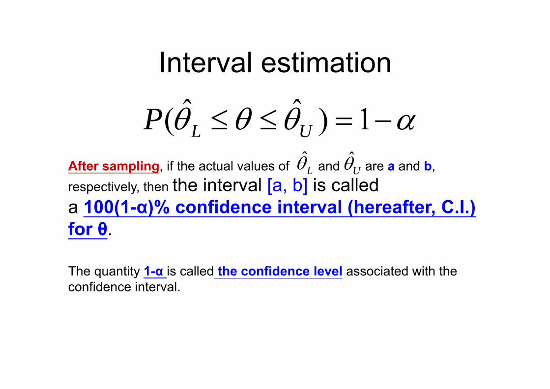
ˆˆ αθθθ −=≤≤ 1)( ULPAfter sampling, if the actual values of and are a and b, respectively, then the interval [a, b] is called
Lθ̂ Uθ̂[ ]
a 100(1-α)% confidence interval (hereafter, C.I.) for θ.
The quantity 1-α is called the confidence level associated with the fid i t lconfidence interval.

Caution:Caution:By the definition, before samplingbefore sampling, we have a random interval estimationinterval estimation
]ˆ,ˆ[ UL θθ ],[ ULfor the unknown parameter θ.
After samplingAfter sampling, the confidence interval [a, b] is a fixed (not random) interval and depends on the particular sample ) p p pobservations we collect.

Caution:Caution:Most importantly, the unknown parameter θ is either inside or outside the confidence interval [a b] That isor outside the confidence interval [a, b].That is,
P(a ≤ θ ≤ b) = 0 or 1.( )After sampling, we have observations nxx ,,1 K
],[ ba⇒P(a ≤ θ ≤ b) = 0
[ [
P(a ≤ θ ≤ b) = 0
θ[ [
a b

Caution:Caution:Most importantly, the unknown parameter θ is either inside or outside the confidence interval [a b] That isor outside the confidence interval [a, b].That is,
P(a ≤ θ ≤ b) = 0 or 1.( )After sampling, we have observations nxx ,,1 K
],[ ba⇒P(a ≤ θ ≤ b) = 1
[ [
P(a ≤ θ ≤ b) 1
θ[ [
a b

Caution:Caution:Most importantly, the unknown parameter θ is either inside or outside the confidence interval [a b] That isor outside the confidence interval [a, b].That is,
P(a ≤ θ ≤ b) = 0 or 1.( )
Recall that before sampling we haveRecall that before sampling, we have
αθθθ =≤≤ 1)ˆˆ(P αθθθ −=≤≤ 1)( ULP

Interpretation of C.I.The interpretation of a 100(1-α)% C I is that when we
pThe interpretation of a 100(1-α)% C.I. is that when we obtained N (sufficient large) independent sets of random sample and for each set of random sample, we construct p pone particular interval by using the same point estimator, then there are N(1-α) out of these N intervals will contain th t k t θthe true unknown parameter θ.
However we do not know which interval will contain θ andHowever, we do not know which interval will contain θ and which will not contain θ, because θ is unknown.

Interpretation of C.I.pFor instance, if we construct a random interval by drawing o sta ce, e co st uct a a do te a by d a gdifferent sets of samples repeatedly, say 100 times, then
95% = 100(1-0 05)% C I for μ means that μ is contained in95% = 100(1-0.05)% C.I. for μ means that μ is contained in 95 out of the 100 fixed intervals. Again, we do not know what these 95 intervals are, because µ is unknown., µ
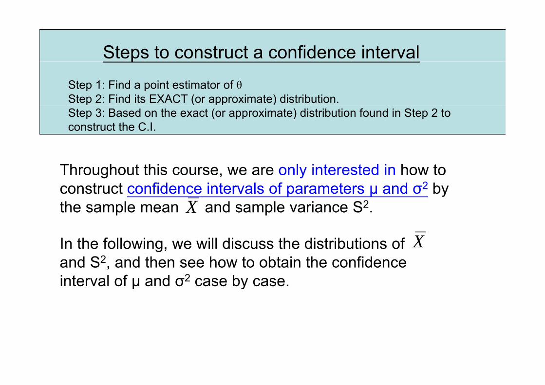
Steps to construct a confidence interval
Step 1: Find a point estimator of θStep 2: Find its EXACT (or approximate) distribution.
p
( )Step 3: Based on the exact (or approximate) distribution found in Step 2 to construct the C.I.
Throughout this course, we are only interested in how to construct confidence intervals of parameters µ and σ2 byconstruct confidence intervals of parameters µ and σ by the sample mean and sample variance S2. X
XIn the following, we will discuss the distributions ofand S2, and then see how to obtain the confidence interval of µ and σ2 case by case
X
interval of µ and σ2 case by case.
One sample
Confidence Interval for µ withConfidence Interval for µ with NORMAL population
(k i )(known variance)

Confidence interval for µConfidence interval for µCase I: Normal distribution with unknown mean and KNOWNKNOWN variancevariance:Case o a d st but o t u o ea a d OO a a cea a ce
Consider a random sample of size n, {X1, X2, …, Xn}, from a normal distribution with unknown mean µ and KNOWNKNOWN variance σ2. That is,
.),(~,, 21 σμNXX nK
Then we have a result that the sampling distribution of the sample mean is
)(2
NX σ ),(~n
NX σμOr equivalently
)1,0(~)( NXnZ μ−=
Or equivalently,
),(σ
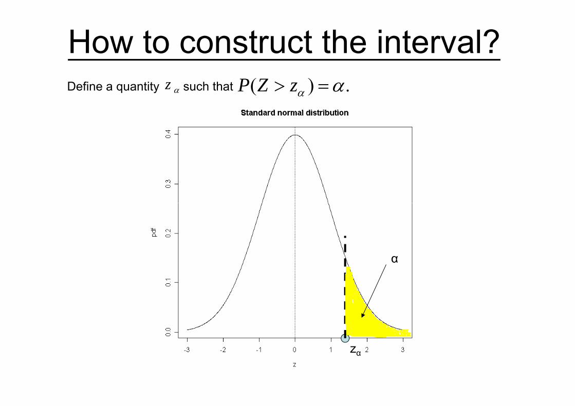
How to construct the interval?αzDefine a quantity such that .)( αα => zZP
α
zα

How to construct the interval?αzDefine a quantity such that .)( αα => zZP
μ≤
−≤ 1))(( XnP
By the symmetry of the standard normal distribution, we have
ασ
μαα −=≤≤− 1))(( 2/2/ zzP

How to construct the interval?))(
σμ−
=XnZ
z1-α/2
σ
1 α/2
= -zα/2
α/2α/21 - α
zα/2

How to construct the interval?αzDefine a quantity such that .)( αα => zZP
μ≤
−≤ 1))(( XnP
By the symmetry of the standard normal distribution, we haveθ
ασ
μαα −=≤≤− 1))(( 2/2/ zzP
σσ 2/2/ zzLθ̂
Uθ̂ασμσ αα −=+≤≤− 1)( 2/2/
nzX
nzXP

How to construct the interval?xAfter sampling, we can find an actual value of the sample mean, say . Thus,
100(1-α)% C.I for μ is that
⎥⎤
⎢⎡ +−
zxzx σσ αα 2/2/ , ⎥⎦⎢⎣+
nx
nx ,
or simply written as
zx σα 2/± The margin of error
nx ± The margin of error
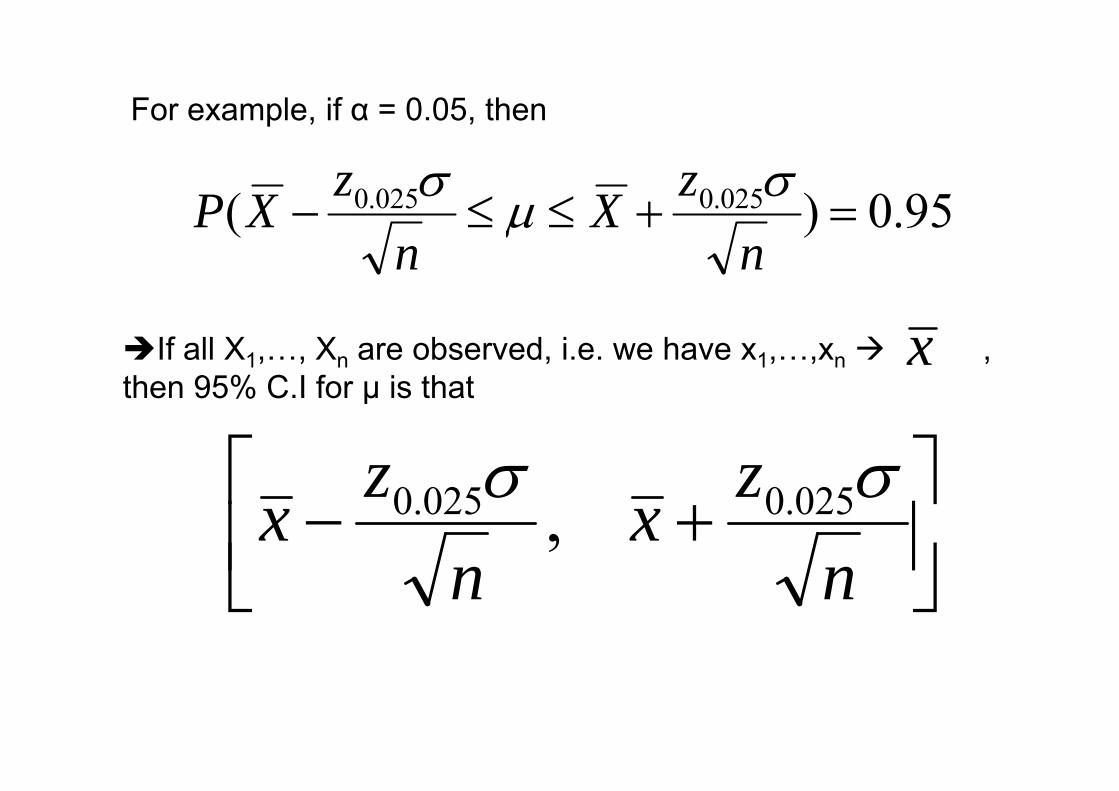
For example, if α = 0.05, then
950)( 025.0025.0 =+≤≤−zXzXP σμσ
p
95.0)( =+≤≤n
Xn
XP μ
xIf all X1,…, Xn are observed, i.e. we have x1,…,xn , then 95% C.I for μ is thatthen 95% C.I for μ is that
⎤⎡ zz σσ⎥⎦
⎤⎢⎣
⎡ +−n
zxn
zx σσ 025.0025.0 ,⎦⎣ nn

Remark again that it does not mean that μ is inside this interval with a probability 0 95this interval with a probability 0.95. Note that μ is an unknown BUT fixed number, and and σ2
kx
So, μ is either inside or outside the fixed interval.are known.
10)( 025.0025.0 orzxzxP =+≤≤−σμσ
nn
95.0)( 025.0025.0 =+≤≤−n
zXn
zXP σμσ

One sample
Confidence Interval for µ withConfidence Interval for µ with NORMAL population ( k i )(unknown variance)

Confidence interval for µConfidence interval for µCase II: Normal distribution with unknown mean and UNKNOWNUNKNOWN variancevariance:Case o a d st but o t u o ea a d U OU O a a cea a ce
Consider a random sample of size n, {X1, X2, …, Xn}, from a normal distribution with unknown mean µ and UNKNOWNUNKNOWN variance σ2. That is,
.),(~,, 21 σμNXX nK
Then we have a result that the sampling distribution of the sample mean is
)(2
NX σ ),(~n
NX σμOr equivalently
)1,0(~)( NXnZ μ−=
Or equivalently,
),(σ
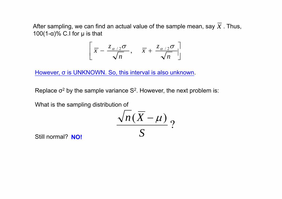
xAfter sampling, we can find an actual value of the sample mean, say . Thus, 100(1 )% C I f i th t
⎥⎦
⎤⎢⎣
⎡ +−zxzx σσ αα 2/2/ ,
100(1-α)% C.I for μ is that
⎥⎦⎢⎣ nn
However, σ is UNKNOWN. So, this interval is also unknown.
Replace σ2 by the sample variance S2. However, the next problem is:
?)(Xn μ−What is the sampling distribution of
?)(S
μStill normal? NO!

C id d l f i {X X X } f l
TheoremConsider a random sample of size n, {X1, X2, …, Xn}, from a normal distribution with unknown mean µ and UNKNOWN variance σ2.
Then the sampling distribution ofThen the sampling distribution of
Xn )( μ−S
has a Student t distribution (or simply t distribution) with n -1 degrees of freedom. D t bDenote by
11 ~)( −= tXnT μ
11 −− nn tS
T
∑n
XX 1 ∑n
XXS 22 )(1∑=
=i
iXn
X1
1 ∑=
−−
=i
i XXn
S1
22 )(11
where and

tk distribution
• Similar to a standard normal distribution it is also symmetric about 0 so• Similar to a standard normal distribution, it is also symmetric about 0, so
P(T ≤ -a) = 1 - P(T ≤ a) = P(T ≥ a), if T follows a t distribution.
• Use a table of a t distribution to find a probability of a t-distributed random variable• Use a table of a t distribution to find a probability of a t-distributed random variable.

How to construct the interval?α,1−nt .)( ,11 αα => −− nn tTPDefine a quantity such that
μ≤
−≤ 1))(( tXntP
By the symmetry of the t distribution, we have
αμαα −=≤≤− −− 1))(( 2/,12/,1 nn t
StP
2/12/1 StStαμ αα −=+≤≤− −− 1)( 2/,12/,1
nSt
Xn
StXP nn
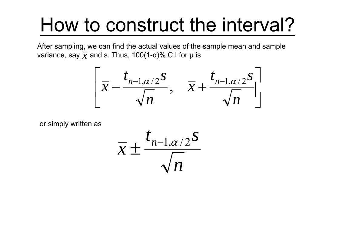
How to construct the interval?x
After sampling, we can find the actual values of the sample mean and sample variance, say and s. Thus, 100(1-α)% C.I for μ is
⎥⎦
⎤⎢⎣
⎡+− −− st
xst
x nn 2/,12/,1 , αα⎥⎦
⎢⎣ nn
,
or simply written as
stx n 2/,1α−±
nx ,±

How to use the table of t distribution

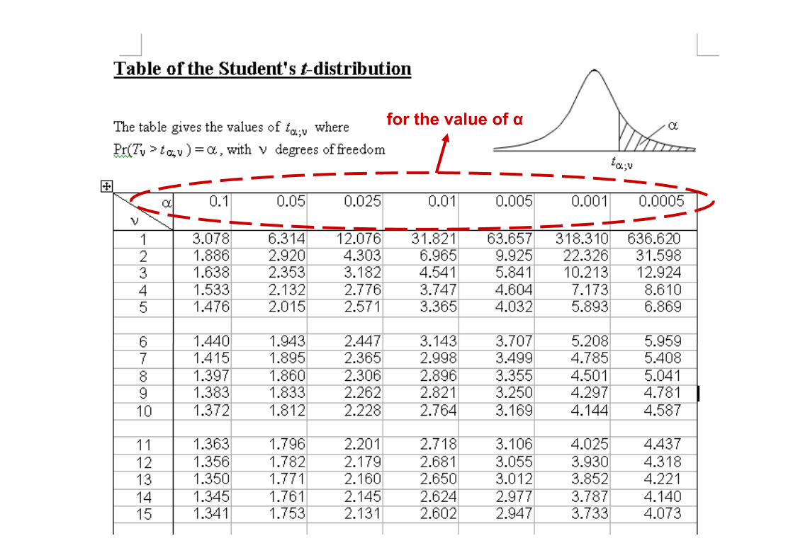
for the value of α

For the value of the degree of freedom

2.353 = ?

2.353 = ?t 3, 0.05
Degree of freedom first α
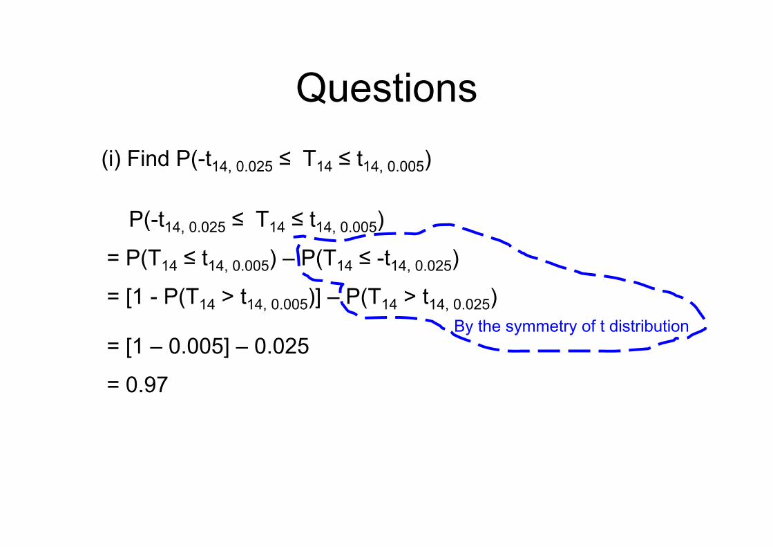
QuestionsQuestions(i) Find P(-t14, 0.025 ≤ T14 ≤ t14, 0.005)
P( t T t )P(-t14, 0.025 ≤ T14 ≤ t14, 0.005)
= P(T14 ≤ t14, 0.005) – P(T14 ≤ -t14, 0.025)
= [1 - P(T14 > t14, 0.005)] – P(T14 > t14, 0.025)By the symmetry of t distribution
= [1 – 0.005] – 0.025
= 0.97

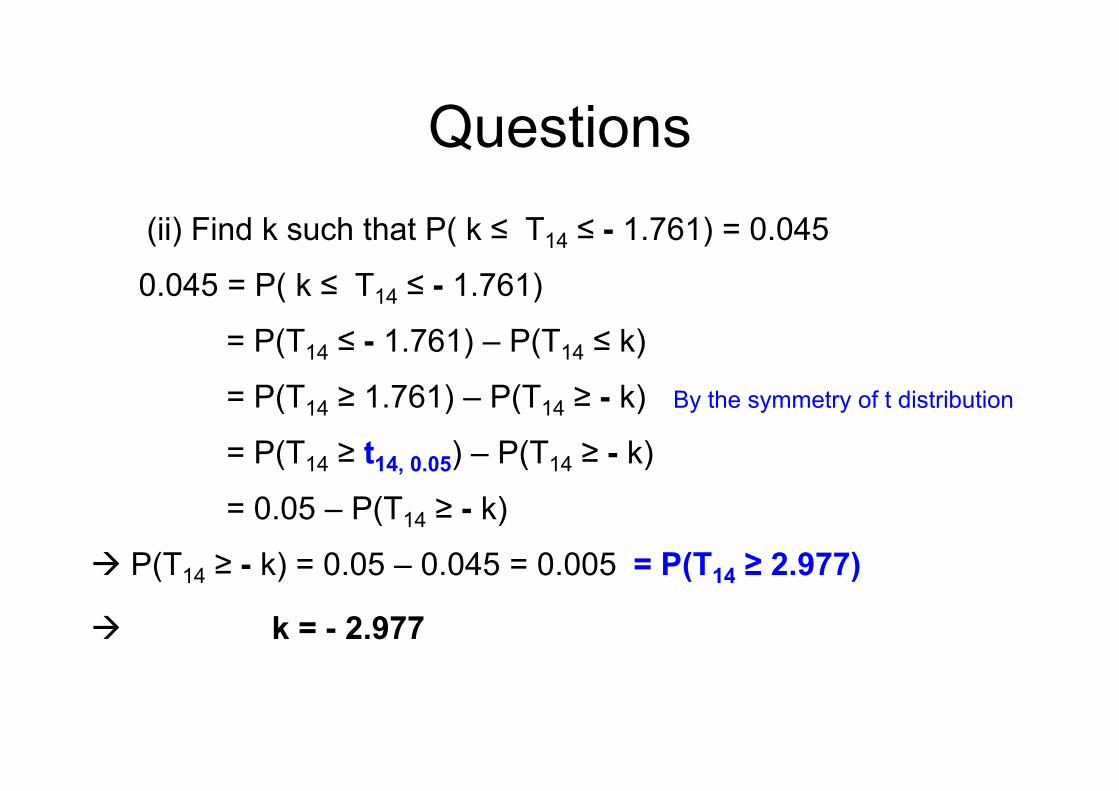
QuestionsQuestions(ii) Find k such that P( k ≤ T14 ≤ - 1.761) = 0.045
0.045 = P( k ≤ T14 ≤ - 1.761)
= P(T14 ≤ - 1.761) – P(T14 ≤ k)
= P(T ≥ 1 761) P(T ≥ k) By the symmetry of t distribution= P(T14 ≥ 1.761) – P(T14 ≥ - k) By the symmetry of t distribution


QuestionsQuestions(ii) Find k such that P( k ≤ T14 ≤ - 1.761) = 0.045
0.045 = P( k ≤ T14 ≤ - 1.761)
= P(T14 ≤ - 1.761) – P(T14 ≤ k)
= P(T ≥ 1 761) P(T ≥ k) By the symmetry of t distribution= P(T14 ≥ 1.761) – P(T14 ≥ - k) By the symmetry of t distribution
= P(T14 ≥ t14, 0.05) – P(T14 ≥ - k)
= 0.05 – P(T14 ≥ - k)
P(T14 ≥ - k) = 0.05 – 0.045 = 0.005 ( 14 ) 0 05 0 0 5 0 005

QuestionsQuestions(ii) Find k such that P( k ≤ T14 ≤ - 1.761) = 0.045
0.045 = P( k ≤ T14 ≤ - 1.761)
= P(T14 ≤ - 1.761) – P(T14 ≤ k)
= P(T ≥ 1 761) P(T ≥ k) By the symmetry of t distribution= P(T14 ≥ 1.761) – P(T14 ≥ - k) By the symmetry of t distribution
= P(T14 ≥ t14, 0.05) – P(T14 ≥ - k)
= 0.05 – P(T14 ≥ - k)
P(T14 ≥ - k) = 0.05 – 0.045 = 0.005 = P(T14 ≥ 2.977)( 14 ) 0 05 0 0 5 0 005 ( 14 9 )
k = - 2.977

QuestionsQuestionsFrequencies in hertz (Hz) of 12 elephant calls:Frequencies, in hertz (Hz), of 12 elephant calls:
14, 16, 17, 17, 24, 20, 32, 18, 29, 31, 15, 35
Assume that the population of possible elephant call frequencies is a normal distribution, Now a scientist is interested in the average of the frequencies, say µ. Find a 95% confidence interval for µ.
Population variance is UNKNOWN
So use t distribution to construct the C I for µSo, use t distribution to construct the C.I. for µ.
,33.22=x s2 = 56.424, n = 12, α = 0.05
Finally, the 95% C.I. for µ is [17.557, 27.103]
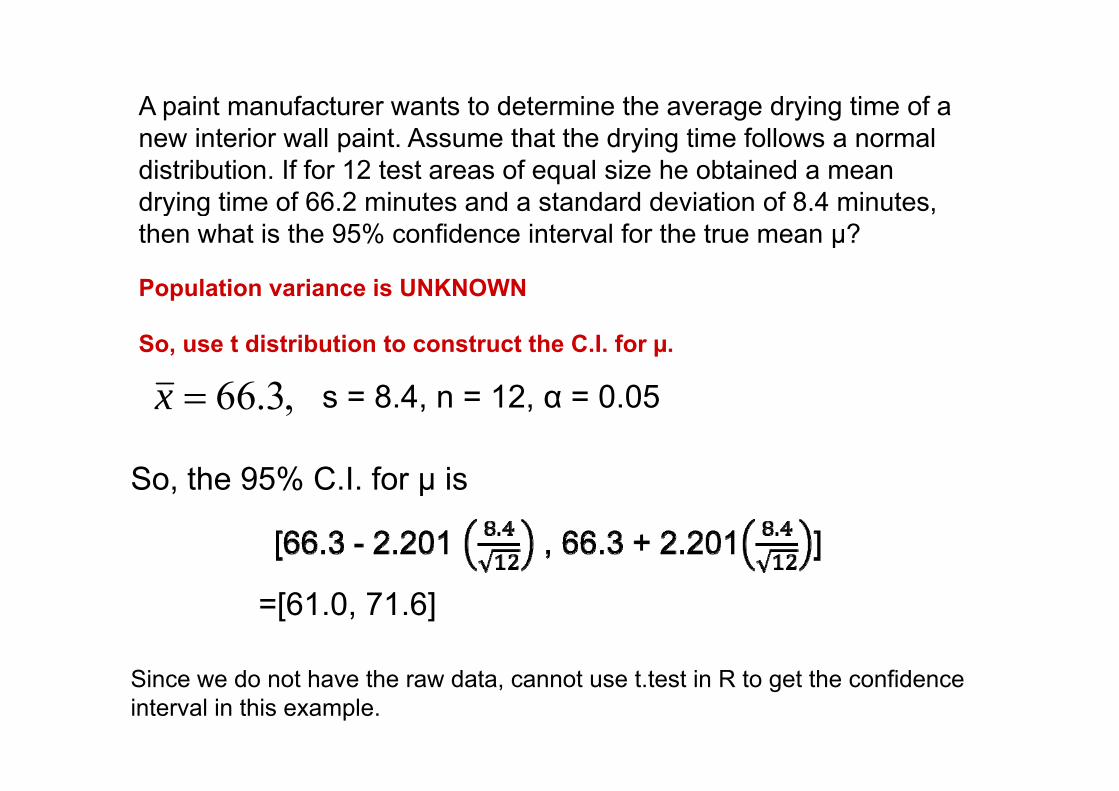
A paint manufacturer wants to determine the average drying time of a new interior wall paint. Assume that the drying time follows a normal distribution. If for 12 test areas of equal size he obtained a mean drying time of 66.2 minutes and a standard deviation of 8.4 minutes, y gthen what is the 95% confidence interval for the true mean μ?
Population variance is UNKNOWN
So, use t distribution to construct the C.I. for µ.
366=x s = 8 4 n = 12 α = 0 05,3.66=x s = 8.4, n = 12, α = 0.05
So the 95% C I for µ isSo, the 95% C.I. for µ is
=[61.0, 71.6]
Since we do not have the raw data, cannot use t.test in R to get the confidence interval in this example.

Remark:When n > 30, the difference of a t distribution with n -1 degrees of freedom and the standard normal distribution gis small. So, we have
zt ≈ .2/2/,1 αα ztn ≈−
Th fTherefore, we can use
⎥⎤
⎢⎡ +
szxszx 2/2/ αα⎥⎦⎢⎣
+−n
xn
x ,
to approximate the 100(1-α)% C.I for μ with unknown variance, as n > 30.
Two samples
Confidence Interval for µX - µY withConfidence Interval for µX µY with NORMAL populations
(k i )(known variances)

Confidence interval for µ µConfidence interval for µX - µYCase I: Normal distributions with unknown means and KNOWN variances:
Consider two independent random samples,
)( 2NXX σμ ),(~,,1 XXn NXX σμK
)( 2NYY σμand
),(~,,1 YYm NYY σμK
Want to construct a C I for the mean difference µX - µYWant to construct a C.I. for the mean difference µX µY.
First, choose a point estimator of the mean difference.
YX −use to estimate µX - µY.YX

How to construct the interval?Second, find the sampling distribution of . Indeed, we have a result that YX −
⎟⎞
⎜⎛ 22 σσ
⎟⎟⎠
⎞⎜⎜⎝
⎛+−−
mnNYX YX
YX ,~)(σσ
μμ
Or equivalently,
( )1,0~)()( NYX YX μμ −−− ( )1,022
N
mnYX σσ
+
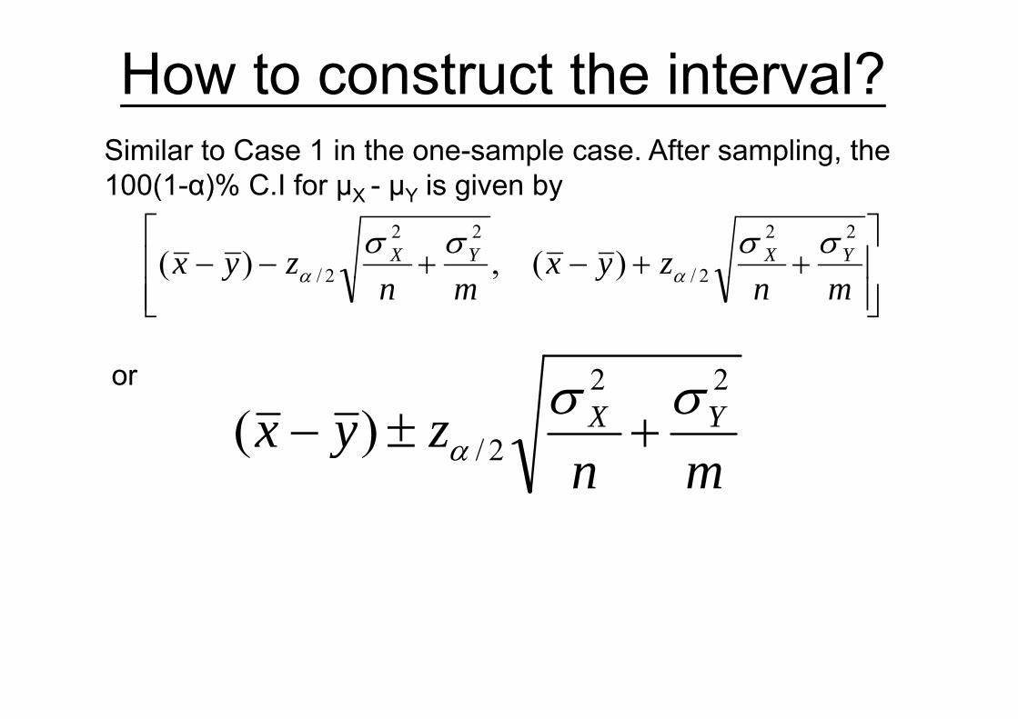
How to construct the interval?Similar to Case 1 in the one-sample case. After sampling, the 100(1-α)% C.I for μX - μY is given by
⎥⎥⎤
⎢⎢⎡
++−+−− zyxzyx YXYX22
2/
22
2/ )(,)( σσσσαα
( ) μX μY g y
⎥⎥⎦⎢
⎢⎣ mn
ymn
y 2/2/ )(,)( αα
zyx YX22
2/)( σσ+±−
or
mnzyx 2/)( α +±

Confidence interval for µ µConfidence interval for µX - µYCase I: Normal distributions with unknown means and KNOWN variances:
In particular, if two variances are EQUAL, say σX2 = σY
2 = σ2,
then the 100(1-α)% C.I for μX - μY becomes
⎥⎤
⎢⎡
++−+−− zyxzyx 11)(,11)( 2/2/ σσ ⎥⎦
⎢⎣
+++mn
zyxmn
zyx )(,)( 2/2/ σσ αα

ExampleExampleTwo kinds of thread are being compared for strength. Fifty pieces of each type of thread are tested under similar conditions. Brand A had an average tensile strength of 78.3 kil ith l ti t d d d i ti f 5 6 kilkilograms with a population standard deviation of 5.6 kilograms, while brand B had an average tensile strength of 87.2 kilograms with a population standard deviation of 6 3 kilogramskilograms with a population standard deviation of 6.3 kilograms. Construct a 95% confidence interval for the difference of the population means µA - µB.

Example n = m = 50ExampleTwo kinds of thread are being compared for strength. Fifty
n = m = 50
pieces of each type of thread are tested under similar conditions. Brand A had an average tensile strength of 78.3 kil ith l ti t d d d i ti f 5 6 kilkilograms with a population standard deviation of 5.6 kilograms, while brand B had an average tensile strength of 87.2 kilograms with a population standard deviation of 6 3 kilogramskilograms with a population standard deviation of 6.3 kilograms. Construct a 95% confidence interval for the difference of the population means µA - µB. α = 0.05
Two samples Known variances
378 287 5 6 6 3
α 0.05
3.78=x 2.87=y σX = 5.6 σY = 6.3

ExampleExampleTwo kinds of thread are being compared for strength. Fifty pieces of each type of thread are tested under similar conditions. Brand A had an average tensile strength of 78.3 kil ith l ti t d d d i ti f 5 6 kilkilograms with a population standard deviation of 5.6 kilograms, while brand B had an average tensile strength of 87.2 kilograms with a population standard deviation of 6 3 kilogramskilograms with a population standard deviation of 6.3 kilograms. Construct a 95% confidence interval for the difference of the population means µA - µB.
3.66.5)961()287378(22
+±−5050
)96.1()2.873.78( +±
= [-11.24, -6.56][ , ]
Two samples
Confidence Interval for µX - µY withConfidence Interval for µX µY with NORMAL populations( k i )(unknown variances)

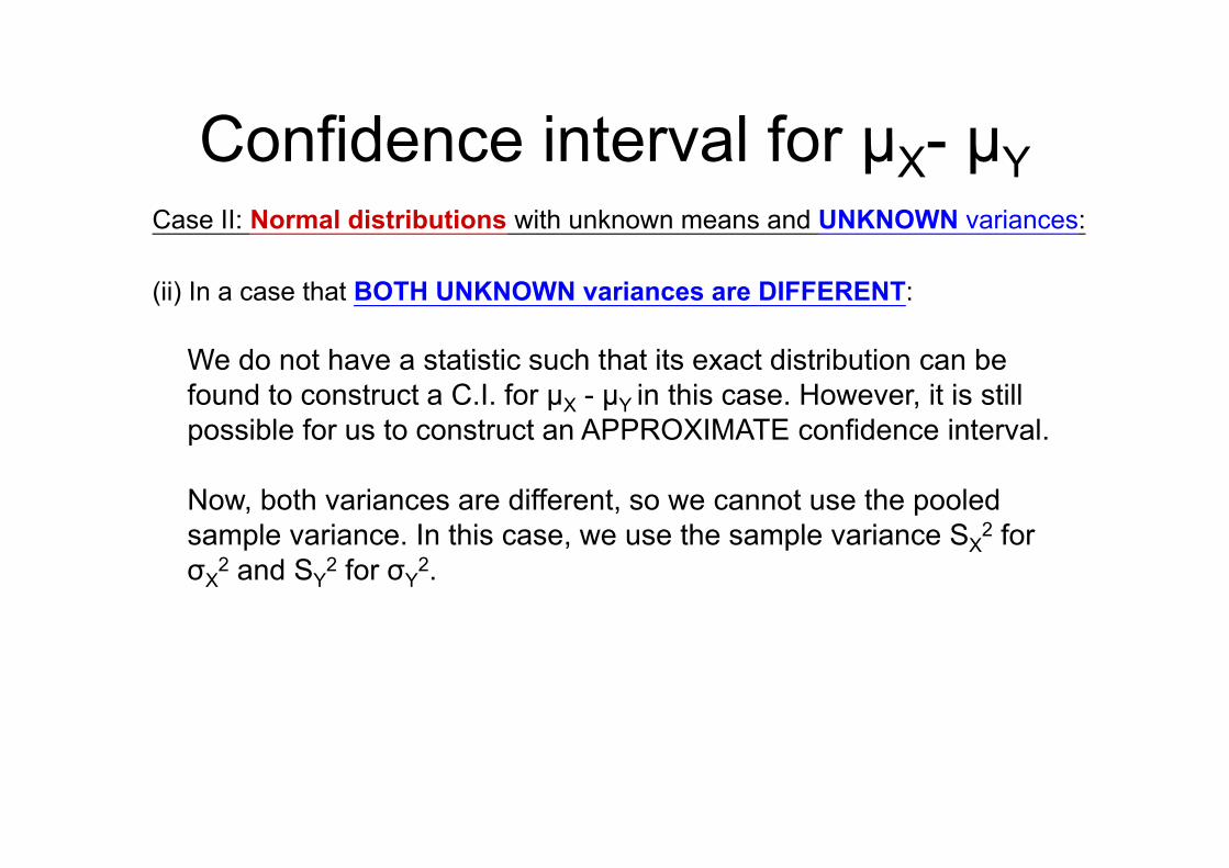
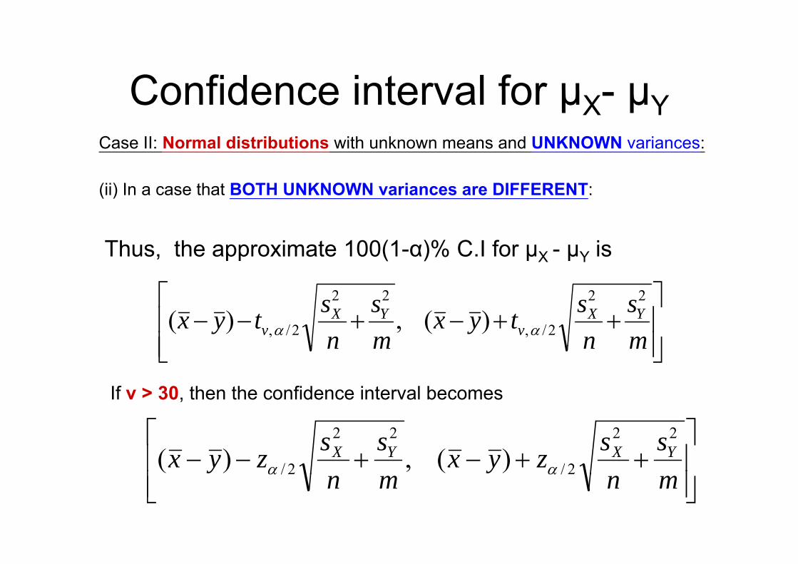
Confidence interval for µ µConfidence interval for µX - µYCase II: Normal distributions with unknown means and UNKNOWN variances:
Consider two independent random samples,
2 ),(~,, 21 XXn NXX σμK
)( 2and
),(~,, 21 YYm NYY σμK
(i) In a case that BOTH UNKNOWN variances are EQUAL:
(ii) In a case that BOTH UNKNOWN variances are DIFFERENT:
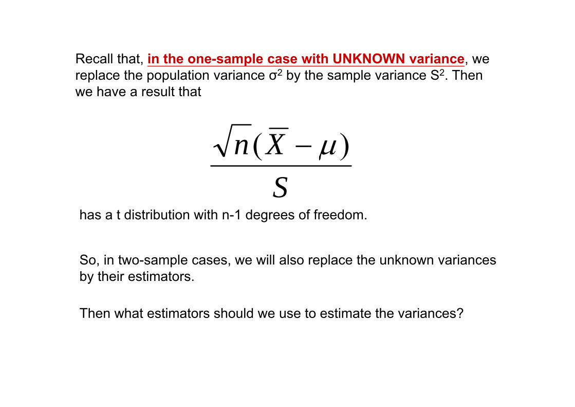
Recall that, in the one-sample case with UNKNOWN variance, we , p ,replace the population variance σ2 by the sample variance S2. Then we have a result that
Xn )( μ−S
)( μ
has a t distribution with n-1 degrees of freedom.
So, in two-sample cases, we will also replace the unknown variances by their estimators.
Then what estimators should we use to estimate the variances?

Confidence interval for µ µConfidence interval for µX - µYCase II: Normal distributions with unknown means and UNKNOWN variances:
(i) In a case that BOTH UNKNOWN variances are EQUAL:
Use a statistic
)()( 22
2−+−∑ ∑ YYXX
n m
ji
21 12
−+= = =
mnS i i
p
)1()1( 22 −+−=
SmSn YX
which is called a pooled estimator of σ2 or pooled sample variance
2−+mnwhich is called a pooled estimator of σ or pooled sample variance.
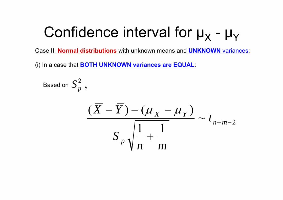
Confidence interval for µ µConfidence interval for µX - µYCase II: Normal distributions with unknown means and UNKNOWN variances:
(i) In a case that BOTH UNKNOWN variances are EQUAL:
Based on ,2pS
2~)()(−+
−−−mn
YX tYX μμ211 −+
+mn
p mnS
mn

So, after sampling, the 100(1-α)% C.I for μX - μY is given by
11)( ±mn
styx pmn)( 2/,2 +±− −+ α
If n+m-2 > 30, then the confidence interval can be approximated by
11)( ±mn
szyx p)( 2/ +±− α

ExampleExamplePage 18
Two tomato fertilizers are compared to see if one is better than the other.
Th i ht t f t i d d t d l fThe weight measurements of two independent random samples of tomatoes grown using each of the two fertilizers (in ounces) are as follows:
Fertilizer A (X): 12, 11, 7, 13, 8, 9, 10, 13
Fertilizer B (Y): 13 11 10 6 7 4 10Fertilizer B (Y): 13, 11, 10, 6, 7, 4, 10
Assume that two populations are normal and their population variances areAssume that two populations are normal and their population variances are equal. Consider a confidence level 1-α = 0.95.

Fertilizer A (X): 12, 11, 7, 13, 8, 9, 10, 13( )
Fertilizer B (Y): 13, 11, 10, 6, 7, 4, 10
A th t t l ti l d th i l ti i lAssume that two populations are normal and their population variances are equal. Consider a confidence level 1-α = 0.95.
Since n = 8 m = 7 37510=x ,714.8=y 12552 =Xs andSince n = 8, m = 7, ,375.10=x ,714.8y 125.5Xs,905.92 =Ys
and
)1()1( 22 + smsn 331.72)1()1(2 =
+−−+−
=mn
smsns YXp
Thus, the 95% C.I. for µX - µY is given by
11 )71
81(331.7)714.8375.10( 025.0,13 +±− t
= [-1.366, 4.688].
Confidence interval for µ µConfidence interval for µX- µYCase II: Normal distributions with unknown means and UNKNOWN variances:
(ii) In a case that BOTH UNKNOWN variances are DIFFERENT:
We do not have a statistic such that its exact distribution can be found to construct a C.I. for µX - µY in this case. However, it is still possible for us to construct an APPROXIMATE confidence intervalpossible for us to construct an APPROXIMATE confidence interval.
Now, both variances are different, so we cannot use the pooled sample variance In this case we use the sample variance S 2 forsample variance. In this case, we use the sample variance SX
2 for σX
2 and SY2 for σY
2.

That is, we consider
)()( YX YX −−− μμ .)()(22 SS YX
YX
+
μμ
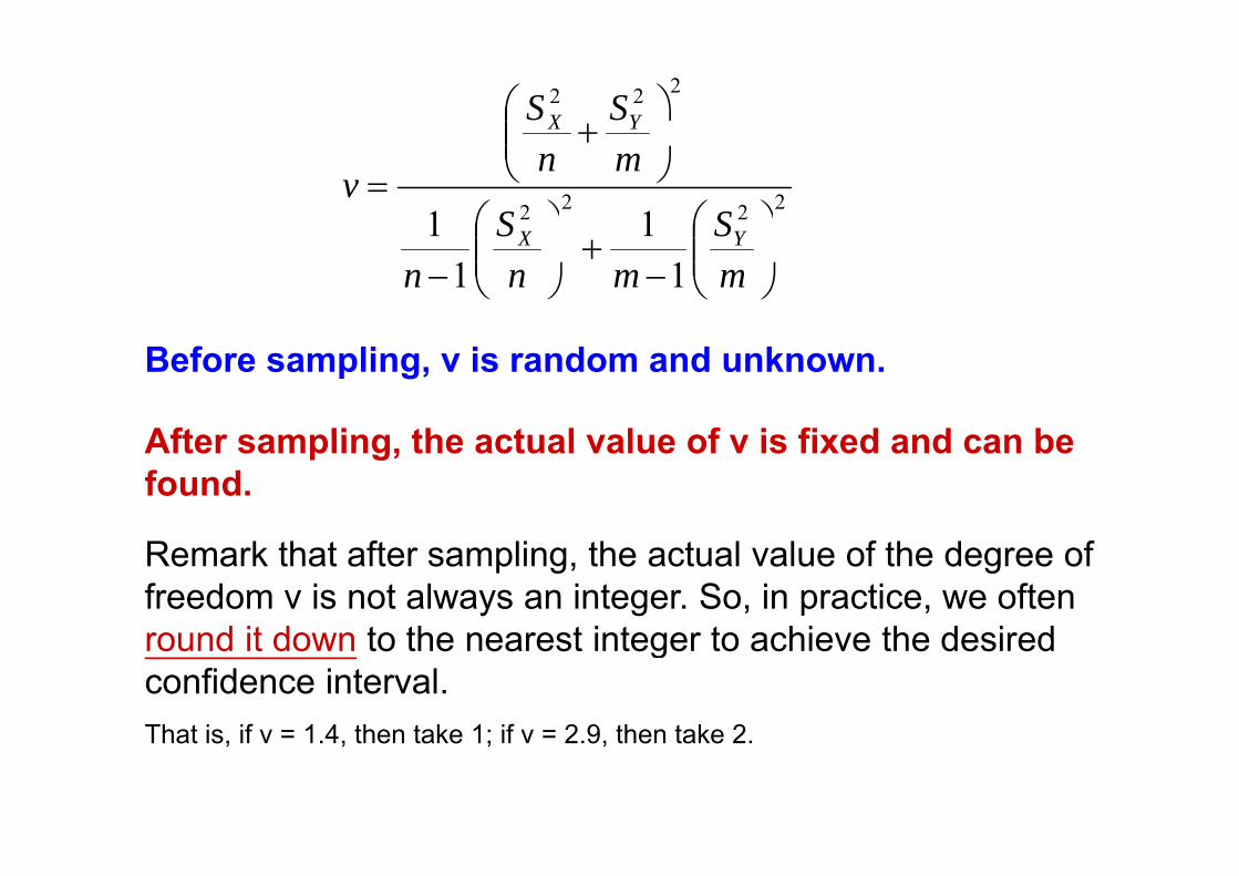
mnIt can be shown that the sampling distribution of the aboveIt can be shown that the sampling distribution of the above statistic is an approximate t distribution with v degrees of freedom, where 222 ⎞⎛ SS
22
22
⎟⎟⎠
⎞⎜⎜⎝
⎛+
=mS
nS
v
YX
2222
11
11
⎟⎟⎠
⎞⎜⎜⎝
⎛−
+⎟⎟⎠
⎞⎜⎜⎝
⎛− m
Smn
Sn
vYX
⎠⎝⎠⎝
222
⎟⎟⎞
⎜⎜⎛
+SS YX
2222 11⎟⎟⎞
⎜⎜⎛
⎟⎟⎞
⎜⎜⎛
⎟⎟⎠
⎜⎜⎝
+=
SS
mnv
YX
11 ⎟⎟⎠
⎜⎜⎝−
+⎟⎟⎠
⎜⎜⎝− mmnn
YX
Before sampling, v is random and unknown.
After sampling the actual value of v is fixed and can beAfter sampling, the actual value of v is fixed and can be found.
Remark that after sampling, the actual value of the degree of freedom v is not always an integer. So, in practice, we often round it down to the nearest integer to achieve the desiredround it down to the nearest integer to achieve the desired confidence interval.That is if v = 1 4 then take 1; if v = 2 9 then take 2That is, if v = 1.4, then take 1; if v = 2.9, then take 2.
Confidence interval for µ µConfidence interval for µX- µYCase II: Normal distributions with unknown means and UNKNOWN variances:
(ii) In a case that BOTH UNKNOWN variances are DIFFERENT:
⎤⎡
Thus, the approximate 100(1-α)% C.I for μX - μY is
⎥⎥⎦
⎤
⎢⎢⎣
⎡++−+−−
ms
nstyx
ms
nstyx YX
vYX
v
22
2/,
22
2/, )(,)( αα⎥⎦⎢⎣ mnmn
If v > 30, then the confidence interval becomes
⎥⎥⎤
⎢⎢⎡
++−+−−sszyxsszyx YXYX22
2/
22
2/ )(,)( αα⎥⎦⎢⎣ mnmn 2/2/ αα

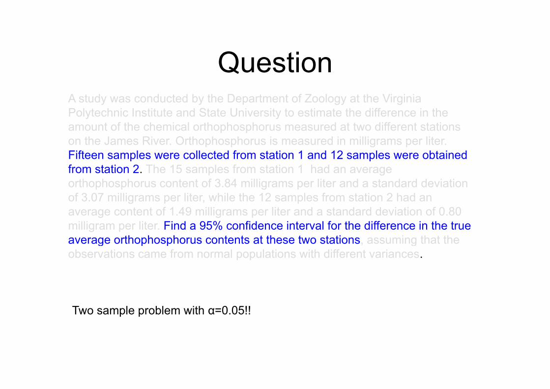
QuestionQuestionA study was conducted by the Department of Zoology at the Virginia Polytechnic Institute and State University to estimate the difference in the amount of the chemical orthophosphorus measured at two different stations on the James River. Orthophosphorus is measured in milligrams per liter.
f fFifteen samples were collected from station 1 and 12 samples were obtained from station 2. The 15 samples from station 1 had an average orthophosphorus content of 3.84 milligrams per liter and a standard deviation
f 3 07 illi lit hil th 12 l f t ti 2 h dof 3.07 milligrams per liter, while the 12 samples from station 2 had an average content of 1.49 milligrams per liter and a standard deviation of 0.80 milligram per liter. Find a 95% confidence interval for the difference in the true average orthophosphorus contents at these two stations assuming that theaverage orthophosphorus contents at these two stations, assuming that the observations came from normal populations with different variances.
Two sample problem with α=0.05!!

QuestionQuestionA study was conducted by the Department of Zoology at the Virginia Polytechnic Institute and State University to estimate the difference in the amount of the chemical orthophosphorus measured at two different stations on the James River. Orthophosphorus is measured in milligrams per liter.
f fFifteen samples were collected from station 1 and 12 samples were obtained from station 2. The 15 samples from station 1 had an average orthophosphorus content of 3.84 milligrams per liter and a standard deviation
f 3 07 illi lit hil th 12 l f t ti 2 h dof 3.07 milligrams per liter, while the 12 samples from station 2 had an average content of 1.49 milligrams per liter and a standard deviation of 0.80 milligram per liter. Find a 95% confidence interval for the difference in the true average orthophosphorus contents at these two stations assuming that theaverage orthophosphorus contents at these two stations, assuming that the observations came from normal populations with different variances.
Normal!! Different VariancesTwo sample problem with α=0.05!!

QuestionQuestionA study was conducted by the Department of Zoology at the Virginia Polytechnic Institute and State University to estimate the difference in the amount of the chemical orthophosphorus measured at two different stations on the James River. Orthophosphorus is measured in milligrams per liter.
f fFifteen samples were collected from station 1 and 12 samples were obtained from station 2. The 15 samples from station 1 had an average orthophosphorus content of 3.84 milligrams per liter and a standard deviation
f 3 07 illi lit hil th 12 l f t ti 2 h dof 3.07 milligrams per liter, while the 12 samples from station 2 had an average content of 1.49 milligrams per liter and a standard deviation of 0.80 milligram per liter. Find a 95% confidence interval for the difference in the true average orthophosphorus contents at these two stations assuming that theaverage orthophosphorus contents at these two stations, assuming that the observations came from normal populations with different variances.
Normal!! Different VariancesTwo sample problem with α=0.05!!15073843 nsx 1280491 msyd15,07.3,84.3 === nsx X 12,8.0,49.1 === msy Yand

QuestionQuestionNormal!! Different VariancesTwo sample problem with α=0.05!!
103843 128049115,07.3,84.3 === nsx X 12,8.0,49.1 === msy Yand
Consider µ1 - µ2, where µi is the true average orthophosphorus contents at station i, i = 1 and 2.
Since the population variances are assumed to be unequal, we can only find an i 9 % C I b d h di ib i i h d f f dapproximate 95% C.I. based on the t distribution with v degrees of freedom,
where
( )12/80015/073 222 +( )]11/)12/80.0[(]14/)15/07.3[(
12/80.015/07.32222 +
+=v
])[(])[(163.16 ≈=

QuestionQuestionNormal!! Different VariancesTwo sample problem with α=0.05!!
So, for α = 0.05, we have
1202=≈ tt 120.2025.0,162/, =≈ ttv α
Thus, the 95% C.I. for µ1 - µ2 is
sst YX22
)( +±
, µ1 µ2
mntyx YX
025.0,16)( +±−
].10.4,60.0[=1280.0
1507.3)120.2()49.184.3(
22
+±−=1215
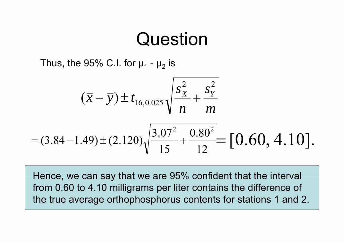
QuestionQuestionThus, the 95% C.I. for µ1 - µ2 is
sst YX22
)( ±
us, t e 95% C o µ1 µ2 s
mntyx YX
025.0,16)( +±−
].10.4,60.0[=1280.0
1507.3)120.2()49.184.3(
22
+±−=1215
Hence we can say that we are 95% confident that the intervalHence, we can say that we are 95% confident that the interval from 0.60 to 4.10 milligrams per liter contains the difference of the true average orthophosphorus contents for stations 1 and 2.g p p
One- (or Two-) sample(s)
Confidence Interval for µX (or µX - µY)Confidence Interval for µX (or µX µY) with NON-NORMAL population(s)
Approximate C I in One sample caseApproximate C.I. in One-sample case
Note that so far all results are based on the normalNote that, so far, all results are based on the normal population(s). Then a natural question is:
how to construct a C.I. with NON-Normal distribution.
U f t t l i l it i t t fi d t ti tiUnfortunately, in general, it is not easy to find a statistic such that its exact distribution is easily found in this case.
However, if the sample size is large enough, then we can use a normal approximation to approximate the pp ppdistribution of the statistic used to construct the C.I.

Central Limit Theorem (CLT)Central Limit Theorem (CLT)
XIf is the sample mean of a random sample X1,…, Xnof size n from any distribution with a finite mean µ
d fi it iti i 2 th th di t ib ti
X
μnXn
∑and a finite positive variance σ2, then the distribution of
μμ
nXX i
i∑=
−=
− 1
σσ nn/is the standard normal distribution N(0,1) in the limit as ngoes to infinity.

Approximate C I for µApproximate C.I. for µCase I: Any distribution with unknown mean and KNOWN variance:
Consider a random sample of size n, {X1, X2, …, Xn}, from a distributionwith unknown mean µ and KNOWN variance σ2. That is,
xAfter sampling, we can find an actual value of the sample mean, say . Thus, the APPROXIMATE 100(1-α)% C.I for μ is
⎥⎤
⎢⎡ +
zxzx σσ αα 2/2/
APPROXIMATE 100(1 α)% C.I for μ is
⎥⎦⎢⎣+−
nx
nx αα 2/2/ ,

Case II: Any distribution with unknown mean and UNKNOWN variance:
After sampling, we can find the actual values of the sample mean and sample i d Th th APPROXIMATE 100(1 )% C I f i
⎤⎡ stst 2/12/1 αα
xvariance, say and s. Thus, the APPROXIMATE 100(1-α)% C.I for μ is
⎥⎦
⎤⎢⎣
⎡+− −−
nst
xn
stx nn 2/,12/,1 , αα
If n is large enough, then the approximate 100(1-α)% C.I for μ becomes
⎥⎦
⎤⎢⎣
⎡ +−szxszx 2/2/ , αα⎥⎦⎢⎣ nn
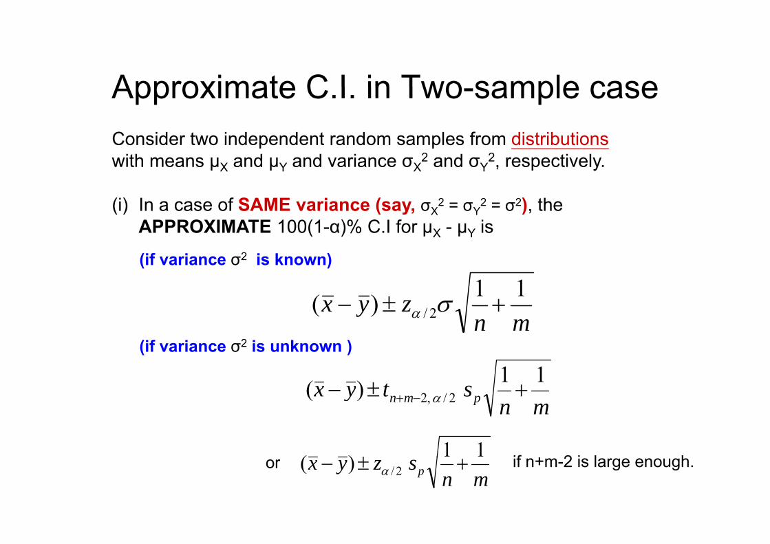
Approximate C I in Two sample caseApproximate C.I. in Two-sample caseConsider two independent random samples from distributionsp pwith means µX and µY and variance σX
2 and σY2, respectively.
(i) In a case of SAME variance (say, σX2 = σY
2 = σ2), the(i) In a case of SAME variance (say, σX σY σ ), the APPROXIMATE 100(1-α)% C.I for µX - µY is
(if variance σ2 is known)
mnzyx 11)( 2/ +±− σα
(if variance σ2 is unknown )
styx 11)( 2/2 +±− + mnstyx pmn)( 2/,2 +± −+ α
11)( ± if 2 i l hmn
szyx p)( 2/ +±− αor if n+m-2 is large enough.

Approximate C I in Two sample caseApproximate C.I. in Two-sample caseConsider two independent random samples from distributionsp pwith means µX and µY and variance σX
2 and σY2, respectively.
(i) In a case of Different variances, the APPROXIMATE(i) In a case of Different variances, the APPROXIMATE100(1-α)% C.I for µX - µY is
(if variances are known )
mnzyx YX
22
2/)( σσα +±−
(if variances are unknown )
sstyx YX22
2/)( +±−mn
tyx v 2/,)( +± α
ss YX22
)( if i l h ORms
nszyx YX
2/)( +±− αor if v is large enough OR n and m are large enough.

Confidence Interval for σ2
with NORMAL population
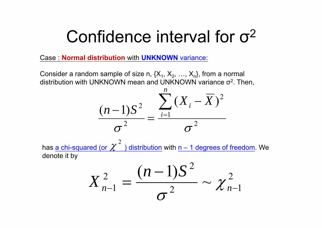
Confidence interval for σ2Confidence interval for σ2
Case : Normal distribution with UNKNOWN variance:
Consider a random sample of size n, {X1, X2, …, Xn}, from a normal distribution with UNKNOWN mean and UNKNOWN variance σ2. Then,
1
22 )(
)1( ∑ −−
n
ii XX
Sn2
12
)(σσ
== i
2has a chi-squared (or ) distribution with n – 1 degrees of freedom. We denote it by
2χ
2)1( S 212
221 ~)1(
−−−
= nnSnX χ2σ

Chi-squared distribution with k degrees of freedom
Not symmetric !!Not symmetric !!
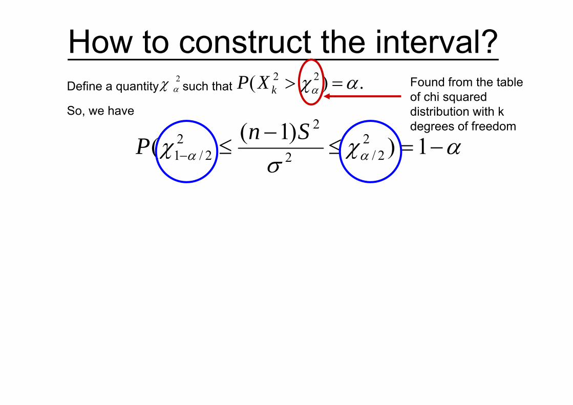
How to construct the interval?
So we have
2αχ .)( 22 αχα =>kXPDefine a quantity such that Found from the table
of chi squared distribution with k
αχχ αα −=≤−
≤− 1))1(( 22/2
22
2/1SnP
So, we have distribution with k degrees of freedom
χσ
χ αα )( 2/22/1

Density function of the chi-squared random variable21−nX 1n
with n-1 degrees of freedom.
2/α
2/α/α
1 α−1
22/αχ
22/1 αχ −

How to construct the interval?
So we have
2αχ .)( 22 αχα =>kXPDefine a quantity such that Found from the table
of chi squared distribution with k
αχχ αα −=≤−
≤− 1))1(( 22/2
22
2/1SnP
So, we have distribution with k degrees of freedom
χσ
χ αα )( 2/22/1
−− )1()1( 22
2 SnSn αχ
σχ αα
−=≤≤−
1))1()1(( 22/1
222/
SnSnP
22 ⎤⎡
After sampling, we can find an actual value of the sample variance, say s2. Thus, 100(1-α)% C.I for σ2 is
.)1(,)1(2
2
2
2
⎥⎦
⎤⎢⎣
⎡ −− snsn2
2/122/
⎥⎦
⎢⎣ −αα χχ
How to use the table of chi-squared distributiondistribution
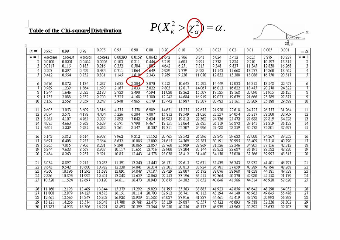
.)( 22 αχα =>kXP

for the value of α
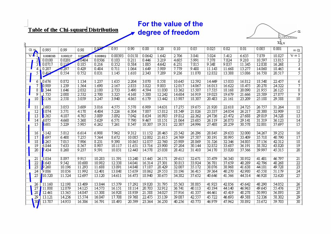
For the value of the degree of freedom

20.483 = ?

20.483 = ?2025.0χ
With 10 degrees of freedom

QuestionsQuestionsFor a chi-squared distribution with v degrees of freedom,
a) If v = 5, then
=2005.0χ

16.750 = 2005.0χ
With 5 degrees of freedom

QuestionsQuestionsFor a chi-squared distribution with v degrees of freedom,
a) If v = 5, then
750.162005.0 =χ
b) If v = 19, then
144.30205.0 =χ
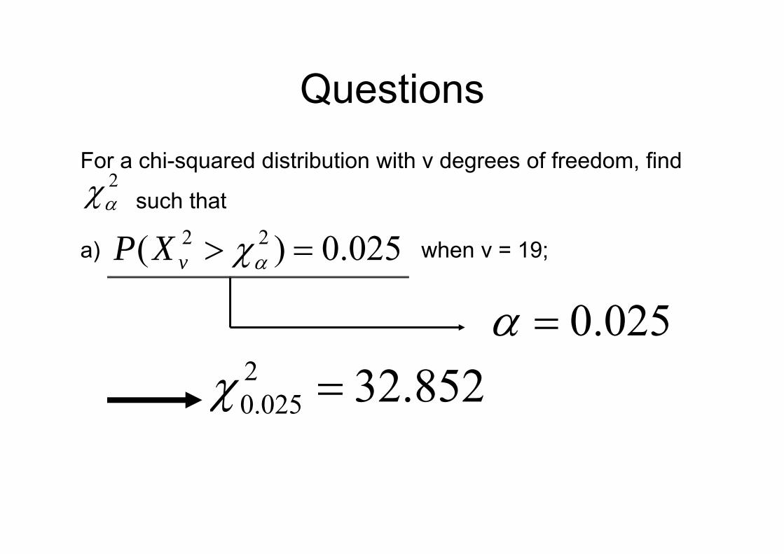
QuestionsQuestionsFor a chi-squared distribution with v degrees of freedom, find
such that2αχ
025.0)( 22 => αχvXPa) when v = 19;
025.0=α852.322
0250 =χ 025.0χ

QuestionsQuestionsFor a chi-squared distribution with v degrees of freedom, find
such that2αχ
045.0)652.37( 22 =<< αχvXPb) when v = 25;
)652.37()( 225
2225 αχ <−<= XPXP
)()652.37( 2225
225 αχ>−>= XPXP
?= ?

)652.37( 225 >XP
37 652 =2χ37.652 = 05.0χ
With 25 degrees of freedom

QuestionsQuestionsFor a chi-squared distribution with v degrees of freedom, find
such that2αχ
045.0)652.37( 22 =<< αχvXPb) when v = 25;
)652.37()( 225
2225 αχ <−<= XPXP
)()652.37( 2225
225 αχ>−>= XPXP
)(05.0 2225 αχ>−= XP
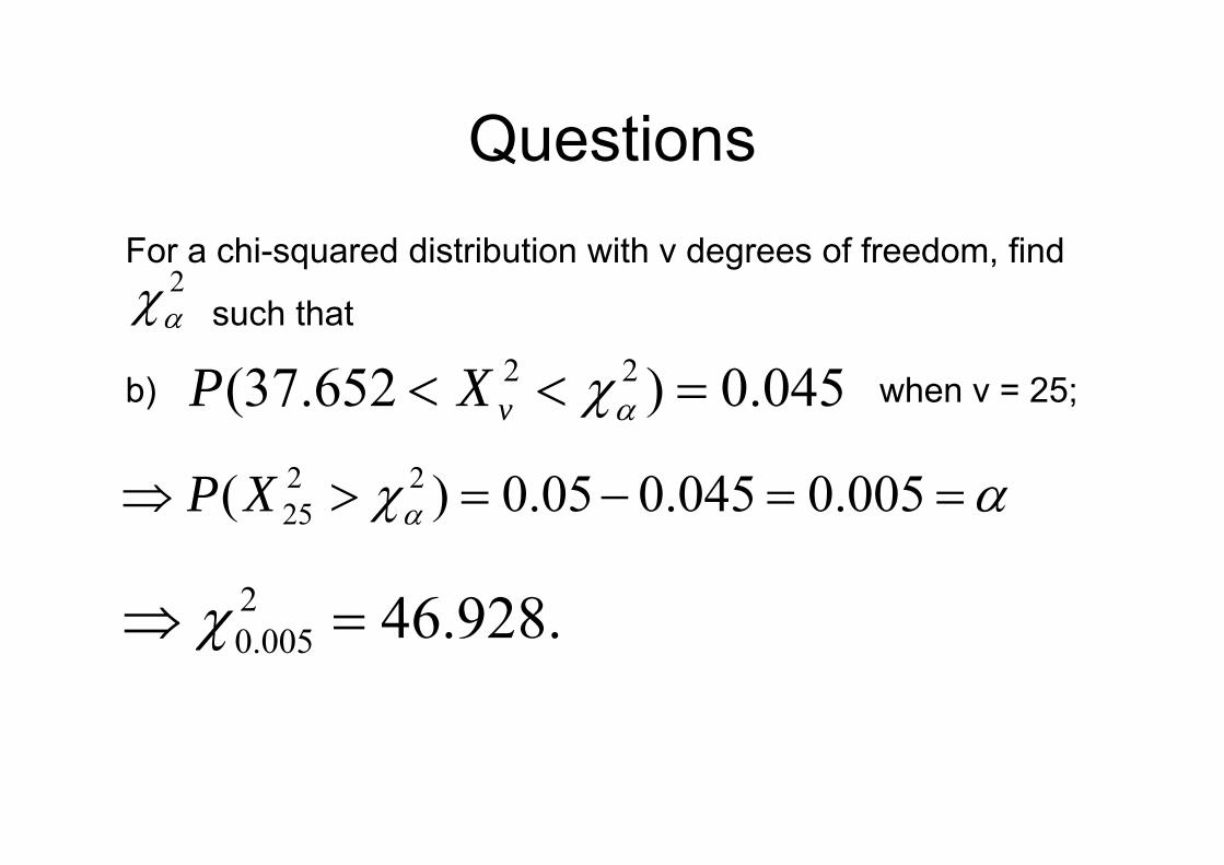
QuestionsQuestionsFor a chi-squared distribution with v degrees of freedom, find
such that2αχ
045.0)652.37( 22 =<< αχvXPb) when v = 25;
αχα ==−=>⇒ 005.0045.005.0)( 2225XP
928462 =⇒ χ .928.46005.0 =⇒ χ
QuestionsQuestionsFor a chi-squared distribution with v degrees of freedom, find
such that2αχ
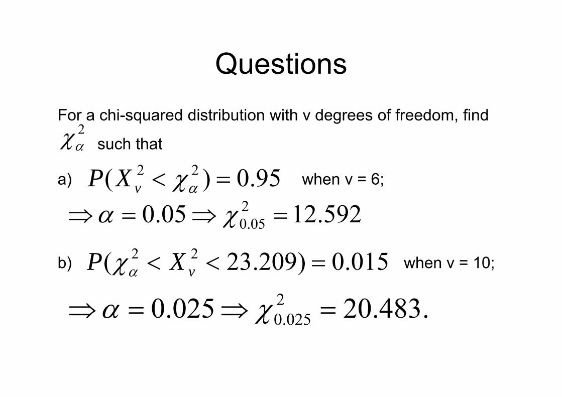
95.0)( 22 =< αχvXPa) when v = 6;
592.1205.0 205.0 =⇒=⇒ χα
015.0)209.23( 22 =<< vXP αχb) when v = 10;
.483.20025.0 2025.0 =⇒=⇒ χα

How about the confidence interval for σ, not σ2?
ασ −=−
≤≤− 1))1()1(( 2
22
2
2 SnSnPRecall that
A 100(1 )% fid i t l f b bt i d
χχ αα −
)( 22/1
22/
A 100(1 - α)% confidence interval for σ can be obtained by taking the square root of each endpoint of the interval for σ2 That isfor σ . That is,
)1()1(⎥⎤
⎢⎡ −− snsn
.)1(
,)1(
22/1
22/ ⎥
⎥⎦⎢
⎢⎣ αα χχ
snsn
2/12/ ⎥⎦⎢⎣ −αα χχ

ExampleExampleThe following are the weights, in decagrams, of 10 e o o g a e t e e g ts, decag a s, o 0packages of grass seed distributed by a certain company:
46 4 46 1 45 8 47 0 46 1 45 9 45 8 46 9 45 2 d 46 046.4, 46.1, 45.8, 47.0, 46.1, 45.9, 45.8, 46.9, 45.2 and 46.0.
Find a 95% C I for the variance of all such packages ofFind a 95% C.I. for the variance of all such packages of grass seed distributed by this company, assuming that a normal population is used.p p

Example n = 10ExampleThe following are the weights, in decagrams, of 10
n = 10
e o o g a e t e e g ts, decag a s, o 0packages of grass seed distributed by a certain company:
46 4 46 1 45 8 47 0 46 1 45 9 45 8 46 9 45 2 d 46 046.4, 46.1, 45.8, 47.0, 46.1, 45.9, 45.8, 46.9, 45.2 and 46.0.
Find a 95% C I for the variance of all such packages ofFind a 95% C.I. for the variance of all such packages of grass seed distributed by this company, assuming that a normal population is used.p p
05.0=α023.192025.0
22/ == χχα
700.22975.0
22/1 ==− χχ α

Example n = 10ExampleThe following are the weights, in decagrams, of 10
n = 10
e o o g a e t e e g ts, decag a s, o 0packages of grass seed distributed by a certain company:
46 4 46 1 45 8 47 0 46 1 45 9 45 8 46 9 45 2 d 46 046.4, 46.1, 45.8, 47.0, 46.1, 45.9, 45.8, 46.9, 45.2 and 46.0.
∑n
22 1 ∑=
=−−
=i
i xxn
s1
22 286.0)(11
Thus, the 95% C.I. for the variance is
)2860(9)2860(9 ].953.0,135.0[]7002
)286.0(9,02319)286.0(9[ =
700.2023.19

Sample size determinationSample size determinationBefore we end the topic of estimation let’s consider theBefore we end the topic of estimation, let s consider the problem of how to determine the sample size.
Often, we wish to know how large a sample is necessaryto ensure that the error in estimating an unknown gparameter, say µ, will be less than a specified amount e.
Consider a 100(1-α)% C.I. for µ with known variance. The (marginal) error is σ
nz σα 2/

Th l i f th l i i th tiThus, solving for the sample size n in the equation
σ en
z =σ
α 2/ nimplies that the required sample size isp q p
22/ ⎟
⎞⎜⎛ z σ .2/ ⎟
⎠⎞
⎜⎝⎛=
ezn σα
QuestionQuestion
A marketing research firm wants to conduct a survey to estimate the average amount spent on entertainment byestimate the average amount spent on entertainment by each person visiting a popular resort. The people who plan the survey would like to have an estimate close to the true value such that we will have 95% confidence that the difference between them is within $120. If the population standard deviation is $400 then how largepopulation standard deviation is $400, then how large should the sample be?

QuestionQuestion96.105.0 02502/ ==⇒= zzαα
A marketing research firm wants to conduct a survey to estimate the average amount spent on entertainment by
025.02/α
estimate the average amount spent on entertainment by each person visiting a popular resort. The people who plan the survey would like to have an estimate close tothe true value such that we will have 95% confidence that the difference between them is within $120. If the population standard deviation is $400 then how largepopulation standard deviation is $400, then how large should the sample be?
e120|| ≤−⇒ xμ 120±∈⇒ xμ
e
400400=σ
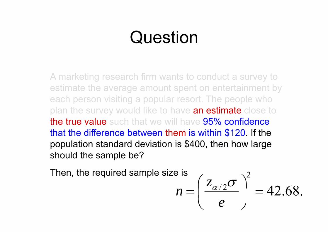
QuestionQuestion
A marketing research firm wants to conduct a survey to estimate the average amount spent on entertainment byestimate the average amount spent on entertainment by each person visiting a popular resort. The people who plan the survey would like to have an estimate close tothe true value such that we will have 95% confidence that the difference between them is within $120. If the population standard deviation is $400 then how largepopulation standard deviation is $400, then how large should the sample be?
Then, the required sample size is
.68.422
2/ =⎟⎞
⎜⎛=
zn σα .68.42⎟⎠
⎜⎝ e
n
Recommended