1
Centre for Investment Research Discussion Paper Series
Discussion Paper # 06-02*
Simulating Convertible Bond Arbitrage Portfolios
Mark Hutchinson University College Cork, Ireland
Liam Gallagher
Dublin City University, Ireland
Centre for Investment Research O'Rahilly Building, Room 3.02 University College Cork College Road Cork Ireland T +353 (0)21 490 2597/2765 F +353 (0)21 490 3346/3920 E [email protected] W www.ucc.ie/en/cir/ *These Discussion Papers often represent preliminary or incomplete work, circulated to encourage discussion and comments. Citation and use of such a paper should take account of its provisional character. A revised version may be available directly from the author(s).
2
Simulating Convertible Bond Arbitrage Portfolios
Mark Hutchinson* University College Cork, Ireland
Liam Gallagher** Dublin City University, Ireland
Abstract The recent growth in interest in convertible bond arbitrage (CBA) has predominately come from
the hedge fund industry. Past empirical evidence has shown that a CBA strategy generates
positive monthly abnormal risk adjusted returns. However, these studies have focused on hedge
fund returns which exhibit instant history bias, selection bias, survivorship bias and smoothing.
This paper replicates the core underlying CBA strategy to generate an equally weighted and
market capitalisation daily CBA return series free of these biases, for the period 1990 through to
2002. These daily series also capture important short-run price dynamics that previous studies
have ignored.
Keywords: Arbitrage, Convertible bonds, Hedge funds
We are grateful to SunGard Trading and Risk Systems for providing Monis Convertibles XL convertible bond analysis software and convertible bond terms and conditions. We thank an anonymous reviewer for helpful comments and suggestions.
*Address for Correspondence: Mark Hutchinson, Department of Accounting and Finance, University College Cork, College Road, Cork, Ireland. Telephone: +353 21 4902597, E-mail: [email protected] **Address for Correspondence: Liam Gallagher, DCU Business School, Dublin City University, Dublin 9, Ireland. Telephone: +353 1 7005399, E-mail: [email protected]
3
Simulating Convertible Bond Arbitrage Portfolios Abstract: The recent growth in interest in convertible bond arbitrage (CBA) has predominately come from the hedge fund industry. Past empirical evidence has shown that a CBA strategy generates positive monthly abnormal risk adjusted returns. However, these studies have focused on hedge fund returns which exhibit instant history bias, selection bias, survivorship bias and smoothing. This paper replicates the core underlying CBA strategy to generate an equally weighted and market capitalisation daily CBA return series free of these biases, for the period 1990 through to 2002. These daily series also capture important short-run price dynamics that previous studies have ignored.
1. Introduction
Convertible bond arbitrageurs derive returns from two areas, income and long volatility
exposure. Income comes from the coupon paid periodically by the issuer of the convertible bond
and from interest on the short stock position. To capture the long volatility exposure, the
arbitrageur initiates a dynamic hedging strategy. The hedge is rebalanced as the stock price
and/or convertible price move. Prior studies of convertible arbitrage hedge funds have
documented significant positive abnormal returns from the strategy. However, it is well known
that the hedge fund data contains several characteristics which upwardly bias these performance
estimates. In this paper we create a simulated convertible bond arbitrage portfolio free of these
biases, designed to capture income and volatility, and we also provide evidence of the historical
risk and performance of the strategy.
First issued in the United States in the nineteenth century, a simple convertible bond is
defined as a corporate bond, paying a fixed coupon, with security, maturing at a certain date with
an additional feature allowing it to be converted into a fixed number of the issuer’s common
stock. According to Calamos (2003) this convertible clause was first added to fixed income
investments to increase the attractiveness of investing in rail roads of what was then the emerging
economy of the United States. Convertible bonds have grown in complexity and are now issued
with features such as put options, call protection, ratchet clauses, step up coupons and floating
coupons. Perhaps due to this complexity relatively few individual or institutional investors
4
incorporate convertible into their portfolios. It has been estimated that hedge funds account for
seventy percent of the demand for new convertible issues and eighty percent of convertible
transactions (see Barkley, 2001; McGee, 2003).
While the overall market for convertible bonds has been growing to an estimated $351.9
billion by the end of December 2003 (BIS, 2004), the hedge fund industry has also been growing
at a phenomenal rate. Initially hedge fund investors were interested in large global/macro hedge
funds and the majority of the funds went into these strategies. Fung and Hsieh (2000a) estimate
that in 1997 twenty seven large hedge funds accounted for at least one third of the assets managed
by the industry. However, investors have been increasingly interested in lower volatility non-
directional arbitrage strategies. Data from Tremont Advisors and the Barclay Group indicate that
convertible arbitrage total market value grew from just $768m in 1994 to $64.9bn in 2004, an
astonishing growth rate of 50% on average per annum.
Academic literature on dynamic trading strategies has generally focused on modelling the
relationship between the returns of hedge funds which follow such strategies and the asset
markets and contingent claims on those assets in which hedge funds operate (see, for example,
Fung and Hsieh, 1997; Liang, 1999; Schneeweis and Spurgin, 1998; Capocci and Hübner, 2004;
Agarwal and Naik, 2004). The difficulty with these studies it that the use of hedge fund returns to
define the characteristics of a strategy introduces biases as discussed in Fung and Hsieh (2000b)
and Getmansky, Lo and Makarov (2004).
Hedge fund data contains four main biases, instant history bias, selection bias
survivorship bias and smoothing. An instant history bias occurs if hedge fund database vendors
back fill a hedge funds performance when they add it to a database. A selection bias occurs if the
hedge funds in an observable portfolio are not representative of that particular class of hedge
funds. Some funds may be classified as convertible arbitrage but may generally operate a long
only strategy. Survivorship bias occurs if funds drop out of a database due to poor performance.
The resulting database is therefore biased upwards as poor performing funds are excluded. Liang
5
(2000) examines the survivorship bias in hedge fund returns by comparing two large databases
(HFR and TASS) finding survivorship bias of 2% per year. Performance smoothing occurs if
hedge funds report only part of the gains in months when a fund has positive returns so as to
partially offset potential future losses and thereby reduce volatility and improve risk-adjusted
performance measures such as the Sharpe (1966) ratio and the Jensen (1968) alpha. Smoothing is
difficult to implement with liquid instruments, but with portfolios of illiquid convertible bonds,
managers do have some discretion when reporting returns. Getmansky, Lo and Makarov (2004)
provide evidence that, of all the hedge fund strategies, smoothing is most prevalent in the
convertible arbitrage hedge fund data.
In this paper we address the issue of convertible arbitrage risk and performance analysis
in three ways. First, we construct a simulated portfolio convertible arbitrage portfolio, free of
instant history bias, selection bias, survivorship bias and smoothing, by combining financial
instruments in a manner akin to that ascribed to practitioners who operate that strategy.1 Drawing
on the asset pricing literature, we then define a set of equity and bond market risk factors that
match the investment strategy’s aims and returns, and identify the portfolios’ historical exposures
to variations in the returns of these risk factors. Finally, we subdivide our sample according to
equity market returns providing evidence of non-linearity in the relationship between convertible
bond arbitrage returns and risk factors and further evidence on the performance of the strategy.
To construct the simulated portfolio we match long positions in convertible bonds with
short positions in the issuer’s equity. This creates a delta neutral hedged convertible bond
position that captures income and volatility. We then combine the delta neutral hedged positions
into two convertible bond arbitrage portfolios, one equally weighted, the other weighted by
market capitalisation of the convertible issuers’ equity. To confirm that our portfolios have the
characteristics of a convertible arbitrageur we compare the returns of the convertible bond
1 Fung and Hsieh (2001) and Mitchell and Pulvino (2001) follow a similar methodology to provide evidence of the risks in the trend following and merger arbitrage strategies.

6
arbitrage portfolio and the returns from two indices of convertible arbitrage hedge funds in a
variety of market conditions.
By defining a set of asset classes that match an investment strategy’s aims and returns,
the portfolio’s exposures to variations in the returns of the asset classes can be identified. Multi-
factor asset class models have been specified extensively in the hedge fund and mutual fund
literature to assess risk and performance of investment funds.2 Following the identification of
exposures, the effectiveness of the strategy can be compared with that of a passive investment in
the asset mixes. Unsurprising given the hybrid nature of convertible securities, we provide
evidence that the strategy is significantly related to both equity and bond market factors. We
report significantly positive coefficients for the excess market return, a size factor and default and
term structure risk factors. Despite the inclusion of these factors the strategy still appears to
generate small positive abnormal risk adjusted returns.
Finally, we investigate non-linearity in the relationship between convertible arbitrage
returns and risk factors. As convertible bonds are effectively an equity option combined with a
bond we have a theoretical expectation that the portfolios exposure to risks would vary depending
on market returns. When the stock price falls the equity option moves out of the money and the
convertible bond acts more like bond than equity. Effectively, the convertible arbitrageur is short
a credit put option.3 By subdividing the sample by equity market returns we are able to
demonstrate the changing risks faced by the convertible arbitrageur. We provide evidence that
the convertible arbitrage portfolios become more exposed to equity market risk factor in normal
and rising markets and more exposed to default and term structure risk in falling markets. Unlike
Agarwal and Naik (2004) we find no evidence of an increase in equity market risk in falling
equity markets. We attribute the difference in findings to the specification of default and term
2 These models can be loosely classified as Sharpe (1992) asset class factor models following Sharpe’s (1992) paper on asset allocation, management style and performance evaluation. 3 Some convertible arbitrage funds hold credit default swaps to hedge credit risk, however these hedges are likely to be imprecise.

7
structure risk factors in our asset pricing model. We also demonstrate empirically that estimated
alphas are only significantly positive in the rising equity market sub-sample and only for the
market capitalisation weighted portfolio.
The remainder of the paper is organised as follows. In the next section, we describe a
typical convertible bond arbitrage position and provide a thorough description of how our
portfolio is constructed. A comparison of the returns of the convertible bond arbitrage portfolio
with the returns of two convertible arbitrage hedge fund indices and some market factors is given
in Section 3. Section 4 provides a discussion of the convertible arbitrage risk factor models. In
Section 5, we present results from estimating the risk factor models and provide some evidence of
non-linearity. Section 6 concludes the paper.
2. Description of a convertible bond arbitrage position and portfolio construction
Fundamentally, convertible bond arbitrage entails purchasing a convertible bond and
selling short the underlying stock creating a delta neutral hedge long volatility position.4 This is
considered the core strategy underlying convertible bond arbitrage. The position is set up so that
the arbitrageur can benefit from income and equity volatility. The arbitrageur purchases the
convertible bond and takes a short position in the underlying stock at the current delta. The hedge
neutralizes equity risk but is exposed to interest rate and volatility risk. Income is captured from
the convertible coupon and the interest on the short position in the underlying stock. This income
is reduced by the cost of borrowing the underlying stock and any dividends payable to the lender
of the underlying stock.
The non-income return comes from the long volatility exposure. The hedge is rebalanced
as the stock price and/or convertible price move. Rebalancing will result in adding or subtracting
from the short stock position. Transaction costs and the arbitrageur’s attitude to risk will affect
4 The arbitrageur may also hedge credit risk using credit derivatives, although these instruments are a relatively recent development. The short equity position partially hedges credit risk, as generally, if an issuer’s credit quality declines this will also have a negative effect on the issuer’s equity.
8
how quickly the hedge is rebalanced and this can have a large effect on returns. In order for the
volatility exposure to generate positive returns the actual volatility over the life of the position
must be greater than the implied volatility of the convertible bond at the initial set up of the
hedge. If the actual volatility is equal to the implied volatility you would expect little return to be
earned from the long volatility exposure. If the actual volatility over the life of the position is
less than the implied volatility at setup then you would expect the position to have negative non-
income returns.5
Convertible bond arbitrageurs employ a myriad of other strategies. These include the
delta neutral hedge, bull gamma hedge, bear gamma hedge, reverse hedge, call option hedges and
convergence hedges.6 However Calamos (2003) describes the delta neutral hedge as “the bread
and butter” hedge of convertible bond arbitrage.
Convertible securities are of various different types including traditional convertible
bonds, mandatory convertibles and convertible preferred. This paper focuses exclusively on the
traditional convertible bond as this allows us to use a universal hedging strategy across all
instruments in the portfolio. We also focus exclusively on convertible bonds listed in the United
States between 1990 and 2002. To enable the forecasting of volatility, issuers with equity listed
for less than one year were excluded from the sample. Any non-standard convertible bonds and
convertible bonds with missing or unreliable data were removed from the sample. The final
sample consists of 503 convertible bonds, 380 of which were live at the end of 2002, with 123
dead. The terms of each convertible bond, daily closing prices and the closing prices and
dividends of their underlying stocks were included. Convertible bond terms and conditions data
5 It should be noted that the profitability of a long volatility strategy is dependent on the path followed by the stock price and how it is hedged. It is possible to have positive returns from a position even if actual volatility over the life of the position is less than implied volatility at the set up of the position and vice versa. 6 For a detailed description of the different strategies employed by convertible arbitrageurs see Calamos (2003).
9
were provided by Monis. Closing prices and dividend information came from DataStream and
interest rate information came from the United States Federal Reserve Statistical Releases.
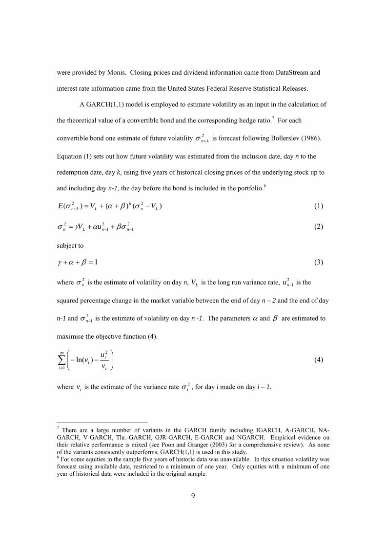
A GARCH(1,1) model is employed to estimate volatility as an input in the calculation of
the theoretical value of a convertible bond and the corresponding hedge ratio.7 For each
convertible bond one estimate of future volatility 2kn+σ is forecast following Bollerslev (1986).
Equation (1) sets out how future volatility was estimated from the inclusion date, day n to the
redemption date, day k, using five years of historical closing prices of the underlying stock up to
and including day n-1, the day before the bond is included in the portfolio.8
)()()( 22Ln
kLkn VVE −++=+ σβασ (1)
21
21
2−− ++= nnLn uV βσαγσ (2)
subject to
1=++ βαγ (3)
where 2nσ is the estimate of volatility on day n, LV is the long run variance rate, 2
1−nu is the
squared percentage change in the market variable between the end of day n – 2 and the end of day
n-1 and 21−nσ is the estimate of volatility on day n -1. The parameters α and β are estimated to
maximise the objective function (4).
∑=
⎟⎟⎠
⎞⎜⎜⎝
⎛−−
m
i i
ii v
uv
1
2
)ln( (4)
where iv is the estimate of the variance rate 2iσ , for day i made on day i – 1.
7 There are a large number of variants in the GARCH family including IGARCH, A-GARCH, NA-GARCH, V-GARCH, Thr.-GARCH, GJR-GARCH, E-GARCH and NGARCH. Empirical evidence on their relative performance is mixed (see Poon and Granger (2003) for a comprehensive review). As none of the variants consistently outperforms, GARCH(1,1) is used in this study. 8 For some equities in the sample five years of historic data was unavailable. In this situation volatility was forecast using available data, restricted to a minimum of one year. Only equities with a minimum of one year of historical data were included in the original sample.

10
In order to initiate a delta neutral hedge for each convertible bond we need to estimate the
delta for each convertible bond on the trading day it enters the portfolio. The delta estimate is
then multiplied by the convertible bond’s conversion ratio to calculate it∆ the number of shares
to be sold short in the underlying stock (the hedge ratio) to initiate the delta neutral hedge. On the
following day the new hedge ratio, 1+∆ it , is calculated, and if 1+∆ it > it∆ then 1+∆ it - it∆ shares
are sold, or if 1+∆ it < it∆ , then it∆ - 1+∆ it shares are purchased maintaining the delta neutral
hedge.9
Daily returns were calculated for each position on each trading day up to and including
the day the position is closed out. A position is closed out on the day the convertible bond is
delisted from the exchange. Convertible bonds may be delisted for several reasons. The
company may be bankrupt, the convertible may have expired or the convertible may have been
fully called by the issuer.
The returns for a position i on day t are calculated as follows.
Uitit
CBit
tititU
itU
itititCB
itCB
itit PP
SrDPPCPPR
111
1,1111 )(
−−−
−−−−−
∆+
++−∆−+−= (5)
Where itR is the return on position i at time t, CBitP is the convertible bond closing price at time t,
UitP is the underlying equity closing price at time t, itC is the coupon payable at time t, itD is the
dividend payable at time t, 1−∆ it is the delta neutral hedge ratio for position i at time t – 1 and
1,1 −− tit Sr is the interest on the short proceeds from the sale of the shares. Daily returns are then
compounded to produce a position value index for each hedged convertible bond over the entire
sample period.
9 As discussed earlier, due to transaction costs, an arbitrageur would not normally rebalance each hedge daily. However to avoid making ad hoc decisions on the timing of the hedge, we rebalance the portfolio daily and also exclude transaction costs.
11
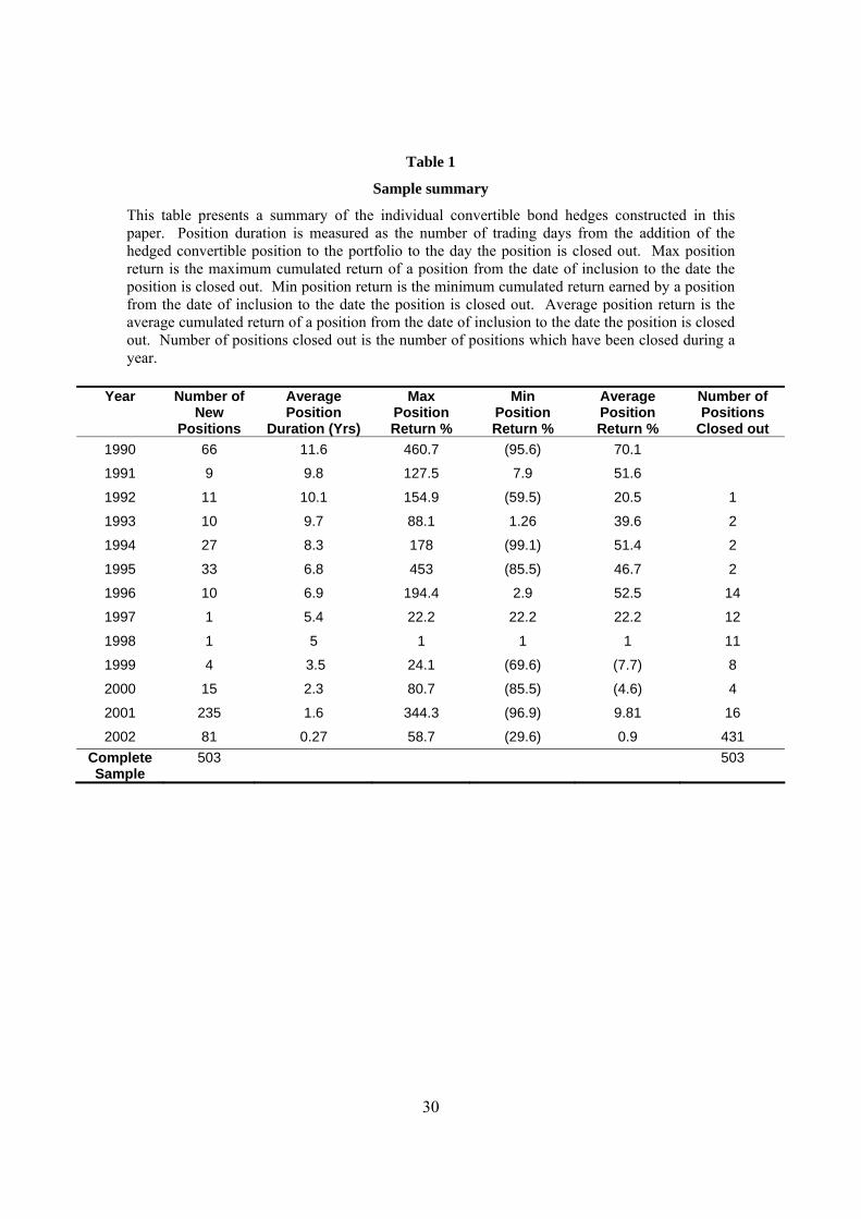
A summary of the individual convertible bond arbitrage return series is presented in
Table 1. The majority of new positions were added in the years 1990, 2001 and 2002.10 The
average position duration was 11.6 years, and the average position return was 70.1%, 4.7% per
annum. The maximum return on an individual position was 460.7% and the minimum position
return was -95.6%. 235 new positions were added in 2001, with average position duration of 1.6
years and average position return of 6% per annum. 1997, 1998 and 1999 are the years when the
fewest new positions were added to the portfolio. In 1997 and 1998 one new position was added
in each year, and in 1999 only four new positions were added. The lowest returns were generated
by positions added in 1999 and 2000, with average annual returns of -2.25% and -2%,
respectively. The closing out of positions is spread reasonably evenly over the sample period,
with the exception of 2002 where the majority of positions were closed out when the portfolio is
liquidated at 31st December 2002.
Two convertible bond arbitrage portfolios are calculated – an equally weighted and
market capitalisation weighted – using a similar methodology to CSFB Tremount Hedge Fund
Index (2002). As the market capitalisation portfolio has a bigger weighting of large convertible
bond issues it should be more liquid and be of a higher credit quality, thus intuitively one would
expect fewer arbitrage opportunities.
The value of the two convertible bond arbitrage portfolios on a particular date is given by
the formula.
t
Ni
iitit
t F
PVWV
t
∑=
== 1 (6)
where tV is the portfolio value on day t, itW is the weighting of position i on day t, itPV is the
value of position i on day t, tF is the divisor on day t and tN is the total number of position on day
10 In 1990, 66 new positions were added, of which 55 were listed prior to 1990.

12
t. For the equally weighted portfolio itW is set equal to one for each live hedged position. For
the market capitalization index the weighting for position j is calculated as follows.
∑=
=
=tNi
iit
jtjt
MC
MCW
1
(7)
where jtW is the weighting for position j at time t, tN is the total number of position on day t
and itMC is the market capitalization of issuer i at time t. To avoid daily rebalancing of the
market capitalization weighted portfolio the market capitalizations on the individual positions are
updated at the end of each calendar month. However, if a new position is added or an old
position is removed during a calendar month then the portfolio is rebalanced.
On the inception date of both portfolios, the value of the divisor is set so that the portfolio
value is equal to 100. Subsequently the portfolio divisor is adjusted to account for changes in the
constituents or weightings of the constituent positions in the portfolio. Following a portfolio
change the divisor is adjusted such that equation (8) is satisfied.
a
Ni
iiia
b
Ni
iiib
F
PVW
F
PVWtt
∑∑=
=
=
= = 11 (8)
Where iPV is the value of position i on the day of the adjustment, ibW is the weighting of position
i before the adjustment, ibW is the weighting of position i after the adjustment, bF is the divisor
before the adjustment and aF is the divisor after the adjustment.
Thus the post adjustment index factor aF is then calculated as follows.
∑
∑=
=
=
==t
t
Ni
iiia
Ni
iiibb
a
PVW
PVWxFF
1
1 (9)
13
As the margins on the strategy are small relative to the nominal value of the positions
convertible bond arbitrageurs usually employ leverage. Calamos (2003) and Ineichen (2000)
estimate that for an individual convertible arbitrage hedge fund this leverage may vary from one
to ten times equity. However, the level of leverage in a well run portfolio is not static and varies
depending on the opportunity set and risk climate. Khan (2002) estimates that in mid 2002
convertible arbitrage hedge funds were at an average leverage level of 2.5 to 3.5 times equity,
with estimates approximating 5 to 7 times equity in late 2001. In the case of our simulated
portfolios we apply leverage of one times equity to both our portfolios as this produces portfolios
with a similar average return to the HFRI Convertible Arbitrage Index and the CSFB Tremont
Convertible Arbitrage Index.11
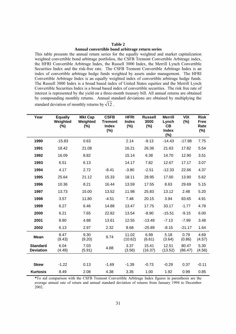
Table 2 presents annual return series for the equally weighted and market capitalization
weighted convertible bond arbitrage portfolios, the CSFB Tremont Convertible Arbitrage Index,
the HFRI Convertible Arbitrage Index, the Russell 3000 Index, the Merrill Lynch Convertible
Securities Index and the risk-free rate. The two highest returning years for the convertible bond
arbitrage portfolios, 1991 and 1995 correspond with the two highest returning years for the
Russell 3000, the Merrill Lynch convertibles index and the HFRI hedge fund index. In 1991 the
equally weighted index returned +17.2%, the market capitalization weighted index returned
17.43% and the HFRI index returned +16.2%. However, the convertible bond arbitrage strategy
was outperformed by a simple buy-and-hold equity (+26.4%) or convertible bond (+21.6%)
strategy. 1995 produced strong returns with the equally weighted portfolio +23.2%, the market
capitalization weighted portfolio +16.9%, the HFRI index +18.1% and the CSFB Tremont hedge
fund index +15.3%. Again the strategy was outperformed by a simple buy-and-hold equity
strategy (+29%) but outperformed the general convertible securities market.
11 To ensure the level of leverage is not an important factor in our results we apply alternative levels of leverage to the portfolio from 0 to 5 times. Results were not materially different than for the 1 times equity portfolio and are available from the authors.
14
The lowest returns for the equally weighted convertible bond arbitrage portfolio occur in
1990 and 1994, which also corresponds with negative returning years for the Russell 3000 and
Merrill Lynch convertible securities index.12 The HFRI index had a below average return of
+2.14% in 1990 and had its lowest return of -3.8% in 1994. The CSFB Tremont index does not
date back to 1990 but in 1994 it had also had its lowest return of -8.4%. The two lowest returning
years for the market capitalization weighted index were 1990 and 1992. In 1998 the CSFB
Tremont index also had a negative return of -4.5%, however none of the other indices or
portfolios had negative returns.
More recently in 2000, 2001 and 2002, after the bursting of the dotcom bubble, both of
the convertible bond arbitrage portfolios (returning an average 7.3% for the equally weighted and
5.52% for the market capitalization weighted), the HFRI Convertible Arbitrage Index and the
CSFB Tremont Convertible Arbitrage Hedge Fund Index have performed well. During this
period the Russell 3000 and the Merrill Lynch Convertible Securities Index had an average
annual return of -16.1% and -10.26%. This performance has demonstrated the diversification
benefits of the convertible bond arbitrage strategy. However, it should be noted that the sample
period has been characterized by rapidly falling interest rates and an increase in convertible
issuance.
Looking at the distribution of the monthly returns, both the equal weighted and the
market capitalization weighted portfolios display negative skewness of -1.23 and -0.77,
respectively. The CSFB Tremont index and the HFRI index also display negative skewness.
This is consistent with other studies (see Agarwal and Naik, 2004; Kat and Lu, 2002). The
monthly returns from the equal weighted and the market capitalization weighted portfolios also
display positive kurtosis. Similar to Kat and Lu (2002), we find that the estimates of kurtosis
appear to be high relative to the two hedge fund indices.
12 Ineichen (2000) notes that 1994 was not a good year for convertible arbitrage characterised by rising US interest rates.
15
3. Validation of Convertible Arbitrage Portfolios
A comparison of the convertible bond arbitrage portfolios with two market standard
hedge fund indices and the overall market portfolio for a variety of market conditions provides a
starting point in validating the robustness of the two generated portfolios. Furthermore, as
highlighted earlier, investors have become interested in lower volatility non-directional arbitrage
strategies because of the diversification benefits they bring to their portfolios in a low-return
equity environment. A comparison across market conditions provides evidence of this
diversification benefit dependence to market swings.
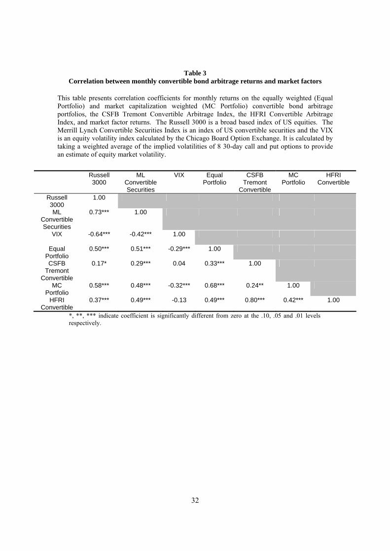
Table 3 presents the correlation coefficients between the monthly returns on the equally
weighted convertible bond arbitrage portfolio (Equal), the market capitalization weighted
portfolio (MC), the CSFB Tremont Convertible Arbitrage Index (CSFB), the HFRI Convertible
Arbitrage Index (HFRI), the Russell 3000, the Merrill Lynch Convertible Securities Index
(MLCS) and the VIX Index (VIX)13. As the CSFB data is unavailable prior to 1994 the
correlation coefficients cover returns from January 1994 to December 2002.14
The Equal, MC, CSFB and HFRI indices are all positively correlated with the MLCS
index. With the exception of the CSFB index they are also all positively correlated with equities.
The Equal is positively correlated with the MC, CSFB and HFRI indices over the entire sample
period. Surprisingly, the MC is not correlated with the CSFB index, although it is positively
correlated with the HFRI index. Monthly returns on the VIX are negatively correlated with both
the Equal and MC portfolios indicating that they are both negatively correlated with implied
volatility. Neither of the hedge fund indices has any correlation with the VIX. This is surprising
as convertible bond arbitrage is a long volatility strategy.
13 The VIX index is an equity volatility index calculated by the Chicago Board Option Exchange. It is calculated by taking a weighted average of the implied volatilities of 8 30-day call and put options to provide an estimate of equity market volatility. 14 Correlation coefficients were estimated for the entire sample period 1990 to 2002 for all variables excluding the CSFB data. There was no change in the sign or significance of any of the coefficients.
16
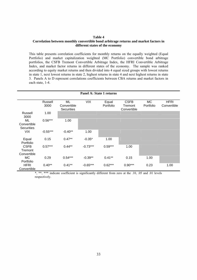
Next we ranked our sample of 108 monthly returns by equity market return and
subdivided the sample into four equal sized sub-samples of 27 months. State 1, which is
presented in Panel A of Table 4, covers the correlations between convertible bond arbitrage
returns and market factors in the 27 lowest equity market returns (ranging from -16.8% to -2.6%).
The Equal portfolio and the two hedge fund indices are positively correlated with the MLCS
index in this sub-sample. The Equal portfolio is positively correlated with the two hedge fund
indices and the three are all negatively correlated with the VIX. In this sub-sample the MC
portfolio is not correlated with any of the other return series or market factors. The Equal
portfolio shares more characteristics with the hedge fund indices, than the MC portfolio does.
Panel B of Table 4 looks at the correlations between convertible bond arbitrage returns
and market factors in the 27 next lowest equity market returns (ranging from -2.2% to +1.3%).
None of our convertible arbitrage portfolios or indices has any correlation with equities in this
sub-sample. Both the CSFB and HFRI indices are correlated with the MLCS and VIX indices.
The Equal portfolio is positively correlated with the MC portfolio and also the two hedge fund
indices are positively correlated.
Panel C of Table 4 looks at the correlations between convertible arbitrage returns and
market factors in the 27 next lowest equity market returns (ranging from +1.4% to +3.9%). The
two hedge fund indices are positively correlated with the MLCS index and each other. The MC
portfolio is also correlated with the HFRI index.
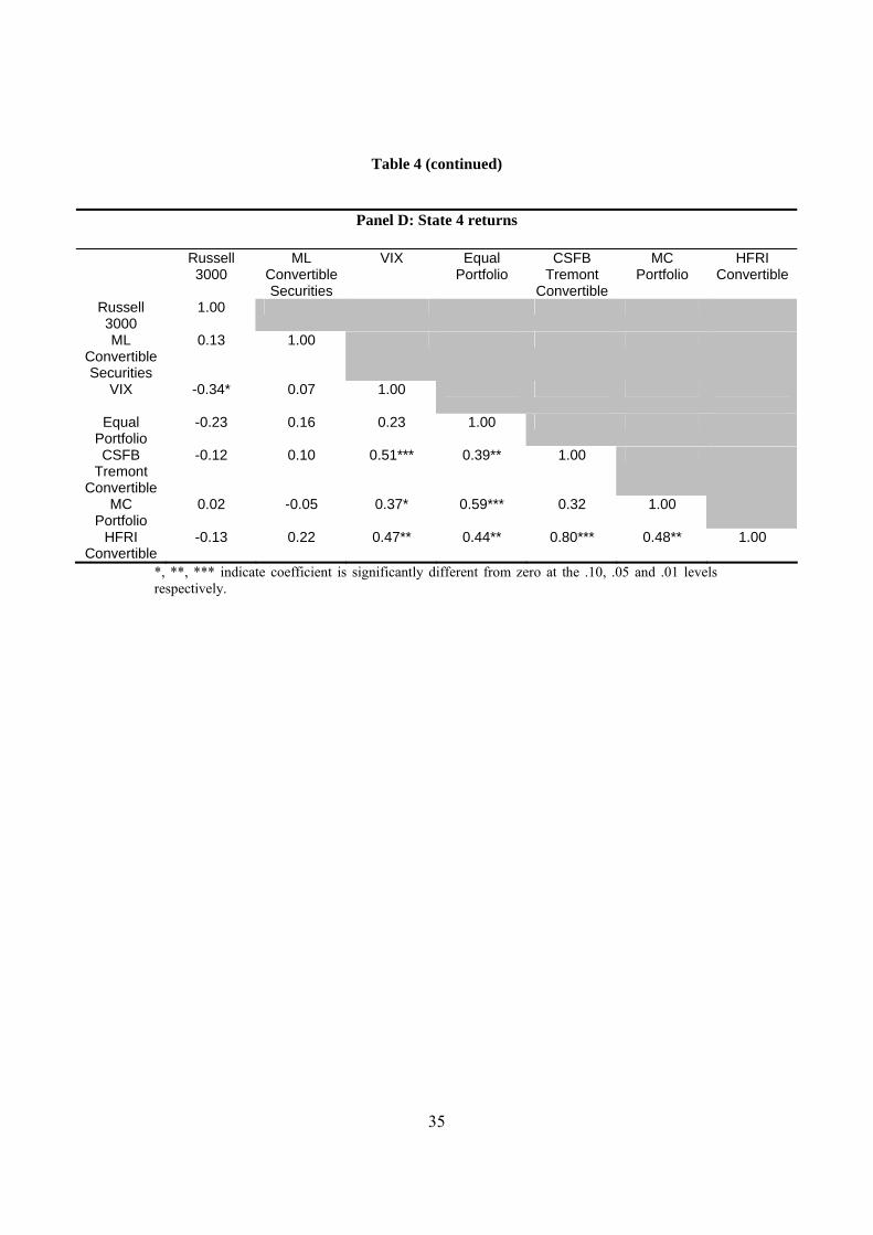
The final sub-sample, looking at the correlations between convertible arbitrage returns
and market factors in the 27 highest equity market returns (ranging from +4.0% to 7.6%) is
presented in Panel D of Table 4. The Equal portfolio is positively correlated with the MC
portfolio and the HFRI index. Both the CSFB and HFRI indices are positively correlated with the
VIX in this sample period.
Based on the evidence presented in this section the two hedge fund indices appear to
share many of the characteristics of our convertible bond arbitrage portfolios. Over the entire
17
sample period they are all positively correlated, and when the sample is subdivided they share
similar characteristics.
4. Convertible bond arbitrage performance measurement
Prior analysis of convertible bond arbitrage in the literature has highlighted the perceived
abnormal positive risk adjusted returns that the strategy generates. Ineichen (2000) uses a linear
one factor model to document the abnormal returns generated by convertible arbitrage hedge fund
indices. More recently, Capocci and Hübner (2004), utilising a linear specification, document
convertible arbitrage funds exhibiting significant positive abnormal returns using both single
factor and multi factor models. Regardless of the performance measure, model or sample
employed convertible bond arbitrage exhibit a significant positive abnormal return (Kazemi and
Schneeweis, 2003).
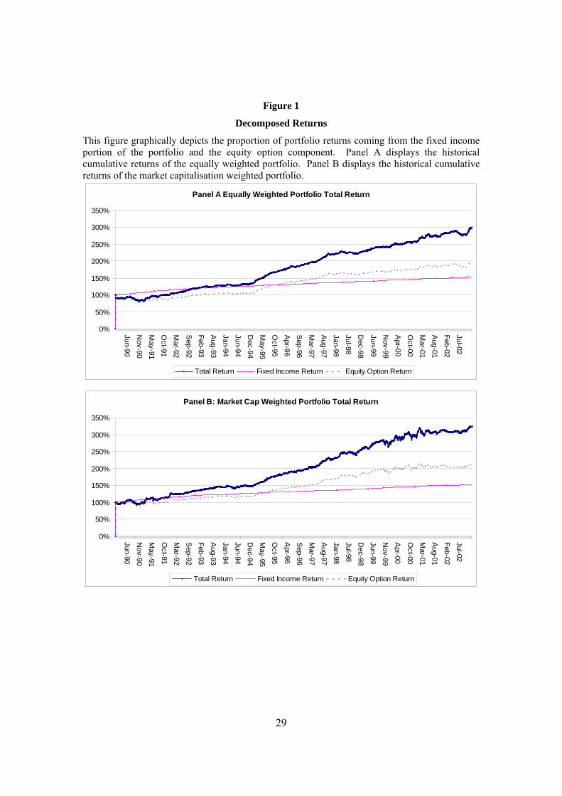
To aid the definition of appropriate risk factors we first decompose the returns of the two
convertible arbitrage portfolios into their fixed income and equity option components.15 Figure 1
graphically displays the proportion of total returns derived from each of these sources for the
equally weighted and market capitalisation weighted portfolios. For the equally weighted
(market capitalisation weighted in parenthesis) portfolio which has an average annual return of
8.5% (9.3%) the fixed income component contributes 3.2% (3.0%) with the balance of 5.4%
(6.3%) coming from the equity option component. As can be seen graphically the annualised
standard deviation of the fixed income component is lower, 0.8% (0.8%), than the equity option
component with an annualised standard deviation of 5.61% (6.6%).
Given this evidence we specify four asset pricing models using combinations of equity
and bond market factors to isolate the convertible arbitrage data generating process: the market
model derived from the Capital Asset Pricing Model (CAPM) described in Sharpe (1964) and
Lintner (1965), the Fama and French (1993) three factor stock model, the Fama and French 15 We are grateful to an anonymous reviewer for this suggestion.
18
(1993) three factor bond model and the Fama and French (1993) combined stock and bond model.
Below we briefly review these models, providing an explanation of the expected relationship
between convertible arbitrage returns and the individual factors.
The market model is a single index model which assumes that all of a stock’s systematic
risk can be captured by one market factor. The intercept of the equation, α, is commonly called
Jensen’s (1968) alpha and is usually interpreted as a measure of out- or under-performance. The
equation to estimate is the following:
RCB - Rf = α +βRMRFRMRF + εt (10)
Where yt = Rt – Rft , Rt is the return on the hedge fund index at time t, Rft is the risk free
rate at month t (the yield on a one month treasury bill), RMRFt is the excess return on the market
portfolio (here the Russell 3000 is specified as a market proxy) on month t, is the error term α
and βRMRF are the intercept and the slope of the regression, respectively. As convertible
arbitrageur’s are exposed to equity option risk there should be a significantly positive βMKT
coefficient.
The Fama and French (1993) three factor stock model is estimated from an expected form
of the CAPM model. This model extends the CAPM with the inclusion of two factors which take
the size and market to book ratio of firms into account. It is estimated from the following
equation:
RCB - Rf = α +βRMRFRMRF + βSMBSMB + βHMLHML + εt (11)
Where SMBt is the factor mimicking portfolio for size (small minus big) at time t and
HMLt is the factor mimicking portfolio for book to market ratio (high minus low) at time t.16
Capocci and Hübner (2004) specify the HML and SMB factors in their models of hedge fund
16 For details on the construction of SMB and HML see Fama and French (1992, 1993).
19
performance. Agarwal and Naik (2004) specify the SMB factor in a model of convertible
arbitrage performance and find it has a positive relation with convertible arbitrage returns. As the
opportunities for arbitrage are greater in the smaller less liquid issues ex ante it would be
expected that a positive relationship between convertible arbitrage returns and the size factor.
There is no ex ante expectation of the relationship between the factor mimicking for book to
market equity and convertible arbitrage returns though Capocci and Hübner (2004) report a
positive HML coefficient for convertible arbitrage.
Fama and French (1993) also propose a three factor model for the evaluation of bond
returns. They draw on Chen et al. (1986) to extend the CAPM incorporating two additional
factors taking the shifts in economic conditions that change the likelihood of default and
unexpected changes in interest rates into account. This model is estimated from the following
equation
RCB - Rf = α +βRMRFRMRF + βDEFDEF + βTERMTERM + εt (12)
Where DEFt is the difference between the overall return on a market portfolio of long-
term corporate bonds17 minus the long term government bond return at month t18. TERMt is the
factor proxy for unexpected changes in interest rates. It is constructed as the difference between
monthly long term government bond return and the short term government bond return19. It is
expected that convertible arbitrage returns will be positively related to both of these factors as the
strategy generally has term structure and credit risk exposure.
17 The return on the DataStream Index of high yield corporate bonds is specified rather than the return on the composite portfolio from Ibbotson and Associates used by Fama and French (1993) due to its unavailability. 18 The return on the DataStream Index of long term government bonds is specified rather than the return on the monthly long term government bond return from Ibbotson and Associates used by Fama and French (1993) due to its unavailability. 19 The return on the DataStream Index of short term government bonds is specified rather than the one month treasury bill rate used by Fama and French (1993).
20
Fama and French (1993) also estimate a combined model when looking at the risk factors
affecting stock and bond returns. As a convertible bond is a hybrid bond and equity instrument
we also estimate this model using the following combined model:
RCB - Rf = α +βRMRFRMRF + βSMBSMB + βHMLHML + βDEFDEF + βTERMTERM + εt (13)
To correct for the potential downward bias in beta estimation when using daily
convertible bond data two lags of the daily return on each of the risk factors are specified in
addition to the contemporaneous return when estimating (10) to (13). This downward bias is
caused by non-synchronous trading between the illiquid convertible bonds and the more liquid
asset class factors.20
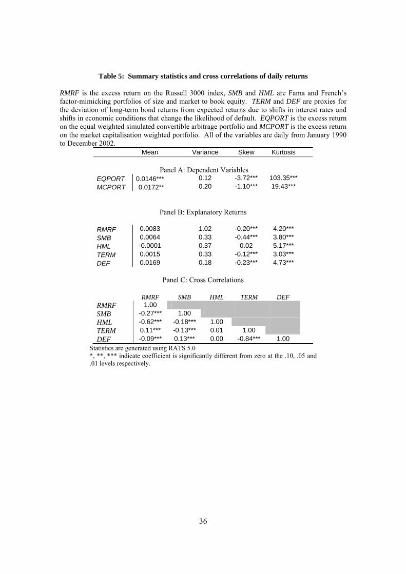
Table 5, Panel B presents summary statistics of the daily explanatory factor returns.21
None of the risk factors have average returns significantly different from zero. RMRF has the
largest variance and four of the factors, RMRF, SMB, TERM and DEF exhibit significant negative
skewness at the 1% level. All of the factors exhibit significant excess kurtosis. Table 5, Panel C
presents a correlation matrix of the explanatory variables daily returns. There is a high absolute
correlation between two of the equity market factors, RMRF and HML, and the bond factors
TERM and DEF. In the next section we report results from estimating the relationship between
the simulated portfolio returns and these risk factors.
5. Results of the asset class factor model regressions
In this section, the results of estimating the risk factor models defined in the previous
section on the simulated convertible arbitrage portfolio are presented. We also present empirical 20 Scholes and Williams (1977) and Dimson (1979) amongst others show that betas of securities that trade less (more) frequently than the index used as the market proxy are downward (upward) biased. 21 Data on SMB and HML was provided by Kenneth French.
21
evidence supporting our hypothesis of non-linearity in the relationship between simulated
portfolio returns and risk factors.
Table 6 presents results of the OLS estimation of the risk factor models discussed above
for the equally weighted convertible bond arbitrage portfolio. Although the conditional
heteroskedasticity and autocorrelation are not formally treated in the OLS estimate of the
parameters, the test statistics are heteroskedasticity and autocorrelation consistent due to Newey
and West (1987). As discussed above contemporaneous observations and two lags are specified
for each risk factor. The β coefficients are the sum of the contemporaneous β and lagged β s. P-
values from testing the general linear restrictions that α = 0 and (βit + βit-1 + βit-2 ) = 0, for i =
RMRF, SMB, HML, DEF and TERM are in parenthesis.
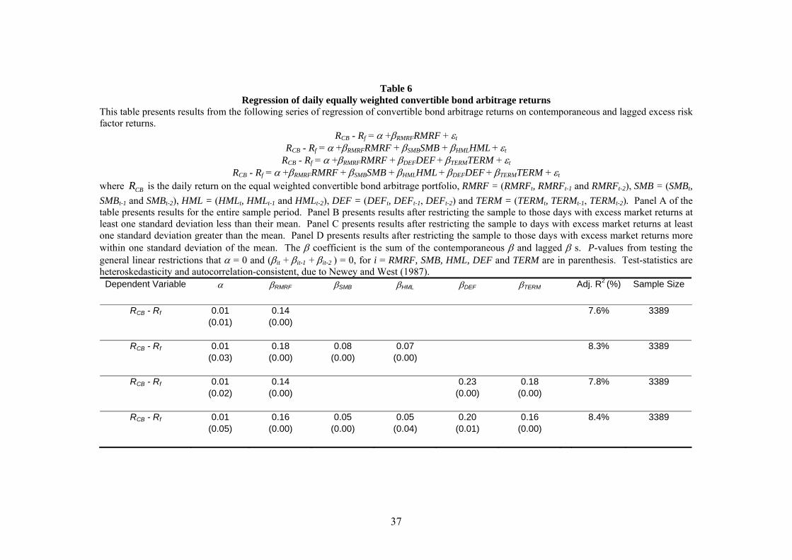
The first reported results are for the market model. The market coefficient value of 0.14
is significantly positive indicating that there is a positive relationship between convertible bond
arbitrage returns and the market portfolio. This is a finding consistent with Capocci and Hübner
(2004) who estimate a significantly positive market coefficient for convertible arbitrage hedge
funds of 0.06. The second result is from estimation of the Fama and French (1993) three factor
stock model. The factor loadings on all three factors are significantly positive, consistent with
Capocci and Hübner’s (2004) findings for convertible arbitrage. The penultimate result is from
estimation of the Fama and French (1993) bond factor model. The coefficients on both factors,
DEF and TERM, are highly significant, with coefficient weightings greater than 0.20. The final
result is an estimation of the combined Fama and French’s (1993) bond and stock factor models.
The coefficients for RMRF, SMB, HML, DEF and TERM are all significantly different from zero.
Estimated alphas from the four models are all significantly positive at, at least the 5%
significance level.
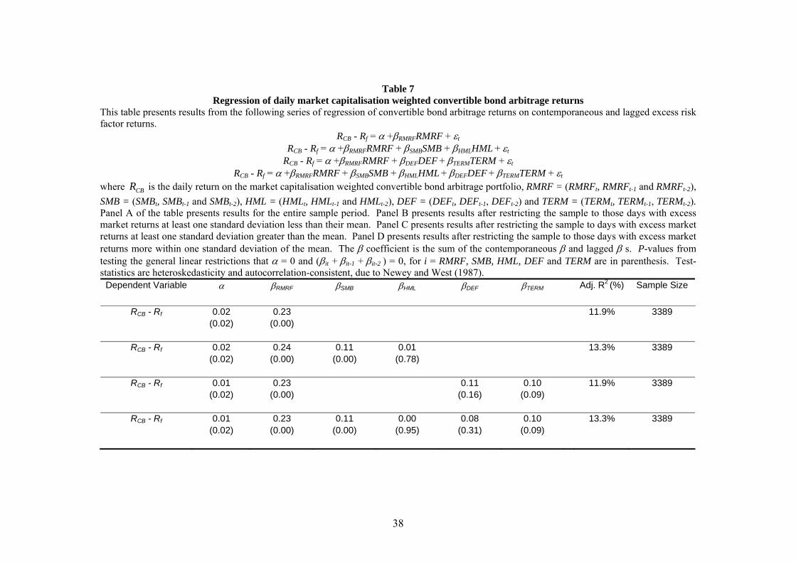
Table 7 reports similar results for the market capitalisation weighted index. Factor
loadings on equity market risk factors are larger than for the equal weighted portfolio. This is
22
unsurprising given the market capitalisation weighted portfolio derives a larger proportion of
returns from the equity option component than the equal weighted portfolio. Estimated alphas
from the four models are all significantly positive at the 5% significance level.
The results reported in Tables 6 and 7 provide evidence that the convertible bond
arbitrage strategy has significant risk exposure to both equity and bond market factors. As a
larger proportion of returns are derived from the higher variance equity option component these
factors explain a large proportion of returns in a linear framework. Nonetheless, the bond market
factors are also highly significant.
Next we investigate non-linearity in the relationship between these risk factors and the
simulated portfolio returns. Agarwal and Naik (2004) document that convertible bond arbitrage
hedge funds exhibit written naked put option like returns, with a stronger correlation between the
returns of convertible arbitrage hedge fund indices and equities in down markets. This finding is
inconsistent with theoretical expectations. The convertible bond is a hybrid bond and equity
instrument. As the underlying equity price decreases we expect the delta of the convertible to fall
and it to become more bond and less equity like. We would expect to find a decrease in equity
market risks and an increase in fixed income risks under these conditions.
To investigate this we rank and subdivide the sample by historical equity market returns.
We estimate the combined equity and bond performance measurement model (13) for the equally
weighted and market capitalisation weighted portfolios in three sub-samples. First, in weak
equity markets, when the excess market return is at least one standard deviation less than the
mean; second, in strong equity markets, when the excess market return is at least one standard
deviation greater than the mean; and, finally in benign equity markets, when the excess market
return is within one standard deviation of the mean.
Table 8 reports the results of OLS estimation of the risk factor model for the three sub-
samples. (To aid comparison the full sample regression from Table 6 is also reported in Panel A.)
There are three main results to note from this table. Panel B reports results after restricting the
23
sample to those days where the excess market return is at least one standard deviation less than
the mean. First, Note the increase in coefficient values for the bond market factors and the
decrease in coefficients and significance for the equity market factors. Second, note the decrease
in coefficient values and significance for the bond market factors, DEF and TERM in Panel C the
results for the sub-sample at least one standard deviation greater than the mean. Finally, the
estimated alphas in each of these sub-samples are not significantly different from zero.
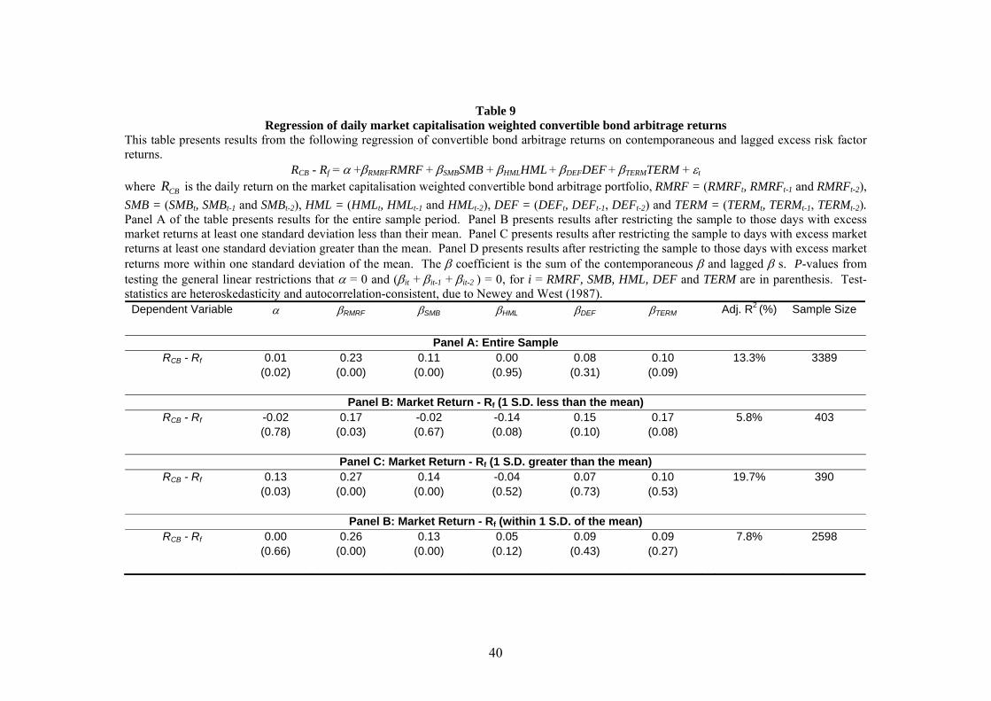
Table 9 reports a similar set of results for the market capitalisation weighted portfolio.
Again the DEF and TERM coefficients increase in magnitude and significance when stock returns
are low. The equity related coefficients decrease in this sub-sample and increase in size and
significance when equity returns are at least one standard deviation greater than the mean. In
Table 9 only the alpha estimated in Panel C (equity market returns at least one standard deviation
greater than the mean) is significantly positive.
These results provide more evidence on the risks in the convertible arbitrage strategy.
The strategy is exposed to both equity and bond market risk factors but these risk exposures are
non-stationary. When equity market returns are weak the aggregate delta of the convertibles in
the portfolio falls and the portfolio is more exposed to default and term structure risk factors.
When equity market returns are high the aggregate delta of the bonds increases and the portfolios
equity market risk exposure increases. Failing to correct for this inherent non-linearity can lead
to erroneous conclusions on performance. The estimated alphas reported in Tables 8 and 9 are
only significant in rising equity markets and only for the market capitalisation weighted portfolio.
These results contrast with the linear full sample model in Table 6 and 7 with estimated alphas
significantly positive irrespective of the performance measurement model specified.
6. Conclusion
In this paper we simulate a convertible bond arbitrage portfolio providing evidence on the
characteristics of this dynamic trading strategy. As this simulated portfolio is free of the biases

24
found in self reported hedge fund data, it serves as a useful benchmark to evaluate the risks and
performance of the strategy.
We combine long positions in convertible bonds with short positions in the common
stock of the issuer to create individual delta neutral hedged convertible bonds in a manner
consistent with an arbitrageur capturing income. These individual positions are then dynamically
hedged on a daily basis to capture volatility and maintain a delta neutral hedge. We then combine
these positions into two convertible bond arbitrage portfolios and demonstrate that the monthly
returns of our convertible bond arbitrage portfolio are positively correlated with two indices of
convertible arbitrage hedge funds.
Next we decompose the returns of these portfolios into fixed income and equity option
components aiding the definition of a set of appropriate risk factors. We provide evidence that
the portfolios have statistically significant positive relationships with excess equity returns, a size
factor and default and term structure risk factors. We also include a book-to-market factor which
has a weaker relationship with portfolio returns. Results of these different linear asset class factor
models suggest the strategy generates superior risk adjusted returns.
To investigate the findings of Agarwal and Naik (2004), that convertible arbitrage has an
increase in equity market risk in depreciating markets we investigate for non-linearity in the
relationship between simulated portfolio returns and the bond and equity market risk factors.
Consistent with theoretical expectations we find that equity related risk coefficients increase and
decrease in appreciating and depreciating equity markets respectively. Likewise, bond related
risk coefficients decrease and increase in appreciating and depreciating equity markets
respectively. Correcting for this non-linearity eliminates the perceived abnormal risk adjusted
performance of the portfolios.22
22 With the exception of the market capitalisation weighted portfolio in the appreciation equity markets sub-sample.
25
References
Agarwal, V. and N.Y. Naik (2004), ‘Risks and Portfolio Decisions Involving Hedge Funds’,
Review of Financial Studies, Vol.17, No.1 (Spring), pp. 63-98.
Ammann, M., A. Kind and C. Wilde (2004), ‘Are Convertible Bonds Underpriced? An Analysis
of the French Market’, Journal of Banking and Finance, Vol.27, No.4 (April), pp. 635-653.
Barkely, T. (2001), ‘Hedge Funds Drive Convertible-Bond Demand as Starwood Launches it’s
$500 Million Issue, Wall Street Journal, May 8.
BIS, (2004), BIS Quarterly Review, March (Bank of International Settlement Publication).
Bollerslev, T. (1986), ‘Generalised Autoregressive Heteroskedasticity’, Journal of Econometrics
Vol.31, No.3 (April), pp.307-327.
Calamos, N. (2003), ‘Convertible Arbitrage: Insights and Techniques for Successful Hedging’,
(New Jersey: John Wiley and Sons).
Capocci, D. and G. Hübner (2004), ‘Analysis of Hedge Fund Performance’ Journal of Empirical
Finance Vol.11, No. 1 (January), pp. 55-89.
Chen N-F, R. Roll and S. Ross (1986), ‘Economic Forces and the Stock Market’, Journal of
Business, Vol. 59, No. 3 (July), pp. 383-403.
CSFB Tremont (2002), ‘CSFB/Tremont Hedge Fund Index: Index Construction Rules’,
www.hedgeindex.com.
Dimson, E. (1979), ‘Risk Measurement when Shares are Subject to Infrequent Trading’, Journal
of Financial Economics, Vol.7, No. 2 (June), pp. 197-226.
Fama E.F. and K.R. French. (1992), ‘The Cross-Section of Expected Stock Returns’, Journal of
Finance, Vol. 47, No. 2 (June), pp. 427-465
26
(1993), ‘Common Risk Factors in the Returns on Stocks and Bonds’, Journal of
Financial Economics, Vol. 33, No. 1 (February), pp. 3-56
Fortune (1966), ‘Personal Investing: those Fantastic ‘Hedge Funds’’, April, Fortune Magazine.
Fung, W. and D.A. Hsieh (1997), ‘Empirical Characteristics of Dynamic Trading Strategies: the
Case of Hedge Funds’, Review of Financial Studies, Vol. 10, No. 2 (Summer), pp. 275–302.
(2000a), ‘Measuring the Market Impact of Hedge Funds’, Journal of Empirical
Finance Vol.7, No. 1 (May), pp. 1–36.
(2000b), ‘Performance Characteristics of Hedge Funds: Natural vs. Spurious Biases’,
Journal of Financial and Quantitative Analysis, Vol.35, No. 3 (September), pp. 291–307.
(2001), ‘The Risk in Hedge Fund Trading Strategies: Theory and Evidence from
Trend Followers’, Review of Financial Studies, Vol. 14, No. 2 (Summer), pp. 313–341.
(2002), ‘Risk in Fixed-Income Hedge Fund Styles’, Journal of Fixed Income, Vol. 12,
No. 2 (September), pp. 1–22.
Getmansky M., A.W. Lo and I. Makarov (2004), ‘An Econometric Model of Serial Correlation
and Illiquidity in Hedge Fund Returns’, Journal of Financial Economics, Vol.74, No.3
(December), pp. 529-609.
Ineichen, A. (2000) In Search of Alpha (United Kingdom: UBS Warburg Research Publication).
Kang, J.K. and Y.W Lee (1996), ‘The Pricing of Convertible Debt Offerings’, Journal of
Financial Economics, Vol.41, No. 2 (June), pp.231-248.
Kat, H.M. and S. Lu (2002), ‘An Excursion into the Statistical Properties of Hedge Funds’,
Working Paper (CASS Business School).
Kazemi, H. and T. Schneeweis (2003), ‘Conditional Performance of Hedge Funds’, CISDM
Working Paper, Isenberg School of Management, University of Massachusetts, Amherst, March.
27
Khan, S.A. (2002), ‘A Perspective on Convertible Arbitrage’, Journal of Wealth Management,
Vol. 5, No. 2 (Fall), pp. 59–65.
King, R. (1986), ‘Convertible Bond Valuation: an Empirical Test’, Journal of Financial Research
Vol.9, No. 1 (March), pp. 53-69.
Liang, B. (1999), ‘On the Performance of Hedge Funds’, Financial Analysts Journal, Vol. 55,
No. 4 (July/August), pp. 72-85.
(2000), ‘Hedge funds: the living and the dead’, Journal of Financial and Quantitative
Analysis, Vol. 35, No. 3 (September), pp. 72-85.
Lintner J. (1965), ‘The Valuation of Risk Assets and the Selection of Risky Investments in Stock
Portfolio and Capital Budgets’, Review of Economics and Statistics Vol. 47, No. 1 (February), pp.
13-37.
McGee (2003), ‘Extra fuel’, http://www.financial-planning.com/pubs/fp/20031201028.html
Mitchell, M. and T. Pulvino, (2001), ‘Characteristics of Risk and Return in Risk Arbitrage’,
Journal of Finance, Vol. 56, No. 6 (December), pp. 2135-2175.
Newey W.K. and K.D. West (1987), ‘A Simple, Positive Semi-definite Heteroskedasticity and
Autocorrelation Consistent Covariance Matrix’, Econometrica, Vol. 55, No. 3 (May), pp. 707-
708.
Poon, S.-H. and C. Granger (2003), ‘Forecasting Volatility in Financial Markets: a Review’,
Journal of Economic Literature, Vol. 41, No. 2 (June), pp. 478-539.
Schneeweis, T. and R. Spurgin (1998), ‘Multifactor Analysis of Hedge Funds, Managed Futures
and Mutual Fund Return and Risk Characteristics’, Journal of Alternative Investments Vol. 1, No.
2 (Fall), pp.1-24.
28
Scholes, M. and J.T. Williams (1977), ‘Estimating Betas from Nonsynchonous Data’, Journal of
Financial Economics, Vol. 5, No. 3 (December), pp. 309-327.
Sharpe W.F. (1964), ‘Capital Asset Prices: A Theory of Market Equilibrium under Conditions of
Risk’, Journal of Finance, Vol. 19, No. 3 (September), pp. 425-442
(1966), ‘Mutual Fund Performance’, Journal of Business, Vol. 39, No. 1 (January), pp. 119-
138.
(1992), ‘Asset Allocation: Management Style and Performance Measurement’, Journal of
Portfolio Management, Vol. 18, No. 1 (Winter), pp. 7-19.
29
Figure 1
Decomposed Returns
This figure graphically depicts the proportion of portfolio returns coming from the fixed income portion of the portfolio and the equity option component. Panel A displays the historical cumulative returns of the equally weighted portfolio. Panel B displays the historical cumulative returns of the market capitalisation weighted portfolio.
Panel A Equally Weighted Portfolio Total Return
0%
50%
100%
150%
200%
250%
300%
350%
Jun-90N
ov-90M
ay-91
Oct-91
Mar-92
Sep-92
Feb-93
Aug-93
Jan-94Jun-94
Dec-94
May-95
Oct-95
Apr-96
Sep-96
Mar-97
Aug-97
Jan-98Jul-98
Dec-98
Jun-99N
ov-99A
pr-00
Oct-00
Mar-01
Aug-01
Feb-02Jul-02
Total Return Fixed Income Return Equity Option Return
Panel B: Market Cap Weighted Portfolio Total Return
0%
50%
100%
150%
200%
250%
300%
350%
Jun-90
Nov-90
May-91
Oct-91
Mar-92
Sep-92
Feb-93
Aug-93
Jan-94
Jun-94
Dec-94
May-95
Oct-95
Apr-96
Sep-96
Mar-97
Aug-97
Jan-98
Jul-98
Dec-98
Jun-99
Nov-99
Apr-00
Oct-00
Mar-01
Aug-01
Feb-02
Jul-02
Total Return Fixed Income Return Equity Option Return
30
Table 1
Sample summary
This table presents a summary of the individual convertible bond hedges constructed in this paper. Position duration is measured as the number of trading days from the addition of the hedged convertible position to the portfolio to the day the position is closed out. Max position return is the maximum cumulated return of a position from the date of inclusion to the date the position is closed out. Min position return is the minimum cumulated return earned by a position from the date of inclusion to the date the position is closed out. Average position return is the average cumulated return of a position from the date of inclusion to the date the position is closed out. Number of positions closed out is the number of positions which have been closed during a year.
Year Number of New
Positions
Average Position
Duration (Yrs)
Max Position Return %
Min Position Return %
Average Position Return %
Number of Positions
Closed out 1990 66 11.6 460.7 (95.6) 70.1
1991 9 9.8 127.5 7.9 51.6
1992 11 10.1 154.9 (59.5) 20.5 1
1993 10 9.7 88.1 1.26 39.6 2
1994 27 8.3 178 (99.1) 51.4 2
1995 33 6.8 453 (85.5) 46.7 2
1996 10 6.9 194.4 2.9 52.5 14
1997 1 5.4 22.2 22.2 22.2 12
1998 1 5 1 1 1 11
1999 4 3.5 24.1 (69.6) (7.7) 8
2000 15 2.3 80.7 (85.5) (4.6) 4
2001 235 1.6 344.3 (96.9) 9.81 16
2002 81 0.27 58.7 (29.6) 0.9 431 Complete Sample
503 503
31
Table 2 Annual convertible bond arbitrage return series
This table presents the annual return series for the equally weighted and market capitalization weighted convertible bond arbitrage portfolios, the CSFB Tremont Convertible Arbitrage index, the HFRI Convertible Arbitrage Index, the Russell 3000 Index, the Merrill Lynch Convertible Securities Index and the risk-free rate. The CSFB Tremont Convertible Arbitrage Index is an index of convertible arbitrage hedge funds weighted by assets under management. The HFRI Convertible Arbitrage Index is an equally weighted index of convertible arbitrage hedge funds. The Russell 3000 Index is a broad based index of United States equities and the Merrill Lynch Convertible Securities Index is a broad based index of convertible securities. The risk free rate of interest is represented by the yield on a three-month treasury bill. All annual returns are obtained by compounding monthly returns. Annual standard deviations are obtained by multiplying the standard deviation of monthly returns by 12 .
Year Equally Weighted
(%)
Mkt Cap Weighted
(%)
CSFB Tremont
Index (%)
HFRI Index (%)
Russell 3000 (%)
Merrill Lynch
CB Index (%)
VIX (%)
Risk Free Rate (%)
1990 -15.83 0.63 2.14 -9.13 -14.43 -17.98 7.75
1991 18.42 21.08 16.21 26.36 21.63 17.82 5.54
1992 16.09 8.82 15.14 6.38 14.70 12.90 3.51
1993 6.51 6.13 14.17 7.82 12.67 17.17 3.07
1994 4.17 2.72 -8.41 -3.80 -2.51 -12.33 22.66 4.37
1995 25.64 21.12 15.33 18.11 28.95 17.00 13.90 5.62
1996 10.36 8.21 16.44 13.59 17.55 8.63 29.69 5.15
1997 13.73 15.00 13.52 11.98 25.83 13.12 2.48 5.20
1998 3.57 11.80 -4.51 7.48 20.15 3.94 83.65 4.91
1999 6.27 6.46 14.88 13.47 17.75 33.17 -1.77 4.78
2000 6.21 7.65 22.82 13.54 -8.90 -15.51 -9.15 6.00
2001 8.80 4.88 13.61 12.55 -13.49 -7.13 -7.99 3.48
2002 6.13 2.97 2.32 8.68 -25.89 -8.15 -21.17 1.64
Mean 8.47 (9.43)
9.30 (9.20) 9.74 11.02
(10.62) 6.99
(6.61) 5.18
(3.64) 0.79
(0.86) 4.69
(4.57)
Standard Deviation
6.04 (4.48)
7.03 (5.91) 4.88 3.37
(3.56) 15.41
(16.37) 12.51
(13.52) 80.47
(86.47) 5.30
(4.56)
Skew -1.22 0.13 -1.69 -1.39 -0.73 -0.29 0.37 -0.11
Kurtosis 8.49 2.08 4.38 3.35 1.00 1.92 0.99 0.85 *To aid comparison with the CSFB Tremont Convertible Arbitrage Index figures in parenthesis are the average annual rate of return and annual standard deviation of returns from January 1994 to December 2002.
32
Table 3 Correlation between monthly convertible bond arbitrage returns and market factors
This table presents correlation coefficients for monthly returns on the equally weighted (Equal Portfolio) and market capitalization weighted (MC Portfolio) convertible bond arbitrage portfolios, the CSFB Tremont Convertible Arbitrage Index, the HFRI Convertible Arbitrage Index, and market factor returns. The Russell 3000 is a broad based index of US equities. The Merrill Lynch Convertible Securities Index is an index of US convertible securities and the VIX is an equity volatility index calculated by the Chicago Board Option Exchange. It is calculated by taking a weighted average of the implied volatilities of 8 30-day call and put options to provide an estimate of equity market volatility.
Russell 3000
ML Convertible Securities
VIX Equal Portfolio
CSFB Tremont
Convertible
MC Portfolio
HFRI Convertible
Russell 3000
1.00
ML Convertible Securities
0.73*** 1.00
VIX
-0.64*** -0.42*** 1.00
Equal Portfolio
0.50*** 0.51*** -0.29*** 1.00
CSFB Tremont
Convertible
0.17* 0.29*** 0.04 0.33*** 1.00
MC Portfolio
0.58*** 0.48*** -0.32*** 0.68*** 0.24** 1.00
HFRI Convertible
0.37*** 0.49*** -0.13 0.49*** 0.80*** 0.42*** 1.00
*, **, *** indicate coefficient is significantly different from zero at the .10, .05 and .01 levels respectively.
33
Table 4 Correlation between monthly convertible bond arbitrage returns and market factors in
different states of the economy
This table presents correlation coefficients for monthly returns on the equally weighted (Equal Portfolio) and market capitalization weighted (MC Portfolio) convertible bond arbitrage portfolios, the CSFB Tremont Convertible Arbitrage Index, the HFRI Convertible Arbitrage Index, and market factor returns in different states of the economy. The sample was ranked according to equity market returns and then divided into 4 equal sized groups with lowest returns in state 1, next lowest returns in state 2, highest returns in state 4 and next highest returns in state 3. Panels A to D represent correlations coefficients between CBA returns and market factors in each state, 1-4.
Panel A: State 1 returns
Russell 3000
ML Convertible Securities
VIX Equal Portfolio
CSFB Tremont
Convertible
MC Portfolio
HFRI Convertible
Russell 3000
1.00
ML Convertible Securities
0.56*** 1.00
VIX
-0.55*** -0.40** 1.00
Equal Portfolio
0.15 0.47** -0.35* 1.00
CSFB Tremont
Convertible
0.57*** 0.44** -0.73*** 0.59*** 1.00
MC Portfolio
0.29 0.54*** -0.39** 0.41** 0.15 1.00
HFRI Convertible
0.40** 0.41** -0.65*** 0.62*** 0.90*** 0.23
1.00
*, **, *** indicate coefficient is significantly different from zero at the .10, .05 and .01 levels respectively.

34
Table 4 (continued)
Panel B: State 2 returns
Russell 3000
ML Convertible Securities
VIX Equal Portfolio
CSFB Tremont
Convertible
MC Portfolio
HFRI Convertible
Russell 3000
1.00
ML Convertible Securities
0.54*** 1.00
VIX
-0.42** -0.05 1.00
Equal Portfolio
0.08 0.06 -0.13 1.00
CSFB Tremont
Convertible
0.03 0.40** 0.32 0.06 1.00
MC Portfolio
0.06 0.11 0.16 0.44** 0.14 1.00
HFRI Convertible
-0.13 0.40** 0.45* 0.11 0.79*** 0.16
1.00
Panel C: State 3 returns
Russell 3000
ML Convertible Securities
VIX Equal Portfolio
CSFB Tremont
Convertible
MC Portfolio
HFRI Convertible
Russell 3000
1.00
ML Convertible Securities
0.44** 1.00
VIX
-0.09 0.05 1.00
Equal Portfolio
0.30 0.20 0.02 1.00
CSFB Tremont
Convertible
0.13 0.44** 0.26 0.26 1.00
MC Portfolio
0.13 0.10 -0.24 0.67*** 0.28 1.00
HFRI Convertible
0.31 0.57*** 0.13 0.36* 0.82*** 0.36* 1.00
*, **, *** indicate coefficient is significantly different from zero at the .10, .05 and .01 levels respectively.
35
Table 4 (continued)
Panel D: State 4 returns
Russell 3000
ML Convertible Securities
VIX Equal Portfolio
CSFB Tremont
Convertible
MC Portfolio
HFRI Convertible
Russell 3000
1.00
ML Convertible Securities
0.13 1.00
VIX
-0.34* 0.07 1.00
Equal Portfolio
-0.23 0.16 0.23 1.00
CSFB Tremont
Convertible
-0.12 0.10 0.51*** 0.39** 1.00
MC Portfolio
0.02 -0.05 0.37* 0.59*** 0.32 1.00
HFRI Convertible
-0.13 0.22 0.47** 0.44** 0.80*** 0.48**
1.00
*, **, *** indicate coefficient is significantly different from zero at the .10, .05 and .01 levels respectively.
36
Table 5: Summary statistics and cross correlations of daily returns
RMRF is the excess return on the Russell 3000 index, SMB and HML are Fama and French’s factor-mimicking portfolios of size and market to book equity. TERM and DEF are proxies for the deviation of long-term bond returns from expected returns due to shifts in interest rates and shifts in economic conditions that change the likelihood of default. EQPORT is the excess return on the equal weighted simulated convertible arbitrage portfolio and MCPORT is the excess return on the market capitalisation weighted portfolio. All of the variables are daily from January 1990 to December 2002.
Mean Variance Skew Kurtosis
Panel A: Dependent Variables EQPORT 0.0146*** 0.12 -3.72*** 103.35*** MCPORT 0.0172** 0.20 -1.10*** 19.43***
Panel B: Explanatory Returns RMRF 0.0083 1.02 -0.20*** 4.20*** SMB 0.0064 0.33 -0.44*** 3.80*** HML -0.0001 0.37 0.02 5.17*** TERM 0.0015 0.33 -0.12*** 3.03*** DEF 0.0169 0.18 -0.23*** 4.73***
Panel C: Cross Correlations
RMRF SMB HML TERM DEF RMRF 1.00 SMB -0.27*** 1.00 HML -0.62*** -0.18*** 1.00 TERM 0.11*** -0.13*** 0.01 1.00 DEF -0.09*** 0.13*** 0.00 -0.84*** 1.00
Statistics are generated using RATS 5.0 *, **, *** indicate coefficient is significantly different from zero at the .10, .05 and .01 levels respectively.
37
Table 6 Regression of daily equally weighted convertible bond arbitrage returns
This table presents results from the following series of regression of convertible bond arbitrage returns on contemporaneous and lagged excess risk factor returns.
RCB - Rf = α +βRMRFRMRF + εt RCB - Rf = α +βRMRFRMRF + βSMBSMB + βHMLHML + εt
RCB - Rf = α +βRMRFRMRF + βDEFDEF + βTERMTERM + εt RCB - Rf = α +βRMRFRMRF + βSMBSMB + βHMLHML + βDEFDEF + βTERMTERM + εt
where CBR is the daily return on the equal weighted convertible bond arbitrage portfolio, RMRF = (RMRFt, RMRFt-1 and RMRFt-2), SMB = (SMBt, SMBt-1 and SMBt-2), HML = (HMLt, HMLt-1 and HMLt-2), DEF = (DEFt, DEFt-1, DEFt-2) and TERM = (TERMt, TERMt-1, TERMt-2). Panel A of the table presents results for the entire sample period. Panel B presents results after restricting the sample to those days with excess market returns at least one standard deviation less than their mean. Panel C presents results after restricting the sample to days with excess market returns at least one standard deviation greater than the mean. Panel D presents results after restricting the sample to those days with excess market returns more within one standard deviation of the mean. The β coefficient is the sum of the contemporaneous β and lagged β s. P-values from testing the general linear restrictions that α = 0 and (βit + βit-1 + βit-2 ) = 0, for i = RMRF, SMB, HML, DEF and TERM are in parenthesis. Test-statistics are heteroskedasticity and autocorrelation-consistent, due to Newey and West (1987).
Dependent Variable α βRMRF βSMB βHML βDEF βTERM Adj. R2 (%) Sample Size
RCB - Rf 0.01 0.14 7.6% 3389 (0.01) (0.00)
RCB - Rf 0.01 0.18 0.08 0.07 8.3% 3389 (0.03) (0.00) (0.00) (0.00)
RCB - Rf 0.01 0.14 0.23 0.18 7.8% 3389 (0.02) (0.00) (0.00) (0.00)
RCB - Rf 0.01 0.16 0.05 0.05 0.20 0.16 8.4% 3389 (0.05) (0.00) (0.00) (0.04) (0.01) (0.00)
38
Table 7 Regression of daily market capitalisation weighted convertible bond arbitrage returns
This table presents results from the following series of regression of convertible bond arbitrage returns on contemporaneous and lagged excess risk factor returns.
RCB - Rf = α +βRMRFRMRF + εt RCB - Rf = α +βRMRFRMRF + βSMBSMB + βHMLHML + εt
RCB - Rf = α +βRMRFRMRF + βDEFDEF + βTERMTERM + εt RCB - Rf = α +βRMRFRMRF + βSMBSMB + βHMLHML + βDEFDEF + βTERMTERM + εt
where CBR is the daily return on the market capitalisation weighted convertible bond arbitrage portfolio, RMRF = (RMRFt, RMRFt-1 and RMRFt-2), SMB = (SMBt, SMBt-1 and SMBt-2), HML = (HMLt, HMLt-1 and HMLt-2), DEF = (DEFt, DEFt-1, DEFt-2) and TERM = (TERMt, TERMt-1, TERMt-2). Panel A of the table presents results for the entire sample period. Panel B presents results after restricting the sample to those days with excess market returns at least one standard deviation less than their mean. Panel C presents results after restricting the sample to days with excess market returns at least one standard deviation greater than the mean. Panel D presents results after restricting the sample to those days with excess market returns more within one standard deviation of the mean. The β coefficient is the sum of the contemporaneous β and lagged β s. P-values from testing the general linear restrictions that α = 0 and (βit + βit-1 + βit-2 ) = 0, for i = RMRF, SMB, HML, DEF and TERM are in parenthesis. Test-statistics are heteroskedasticity and autocorrelation-consistent, due to Newey and West (1987).
Dependent Variable α βRMRF βSMB βHML βDEF βTERM Adj. R2 (%) Sample Size
RCB - Rf 0.02 0.23 11.9% 3389 (0.02) (0.00)
RCB - Rf 0.02 0.24 0.11 0.01 13.3% 3389 (0.02) (0.00) (0.00) (0.78)
RCB - Rf 0.01 0.23 0.11 0.10 11.9% 3389 (0.02) (0.00) (0.16) (0.09)
RCB - Rf 0.01 0.23 0.11 0.00 0.08 0.10 13.3% 3389 (0.02) (0.00) (0.00) (0.95) (0.31) (0.09)

39
Table 8 Regression of daily equally weighted convertible bond arbitrage returns
This table presents results from the following regression of convertible bond arbitrage returns on contemporaneous and lagged excess risk factor returns.
RCB - Rf = α +βRMRFRMRF + βSMBSMB + βHMLHML + βDEFDEF + βTERMTERM + εt where CBR is the daily return on the equal weighted convertible bond arbitrage portfolio, RMRF = (RMRFt, RMRFt-1 and RMRFt-2), SMB = (SMBt, SMBt-1 and SMBt-2), HML = (HMLt, HMLt-1 and HMLt-2), DEF = (DEFt, DEFt-1, DEFt-2) and TERM = (TERMt, TERMt-1, TERMt-2). Panel A of the table presents results for the entire sample period. Panel B presents results after restricting the sample to those days with excess market returns at least one standard deviation less than their mean. Panel C presents results after restricting the sample to days with excess market returns at least one standard deviation greater than the mean. Panel D presents results after restricting the sample to those days with excess market returns more within one standard deviation of the mean. The β coefficient is the sum of the contemporaneous β and lagged β s. P-values from testing the general linear restrictions that α = 0 and (βit + βit-1 + βit-2 ) = 0, for i = RMRF, SMB, HML, DEF and TERM are in parenthesis. Test-statistics are heteroskedasticity and autocorrelation-consistent, due to Newey and West (1987).
Dependent Variable α βRMRF βSMB βHML βDEF βTERM Adj. R2 (%) Sample Size
Panel A: Entire Sample RCB - Rf 0.01 0.16 0.05 0.05 0.20 0.16 8.4% 3389
(0.05) (0.00) (0.00) (0.04) (0.01) (0.00)
Panel B: Market Return - Rf (1 S.D. less than the mean) RCB - Rf 0.03 0.10 0.02 -0.08 0.36 0.33 7.2% 403
(0.62) (0.08) (0.49) (0.14) (0.08) (0.01)
Panel C: Market Return - Rf (1 S.D. greater than the mean) RCB - Rf 0.05 0.17 0.08 0.03 0.14 0.13 13.4% 390
(0.14) (0.00) (0.00) (0.51) (0.39) (0.28)
Panel B: Market Return - Rf (within 1 S.D. of the mean) RCB - Rf 0.00 0.19 0.06 0.09 0.23 0.16 5.1% 2598
(0.66) (0.00) (0.00) (0.00) (0.01) (0.01)
40
Table 9 Regression of daily market capitalisation weighted convertible bond arbitrage returns
This table presents results from the following regression of convertible bond arbitrage returns on contemporaneous and lagged excess risk factor returns.
RCB - Rf = α +βRMRFRMRF + βSMBSMB + βHMLHML + βDEFDEF + βTERMTERM + εt where CBR is the daily return on the market capitalisation weighted convertible bond arbitrage portfolio, RMRF = (RMRFt, RMRFt-1 and RMRFt-2), SMB = (SMBt, SMBt-1 and SMBt-2), HML = (HMLt, HMLt-1 and HMLt-2), DEF = (DEFt, DEFt-1, DEFt-2) and TERM = (TERMt, TERMt-1, TERMt-2). Panel A of the table presents results for the entire sample period. Panel B presents results after restricting the sample to those days with excess market returns at least one standard deviation less than their mean. Panel C presents results after restricting the sample to days with excess market returns at least one standard deviation greater than the mean. Panel D presents results after restricting the sample to those days with excess market returns more within one standard deviation of the mean. The β coefficient is the sum of the contemporaneous β and lagged β s. P-values from testing the general linear restrictions that α = 0 and (βit + βit-1 + βit-2 ) = 0, for i = RMRF, SMB, HML, DEF and TERM are in parenthesis. Test-statistics are heteroskedasticity and autocorrelation-consistent, due to Newey and West (1987).
Dependent Variable α βRMRF βSMB βHML βDEF βTERM Adj. R2 (%) Sample Size
Panel A: Entire Sample RCB - Rf 0.01 0.23 0.11 0.00 0.08 0.10 13.3% 3389
(0.02) (0.00) (0.00) (0.95) (0.31) (0.09)
Panel B: Market Return - Rf (1 S.D. less than the mean) RCB - Rf -0.02 0.17 -0.02 -0.14 0.15 0.17 5.8% 403
(0.78) (0.03) (0.67) (0.08) (0.10) (0.08)
Panel C: Market Return - Rf (1 S.D. greater than the mean) RCB - Rf 0.13 0.27 0.14 -0.04 0.07 0.10 19.7% 390
(0.03) (0.00) (0.00) (0.52) (0.73) (0.53)
Panel B: Market Return - Rf (within 1 S.D. of the mean) RCB - Rf 0.00 0.26 0.13 0.05 0.09 0.09 7.8% 2598
(0.66) (0.00) (0.00) (0.12) (0.43) (0.27)
Recommended