CE
UeT
DC
olle
ctio
n
PH. D. DISSERTATION
Submitted to
CENTRAL EUROPEAN UNIVERSITY
Department of Mathematics and its Applications
In partial fulfillment of the requirements for the degree of Doctor of Philosophy in Mathematics and
its Applications
Existence results for some differential inclusions and related
problems
Ph. D. Candidate:
Nicusor COSTEA
Supervisor:
Gheorghe MOROSANU
C Budapest, Hungary B
2015
CE
UeT
DC
olle
ctio
n
Abstract
The aim of this thesis is to study various nonsmooth variational problems which are governed by set-
valued maps such as the Clarke generalized gradient or the convex subdifferential.
The thesis has a strong interdisciplinary character combining results and methods from different
areas such as Nonsmooth and Convex Analysis, Set-Valued Analysis, PDE’s, Calculus of Variations,
Mechanics of Materials and Contact Mechanics. The problems considered here can be divided into
three main classes:
• boundary value problems involving differential operators subjected to various boundary constraints.
Several existence and multiplicity results for such problems are obtained by using mainly varia-
tional methods;
• inequality problems of variational type whose solutions are not necessarily critical points of certain en-
ergy functionals. Existence results for some problems of this type are derived by using topological
methods such as fixed point theorems for set-valued maps;
• mathematical models which arise in Contact Mechanics and describe the contact between a body and
a foundation. Two such models are investigated. Their variational formulations lead to some
hemivariational inequality systems which are solved by using our theoretical results.
ii
CE
UeT
DC
olle
ctio
n
Introduction
The study of nonsmooth variational problems began in the 1960’s with the pioneering work
of Fichera [50] who introduced variational inequalities to solve an open problem in Contact
Mechanics proposed by Signorini in 1933. Few decades later, Panagiotopoulos [98, 99, 100]
introduced a new class of variational inequalities, called hemivariational inequalities, by re-
placing the convex subdifferential with the Clarke generalized gradient and successfully used
these problems to model various phenomena arising in Mechanics and Engineering. The term
nonsmooth is used due to the fact that, in general, the corresponding energy functional is not
differentiable.
The main purpose of the present thesis is to analyze some nonsmooth, non-standard vari-
ational problems which may be formulated in terms of differential inclusions involving the
Clarke generalized gradient and/or the convex subdifferential. In dealing with such problems
we employ either variational or topological methods to prove the existence of at least one so-
lution. The study of such problems is motivated by the fact that they can serve as models for
various phenomena arising in our daily life.
The thesis contains seven chapters which are briefly presented below.
Chapter 1 (Preliminaries) contains introductory notions and results from nonsmooth and
set-valued analysis such as the Gâteaux differentiability of convex functions, the subdifferential
of a convex function, the generalized gradient (Clarke subdifferential) of a locally Lipschitz
function, properties of lower and upper semicontinuous set-valued maps. Some definitions
and basic properties of various function spaces (classical Lebesgue and Sobolev spaces, variable
iii
CE
UeT
DC
olle
ctio
n
exponent Lebesgue and Sobolev spaces and Orlicz spaces) are also recalled.
Chapter 2 (Some abstract results) contains three theorems which are useful in determining
critical points of locally Lipschitz functionals. First we consider locally Lipschitz functionals
defined on a real reflexive Banach space X of the form
Eλ = L(u)− (J1 T )(u)− λ(J2 S)(u)
where L : X → R is a sequentially weakly lower semicontinuous C1 functional, J1 : Y → R
and J2 : Z → R are locally Lipschitz functionals, T : X → Y and S : X → Z are linear and
compact operators and λ is a real parameter. We provide sufficient conditions for Eλ to posses
three critical points for each λ > 0 and if an additional assumption is fulfilled we prove that
there exists λ∗ > 0 such that Eλ∗ has at least four critical points.
The second and the third theorem provide information concerning the Clarke subdifferen-
tiability of integral functions defined on variable exponent Lebesgue spaces and Orlicz spaces,
respectively, and can be viewed as extensions of the Aubin-Clarke theorem (Clarke [24], The-
orem 2.7.5 ) which was formulated for integral function defined on classical Lebesgue spaces.
The results presented in this chapter can be found in [37, 31, 32].
Chapter 3 (Elliptic differential inclusions depending on a real parameter) comprises three
sections. In the first section (based on paper [37]) we consider a differential inclusion involv-
ing the p(·)-Laplace operator with a Steklov type boundary condition and we prove that for
each λ > 0 the problem admits at least three weak solutions, and if an additional assumption
is fulfilled, there exists λ∗ > 0 such that the problem possesses at least four weak solutions.
The second section (based on paper [27]) is devoted to the study of a differential inclusion in-
volving a p-Laplace-like operator with mixed boundary conditions. More exactly, we divide
the boundary ∂Ω of our domain into two measurable parts Γ1 and Γ2 and impose a nonho-
mogeneous Neumann boundary condition on Γ1, while on Γ2 we impose a Dirichlet boundary
condition. We prove that for each λ > 0 the problem has at least one weak solution. In the third
section (based on paper [31]) a differential inclusion involving the −→p (·)-Laplace operator with
a homogeneous Dirichlet boundary condition is analyzed. We prove that for each λ > 0 the
iv
CE
UeT
DC
olle
ctio
n
problem possesses at least two nontrivial weak solutions
Chapter 4 (Differential inclusions in Orlicz-Sobolev spaces) is devoted to the study of an el-
liptic differential inclusion with homogeneous Dirichlet boundary condition in Orlicz-Sobolev
spaces. The approach is variational and by means of the Direct Method in the Calculus of Vari-
ations we are able to prove that the energy functional attached to our problem has a global
minimizer, hence it possesses a critical point. These results are based on the paper [32].
Chapter 5 (Variational-like inequality problems governed by set-valued operators) contains
existence results for for some variational-like inequality problems, in reflexive and nonreflexive
Banach spaces.When the set K, in which we seek solutions, is compact and convex, we no dot
impose any monotonicity assumptions on the set-valued operator A, which appears in the
formulation of the inequality problems. In the case when K is only bounded, closed, and
convex, certain monotonicity assumptions are needed: we ask A to be relaxed η − α monotone
for generalized variational-like inequalities and relaxed η − α quasimonotone for variational-
like inequalities.We also provide sufficient conditions for the existence of solutions in the case
when K is unbounded, closed, and convex. The results presented in this chapter can be found
in [28].
Chapter 6 (A system of nonlinear hemivariational inequalities) comprises two sections. The
first section is devoted to the study of a general class of systems of nonlinear hemivariational
inequalities. Several existence results are established on bounded and unbounded closed, con-
vex subsets of real reflexive Banach spaces. In the second section section we apply the ab-
stract results obtained in the previous section to establish existence results of Nash generalized
derivative points. These results are based on the paper [38].
Chapter 7 (Weak solvability for some contact problems) is devoted to the study of two
mathematical models which describe the contact between a deformable body and a rigid ob-
stacle called foundation. In the first section (based on the paper [38]) we consider the case of
piezoelectric body and a conductive foundation. In the second section (based on the paper [26])
we analyze the case of a body whose behaviour is modelled by a monotone constitutive law
and on the potential contact zone we impose nonmonotone boundary conditions. We propose
v

CE
UeT
DC
olle
ctio
n
a variational formulation in terms of bipotentials, whose unknown is a pair consisting of the
displacement field and the Cauchy stress field.
vi
CE
UeT
DC
olle
ctio
n
Acknowledgments
I wish to express my deep gratitude to Professor Gheorghe MOROSANU, my supervisor,
for the guidance and support he constantly offered during my studies at Central European
University. His knowledge, experience and passion for mathematics have greatly influenced
my development.
I am also deeply indebted to my collaborators: Prof. Csaba VARGA, Dr. Daniel Alexandru
ION, Dr. Cezar LUPU, Dr. Irinel FIROIU, Dr. Felician Dumitru PREDA and Mihály CSIRIK.
April 2015
vii
CE
UeT
DC
olle
ctio
n
Contents
Abstract ii
Introduction iii
1 Preliminaries 1
1.1 Elements of nonsmooth analysis . . . . . . . . . . . . . . . . . . . . . . . . . . . . 2
1.2 Elements of set-valued analysis . . . . . . . . . . . . . . . . . . . . . . . . . . . . . 9
1.3 Function spaces . . . . . . . . . . . . . . . . . . . . . . . . . . . . . . . . . . . . . . 13
2 Some abstract results 24
2.1 A four critical points theorem for parametrized locally Lipschitz functionals . . . 24
2.2 Extensions of the Aubin-Clarke Theorem . . . . . . . . . . . . . . . . . . . . . . . 28
3 Elliptic differential inclusions depending on a parameter 36
3.1 The p(·)-Laplace operator with Steklov-type boundary condition . . . . . . . . . 37
3.2 The p-Laplace-like operators with mixed boundary conditions . . . . . . . . . . . 45
3.3 The p(·)-Laplace operator with the Dirichlet boundary condition . . . . . . . . . . 54
4 Differential inclusions in Orlicz-Sobolev spaces 63
4.1 Formulation of the problem . . . . . . . . . . . . . . . . . . . . . . . . . . . . . . . 63
4.2 An existence result . . . . . . . . . . . . . . . . . . . . . . . . . . . . . . . . . . . . 66
viii
CE
UeT
DC
olle
ctio
n
CONTENTS CONTENTS
5 Variational-like inequality problems governed by set-valued operators 71
5.1 The case of nonreflexive Banach spaces . . . . . . . . . . . . . . . . . . . . . . . . 73
5.2 The case of reflexive Banach spaces . . . . . . . . . . . . . . . . . . . . . . . . . . . 74
6 A system of nonlinear hemivariational inequalities 88
6.1 Formulation of the problem and existence results . . . . . . . . . . . . . . . . . . . 88
6.2 Existence of Nash generalized derivative points . . . . . . . . . . . . . . . . . . . 94
7 Weak solvability for some contact problems 98
7.1 Frictional problems for piezoelectric bodies in contact with a conductive foun-
dation . . . . . . . . . . . . . . . . . . . . . . . . . . . . . . . . . . . . . . . . . . . . 98
7.2 The bipotential method for contact problems with nonmonotone boundary con-
ditions . . . . . . . . . . . . . . . . . . . . . . . . . . . . . . . . . . . . . . . . . . . 105
7.2.1 The mechanical model and its variational formulation . . . . . . . . . . . 106
7.2.2 The connection with classical variational formulations . . . . . . . . . . . 117
7.2.3 The existence of weak solutions . . . . . . . . . . . . . . . . . . . . . . . . . 120
References 126
Declarations 135
ix
CE
UeT
DC
olle
ctio
n
Chapter 1
Preliminaries
Throughout this chapter we provide some notations and fundamental results which will be
used in the following chapters.
In this chapter, X denotes a real normed space and X∗ is its dual. The value of a functional
ξ ∈ X∗ at u ∈ X is denoted by 〈ξ, u〉X∗×X . The norm ofX is denoted by ‖·‖X , while ‖·‖∗ stands
for the norm of X∗. If there is no danger of confusion we will simply write 〈·, ·〉 to indicate the
duality pairing between a normed space and its dual and ‖ · ‖ to denote both the norms of X
and X∗. If X is a Hilbert space, then (·, ·)X stands for the inner product, unless X = RN or
X = SN (the linear spaces of second order symmetric tensors on RN , i.e. SN = RN×Ns ), in
which case the inner products and the corresponding norms are denoted by
u · v =N∑i=1
uivi, |v| =√v · v,
and
σ : τ =
N∑i,j=1
σijτij , |τ | =√τ : τ .
We use the symbol→ to indicate the strong convergence in X and for the weak convergence in
X . The weak-star convergence in X∗ is denoted by .
Assuming X and Y are two given normed spaces, a function T : X → Y is called operator.
An operator taking values in R ∪ +∞ = (−∞,∞] is called functional.
1
CE
UeT
DC
olle
ctio
n
1.1. Elements of nonsmooth analysis
1.1 Elements of nonsmooth analysis
Definition 1.1. Let X be a real vector space and K a subset of X . The set K is said to be convex if
tu+ (1− t)v ∈ K,
whenever u, v ∈ K and t ∈ (0, 1). By convention the empty set ∅ is convex.
Definition 1.2. A functional φ : K → R is convex if K is a convex subset of a vector space X and for
each u, v ∈ K and 0 < t < 1
φ(tu+ (1− t)v) ≤ tφ(u) + (1− t)φ(v).
The functional φ is strictly convex if the above inequality is strict for u 6= v.
It is sometimes useful to work with functionals having infinite values. The effective domain
of a functional φ : X → (−∞,∞] is the set
D(φ) = u ∈ X : φ(u) 6=∞.
We say that φ is proper ifD(φ) 6= ∅. A functional taking infinite values is convex if the restriction
to D(φ) is convex. If −φ is convex (resp. strictly convex), then φ is said to be concave (resp.
strictly concave).
In the following X denotes a real Banach space.
Definition 1.3. The functional φ : X → (−∞,+∞] is said to be lower semicontinuous at u ∈ X if
lim infn→∞
φ(un) ≥ φ(u) (1.1)
whenever un ⊂ X converges to u in X. The function φ is lower semicontinuous if it is lower semicon-
tinuous at every point u ∈ X .
When inequality (1.1) holds for each sequence un ⊂ X that converges weakly to u, the
function φ is said to be weakly lower semicontinuous at u.
2
CE
UeT
DC
olle
ctio
n
1.1. Elements of nonsmooth analysis
A functional φ is said to be upper semicontinuous (resp. weakly upper semicontinuous) if −φ is
lower semicontinuous (resp. weakly lower semicontinuous).
If φ is a continuous function then it is also lower semicontiuous. The converse is not true,
as a lower semicontinuous function can be discontinuous. Since strong convergence in X im-
plies the weak convergence, it follows that a weakly lower semicontinuous function is lower
semicontinuous. Moreover, it can be shown that a proper convex function φ : X → (−∞,∞] is
lower semicontinuous if and only if it is weakly lower semicontinuous.
Let K ⊂ X and consider the function IK : X → (∞,+∞] defined by
IK(v) =
0, if v ∈ K,
∞, otherwise.
The function IK is called the indicator function of the set K. It can be proved that the set K is
a nonempty closed convex set of X if and only if its indicator function IK is a proper convex
lower semicontinuous function.
Definition 1.4. Let φ : X → R and let u ∈ X . Then φ is Gâteaux differentiable at u if there exists an
element of X∗, denoted φ′(u), such that
limt↓0
φ(u+ tv)− φ(u)
t= 〈φ′(u), v〉X∗×X , for all v ∈ X. (1.2)
The element φ′(u) that satisfies (1.2) is unique and is called the Gâteaux derivative of φ at u.
The functional φ : X → R is said to be Gâteaux differentiable if it is Gâteaux differentiable at
every point of X .
The convexity of Gâteaux differentiable functions can be characterized as follows.
Proposition 1.1. Let φ : X → R be a Gâteaux differentiable function. Then, the following statements
are equivalent:
i) φ is a convex functional;
ii) φ(v)− φ(u) ≥ 〈φ′(u), v − u〉X∗×X , for all v ∈ X ;
3
CE
UeT
DC
olle
ctio
n
1.1. Elements of nonsmooth analysis
iii) 〈φ′(v)− φ′(u), v − u〉X∗×X ≥ 0, for all u, v ∈ X .
A direct consequence of the above result is that convex and Gâteaux differentiable functions
are in fact lower semicontinuous. Proposition 1.1 also suggests the following generalization of
the Gâteaux derivative of a convex function.
Definition 1.5. Let φ : X → (−∞,+∞] be a convex function. The subdifferential of φ at a point
x ∈ D(φ) is the (possibly empty) set
∂φ(u) = ξ ∈ X∗ : 〈ξ, v − u〉X∗×X ≤ φ(v)− φ(u), for all v ∈ X , (1.3)
and ∂φ(u) = ∅ if u 6∈ D(φ).
It is well known that if φ is convex and Gâteaux differentiable at a point u ∈ int D(φ), then
∂φ(u) contains exactly one element, namely φ′(u).
The Fenchel conjugate of a function φ : X → (−∞,+∞] is the function φ∗ : X∗ → (−∞,+∞]
given by
φ∗(ξ) = supx∈X〈ξ, u〉X∗×X − φ(u) .
Proposition 1.2. Let φ : X → (−∞,+∞] be a proper, convex and lower semicontinuous function.
Then
(i) φ∗ is proper, convex and lower semicontinuous;
(ii) φ(u) + φ∗(ξ) ≥ 〈ξ, u〉X∗×X , for all u ∈ X, ξ ∈ X∗;
(iii) ξ ∈ ∂φ(u)⇔ u ∈ ∂φ∗(ξ)⇔ φ(u) + φ∗(ξ) = 〈ξ, u〉X∗×X .
Definition 1.6. A bipotential is a function B : X ×X∗ → (−∞,+∞] satisfying the following condi-
tions
(i) for any u ∈ X , ifD(B(u, ·)) 6= ∅, thenB(u, ·) is proper and lower semicontinuous; for any ξ ∈ X∗,
if D(B(·, ξ)) 6= ∅, then B(·, ξ) is proper, convex and lower semicontinuous;
(ii) B(u, ξ) ≥ 〈ξ, u〉X∗×X , for all u ∈ X , ξ ∈ X∗;
4

CE
UeT
DC
olle
ctio
n
1.1. Elements of nonsmooth analysis
(iii) ξ ∈ ∂B(·, ξ)(u)⇔ u ∈ ∂B(u, ·)(ξ)⇔ B(u, ξ) = 〈ξ, u〉X∗×X .
We recall that a functional φ : X → R is called locally Lipschitz if for every u ∈ X there exist
a neighborhood U of u in X and a constant Lu > 0 such that
|φ(v)− φ(w)| ≤ Lu‖v − w‖X , for all v, w ∈ U.
Definition 1.7. Let φ : X → R be a locally Lipschitz functional. The Clarke generalized directional
derivative of φ at a point u ∈ X , in the direction v ∈ X , denoted φ0(u; v), is defined by
φ0(u; v) = lim supw→ut↓0
φ(w + tv)− φ(w)
t.
The following proposition points out some important properties of the generalized deriva-
tives.
Proposition 1.3. Let φ, ψ : X → R be locally Lipschitz. Then
i) v 7→ φ0(u; v) is finite, subadditve and satisfies
|φ0(u; v)| ≤ Lu‖v‖X ,
with Lu > 0 being the Lipschitz constant near u ∈ X ;
ii) (u, v) 7→ φ0(u; v) is upper semicontinuous;
iii) (−φ)0(u; v) = φ0(u;−v) and φ0(u; tv) = tφ0(u; v) for all u, v ∈ X and all t > 0;
iv) (φ+ ψ)0(u; v) ≤ φ0(u; v) + ψ0(u; v) for all u, v ∈ X .
For the proof see Clarke [24], Proposition 2.1.1.
Definition 1.8. Let φ : X → R be a locally Lipschitz functional. The generalized gradient (Clarke
subdifferential) of φ at a point u ∈ X , denoted ∂Cφ(u), is the subset of X∗ defined by
∂Cφ(u) = ζ ∈ X∗ : φ0(u; v) ≥ 〈ζ, v〉X∗×X , for all v ∈ X.
5
CE
UeT
DC
olle
ctio
n
1.1. Elements of nonsmooth analysis
An important property of the generalized gradient is that ∂Cφ(u) 6= ∅ for all u ∈ X . This
follows directly from the Hahn-Banach Theorem (see e.g. Brezis [13], Theorem 1.1). We also
point out the fact that if φ is convex, then ∂Cφ(u) coincides with the subdifferential of φ at u,
that is
∂Cφ(u) = ∂φ(u).
We list below some important properties of generalized gradients that will be useful in the
subsequent chapters.
Proposition 1.4. Let φ : X → R be Lipschitz continuous on a neighborhood of a point u ∈ X . Then
(i) ∂Cφ(u) is a convex, weak* compact subset of X∗ and
‖ζ‖∗ ≤ Lu, for all ζ ∈ ∂Cφ(u),
where Lu > 0 is the Lipschitz constant of φ near the point u.
(ii) φ0(u; v) = max〈ζ, v〉X∗×X : ζ ∈ ∂Cφ(u), for all v ∈ X .
(iii) For any scalar s, one has
∂C(sφ)(u) = s∂Cφ(u);
(iv) If u is a local extremum point of φ, then 0 ∈ ∂Cφ(u);
(v) For any positive integer n, one has
∂C
(n∑i=1
φi
)(u) ⊂
n∑i=1
∂Cφi(u).
For the proof one can consult Clarke [24], Propositions 2.1.2, 2.3.1, 2.3.2 and 2.3.3.
Definition 1.9. A locally Lipschitz functional φ : X → R is said regular at u if, for all v ∈ X , the
usual one-sided directional derivative φ′(u; v) exists and φ′(u; v) = φ0(u; v).
For a function ψ : X1 × . . . × Xn → R which is locally Lipschitz with respect to the kth
variable we denote by ψ0,k(u1, . . . , un; vk) the partial generalized derivative of ψ at uk ∈ Xk in the
6
CE
UeT
DC
olle
ctio
n
1.1. Elements of nonsmooth analysis
direction vk ∈ Xk and by ∂kCψ(u1, . . . , un) the partial generalized gradient of ψ with respect to the
variable uk. It is known that in general the sets ∂Cψ(u1, . . . , un) and ∂1Cψ(u1, . . . , un) × . . . ×
∂nCψ(u1, . . . , un) are not contained one in the other (see e.g. Clarke, Section 2.5), but for regular
functionals, the following relations hold.
Proposition 1.5. Let ψ : X1 × . . .×Xn → R be a regular, locally Lipschitz functional. Then
(i) ∂Cψ(u1, . . . , un) ⊆ ∂1Cψ(u1, . . . , un)× . . .× ∂nCψ(u1, . . . , un);
(ii) ψ0(u1, . . . , un; v1, . . . , vn) ≤n∑i=1
ψ0,k(u1, . . . , un; vk).
The following result is known in the literature as Lebourg’s mean value theorem (see Lebourg
[71] or Clarke [24], p. 41).
Theorem 1.1. Let φ : X → R be locally Lipschitz and u, v ∈ X . Then there exist t ∈ (0, 1) and
ξt ∈ ∂Cφ (u+ t(v − u)) such that
φ(v)− φ(u) = 〈ξt, v − u〉X∗×X .
Definition 1.10. Let φ : X → R be locally Lipschitz and u ∈ X . We say that u is a critical point of φ
if 0 ∈ ∂Cφ(u), that is
φ0(u; v) ≥ 0, for all v ∈ X.
If u is a critical point of φ, then the number c = φ(u) is called critical value of φ. According
to Proposition 1.4 every local extremum point is also a critical point of φ.
Definition 1.11. A locally Lipschitz functional φ : X → R is said to satisfy (the nonsmooth) Palais-
Smale condition at level c, (PS)c-condition in short, if any sequence un ⊂ X which satisfies
• φ(un)→ c;
• there exists εn ⊂ R, εn ↓ 0 such that φ0(un; v − un) ≥ −εn‖v − un‖X for all v ∈ X ;
possesses a (strongly) convergent subsequence.
7
CE
UeT
DC
olle
ctio
n
1.1. Elements of nonsmooth analysis
We present next results that will be useful in determining critical points of locally Lipschitz
functionals in the sequel. The following theorem is fundamental in the Calculus of Variations
as it provides sufficient conditions for a functional to posses a global minimum. For the proof
see Struwe [118], Theorem 1.2.
Theorem 1.2. Suppose X is a real reflexive Banach space and let M ⊆ X be a weakly closed subset of
X . Suppose E : X → R satisfies:
• E is coercive on M with respect to X , that is, E(u)→ +∞ as ‖u‖X → +∞, u ∈M ;
• E is weakly lower semicontinuous on M .
Then E is bounded from below on M and attains its infimum on M .
The following theorem is the nonsmooth version of the zero-altitude Mountain Pass Theo-
rem (see Motreanu & Varga [92]).
Theorem 1.3. Let E : X → R be locally Lipschitz which satisfies the (PS)-condition. Suppose there
exist u1, u2 ∈ X and r ∈ (0, ‖u1 − u2‖X) such that
infu∈∂B(u1,r)
E(u) ≥ maxE(u1), E(u2).
Then c = infγ∈Γ(u1,u2)
maxt∈[0,1]
E(γ(t)) is a critical value of E. Moreover, there exists u0 ∈ X \ u1, u2
such that
E(u0) = c ≥ maxE(u1), E(u2).
In the previous theorem we have denoted by ∂B(u, r) the sphere centered at u of radius r,
that is
∂B(u, r) = v ∈ X : ‖v − u‖X = r,
while Γ(u1, u2) denotes the set of all continuous paths connecting the points u1, u2, that is
Γ(u1, u2) = γ ∈ C([0, 1], X) : γ(0) = u1, γ(1) = u2 .
Before presenting the next result, let us recall that for a functional φ : X → R, the sets of the
type φ−1((−∞, c]) with c ∈ R are called sub-level sets. The functional φ is said to be quasi-concave
8
CE
UeT
DC
olle
ctio
n
1.2. Elements of set-valued analysis
if the set φ−1([c,+∞)) is convex for all c ∈ R. The following theorem is due to Ricceri [106].
Note that no smoothness is required on the functional f .
Theorem 1.4. Let X be a topological space, I ⊆ R an open interval and f : X × I → R a functional
satisfying the following conditions:
• λ 7→ f(u, λ) is quasi-concave and continuous for all u ∈ X ;
• u 7→ f(u, λ) has closed and compact sub-level sets for all λ ∈ I ;
• supλ∈I
infu∈X
f(u, λ) < infu∈X
supλ∈I
f(u, λ).
Then there exists λ∗ ∈ I such that the functional u 7→ f(u, λ∗) admits at least two global minimizers.
1.2 Elements of set-valued analysis
Set-valued analysis deals with the study of maps whose values are sets. The need for introduc-
ing multi-valued maps was recognized in the beginning of the twentieth century, but a system-
atic study of such maps started in the mid 1960’s and since nonsmooth analysis was born these
two relatively new branches of mathematics have undergone a remarkable development and
have provided each other with new tools and concepts, as maybe the most important multi-
valued maps are the subdifferential of a convex functional and Clarke’s generalized gradient
of a locally Lipschitz functional which are main ingredients in nonsmooth analysis.
Throughout this section E and F denote Hausdorff topological spaces and for x ∈ E we
denote by N (x) the family of all neighborhoods of x. Let T : X → Y be a set-valued map and
C ⊂ E. We use the following notations:
• D(T ) = x ∈ E : T (x) 6= ∅ the domain of T ;
• G(T ) = (x, y) ∈ E × F : x ∈ E and y ∈ T (x) the graph of T ;
• T (C) =⋃x∈C
T (x) the image of C;
9
CE
UeT
DC
olle
ctio
n
1.2. Elements of set-valued analysis
• T+(C) = x ∈ E : T (x) ⊆ C the strong inverse image of C;
• T−(C) = x ∈ E : T (x) ∩ C 6= ∅ the weak inverse image of C.
If (E, d) is a metric space, x ∈ E and r > 0, then we denote by
• B(x, r) = y ∈ E : d(x, y) < r the open ball centered at x of radius r;
• B(x, r) = y ∈ E : d(x, y) ≤ r the closed ball centered at x of radius r
• ∂B(x, r) = y ∈ E : d(x, y) = r stands for the sphere centered at x of radius r.
Definition 1.12. Let E,F be two Hausdorff topological spaces. A set-valued map T : E → F is said
to be
(i) lower semicontinuous at a point x0 ∈ E (l.s.c. at x0 for short), if for any open set V ⊆ F such that
T (x0) ∩ V 6= ∅ we can find U ∈ N (x0) such that T (x) ∩ V 6= ∅ for all x ∈ U . If this is true for
every x0 ∈ E, we say that T is lower semicontinuous (l.s.c for short);
(ii) upper semicontinuous at a point x0 ∈ E (u.s.c at x0 for short), if for any open set V ⊆ F such that
T (x0) ⊆ V we can find a neighborhood U of x0 such that T (x) ⊆ V for all x ∈ U . If this is true
for every x0 ∈ E, we say that T is upper semicontinuous (u.s.c. for short);
(iii) closed, if for every net xλλ∈I ⊂ E converging to x and yλλ∈I ⊂ F converging to y such that
yλ ∈ T (xλ) for all λ ∈ I , we have y ∈ T (x).
The following propositions are direct consequences of the above definition and provide
useful characterisations of l.s.c (u.s.c, closed) set-valued maps. For the proofs, one can con-
sult Papageorgiou & Yiallourou [101] (see Propositions 6.1.3 and 6.1.4) and Deimling [39] (see
Proposition 24.1).
Proposition 1.6. Let T : E → F be a set-valued map. The following statements are equivalent:
(i) T is lower semicontinuous;
(ii) For every closed set C ⊆ F , T+(C) is closed in E;
10
CE
UeT
DC
olle
ctio
n
1.2. Elements of set-valued analysis
(iii) If x ∈ X , xλλ∈I is a net in E such that xλ → x and V ⊆ F is an open set such that
T (x) ∩ V 6= ∅, then we can find λ0 ∈ I such that T (xλ) ∩ V 6= ∅ for all λ ∈ I with λ ≥ λ0;
(iv) If x ∈ X , xλλ∈I ⊂ E is a net in E and y ∈ T (x), then for every λ ∈ I we can find yλ ∈ T (xλ)
such that yλ → y;
Proposition 1.7. Let T : E → F be a set-valued map. The following statements are equivalent:
(i) T is upper semicontinuous;
(ii) For every closed set C ⊆ F , T−(C) is closed in E;
(iii) If x ∈ X , xλλ∈I is a net in E such that xλ → x and V ⊆ E is an open set such that T (x) ⊆ V ,
then we can find λ0 ∈ I such that T (xλ) ⊆ V for all λ ∈ I with λ ≥ λ0;
Proposition 1.8. Let T : D ⊆ E → F a set-valued map such that T (x) 6= ∅ for all x ∈ D.
(i) Let T (x) be closed for all x ∈ D ⊆ E. If T is u.s.c. and D is closed, then G(T ) is closed. If T (D) is
compact and D is closed, then T is u.s.c. if and only if G(T ) is closed;
(ii) If D ⊆ E is compact, T is u.s.c. and T (x) is compact for all x ∈ D, then T (D) is compact.
Remark 1.1. The above propositions show that if T is single-valued, i.e. T (x) = y ⊂ F , then the
notions of lower and upper semicontinuity coincide with the usual notion of continuity of a map between
two Hausdorff topological spaces.
We present next some results for set-valued maps which will be useful in proving the ex-
istence of solutions for various inequality problems in the following chapters. We start by
recalling that x ∈ E is a fixed point of the set-valued map T : E → E if x ∈ T (x). Also recall that
set-valued map T : E → E is said to be a KKM map if, for every finite subset x1, . . . , xn ⊂ E,
cox1, . . . , xn ⊆⋃nj=1 T (xj), where cox1, . . . , xn denotes the convex hull of x1, . . . , xn. The
following result is due to Ansari & Yao [5].
Theorem 1.5. Let K be a nonempty closed and convex subset of a Hausdorff topological vector space E
and let S, T : K ⊂ E → E be two set-valued maps. Assume that:
11
CE
UeT
DC
olle
ctio
n
1.2. Elements of set-valued analysis
• for each x ∈ K, S(x) is nonempty and coS(x) ⊆ T (x);
•K =⋃y∈K intKS
−1(y);
• if K is not compact, assume that there exists a nonempty compact convex subset C0 of K and a
nonempty compact subset C1 of K such that for each x ∈ K \ C1 there exists y ∈ C0 with the
property that x ∈ intKS−1(y).
Then T has at least one fixed point.
The following version of the KKM Theorem has been proved by Ky Fan [45].
Theorem 1.6. Let K be a nonempty subset of a Hausdorff topological vector space E and let T : K ⊂
K → E be a set-valued map satisfying the following properties:
• T is a KKM map;
• T (x) is closed in E for every x ∈ K;
• there exists x0 ∈ K such that T (x0) is compact in E.
Then⋂x∈K T (x) 6= ∅.
Theorem 1.7. (Lin [73]) Let K be a nonempty convex subset of a Hausdorff topological vector space E.
Let P ⊆ K ×K be a subset such that
(i) for each η ∈ K the set Λ(η) = ζ ∈ K : (η, ζ) ∈ P is closed in K;
(ii) for each ζ ∈ K the set Θ(ζ) = η ∈ K : (η, ζ) 6∈ P is either convex or empty;
(iii) (η, η) ∈ P for each η ∈ K;
(iv) K has a nonempty compact convex subset K0 such that the set
B = ζ ∈ K : (η, ζ) ∈ P for all η ∈ K0
is compact.
12
CE
UeT
DC
olle
ctio
n
1.3. Function spaces
Then there exists a point ζ0 ∈ B such that K × ζ0 ⊂ P .
Theorem 1.8. (Mosco [88]) Let K be a nonempty compact and convex subset of a topological vector
space E and let φ : E → R ∪ +∞ be a proper convex lower semicontinuous functional such that
D(φ) ∩K 6= ∅. Let ξ, ζ : E × E → R two functionals such that:
• ξ(x, y) ≤ ζ(x, y) for all x, y ∈ E;
• for each x ∈ E the map y 7→ ξ(x, y) is lower semicontinuous;
• for each y ∈ E the map x 7→ ζ(x, y) is concave.
Then for each µ ∈ R the following alternative holds true: either there exists y0 ∈ K ∩ D(φ) such that
ξ(x, y0) + φ(y0)− φ(x) ≤ µ, for all x ∈ E, or, there exists x0 ∈ E such that ζ(x0, x0) > µ.
1.3 Function spaces
Throughout this section we recall some basic facts on Lebesgue and Sobolev spaces, with con-
stant and variable exponents, and some useful definitions and properties of N -functions and
Orlicz spaces. Let Ω ⊂ RN be an open set. For 1 ≤ p < ∞ recall that the Lebesgue space is
defined by
Lp(Ω) =
u : Ω→ R
∣∣∣∣u is measurable and∫
Ω|u(x)|p dx <∞
,
and the corresponding norm is given by
‖u‖p =
[∫Ω|u(x)|p dx
]1/p
.
For p =∞, we set
L∞(Ω) = u : Ω→ R |u is measurable and ess supx∈Ω|u(x)| <∞ ,
and the corresponding norm is given by
‖u‖∞ = inf C > 0 | |u(x)| ≤ C a.e. on Ω .
13
CE
UeT
DC
olle
ctio
n
1.3. Function spaces
For 1 ≤ p ≤ ∞we define
Lploc(Ω) = u : Ω :→ R |u ∈ Lp(ω) for each ω ⊂⊂ Ω .
The following results will be useful in the sequel.
Theorem 1.9. (Fatou’s Lemma) Let unn≥1 be a sequence in L1(Ω) such that un ≥ 0 a.e. in Ω. Then∫Ω
lim infn→∞
un(x) dx ≤ lim infn→∞
∫Ωun(x) dx.
For any 1 ≤ p ≤ ∞we denote by p′ the conjugate exponent of p, that is
1
p+
1
p′= 1.
Theorem 1.10. (Hölder’s inequality) Assume that u ∈ Lp(Ω) and v ∈ Lp′(Ω) with 1 ≤ p ≤ ∞. Then
uv ∈ L1(Ω) and ∫Ωuv dx ≤ ‖u‖p‖v‖p′ .
Theorem 1.11. (Fischer-Riesz) (Lp(Ω), ‖ · ‖p) is a Banach space for any 1 ≤ p ≤ ∞. Moreover, Lp(Ω)
is reflexive for any 1 < p <∞ and separable for any 1 ≤ p <∞.
For a function u ∈ L1loc(Ω) the function vα ∈ L1
loc(Ω) for which∫Ωu(x)Dαϕ(x) dx = (−1)|α|
∫Ωvα(x)ϕ(x) dx, for all ϕ ∈ C∞0 (Ω),
is called the weak derivative of order α of u and will be denoted by Dαu. Here, α = (α1, . . . , αN ),
with αi nonnegative integers, |α| = α1 + . . .+ αN and
Dα =∂|α|
∂xα11 . . . ∂xαNN
.
It is obvious that if such a vα exists, it is unique up to sets of zero measure.
For a nonnegative integer m and 1 ≤ p ≤ ∞, we define ‖ · ‖m,p as follows
‖u‖m,p =
∑|α|≤m
∫Ω|Dαu|p dx
1/p
, if 1 ≤ p <∞,
14
CE
UeT
DC
olle
ctio
n
1.3. Function spaces
and
‖u‖m,∞ = max|α|≤m
supΩ|Dαu|.
We define the Sobolev spaces
Wm,p(Ω) = u ∈ Lp(Ω) : Dαu ∈ Lp(Ω) for |α| ≤ m .
We point out the fact that (Wm,p(Ω), ‖ · ‖m,p) is a real Banach space. The closure of C∞0 (Ω) with
respect to the norm ‖ · ‖m,p is denoted by Wm,p0 (Ω). In general, Wm,p
0 (Ω) is strictly included in
Wm,p(Ω). In the case p = 2 we use the notation
Hm(Ω) = Wm,2(Ω) and Hm0 (Ω) = Wm,2
0 (Ω).
These are Hilbert spaces with respect to the following scalar product
(u, v)m =∑|α|≤m
∫ΩDαu(x)Dαv(x) dx,
where, as usual, D0u = u. If Ω is an open bounded subset of RN , with sufficiently smooth
boundary ∂Ω, then
H10 (Ω) =
u ∈ H1(Ω) : the trace of u on ∂Ω vanishes
.
The following theorem, known in the literature as the Sobolev embedding theorem, is of particular
interest in the variational and qualitative analysis of differential inclusions and partial differ-
ential equations. We recall that, if (X, ‖ · ‖X) and (Y, ‖ · ‖Y ) are two Banach spaces, then X is
continuously embedded into Y if there exists an injective linear map i : X → Y and a constant
C > 0 such that ‖iu‖Y ≤ C‖u‖X for all u ∈ X . We say that X is compactly embedded into Y if i is
a compact map, that is, i maps bounded subsets of X into relatively compact subsets of Y .
Theorem 1.12. Assume Ω ⊂ RN is a bounded open set with Lipschitz boundary. Then
(i) If mp < N , then Wm,p(Ω) is continuously embedded into Lq(Ω) for each 1 ≤ q ≤ NpN−mp . The
embedding is compact for q < NpN−mp ;
15
CE
UeT
DC
olle
ctio
n
1.3. Function spaces
(ii) If 0 ≤ k < m− Np < k + 1, then Wm,p(Ω) is continuously embedded into Ck,β(Ω), for 0 ≤ β ≤
m− k − kp . The embedding is compact for β < m− k − k
p .
If Ω ⊂ RN is a bounded open set with Lipschitz boundary then the Poincaré inequality
holds
‖u‖p ≤ C‖∇u‖p, for all u ∈W 1,p0 (Ω),
where C = C(Ω) is a constant not depending on u. Hence
‖u‖ = ‖∇u‖p,
defines a norm on W 1,p0 (Ω) which equivalent to the norm ‖ · ‖1,p.
Let us recall next some definitions and basic properties of the variable exponent Lebesgue-
Sobolev spaces Lp(·)(Ω), W 1,p(·)0 (Ω) andW 1,−→p (·)
0 (Ω). Assume Ω is a bounded open subset of RN ,
with sufficiently smooth boundary. We consider the set
C+(Ω) =
p ∈ C(Ω) : min
x∈Ωp(x) > 1
and for each p ∈ C+(Ω) we denote
p− = infx∈Ω
p(x) and p+ = supx∈Ω
p(x).
Moreover, let
p∗(x) =
np(x)n−p(x) if p(x) < n,
+∞ otherwise.
For a function p ∈ C+(Ω) the variable exponent Lebesgue space Lp(·)(Ω) is defined by
Lp(·)(Ω) =
u : Ω→ R : u is measurable and
∫Ω|u(x)|p(x) dx < +∞
,
and can be endowed with the norm (called Luxemburg norm) defined by
‖u‖p(·) = inf
ζ > 0 :
∫Ω
∣∣∣∣u(x)
ζ
∣∣∣∣p(x)
dx ≤ 1
.
16
CE
UeT
DC
olle
ctio
n
1.3. Function spaces
It can be proved that(Lp(·)(Ω), ‖ · ‖p(·)
)is a reflexive and separable Banach space (see, e.g.,
Kovácik and Rákosník [69]). If we denote by p′(x) = p(x)p(x)−1 the pointwise conjugate exponent
of p(x), then for all u ∈ Lp(·)(Ω) and all v ∈ Lp′(·)(Ω) the following Hölder-type inequality holds∣∣∣∣∫Ωu(x)v(x) dx
∣∣∣∣ ≤ ( 1
p−+
1
p′−
)‖u‖p(·)‖v‖p′(·) ≤ 2‖u‖p(·)‖v‖p′(·).
We also remember the definition of the p(·)-modular of the space Lp(·)(Ω), which is the applica-
tion ρp(·) : Lp(·)(Ω)→ R defined by
ρp(·)(u) =
∫Ω|u(x)|p(x) dx.
This application is extremely useful in manipulating the variable exponent Lebesgue-Sobolev
spaces as it satisfies the following relations
‖u‖p(·) > 1(< 1; = 1) if and only if ρp(·)(u) > 1(< 1; = 1), (1.4)
‖u‖p(·) > 1 implies ‖u‖p−
p(·) ≤ ρp(·)(u) ≤ ‖u‖p+
p(·), (1.5)
‖u‖p(·) < 1 implies ‖u‖p+
p(·) ≤ ρp(·)(u) ≤ ‖u‖p−
p(·). (1.6)
Clearly, if p(x) = p0 for all x ∈ Ω, then the Luxemburg norm reduces to norm of the classical
Lebesgue space Lp0(Ω), that is
‖u‖p0 =
[∫Ω|u(x)|p0 dx
]1/p0
.
For a p ∈ C+(Ω) the (isotropic) variable exponent Sobolev space W 1,p(·)(Ω) can be defined by
W 1,p(·)(Ω) =u ∈ Lp(·) : ∂iu ∈ Lp(·)(Ω) for all i ∈ 1, . . . , n
,
and endowed with the norm
‖u‖1,p(·) = ‖u‖p(·) + ‖∇u‖p(·),
17
CE
UeT
DC
olle
ctio
n
1.3. Function spaces
becomes a separable and reflexive Banach space. Moreover, if p is log-Hölder continuous, that
is, there exists M > 0 such that |p(x)− p(y)| ≤ −Mlog(|x−y|) , for all x, y ∈ Ω satisfying |x− y| < 1/2,
then the space C∞(Ω) is dense in W 1,p(·)(Ω) and we can define the Sobolev space with zero
boundary values W 1,p(·)0 (Ω) as the closure of C∞0 (Ω) with respect to the norm ‖ · ‖1,p(·). Note
that if q ∈ C+(Ω) is a function such that q(x) < p∗(x) for all x ∈ Ω, then W 1,p(·)0 (Ω) is compactly
embedded into Lq(·)(Ω).
We recall now the definition of the anisotropic variable exponent Sobolev spaceW 1,−→p (·)0 (Ω),
where −→p : Ω→ Rn is of the form
−→p (x) = (p1(x), . . . , pn(x)) , for all x ∈ Ω,
and for each i ∈ 1, . . . , n, pi : Ω → R is a log-Hölder continuous function. The space
W1,−→p (·)0 (Ω) is defined as the closure of C∞0 (Ω) with respect to the norm
‖u‖−→p (·) =
n∑i=1
‖∂iu‖pi(·),
and this space is a reflexive Banach space with respect to the above norm (see, e.g., Mihailescu,
Pucci and Radulescu [85]).
For an easy manipulation of the spaceW 1,−→p (·)0 (Ω) we introduce pM , pm : Ω→ R and P ∗ ∈ R
as follows
pM (x) = max1≤i≤n
pi(x), pm(x) = min1≤i≤n
pi(x), P ∗ = n
(n∑i=1
1
p−i− 1
)−1
.
The following result, due to Mihailescu, Pucci and Radulescu [85], provides useful infor-
mation concerning the embedding of W 1,−→p (·)0 (Ω) into Lq(·)(Ω).
Theorem 1.13. Assume Ω ⊂ Rn (n ≥ 3) is an open bounded set having smooth boundary and, for each
i ∈ 1, . . . , n, pi : Ω → R is a log-Hölder continuous function such that the following relation holds
truen∑i=1
1
p−i> 1.
Then, for any q ∈ C+(Ω) satisfying 1 < q(x) < maxp+m, P
∗ for all x ∈ Ω, W 1,−→p (·)0 (Ω) is compactly
embedded into Lq(·)(Ω).
18
CE
UeT
DC
olle
ctio
n
1.3. Function spaces
We recall below some basic notions and properties of N -functions and Orlicz spaces. For
more details one can consult [2, 25, 52, 63].
Definition 1.13. A continuous function Φ : R→ [0,∞) is calledN -function if it satisfies the following
properties
(N1) Φ is a convex and even function;
(N2) Φ(t) = 0 if and only if t = 0;
(N3) limt→0
Φ(t)t = 0 and lim
t→∞Φ(t)t =∞.
It is well known that a convex function Φ : R → [0,∞) which satisfies Φ(0) = 0 can be
represented as
Φ(t) =
∫ t
0ϕ(s)ds,
where ϕ : R → R is right-continuous and non-decreasing (see e.g. Krasnosel’skiı & Rutickiı
[63], Theorem 1.1). If, in addition, the function ϕ satisfies
(ϕ1) ϕ(0) = 0 and ϕ(t) > 0 for t > 0;
(ϕ2) limt→∞
ϕ(t) =∞,
then the corresponding function Φ is an N -function. For a given function ϕ : R → R which is
right-continuous, non-decreasing and satisfies (ϕ1)− (ϕ2) we define
ϕ(s) = supϕ(t)≤s
t.
One can easily see that ϕ can be recovered from ϕ via
ϕ(t) = supϕ(s)≤t
s.
Moreover, if ϕ is strictly increasing, then ϕ = ϕ−1. The function
Φ∗(s) =
∫ s
0ϕ(τ)dτ,
19
CE
UeT
DC
olle
ctio
n
1.3. Function spaces
is also an N -function and Φ, Φ∗ are called complementary functions. They satisfy Young’s in-
equality
st ≤ Φ(t) + Φ∗(s), for all s, t ∈ R, (1.7)
which holds with equality if s = ϕ(t) or t = ϕ(s). An important role in the embeddings of
Orlicz-Sobolev spaces is played by the Sobolev conjugate function of Φ, denoted Φ∗, which can be
defined by
Φ−1∗ (t) =
∫ t
0
Φ−1(s)
sN+1N
ds.
Definition 1.14. Let Φ and Ψ be N -functions. We say that
• Ψ dominates Φ at infinity (we write Φ ≺ Ψ) if there exist t0 > 0 and k > 0 such that
Φ(t) ≤ Ψ(kt), for all t ≥ t0;
• Φ and Ψ are equivalent (we write Φ ∼ Ψ) if Φ ≺ Ψ and Ψ ≺ Φ;
• Φ increases essentially slower than Ψ (we write Φ ≺≺ Ψ) if
limt→∞
Φ(kt)
Ψ(t)= 0, for all k > 0.
The Orlicz class KΦ(Ω) is defined as the set of functions
KΦ(Ω) =
u : Ω→ R measurable :
∫Ω
Φ(|u(x)|)dx <∞
It is a known fact that Orlicz classes are convex sets but not necessarily linear spaces. We are
now in position to define the Orlicz spaces LΦ(Ω) and EΦ(Ω) as follows
LΦ(Ω) = the linear space generated by KΦ(Ω),
EΦ(Ω) = the maximal linear subspace of KΦ(Ω).
Obviously we have
EΦ(Ω) ⊆ KΦ(Ω) ⊆ LΦ(Ω),
20
CE
UeT
DC
olle
ctio
n
1.3. Function spaces
with equality if and only ifKΦ(Ω) is a linear space. The latter reduces to the fact that Φ satisfies
the ∆2-condition at infinity, i.e. there exist t0 > 0 and k > 0 such that
Φ(2t) ≤ kΦ(t), for all t ≥ t0.
On the Orlicz space LΦ(Ω) we can define the so-called Luxemburg norm by
|u|Φ = inf
µ > 0 :
∫Ω
Φ
(|u|µ
)dx ≤ 1
.
It is a fact that(LΦ(Ω), | · |Φ
)is a Banach space (see e.g. Adams [2]). Moreover, EΦ(Ω) coincides
with the closure of bounded functions in LΦ(Ω) and it is complete and separable. An important
role in manipulating Orlicz spaces is played by the following Hölder-type inequality∣∣∣∣∫Ωuv dx
∣∣∣∣ ≤ 2|u|Φ|v|Φ∗ , for all u ∈ LΦ(Ω), v ∈ LΦ∗(Ω).
Hence, for each v ∈ LΦ∗(Ω) one can define Rv : LΦ(Ω)→ R by
Rv(u) =
∫Ωuv dx,
which is linear and bounded, so Rv ∈(LΦ(Ω)
)∗. Thus, we can define the norm
‖v‖Φ∗ := ‖Rv‖(LΦ(Ω))∗ = sup|u|Φ≤1
∣∣∣∣∫Ωuv dx
∣∣∣∣ ,which is called the Orlicz norm on LΦ∗(Ω). Analogously, we can define the Orlicz norm on
LΦ(Ω). Clearly, the Luxemburg and Orlicz norms are equivalent as
|u|Φ ≤ ‖u‖Φ ≤ 2|u|Φ.
Proposition 1.9. Let Φ and Φ∗ be complementary N -functions. Then,
LΦ(Ω) =(EΦ∗(Ω)
)∗and LΦ∗(Ω) =
(EΦ(Ω)
)∗.
Moreover, LΦ(Ω) is reflexive if and only if Φ and Φ∗ satisfy the ∆2-condition.
21
CE
UeT
DC
olle
ctio
n
1.3. Function spaces
The Orlicz-Sobolev space W 1LΦ(Ω) can be defined by setting
W 1LΦ(Ω) =u ∈ LΦ(Ω) : ∂iu ∈ LΦ(Ω), 1 ≤ i ≤ N
,
which a Banach space with respect to the norm
|u|1,Φ = |u|Φ + | |∇u| |Φ .
The space W 1EΦ(Ω) is defined analogously and it is separable. The Orlicz-Sobolev space of
functions vanishing on the boundary W 10E
Φ is the closure of C∞0 (Ω) in W 1LΦ(Ω) with respect
to the norm | · |1,Φ. Define W 10L
Φ(Ω) as the weak∗ closure of C∞0 (Ω) in W 1LΦ(Ω); hence by
Proposition 1.9, W 10L
Φ(Ω) is the weak∗ closure of the dual of a separable space. The following
Poincaré-type inequality holds∫Ω
Φ(|u|) dx ≤∫
ΩΦ(d|∇u|) dx, for all u ∈W 1
0LΦ(Ω),
where d = 2diam(Ω), hence
‖u‖ = | |∇u| |Φ
defines a norm equivalent to | · |1,Φ on W 10L
Φ(Ω).
The following result points out the relation between W 1LΦ(Ω) and LΨ(Ω) when Φ and Ψ
are N -functions.
Theorem 1.14. Let Φ and Ψ be N -functions and let Φ∗ be the Sobolev conjugate function of Φ.
(a) If Ψ ≺≺ Φ∗ and ∫ ∞1
Φ−1(t)
tN+1N
dt =∞,
thenW 1LΦ(Ω) is compactly embedded into LΨ(Ω) andW 1LΦ(Ω) is continuously embedded into
LΦ∗(Ω).
(b) If ∫ ∞1
Φ−1(t)
tN+1N
dt <∞,
then W 1LΦ(Ω) is compactly embedded into LΨ(Ω) and W 1LΦ(Ω) is continuously embedded
intoL∞(Ω).
22
CE
UeT
DC
olle
ctio
n
1.3. Function spaces
A particular case of interest is when Ψ = Φ as it is known that Φ ≺≺ Φ∗ whenever the
latter is defined as an N -function (see e.g. García-Huidobro, Le, Manásevich & Schmitt [52],
Proposition 2.1).
23
CE
UeT
DC
olle
ctio
n
Chapter 2
Some abstract results
In this chapter we prove three theorems that will play a key role in the proof of the main
results of the subsequent chapters. The first result represents a multiplicity theorem for the
critical points of a locally Lipschitz functional depending on a real parameter and extends a
recent result of Ricceri, while the second and third theorem provide information regarding the
subdifferentiability of integral functionals defined on variable exponent Lebesgue spaces and
Orlicz spaces, respectively. These results extend the well-known Aubin-Clarke theorem which
was formulated for Lp spaces.
2.1 A four critical points theorem for parametrized locally Lipschitz
functionals
Let X be a real reflexive Banach space and Y,Z two Banach spaces such that there exist T :
X → Y and S : X → Z linear and compact. Let L : X → R be a sequentially weakly lower
semicontinuous C1 functional such that L′ : X → X∗ has the (S)+ property, i.e. if un u in X
and lim supn→∞
〈L′(un), un − u〉 ≤ 0, then un → u. Assume in addition that J1 : Y → R, J2 : Z → R
are two locally Lipschitz functionals.
We are interested in studying the existence of critical points for functionals Eλ : X → R of
24
CE
UeT
DC
olle
ctio
n
2.1. A four critical points theorem for parametrized locally Lipschitz functionals
the following type
Eλ(u) := L(u)− (J1 T )(u)− λ(J2 S)(u), (2.1)
where λ > 0 is a real parameter.
We point out the fact that it makes sense to talk about critical points for the functional
defined in (2.1) as Eλ is locally Lipschitz. In order to see this, let us fix u ∈ X , λ > 0 and r > 0
and choose v, w ∈ B(u; r). Since L ∈ C1(X;R) we have
|L(w)− L(v)| = |〈L′(z), w − v〉| ≤ ‖L′(z)‖X∗‖w − v‖X ,
where z = tw + (1 − t)v for some t ∈ (0, 1). But, B(u; r) is weakly compact thus there exists
M > 0 such that ‖L′(z)‖X∗ ≤ M on B(u; r). Using the fact that J1, J2 are locally Lipschitz
functionals we get
|Eλ(w)− Eλ(v)| ≤ |L(w)− L(v)|+ |(J1 T )(w)− (J1 T )(v)|+ λ|(J2 S)(w)− (J2 S)(v)|
≤ M‖w − v‖X +m1‖Tw − Tv‖Y + λm2‖Sw − Sv‖Z
≤[M +m1‖T‖L(X,Y ) + λm2‖S‖L(X,Z)
]‖w − v‖X ,
which shows that Eλ is locally Lipschitz.
We also point out the fact that the functional Eλ is sequentially weakly lower semicontin-
uous since we assumed L to be sequentially weakly lower semicontinuous and T , S to be
compact operators.
In order to prove our main result we shall assume the following conditions are fulfilled:
(H1) there exists u0 ∈ X such that u0 is a strict local minimum for L and
L(u0) = (J1 T )(u0) = (J2 S)(u0) = 0;
(H2) for each λ > 0 the functional Eλ is coercive and there exists u0λ ∈ X such that Eλ(u0
λ) < 0;
(H3) there exists R0 > 0 such that
(J1 T )(u) ≤ L(u) and (J2 S)(u) ≤ 0, for all u ∈ B(u0;R0) \ u0;
25
CE
UeT
DC
olle
ctio
n
2.1. A four critical points theorem for parametrized locally Lipschitz functionals
(H4) there exists ρ ∈ R such that
supλ>0
infu∈Xλ [L(u)− (J1 T )(u) + ρ]− (J2 S)(u) <
infu∈X
supλ>0λ [L(u)− (J1 T )(u) + ρ]− (J2 S)(u).
The following theorem extends the result obtained recently by B. Ricceri (see [107], Theorem
1) to the case of non-differentiable locally Lipschitz functionals.
Theorem 2.1. (N.C. & C. VARGA [37]) Assume that conditions (H1) − (H3) are fulfilled. Then for
each λ > 0 the functional Eλ defined in (2.1) has at least three critical points. If in addition (H4) holds,
then there exists λ∗ > 0 such that Eλ∗ has at least four critical points.
Proof. The proof of Theorem 2.1 will be carried out in four steps an relies essentially on the zero
altitude mountain pass theorem for locally Lipschitz functionals (see Theorem 1.3) combined
with Theorem 1.4. Let us first fix λ > 0 and assume that (H1)− (H3) are fulfilled.
STEP 1. u0 is a critical point for Eλ.
Since u0 ∈ X is a strict local minimum for L there exists R1 > 0 such that
L(u) > 0, for all u ∈ B(u0;R1) \ u0. (2.2)
From (H3) we deduce that
(J1 T )(u) + λ(J2 S)(u)
L(u)≤ 1, for all u ∈ B(u0;R0) \ u0. (2.3)
Taking R2 = minR0, R1 from (2.2) and (2.3) we have
Eλ(u) = L(u)−(J1T )(u)−λ(J2S)(u) ≥ 0 = Eλ(u0), for all u ∈ B(u0;R2)\u0. (2.4)
We have proved thus that u0 ∈ X is a local minimum for Eλ, therefore it is a critical point
for this functional.
STEP 2. The functional Eλ admits a global minimum point u1 ∈ X \ u0.
Indeed, such a point exists since the functional Eλ is sequentially weakly lower semicon-
tinuous and coercive, therefore it admits a global minimizer denoted u1. Moreover, from
(H2) we deduce that Eλ(u1) < 0, hence u1 6= u0.
26
CE
UeT
DC
olle
ctio
n
2.1. A four critical points theorem for parametrized locally Lipschitz functionals
STEP 3. There exists u2 ∈ X \ u0, u1 such that u2 is a critical point for Eλ.
Using the coercivity of Eλ and the fact that L′ has the (S)+ property we are able to show
that our functional satisfies the (PS)-condition.
According to STEP 2 there exists u1 ∈ X such that Eλ(u1) < 0. On the other hand, Eλ(u0) =
0 and we can choose 0 < r < minR2, ‖u1 − u0‖X such that
Eλ(u) ≥ maxEλ(u0), Eλ(u1) = 0, for all u ∈ ∂B(u0; r).
Applying Theorem 1.3 we conclude that there exists a critical point u2 ∈ X \ u0, u1
for Eλ and Eλ(u1) ≥ 0. This completes the proof of the first part of the theorem, i.e. the
functional Eλ has at least three distinct critical points.
STEP 4. If in addition (H4) holds, then there exists λ∗ > 0 such that Eλ∗ has two global minima.
Let us consider the functional f : X × (0,∞)→ R defined by
f(u, µ) = µ [L(u)− (J1 T )(u) + ρ]− (J2 S)(u) = µE1/µ(u) + µρ,
where ρ ∈ R is the number from (H4).
We observe that for each u ∈ X the functional µ 7→ f(u, µ) is affine, therefore it is quasi-
concave. We also note that for each µ > 0 the mapping u 7→ f(u, µ) is sequentially
weakly lower semicontinuous. Therefore for each µ > 0, the sub-level sets of u 7→ f(u, µ)
are sequentially weakly closed.
Let us consider now the set Sµ(c) = u ∈ X : f(u, µ) ≤ c for some c ∈ R and a sequence
un ⊂ Sµ(c). Obviously un is bounded due to the fact that the functional u 7→ f(u, µ)
is coercive, which is clear since f(u, µ) = µE1/µ(u) + µρ, E1/µ is coercive and µ > 0.
According to the Eberlein-Smulyan Theorem un admits a subsequence, still denoted
un, which converges weakly to some u ∈ X . Keeping in mind that un ∈ Sµ(c) for n > 0
we deduce that
E1/µ(un) ≤ c− µρµ
, for all n > 0.
27
CE
UeT
DC
olle
ctio
n
2.2. Extensions of the Aubin-Clarke Theorem
Combining the above relation with the fact that E1/µ is sequentially weakly lower semi-
continuous we get
E1/µ(u) ≤ lim infn→∞
E1/µ(un) ≤ c− µρµ
,
which shows that f(u, µ) ≤ c, therefore the set Sµ(c) is a sequentially weakly compact
subset of X . We have proved thus that, for each µ > 0, the sub-level sets of u 7→ f(u, µ)
are sequentially weakly compact. Taking into account Remark 1 in [106] which states that
we can replace “closed and compact” by “sequentially closed and sequentially compact”
in Theorem 1.4 and using condition (H4) we can apply Theorem 1.4 for the weak topology
of X and conclude that there exists µ∗ > 0 for which f(u, µ∗) = µ∗E1/µ∗(u) + µ∗ρ has two
global minima. It is easy to check that any global minimum point of f(u, µ∗) is also a
global minimum point for E1/µ∗ , and thus we get the existence of a point u3 ∈ X \ u1
such that
E1/µ∗(u1) = E1/µ∗(u3) ≤ E1/µ∗(u01/µ∗) < 0 = E1/µ∗(u0) ≤ E1/µ∗(u2),
which shows that u3 ∈ X \ u0, u1, u2. Taking λ∗ = 1/µ∗ completes the proof.
2.2 Extensions of the Aubin-Clarke Theorem
In this section we prove two extensions of the Aubin-Clarke Theorem (see Clarke [24], Theorem
2.7.5) concerning the subdifferentiability of integral functionals defined on variable exponent
Lebesgue spaces or Orlicz spaces.
Let p ∈ C+(Ω) and ϕ : Ω × R → R be a function such that x 7→ ϕ(x, t) is measurable for all
t ∈ R and, in addition, suppose ϕ satisfies one of the following conditions
(a) there exist m ∈ Lp′(·)(Ω) such that
|ϕ(x, t1)− ϕ(x, t2)| ≤ m(x)|t1 − t2|, for a.e. x ∈ Ω and all t1, t2 ∈ R,
28
CE
UeT
DC
olle
ctio
n
2.2. Extensions of the Aubin-Clarke Theorem
or,
(b) the application t 7→ ϕ(x, t) is locally Lipschitz for a.e. x ∈ Ω and there exists cϕ > 0 such
that
|ξ| ≤ cϕ|t|p(x)−1,
for a.e. x ∈ Ω, all t ∈ R and all ξ ∈ ∂Cϕ(x, t).
We introduce next the functional φ : Lp(·)(Ω)→ R defined by
φ(w) =
∫Ωϕ(x,w(x)) dx, for all w ∈ Lp(·)(Ω). (2.5)
Theorem 2.2. (N.C. & G. MOROSANU [31]) Assume ϕ : Ω × R → R is a function such that x 7→
ϕ(x, t) is measurable for all t ∈ R and either (a) or (b) holds. Then, the functional φ : Lp(·)(Ω) → R
defined by (2.5) is locally Lipschitz and satisfies
φ0(w; z) ≤∫
Ωϕ0(x,w(x); z(x)) dx, for all w, z ∈ Lp(·)(Ω). (2.6)
Moreover, if ϕ(x, ·) is regular at w(x) for a.e. x ∈ Ω, then φ is regular at w and equality takes place in
(2.6).
Proof. First we prove that φ is locally Lipschitz. If (a) holds, this follows directly from the
Hölder-type inequality. If (b) holds, we need to use Lebourg’s mean value theorem and the
properties of the modular.
Let us check now that
φ0(w; z) ≤∫
Ωϕ0(x,w(x); z(x)) dx, for all w, z ∈ Lp(·)(Ω).
We denote by hµ,δ(w(x), z(x)) the difference quotient
hµ,δ(w(x), z(x)) =ϕ(x,w(x) + δ + µz(x))− ϕ(x,w(x) + δ)
µ.
Simple computations show that we can apply Fatou’s lemma to get the following estimate
lim supδ→0µ↓0
∫Ωhµ,δ(w(x), z(x)) dx ≤
∫Ω
lim supδ→0µ↓0
hµ,δ(w(x), z(x)) dx,
29
CE
UeT
DC
olle
ctio
n
2.2. Extensions of the Aubin-Clarke Theorem
which shows that
φ0(w; z) ≤∫
Ωϕ0(x,w(x); z(x)) dx, for all w, z ∈ Lp(·)(Ω).
Finally, let us prove that φ is regular at w if ϕ(x, ·) is regular at w(x) for a.e. x ∈ Ω. Using
Fatou’s lemma we have
φ0(w, z) ≥ lim infµ↓0
φ(w + µz)− φ(w)
µ
≥∫
Ωlim infµ↓0
ϕ(z, w(x) + µz(x))− ϕ(x,w(x))
µdx
≥∫
Ωlimµ↓0
ϕ(z, w(x) + µz(x))− ϕ(x,w(x))
µdx
=
∫Ωϕ′(x,w(x); z(x)) dx
=
∫Ωϕ0(x,w(x); z(x)) dx
≥ φ0(w; z).
Thus, everywhere above we have equality, φ′(w; z) exists for all z ∈ Lp(·)(Ω) and
φ′(w; z) =
∫Ωϕ′(x,w(z); z(x)) dx =
∫Ωϕ0(x,w(z); z(x)) dx = φ0(w, z).
We will extend next the Aubin-Clarke theorem to the framework of Orlicz spaces. Follow-
ing Clément, de Pagter, Sweers & de Thélin [25], we say that a function ϕ : R→ R is admissible
if
• ϕ ∈ C(R,R);
• ϕ is odd;
• ϕ is strictly increasing;
• ϕ(R) = R.
30
CE
UeT
DC
olle
ctio
n
2.2. Extensions of the Aubin-Clarke Theorem
In this particular case, ϕ has an inverse and the complementary N -function of Φ is given by
Φ∗(s) =
∫ s
0ϕ−1(τ) dτ.
In addition, if we assume that
1 < ϕ− ≤ ϕ+ < +∞,
where
ϕ− = inft>0
tϕ(t)
Φ(t)and ϕ+ = sup
t>0
tϕ(t)
Φ(t),
then both Φ and Φ∗ satisfy the ∆2-condition (see [25] Lemma C.6), hence LΦ(Ω) and LΦ∗(Ω)
are reflexive Banach spaces and each is the dual of the other (see Proposition 1.9). Moreover, if
1 < ϕ− < +∞, then the following relations between the Luxemburg norm | · |Φ and the integral∫Ω Φ(| · |) dx can be established (see [25], Lemma C.7)∫
ΩΦ(|u|) dx ≤ |u|ϕ
−
Φ , ∀u ∈ LΦ(Ω), |u|Φ < 1, (2.7)∫Ω
Φ(|u|) dx ≥ |u|ϕ−
Φ , ∀u ∈ LΦ(Ω), |u|Φ > 1. (2.8)
In a similar manner one can prove that if 1 < ϕ+ <∞, then∫Ω
Φ(|u|) dx ≥ |u|ϕ+
Φ , ∀u ∈ LΦ(Ω), |u|Φ < 1, (2.9)∫Ω
Φ(|u|) dx ≤ |u|ϕ+
Φ ,∀u ∈ LΦ(Ω), |u|Φ > 1. (2.10)
Assume ψ : R→ R is an admissible function which satisfies
1 < ψ− ≤ ψ+ <∞ (2.11)
and h : Ω × R → R is a function which is measurable with respect to the first variable and
satisfies one of the following conditions
(h1) there exists b ∈ LΨ∗(Ω) such that
|h(x, t1)− h(x, t2)| ≤ b(x)|t1 − t2|,
for a.e. x ∈ Ω and all t1, t2 ∈ R;
31
CE
UeT
DC
olle
ctio
n
2.2. Extensions of the Aubin-Clarke Theorem
(h2) there exist c > 0 and b ∈ LΨ∗(Ω) such that
|ξ| ≤ b(x) + cψ(|t|),
for a.e. x ∈ Ω, all t ∈ R and all ξ ∈ ∂Ch(x, t).
Assume ψ satisfies (2.11), let Ψ be the corresponding N -function and define H : LΨ(Ω)→ R by
H(w) =
∫Ωh(x,w(x)) dx. (2.12)
Theorem 2.3. (N.C., G. MOROSANU & C. VARGA [32]) Assume either (h1) or (h2) holds. Then,
the functional H defined in (2.12) is Lipschitz continuous on bounded domains of LΨ(Ω) and
∂CH(w) ⊆ζ ∈ LΨ∗(Ω) : ζ(x) ∈ ∂Ch(x,w(x)) for a.e. x ∈ Ω
. (2.13)
Moreover, if h(x, ·) is regular at w(x) for a.e. x ∈ Ω, then H is regular at w and (2.13) holds with
equality.
Proof. Suppose w1, w2 belong to a bounded subset of LΨ(Ω). If we assume (h1) holds, then the
Hölder-type inequality for Orlicz spaces shows that
|H(w1)−H(w2)| ≤ 2|b|Ψ∗ |w1 − w2|Ψ,
hence H is Lipschitz continuous.
If (h2) is assumed, then by Lebourg’s mean value theorem, there exists λ0 ∈ (0, 1) and
ξ(x) ∈ ∂Ch(x, w(x)) such that
ξ(x)(w1(x)− w2(x)) = h(x,w1(x))− h(x,w2(x)), for a.e. x ∈ Ω,
with w(x) = λ0w1(x) + (1− λ0)w2(x). Lemma A.5 in [25] shows that
w ∈ LΨ(Ω)⇒ ψ(|w|) ∈ LΨ∗(Ω),
32
CE
UeT
DC
olle
ctio
n
2.2. Extensions of the Aubin-Clarke Theorem
which combined with the Hölder-type inequality for Orlicz spaces leads to
|H(w1)−H(w2)| ≤∫
Ω|h(x,w1(x))− h(x,w2(x))| dx
=
∫Ω|ξ(x)||w1(x)− w2(x)| dx
≤∫
Ω[b(x) + ψ(|w(x)|)] |w1(x)− w2(x)| dx
≤ [|b|Ψ∗ + c |ψ(|w|)|Ψ∗ ] |w1 − w2|Ψ.
In order to prove that H is Lipschitz continuous on bounded domains we only need to
show that |ψ(|w|)|Ψ∗ is bounded above by a constant independent of w1 and w2. Clearly we
may assume |ψ(|w|)|Ψ∗ > 1. Since w1 and w2 belong to a bounded subset of LΨ(Ω) and w is
a convex combination of them, then there exists a constant m > 1, independent of w1 and w2,
such that |w|Ψ ≤ m. On the other hand, (2.8) and the fact that (see [25] Corollary C.7)
1
ψ++
1
(ψ−1)−= 1,
assure that
1 < |ψ(|w|)|Ψ∗ ≤ |ψ(|w|)|ψ+
ψ+−1
Ψ∗ = |ψ(|w|)|(ψ−1)−
Ψ∗ ≤∫
ΩΨ∗(ψ(|w|)) dx.
Using Young’s inequality, see (1.7), we have
Ψ∗(ψ(t)) ≤ Ψ(t) + Ψ∗(ψ(t)) = tψ(t) ≤∫ 2t
tψ(s) ds ≤ Ψ(2t),
and from the ∆2-condition we get∫Ω
Ψ∗(ψ(|w|)) dx ≤ c1 + c2
∫Ω
Ψ(|w|) dx.
Combining relations (2.7) and (2.10) with the fact that |w|Ψ ≤ m we get∫Ω
Ψ(|w|) dx ≤ mψ+,
hence
|ψ(w)|Ψ∗ ≤ c1 + c2mψ+,
33

CE
UeT
DC
olle
ctio
n
2.2. Extensions of the Aubin-Clarke Theorem
with c1, c2,m suitable constants independent of w1 and w2.
The definition of the generalized directional derivative shows that the map x 7→ h0(x,w(x); z(x))
is measurable on Ω. Moreover, each of the conditions (h1), (h2) implies the integrability of
h0(x,w(x); z(x)). Let us check now that
H0(w; z) ≤∫
Ωh0(x,w(x); z(x)) dx, for all w, z ∈ LΨ(Ω). (2.14)
If (h1) is assumed, then (2.14) follows directly from Fatou’s lemma. On the other hand, if we
assume (h2) to hold, then by Lebourg’s mean value theorem, for each λ > 0 we have
h(x,w(x) + λz(x))− h(x,w(x))
λ= 〈ξx, z〉,
for some ξx ∈ ∂Ch(x, w(x)), with w(x) = µ0w(x) + (1 − µ0) [w(x) + λz(x)], 0 < µ0 < 1. Again,
(2.14) follows by applying Fatou’s lemma.
In order to prove (2.13) let us fix ξ ∈ ∂CH(w). Then (see e.g. Remark 2.170 in Carl, Le &
Motreanu [19])
ξ ∈ ∂H0(w; ·)(0),
where ∂ stands for the subdifferential in the sense of convex analysis. The latter and relation
(2.14) show that ξ also belongs to the subdifferential at 0 of the convex map
LΨ(Ω) 3 z 7→∫
Ωh0(x,w(x); z(x)) dx,
and (2.13) follows from the subdifferentiation under the the integral for convex integrands (see
e.g. Denkowski, Migorski & Papageorgiou [40]).
For the final part of the Theorem, let us assume that h(x, ·) is regular at w(x) for a.e. x ∈ Ω.
34
CE
UeT
DC
olle
ctio
n
2.2. Extensions of the Aubin-Clarke Theorem
Then, we can apply Fatou’s lemma to get
H0(w; z) = lim supz→zλ↓0
H(w + λz)−H(w)
λ
≥ lim infλ↓
H(w + λz)−H(w)
λ
≥∫
Ωlim infλ↓0
h(x,w(x) + λz(x))− h(x,w(x))
λdx
=
∫Ωh′(x,w(x); z(x)) dx
=
∫Ωh0(x,w(x); z(x)) dx
≥ H0(w; z),
which shows that the directional derivative H ′(w; z) exists and
H ′(w; z) = H0(w; z) =
∫Ωh0(x,w(x); z(x)) dx, for every z ∈ LΨ(Ω).
35
CE
UeT
DC
olle
ctio
n
Chapter 3
Elliptic differential inclusions
depending on a parameter
Throughout this chapter we study some elliptic differential inclusions of the following type
−Au+ f ∈ λ∂CΦ(u) + ∂CΨ(u), (3.1)
in a real Banach space X . Here, λ > 0 is a real parameter, f ∈ X∗ is given, A : X → X∗ is a
nonlinear (single-valued) operator and Φ,Ψ : X → R are locally Lipschitz functionals, while
∂C stands for Clarke’s generalized gradient.
We study boundary value problems with various boundary conditions whose variational
formulation (in the sense of distributions) lead to a differential inclusion of the type (3.1), in
the case when X is a space of functions defined on an open, bounded and connected subset Ω
of RN and A is a differential operator which may be viewed as a generalization of the Laplace
operator.
We say that u ∈ X is a solution for problem (3.1) if there exist ξ ∈ ∂CΦ(u) and ζ ∈ ∂CΨ(u) such
that
〈f, w〉 = 〈Au,w〉+ λ〈ξ, w〉+ 〈ζ, w〉, for all w ∈ X. (3.2)
In order prove that problem (3.2) possesses at least one solution we can adopt two strategies:
36
CE
UeT
DC
olle
ctio
n
3.1. The p(·)-Laplace operator with Steklov-type boundary condition
• transforming (3.2) into a hemivariational inequality, by taking into account the definition of
Clarke’s generalized gradient (see Chapter 1, ) and replacing w = v − u to get
Find u ∈ X such that
〈f, v − u〉 ≤ 〈Au, v − u〉+ λΦ0(u; v − u) + Ψ0(u; v − u), for all v ∈ X, (3.3)
• using the nonsmooth critical point theory, developed by Chang [21], by defining the energy
functional E : X → R as follows
Eλ(u) = F (u) + λΦ(u) + Ψ(u), (3.4)
with F : X → R a C1(X,R) function which satisfies F ′(u) = Au− f and seek for critical
points of this functional.
3.1 The p(·)-Laplace operator with Steklov-type boundary condition
In this section we are concerned with the study of a differential inclusion of the type
(P1) :
−div (|∇u|p(x)−2∇u) + |u|p(x)−2u ∈ ∂Cφ(x, u), in Ω,
∂u∂np(x)
∈ λ∂Cψ(x, u), on ∂Ω,
where Ω ⊂ RN (N ≥ 3) is a bounded domain with smooth boundary, λ > 0 is a real parameter,
p : Ω→ R is a continuous function such that infx∈Ω p(x) > N , φ : Ω×R→ R and ψ : ∂Ω×R→ R
are locally Lipschitz functionals with respect to the second variable and
∂u
∂np(x)= |∇u|p(x)−2∇u · n,
n being the unit outward normal on ∂Ω.
In the case when p(x) ≡ p, φ(x, t) ≡ 0 and ψ(x, t) = 1q |t|
q the problem (P1) becomes
(P) :
∆pu = |u|p−2u in Ω,
|∇u|p−2 ∂u∂n = λ|u|q−2u on ∂Ω,
37
CE
UeT
DC
olle
ctio
n
3.1. The p(·)-Laplace operator with Steklov-type boundary condition
and it was studied by J. Fernández Bonder and J.D. Rossi [49] in the case 1 < q < p∗ = p(N−1)N−p
by using variational arguments combined with the Sobolev trace inequality. In [49] it is also
proved that if p = q then problem (P) possesses a sequence of eigenvalues λn, such that λn →
∞ as n → ∞. Furthermore, S. Martinez and J.D. Rossi [76] proved that the first eigenvalue λ1
of problem (P) (that is, λ1 ≤ λ for any other eigenvalue) when p = q is isolated and simple. In
the linear case, that is p = q = 2, problem (P) is known in the literature as the Steklov problem
(see e.g. I. Babuška and J. Osborn [8]).
Remark 3.1. If N < p− ≤ p(x) for any x ∈ Ω, then Theorem 2.2 from [46] ensures that the space
W 1,p(·)(Ω) is continuously embedded in W 1,p−(Ω), and, since N < p− it follows that W 1,p(·)(Ω) is
compactly embedded in C(Ω). Therefore, there exists a positive constant c∞ > 0 such that
‖u‖∞ ≤ c∞‖u‖, for all u ∈W 1,p(·)(Ω), (3.5)
where by ‖ · ‖∞ we have denoted the usual norm on C(Ω), that is ‖u‖∞ = supx∈Ω |u(x)|.
Definition 3.1. We say that u ∈ W 1,p(·)(Ω) is a solution of problem (P1) if there exist ξ(x) ∈
∂Cφ(x, u(x)) and ζ(x) ∈ ∂Cψ(x, u(x)) for a.e. x ∈ Ω such that for all v ∈W 1,p(·)(Ω) we have∫Ω
(−div (|∇u(x)|p(x)−2∇u(x)) + |u(x)|p(x)−2u(x)
)v(x) dx =
∫Ωξ(x)v(x) dx
and ∫∂Ω
∂u
∂np(·)v(x) dσ = λ
∫∂Ωζ(x)v(x) dσ.
Here, and hereafter we shall assume the the following hypotheses hold:
(H5) φ : Ω× R→ R is a functional such that
(i) φ(x, 0) = 0 for a.e. x ∈ Ω;
(ii) the function x 7→ φ(x, t) is measurable for every t ∈ R;
(iii) the function t 7→ φ(x, t) is locally Lipschitz for a.e. x ∈ Ω;
38
CE
UeT
DC
olle
ctio
n
3.1. The p(·)-Laplace operator with Steklov-type boundary condition
(iv) there exist cφ > 0 and q ∈ C(Ω) with 1 < q(x) ≤ q+ < p− such that
|ξ(x)| ≤ cφ|t|q(x)−1,
for a.e. x ∈ Ω, every t ∈ R and every ξ(x) ∈ ∂Cφ(x, t).
(v) there exists δ1 > 0 such that φ(x, t) ≤ 0 when 0 < |t| ≤ δ1, for a.e. x ∈ Ω.
(H6) ψ : ∂Ω× R→ R is a functional such that
(i) ψ(x, 0) = 0 for a.e. x ∈ ∂Ω;
(ii) the function x 7→ ψ(x, t) is measurable for every t ∈ R;
(iii) the function t 7→ ψ(x, t) is locally Lipschitz for a.e. x ∈ ∂Ω;
(iv) there exist cψ > 0 and r ∈ C(∂Ω) with 1 < r(x) ≤ r+ < p− such that
|ζ(x)| ≤ cψ|t|r(x)−1
for a.e. x ∈ ∂Ω, every t ∈ R and every ζ(x) ∈ ∂Cψ(x, t);
(v) there exists δ2 > 0 such that ψ(x, t) ≤ 0 when 0 < |t| ≤ δ2, for a.e. x ∈ ∂Ω.
(H7) There exists η > maxδ1, δ2 such that ηp(x) ≤ p(x)φ(x, η) for a.e. x ∈ Ω and ψ(x, η) > 0
for a.e. x ∈ ∂Ω.
(H8) There exists m ∈ L1(Ω) such that φ(x, t) ≤ m(x) for all t ∈ R and a.e. x ∈ Ω.
(H9) There exists µ > maxc∞(p+‖m‖L1(Ω))
1/p− ; c∞(p+‖m‖L1(Ω))1/p+
such that
sup|t|≤µ
ψ(x, t) ≤ ψ(x, η) < supt∈R
ψ(x, t).
The main result of this section is given by the following theorem.
Theorem 3.1. (N.C. & C. VARGA [37]) Assume that (H5)-(H7) hold true. Then for each λ > 0
problem (P1) possesses at least two non-zero solutions. If in addition (H8) and (H9) hold, then there
exists λ∗ > 0 such that problem (P1) possesses at least three non-zero solutions.
39
CE
UeT
DC
olle
ctio
n
3.1. The p(·)-Laplace operator with Steklov-type boundary condition
Proof. Let us denote X = W 1,p(·)(Ω), Y = Z = C(Ω) and consider T : X → Y , S : X → Z
to be the embedding operators. It is clear that T, S are compact operators and for the sake of
simplicity, everywhere below, we will omit to write Tu and Su to denote the above operators,
writing u instead of Tu or Su. We introduce next L : X → R, J1 : Y → R and J2 : Z → R as
follows
L(u) =
∫Ω
1
p(x)
[|∇u(x)|p(x) + |u(x)|p(x)
]dx, for u ∈ X,
J1(y) =
∫Ωφ(x, y(x)) dx, for y ∈ Y,
and
J2(z) =
∫∂Ωψ(x, z(x)) dσ, for z ∈ Z.
We point out the fact that L is sequentially weakly lower semicontinuous and L′ : X → X∗,
〈L′(u), v〉 =
∫Ω|∇u(x)|p(x)−2∇u(x) · ∇v(x) + |u(x)|p(x)−2u(x)v(x) dx
has the (S)+ property according to X.L. Fan and Q.H. Zhang (see [45], Theorem 3.1).
The idea is to prove that the functional Eλ : X → R defined by
Eλ(u) = L(u)− J1(u)− λJ2(u),
satisfies the conditions of Theorem 2.1. Standard arguments show that each critical point of this
functional is a solution of problem (P1) in the sense of Definition 3.1. With this end in view we
go through the following steps.
STEP 1. The functionals J1 and J2 defined above are locally Lipschitz.
This follows directly from Lebourg’s mean value theorem.
STEP 2. u0 = 0 satisfies hypothesis (H1).
Indeed, L(0) = J1(0) = J2(0) = 0 and for each R > 0 we have
L(u) > 0, for all u ∈ BX(0;R) \ 0,
which shows that u0 = 0 is a strict minimum point for L.
40
CE
UeT
DC
olle
ctio
n
3.1. The p(·)-Laplace operator with Steklov-type boundary condition
STEP 3. The functional Eλ is coercive.
Let u ∈ X be fixed. A simple computation, combined with Lebourg’s mean value theorem
yields
J1(u) ≤ cφ∫
Ω‖u‖q(x)
∞ dx,
and
J2(u) ≤ cψ∫∂Ω‖u‖r(x)
∞ dσ.
Hence for u ∈ X with ‖u‖ > 1 and ‖u‖∞ > 1 we have
Eλ(u) = L(u)− J1(u)− λJ2(u)
=
∫Ω
1
p(x)
[|∇u(x)|p(x) + |u(x)|p(x)
]dx−
∫Ωφ(x, u(x))dx− λ
∫∂Ωψ(x, u(x))dσ
≥ 1
p+‖u‖p− − cφ meas(Ω)‖u‖q+
∞ − λcψ meas(Ω)‖u‖r+
∞
≥ 1
p+‖u‖p− − cφ meas(Ω)cq
+
∞ ‖u‖q+ − λcψ meas(Ω)cr
+
∞ ‖u‖r+.
We conclude that Eλ(u)→∞ as ‖u‖ → ∞ since r+ < p− and q+ < p−.
STEP 4. There exists u0 ∈ X such that Eλ(u0) < 0.
Choosing u0(x) = η for all x ∈ Ω and taking into account (H7) we conclude that
Eλ(u0) = L(u0)− J1(u0)− λJ2(u0)
=
∫Ω
1
p(x)ηp(x) dx−
∫Ωφ(x, η) dx− λ
∫∂Ωψ(x, η) dσ < 0.
STEP 5. There exists R0 > 0 such that J1(u) ≤ L(u) and J2(u) ≤ 0 for all u ∈ B(0;R0) \ 0.
Let us define R0 < minδ1c∞
; δ2c∞
where c∞ is given in (3.5) and δ1, δ2 are given in (H5)
and (H5), respectively. For an arbitrarily fixed u ∈ B(0;R0), taking into account the way
we defined the operators T and S, we have
|u(x)| ≤ ‖u‖∞ ≤ c∞‖u‖ ≤ c∞R0 < δ1, for all x ∈ Ω
and
|u(x)| ≤ ‖u‖∞ ≤ c∞‖u‖ ≤ c∞R0 < δ2, for all x ∈ ∂Ω.
41

CE
UeT
DC
olle
ctio
n
3.1. The p(·)-Laplace operator with Steklov-type boundary condition
Hypotheses (H5) and (H6) ensure that φ(x, u(x)) ≤ 0 and ψ(x, u(x)) ≤ 0 for all u ∈
B(0;R0), therefore J1(u) ≤ 0 < L(u) and J2(u) ≤ 0 for all u ∈ B(0;R0) \ 0.
STEP 6. There exists ρ ∈ R such that
supλ>0
infu∈X
λ [L(u)− J1(u) + ρ]− J2(u) < infu∈X
supλ>0
λ [L(u)− J1(u) + ρ]− J2(u).
Using the same arguments as B. Ricceri [106] (see the proof of Theorem 2) we conclude
that it suffices to find ρ ∈ R and u1, u2 ∈ X such that
L(u1)− J1(u1) < ρ < L(u2)− J1(u2) (3.6)
andsupu∈A J2(u)− J2(u1)
ρ− L(u1) + J1(u1)<
supu∈A J2(u)− J2(u2)
ρ− L(u2) + J1(u2), (3.7)
where A = (L− J1)−1((−∞, ρ]).
Let us define u1 ≡ η and choose u2 such that
ψ(x, u2(x)) > sup|t|≤µ
ψ(x, t).
We point out the fact that a u2 satisfying the above relation exists due to (H9). Next we
define
ρ = min
1
p+
(µ
c∞
)p+
− ‖m‖L1(Ω);1
p+
(µ
c∞
)p−− ‖m‖L1(Ω)
and observe that ρ > 0.
Taking into account inequality (3.5) and the properties of the modular, we are able to
prove that
‖u‖∞ ≤ µ, for all u ∈ A.
We only have to check that (3.6) and (3.7) hold for u1 and u2 chosen as above. From above
we conclude that u2 6∈ A and thus
supu∈A
J2(u) ≤ sup‖u‖∞≤µ
J2(u) ≤ J2(u1), supu∈A
J2(u) ≤ sup‖u‖∞≤µ
J2(u) ≤ J2(u2),
and
L(u1)− J1(u1) ≤ 0 < ρ < L(u2)− J1(u2).
42
CE
UeT
DC
olle
ctio
n
3.1. The p(·)-Laplace operator with Steklov-type boundary condition
The above steps show that the hypotheses of Theorem 2.1 are fulfilled.
Remark 3.2. In the previous Theorem conditions (H5)− (iii) and (H5)− (iv) can be replaced with the
following condition
• there exists a constant kφ > 0 such that
|φ(x, t1)− φ(x, t2)| ≤ kφ|t1 − t2|, for all t1, t2 ∈ R.
We can also replace conditions (H6)− (iii) and (H6)− (iv) with the following condition
• there exists a constant kψ > 0 such that for
|ψ(x, t1)− ψ(x, t2)| ≤ kψ|t1 − t2|, for all t1, t2 ∈ R.
Example 3.1. Let us provide next an example of two functions φ : Ω × R → R and ψ : ∂Ω × R → R
which satisfy the conditions required in Theorem 3.1. Let Ω be an open bounded subset of RN with
smooth boundary and assume meas (Ω) ≥ 1. Let p, q ∈ C+(Ω) be such that p− > N and q+ < p−
and r ∈ C(∂Ω) such that 1 < r(x) < r+ < p−. We consider µ > 1 sufficiently large, 0 < δ <
min
13 ,(
N
2p−
)1/(p−−q+)
. We consider now φ : Ω × R → R and ψ : ∂Ω × R → R to be two
nonsmooth locally Lipschitz functionals defined by
φ(x, t) =
0, t ≤ δ
(t− δ)q(x), δ ≤ t < δ + π2(
π2
)q(x)sin(t− δ), δ + π
2 ≤ t,
and
ψ(x, t) =
|t+ µ|r(x), t ≤ −µ
0, −µ < t ≤ δ
(t− δ)(3δ − t), δ ≤ t < 3δ
0, 3δ ≤ t,
and prove that hypotheses (H5)-(H9) are satisfied.
43
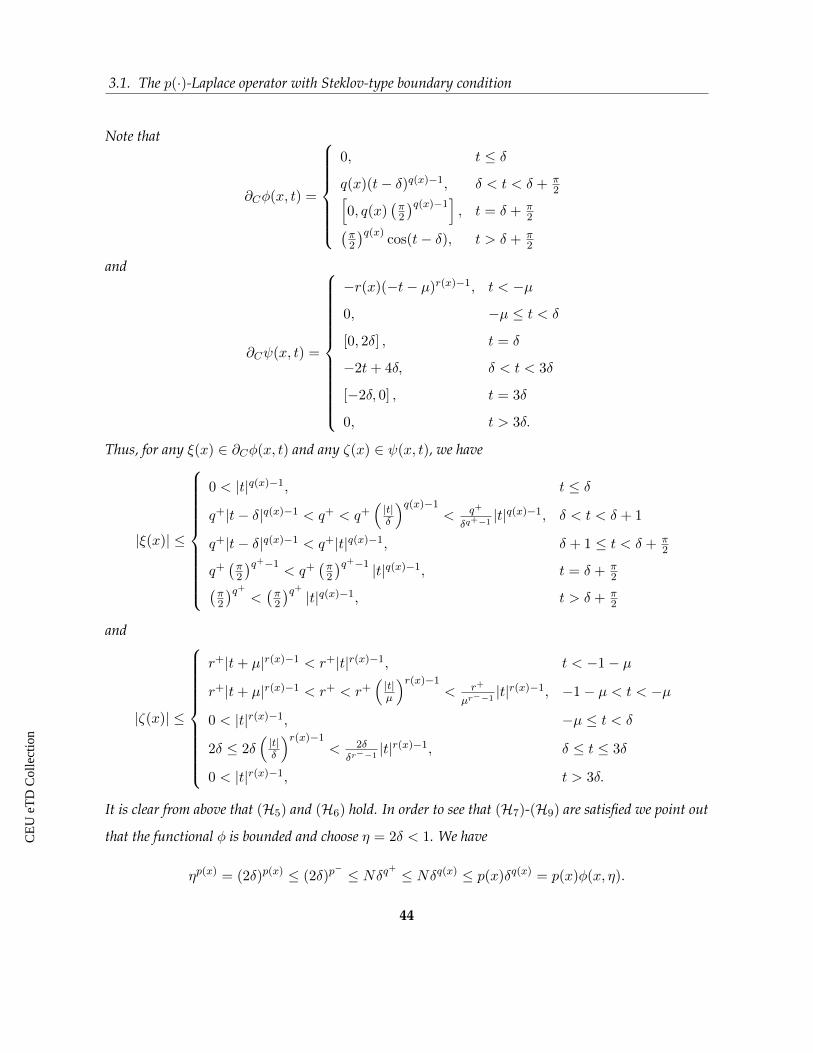
CE
UeT
DC
olle
ctio
n
3.1. The p(·)-Laplace operator with Steklov-type boundary condition
Note that
∂Cφ(x, t) =
0, t ≤ δ
q(x)(t− δ)q(x)−1, δ < t < δ + π2[
0, q(x)(π2
)q(x)−1], t = δ + π
2(π2
)q(x)cos(t− δ), t > δ + π
2
and
∂Cψ(x, t) =
−r(x)(−t− µ)r(x)−1, t < −µ
0, −µ ≤ t < δ
[0, 2δ] , t = δ
−2t+ 4δ, δ < t < 3δ
[−2δ, 0] , t = 3δ
0, t > 3δ.
Thus, for any ξ(x) ∈ ∂Cφ(x, t) and any ζ(x) ∈ ψ(x, t), we have
|ξ(x)| ≤
0 < |t|q(x)−1, t ≤ δ
q+|t− δ|q(x)−1 < q+ < q+(|t|δ
)q(x)−1< q+
δq+−1|t|q(x)−1, δ < t < δ + 1
q+|t− δ|q(x)−1 < q+|t|q(x)−1, δ + 1 ≤ t < δ + π2
q+(π2
)q+−1< q+
(π2
)q+−1 |t|q(x)−1, t = δ + π2(
π2
)q+
<(π2
)q+
|t|q(x)−1, t > δ + π2
and
|ζ(x)| ≤
r+|t+ µ|r(x)−1 < r+|t|r(x)−1, t < −1− µ
r+|t+ µ|r(x)−1 < r+ < r+(|t|µ
)r(x)−1< r+
µr−−1|t|r(x)−1, −1− µ < t < −µ
0 < |t|r(x)−1, −µ ≤ t < δ
2δ ≤ 2δ(|t|δ
)r(x)−1< 2δ
δr−−1|t|r(x)−1, δ ≤ t ≤ 3δ
0 < |t|r(x)−1, t > 3δ.
It is clear from above that (H5) and (H6) hold. In order to see that (H7)-(H9) are satisfied we point out
that the functional φ is bounded and choose η = 2δ < 1. We have
ηp(x) = (2δ)p(x) ≤ (2δ)p− ≤ Nδq+ ≤ Nδq(x) ≤ p(x)δq(x) = p(x)φ(x, η).
44
CE
UeT
DC
olle
ctio
n
3.2. The p-Laplace-like operators with mixed boundary conditions
On the other hand we observe that ψ(x, t) attains its maximum at t = 2δ on [δ, 3δ], ψ(x, 2δ) =
δ2 > 0 and ψ(x, t) = 0 on [−µ, δ] ∪ [3δ, µ], which shows that sup|t|≤µ ψ(x, t) = ψ(x, η), while
supt∈R ψ(x, t) =∞.
We close this section by pointing out the fact that the nonsmooth Ricceri-type multiplic-
ity results presented in Chapter 2 can be successfully applied to other kind of problems. An
example is the following ordinary differential inclusion with periodic boundary conditions
(ODI) :
−u′′ + u ∈ λα(t)∂CF (u) + β(t)∂CG(u) in [0, 1]
u(0) = u(1)
u′(0) = u′(1)
where λ > 0 is a real parameter, F,G : R → R are locally Lipschitz and α, β : [0, 1] → [0,∞)
are nonconstant functions. It can be proved that, under suitable assumptions, for each λ > 0
problem (ODI) has at least two nonzero solutions and there exists λ∗ > 0 for which problem
(ODI) has at least three nonzero solutions. Problems of this type have been insvetigated by F.
Faraci and A. Iannizzotto [48].
Another example is the following differential inclusion on the whole space RN
(Pλ) :
−∆pu+ |u|p−2u ∈ λα(x)∂CF (u(x)) + β(x)∂CG(u(x)) in RN ,
u(x)→ 0 as |x| → ∞,
where λ is a positive real parameter, α, β : RN → R are given and F,G : R → R are two
locally Lipschitz functionals. A similar problem was studied by A. Kristály, W. Marzantowicz
and Cs. Varga [66] using the principle of symmetric criticality. We point out the fact that slightly
modifying the conditions imposed in [66] we can apply Theorem 2.1 to obtain two (or even
three) nonzero solutions for problem (Pλ).
3.2 The p-Laplace-like operators with mixed boundary conditions
Let Ω be a bounded open subset of RN (N ≥ 3) having smooth boundary and 2 ≤ p < +∞. We
denote ∂Ω = Γ the boundary of Ω and assume that Γ1, Γ2 are two open measurable parts that
form a partition of Γ (i.e. Γ1 ∪ Γ2 = Γ and Γ1 ∩ Γ2 = ∅) such that meas(Γ2) > 0.
45
CE
UeT
DC
olle
ctio
n
3.2. The p-Laplace-like operators with mixed boundary conditions
We are interested in boundary value problems involving a quasilinear elliptic differential
operator, a nonsmooth potential and mixed boundary conditions of the following type:
(P2) :
div(a(x,∇u)) ∈ λ∂CF (x, u)− h(x), in Ω
−a(x,∇u) · n ∈ µ(x, u)∂CG(x, u), on Γ1,
u = 0, on Γ2,
where a : Ω× RN → RN is of the form a(x, ξ) = (a1(x, ξ), . . . , aN (x, ξ)), with ai : Ω× RN → R
for i ∈ 1, . . . , N, λ > 0 is a real parameter, F : Ω × R → R and G : Γ1 × R → R are locally
Lipschitz functionals with respect to the second variable, µ : Γ1 × R → R and h : Ω → R
can be viewed as perturbation functions and n is the unit outward normal to ∂Ω. Here and
hereafter, the symbols ∂CF (x, t) and ∂CG(x, t) stand for the Clarke generalized gradients of
the mappings t 7→ F (x, t) and t 7→ G(x, t), respectively.
Example 3.2. Set a(x, ξ) = |ξ|p−2ξ. Then a(x, ξ) is the continuous derivative with respect to the
second variable of the mapping A(x, ξ) = 1p |ξ|
p, i.e. a(x, ξ) = ∇ξA(x, ξ). Then we get the p−Laplace
operator
div(|∇u|p−2∇u).
Example 3.3. Set a(x, ξ) = (1 + |ξ|2)(p−2)/2ξ. Then a(x, ξ) is the continuous derivative with respect
to the second variable of the mapping A(x, ξ) = 1p
[(1 + |ξ|2)p/2 − 1
], i.e. a(x, ξ) = ∇ξA(x, ξ). Then
we get the the mean curvature operator
div(
(1 + |∇u|2)(p−2)/2∇u).
We point out the fact that our operator is not necessarily a potential operator, but we have
chosen these examples due to the fact that boundary value problems involving the above men-
tioned operators were studied intensively in the last decades since quasilinear operators can
model a variety of physical phenomena (e.g. the p-Laplacian is used in non-Newtonian fluids,
reaction-diffusion problems as well as in flow through porous media).
Let us turn now our attention towards the terms given by Clarke’s generalized gradient. To
our best knowledge differential inclusions similar to (P2) have been studied in the past either
46
CE
UeT
DC
olle
ctio
n
3.2. The p-Laplace-like operators with mixed boundary conditions
with Neumann condition, or with Dirichlet condition on the entire boundary. This cases can be
obtained when Γ1 = Γ, or Γ2 = Γ. We present next several particular cases of our problem that
have been treated in the last years by various authors.
CASE 1. Γ1 = Γ (Neumann problem).
• If F and G are primitives of some Carathéodory functions f : Ω × R → R and g :
∂Ω× R→ R
F (x, t) =
∫ t
0f(x, s) ds and G(x, t) =
∫ t
0g(x, s) ds
then the functions t 7→ F (x, t) and t 7→ G(x, t) are differentiable. Thus ∂CF (x, t) =
f(x, t), ∂CG(x, t) = g(x, t) and (P2) reduces to the following eigenvalue prob-
lem div(a(x,∇u)) = λf(x, u)− h(x) in Ω
−a(x,∇u) · n = µ(x, u)g(x, u) on ∂Ω(3.8)
A particular case of problem (3.8) was studied by Y.X. Huang [59] (there the author
studies the case when a(x, ξ) = |ξ|p−2ξ, f(x, t) = m(x)|t|p−2t, g ≡ 0 and h ≡ 0).
• In the case when the functionals f and g from the previous example are only locally
bounded, i.e. f ∈ L∞loc(Ω×R) and g ∈ L∞loc(∂Ω×R) then t 7→ F (x, t) and t 7→ G(x, t)
are locally Lipschitz functionals and, according to Proposition 1.7 in [90] we have
∂CF (x, t) =[f(x, t), f(x, t)
]and ∂CG(x, t) =
[g(x, t), g(x, t)
],
where
f(x, t) = limδ↓0
ess inf|s−t|<δ
f(x, s) f(x, t) = limδ↓0
ess sup|s−t|<δ
f(x, s)
and
g(x, t) = limδ↓0
ess inf|s−t|<δ
g(x, s) g(x, t) = limδ↓0
ess sup|s−t|<δ
g(x, s).
In this case problem (P2) reduces to div(a(x,∇u)) ∈ λ[f(x, u), f(x, u)
]− h(x) in Ω
−a(x,∇u) · n ∈ µ(x, u)[g(x, u), g(x, u)
]on ∂Ω
(3.9)
47
CE
UeT
DC
olle
ctio
n
3.2. The p-Laplace-like operators with mixed boundary conditions
A particular case of problem (3.9) was studied by F. Papalini [102] in the case of
the p-Laplacian. The approach is variational and is based on the nonsmooth critical
point theory for locally Lipschitz functionals developed by K.-C. Chang in [21].
• In the case when h ≡ 0 and µ(x, t) ≡ µ > 0 problem (P2) becomes div(a(x,∇u)) ∈ λ∂CF (x, u), in Ω
−a(x,∇u) · n ∈ µ∂CG(x, u), on ∂Ω,(3.10)
A problem similar to (3.10) was studied by A. Kristály, W. Marzantowicz and Cs.
Varga in [66] where the authors use a nonsmooth three critical points theorem to
prove that there exists a compact interval [a, b] with the property that for every λ ∈
[a, b] there exists µ0 ∈ (0, λ + 1) such the for each µ ∈ [0, µ0], the studied problem
possesses at least three distinct solutions.
CASE 2. Γ2 = Γ (Dirichlet problem).
In this case our problem can be rewritten equivalently as follows:
u ∈W 1,p0 (Ω) : Au+ λ∂CF (·, u) 3 h in W−1,p′(Ω), (3.11)
where Au(x) = −div a(x,∇u(x)).
Problem (3.11) was treated in the case λ = 1 and h ≡ 0 by S. Carl and D. Motreanu [20]
who used the method of sub and supersolutions to obtain general comparison results. We
also remember the work of Z. Liu and G. Liu [75] and J. Wang [121] who studied eigen-
value problems for elliptic hemivariational inequalities that can be rewritten equivalently
as differential inclusions similar to (3.11). In [75] and [121] the authors used the surjectiv-
ity of multivalued pseudomonotone operators to prove the existence of solutions.
As we have seen above, in most papers dealing with differential inclusions of the type (P2)
nonsmooth critical point theory, or the pseudomonotonicity of a certain multivalued operator
play an essential role in obtaining the existence of solutions. However, in all the works we
48
CE
UeT
DC
olle
ctio
n
3.2. The p-Laplace-like operators with mixed boundary conditions
are aware of, additional assumptions on the structure of the elliptic operator and/or the gen-
eralized Clarke’s gradient are needed to obtain the existence of the solution (e.g. the elliptic
operator is of potential type, or the locally Lipschitz functional is required to be regular, or
to satisfy some conditions of Landesman-Lazer type, or the Clarke’s generalized gradient is
supposed to satisfy more restrictive growth conditions). Here, our approach is topological and
the novelty is that we are able to obtain the existence of at least one weak solution for any
λ ∈ (0,+∞) without assuming any of the above restrictions.
We present next the conditions that need to be imposed in order to prove the main result of
this section.
(H10) Let a : Ω × RN → RN be an operator of the form a(x, ξ) = (a1(x, ξ), . . . , aN (x, ξ)) which
satisfies
(i) for each i ∈ 1, . . . , N ai : Ω× RN → R is a Carathéodory function and there exists c0 > 0
and α ∈ Lp′(Ω) such that
|ai(x, ξ)| ≤ α(x) + c0|ξ|p−1,
for a.e. x ∈ Ω and all ξ ∈ RN ;
(ii) there exist c1 > 0 and β ∈ L1(Ω) such that
a(x, ξ) · ξ ≥ c1|ξ|p − β(x),
for a.e. x ∈ Ω and all ξ ∈ RN ;
(iii) for a.e. x ∈ Ω and all ξ1, ξ2 ∈ RN
[a(x, ξ1)− a(x, ξ2)] · (ξ1 − ξ2) ≥ 0.
(H11) Let F : Ω× R→ R be a function which satisfies:
(i) for all t ∈ R the function x 7→ F (x, t) is measurable;
(ii) for a.e. x ∈ Ω the function t 7→ F (x, t) is locally Lipschitz;
49
CE
UeT
DC
olle
ctio
n
3.2. The p-Laplace-like operators with mixed boundary conditions
(iii) there exists c2 > 0 such that for a.e. x ∈ Ω and all t ∈ R
|∂CF (x, t)| ≤ c2(1 + |t|p−1);
(iv) there exists γ1 ∈ Lp(Ω) such that for a.e. x ∈ Ω and all t ∈ R
|F 0(x, t;−t)| ≤ γ1(x)|t|p−1.
(H12) Let G : Γ1 × R → R be measurable with respect to the first variable and assume there
exists γ2 ∈ Lp′(Γ1) such that
|G(x, t1)−G(x, t2)| ≤ γ2(x)|t1 − t2|,
for a.e. x ∈ Γ1 and all t1, t2 ∈ R.
(H13) µ : Γ1 × R→ R is a Carathéodory function and there exists µ∗ > 0 such that
0 ≤ µ(x, t) ≤ µ∗,
for a.e. x ∈ Γ1 and all t ∈ R.
(H14) h ∈ Lp′(Ω).
Let us introduce the functional space
V =v ∈W 1,p(Ω) : γv = 0 on Γ2
where γ : W 1,p(Ω) → Lp(Γ) is the Sobolev trace operator. For simplicity, everywhere below,
we will omit to write γv to indicate the Sobolev trace on the boundary, writing v instead of
γv. Since meas(Γ2) > 0, it is well known that V is a closed subspace of W 1,p(Ω) and can be
endowed with the norm
‖v‖V = ‖∇v‖Lp(Ω),
which is equivalent to the usual norm on W 1,p(Ω) due to the Poincaré-Friedrichs inequality
(see e.g. Proposition 2.94 in [19]).
50
CE
UeT
DC
olle
ctio
n
3.2. The p-Laplace-like operators with mixed boundary conditions
Definition 3.2. We say that u ∈ V is a weak solution for problem (P2) if there exist ζ1 ∈ Lp′(Ω)
satisfying ζ1(x) ∈ ∂CF (x, u(x)) for a.e. x ∈ Ω and ζ2 ∈ Lp′(Γ1) satisfying ζ2(x) ∈ ∂CG(x, u(x)) for
a.e. x ∈ Γ1 such that∫Ωa(x,∇u) · (∇v −∇u) dx+ λ
∫Ωζ1(v − u) dx+
∫Γ1
µ(x, u)ζ2(v − u) dσ =
∫Ωh(x)(v − u) dx,
for all v ∈ V .
The main result of this section is the following theorem.
Theorem 3.2. (N.C., I. FIROIU & F.D. PREDA [27]) Suppose that conditions (H10) − (H14) are
fulfilled. Then for each λ ∈ (0,+∞) problem (P2) possesses at least one weak solution.
Before proving Theorem 3.2 we introduce the operator A : V → V ∗ defined by
〈Au, v〉 =
∫Ωa(x,∇u) · ∇v dx, (3.12)
and denote by φ the element of V ∗ given by
〈φ, v〉 =
∫Ωh(x)v dx.
We have the following proposition which characterizes the weak solutions of problem (P2).
Proposition 3.1. An element u ∈ V is a weak solution for problem (P2) if and only if it solves the
following hemivariational inequality
(HI)λ Find u ∈ V such that
〈Au, v − u〉+ λ
∫ΩF 0(x, u; v − u) dx+
∫Γ1
µ(x, u)G0(x, u; v − u) dσ ≥ 〈φ, v − u〉,
for all v ∈ V .
Finally, we point out the fact that we do not deal with a classical hemivariational inequality
due to the presence of the term∫
Γ1µ(x, u)G0(x, u; v−u) dσ in the left-hand side of the inequality
and consequently several difficulties occur in determining the existence of solutions since the
classical methods fail to be applied directly.
51
CE
UeT
DC
olle
ctio
n
3.2. The p-Laplace-like operators with mixed boundary conditions
Proof of Theorem 3.2. First we point out the fact that under (H10) the operator A : V → V ∗
defined in (3.12) is well defined and satisfies the following properties:
• there exists c3 > 0 such that 〈Au, u〉 ≥ c1‖u‖pV − c3, for all u ∈ V ;
• 〈Av −Au, v − u〉 ≥ 0 for all u, v ∈ V ;
• 〈Aum, v〉 → 〈Au, v〉 for all v ∈ V , whenever um → u in V .
Let us fix λ > 0. We shall prove next that there exists at least one u ∈ V which solves (HI)λ. In
order to do this let us fix R > 0 and define K = BV (0, R) = u ∈ V : ‖u‖V ≤ R and
P =
(v, u) ∈ K ×K 〈Au, v − u〉+ λ∫
Ω F0(x, u; v − u) dx+∫
Γ1µ(x, u)G0(x, u; v − u) dσ ≥ 〈φ, v − u〉
.
After some computations we are able to show that:
For each v ∈ K the set Λ(v) = u ∈ K : (v, u) ∈ P is weakly closed;
For each u ∈ K the set Θ(u) = v ∈ K : (v, u) 6∈ P is either empty or convex;
The set B = u ∈ K : (v, u) ∈ P for all v ∈ K is weakly compact.
The above statements show that we can apply Lin’s theorem (see [73], Theorem ), for the weak
topology of the space V , with K0 = K = BV (0,m) and obtain the existence of an element
um ∈ BV (0,m) such that BV (0,m)× um ⊆ P , which can be rewritten equivalently as
〈Aum, v − um〉+ λ
∫ΩF 0(x, um, v − um) dx+
∫Γ1
G0(x, um; v − um) dσ ≥ 〈φ, v − um〉, (3.13)
for all v ∈ BV (0,m), which means that, for each positive integer m, the restriction of (HI)λ to
BV (0,m) possesses at least one solution.
In order to compete the proof we need to prove that there exists m∗ > 0 such that
um∗ ∈ BV (0,m∗) (3.14)
and this um∗ solves (HI)λ. This can be easily done as follows.
52
CE
UeT
DC
olle
ctio
n
3.2. The p-Laplace-like operators with mixed boundary conditions
Arguing by contradiction let us assume that ‖um‖V = m for all m > 0. Taking v = 0 in
(3.13) we obtain
〈Aum, um〉 ≤ 〈φ, um〉+ λ
∫ΩF 0(x, um;−um) dx+
∫Γ1
µ(x, um)G0(x, um;−um) dσ
≤ ‖φ‖V ∗‖um‖V + λ
∫Ωγ1(x)|um|p−1 dx+ µ∗
∫Γ1
γ2(x)|um| dσ
≤ ‖φ‖V ∗‖um‖V + λ‖γ1‖Lp(Ω)‖um‖p−1Lp(Ω) + µ∗‖γ2‖Lp′ (Γ1)‖um‖Lp(Γ1)
≤ c1‖um‖V + c2‖um‖p−1V ,
for some suitable constants c1, c2 > 0. On the other hand, we know that
〈Aum, um〉 ≥ c1‖um‖pV − c3.
Combining the above estimates and keeping in mind that 1 < p and ‖um‖V = m for all m > 0
we arrive at
c1mp − c3 ≤ c1m
p−1 + c2m.
Dividing by mp−1 and letting m → ∞ we get a contradiction as the left-hand term of the
inequality diverges while the right-hand term remains bounded, which is impossible. This
contradiction shows that (3.14) holds.
Now let v ∈ V be fixed. We know that ‖um∗‖V < m∗ which allows us to choose t ∈ (0, 1)
such that w = um∗ + t(v − um∗) ∈ BV (0,m∗). Plugging w in (3.13) we have
t〈φ, v − um∗〉 = 〈φ,w − um∗〉
≤ 〈Aum∗ , w − um∗〉+ λ
∫ΩF 0(x, um∗ ;w − um∗) dx+∫
Γ1
µ(x, um∗)G0(x, um∗ ;w − um∗) dσ
= t
[〈Aum∗ , v − um∗〉+ λ
∫ΩF 0(x, um∗ ; v − um∗) dx +∫
Γ1
µ(x, um∗)G0(x, um∗ ; v − um∗) dσ
].
Dividing the above relation by t > 0 we conclude that um∗ is indeed a solution for (HI)λ.
53
CE
UeT
DC
olle
ctio
n
3.3. The p(·)-Laplace operator with the Dirichlet boundary condition
3.3 The−→p (·)-Laplace operator with the Dirichlet boundary condition
In this section we study the weak solvability of a differential inclusion involving a nonhomo-
geneous anisotropic differential operator of the following type
(P3) :
−
n∑i=1
∂i(|∂iu|pi(x)−2∂iu
)∈ λ∂Cα(x, u) + ∂Cβ(x, u) in Ω,
u = 0 on ∂Ω,
where Ω ⊂ Rn (n ≥ 3) is a bounded open set with smooth boundary, λ > 0 is a real parameter,
α, β : Ω×R→ R are two locally Lipschitz functions with respect to the second variable and, for
each i ∈ 1, . . . , n, pi : Ω → R is a continuous function such that 2 ≤ pi(x) < n for all x ∈ Ω.
The notation ∂iu stands for the partial derivative of u with respect to the xi component, that
is ∂u/∂xi, while ∂Cα(x, t) denotes the Clarke generalized gradient of the function t 7→ α(x, t).
The definition and main properties of the Clarke generalized gradient will be given in the next
section.
We point out the fact that, if α(x, t) = 1q(x) |t|
q(x) and β ≡ const., then problem (P3) reduces
to the following nonhomogeneous anisotropic eigenvalue problem−
n∑i=1
∂i(|∂iu|pi(x)−2∂iu
)= λ|u|q(x)−2u in Ω,
u = 0 on ∂Ω,
(3.15)
which was studied by Mihailescu, Pucci and Radulescu [84, 85]. In these papers the authors
show that the “competition” between the growth rates of the functions pi and q deeply influ-
ence the existence or nonexistence of the weak solutions. To our best knowledge these are the
first papers dealing with the anisotropic variable exponent −→p (·)-Laplace operator, i.e.
∆−→p (·)u =
n∑i=1
∂i
(|∂iu|pi(x)−2∂iu
),
where−→p : Ω→ Rn is the vectorial function−→p (·) = (p1(·), . . . , pn(·)). Also in these papers it was
introduced for the first time the anisotropic exponent Sobolev space W 1,−→p (·)0 (Ω) that allowed
an accurate study of problems of the type (3.15). We point out that the aforementioned space
can be viewed as a natural generalization of the variable exponent Sobolev space W 1,p(·)0 (Ω)
54
CE
UeT
DC
olle
ctio
n
3.3. The p(·)-Laplace operator with the Dirichlet boundary condition
(when p1(·) = · · · = pn(·) = p(·)) as well as a natural generalization of the classical anisotropic
Sobolev space W 1,−→p0 (Ω) (when pi are constant functions, i ∈ 1, . . . , n).
On the other hand, let us consider the case when α ≡ const. and β is the primitive of some
Carathéodory function f : Ω× R→ R
β(x, t) =
t∫0
f(x, s) ds.
Then the function t 7→ β(x, t) is differentiable and thus ∂Cβ(x, t) = f(x, t) and problem (P3)
reduces to the following nonhomogeneous anisotropic problem−
n∑i=1
∂i(|∂iu|pi(x)−2∂iu
)= f(x, u) in Ω,
u = 0 on ∂Ω,
(3.16)
which was studied recently by Boureanu, Pucci and Radulescu [12], by using the symmetric
mountain-pass theorem of Ambrosetti and Rabinowitz.
The abstract framework required to study differential inclusions of the type (P3) lies at the
interface of three important directions in analysis:
• the nonsmooth analysis: the need for such theory comes naturally whenever we deal with
functions which are not differentiable everywhere, but are convex or locally Lipschitz
(see, e.g., Andrei, Costea and Matei [4], Chang [21], Clake [24], Costea and Varga [37, 38],
Kristály, Radulescu and Varga [67], Motreanu and Panagiotopoulos [90], Motreanu and
Radulescu [91], Naniewicz and Panagiotopoulos [94], Panagiotopoulos [98, 99, 100]).
• the variable exponent Lebesgue-Sobolev spaces theory: problems involving the isotropic p(x)-
Laplace operator have captured special attention in the last decades since they can model
various phenomena which arise in elastic mechanics (see, e.g., Zhikov [123]), image restora-
tion (see, e.g., Chen, Levine and Rao [23]) or electrorheological fluids (see, e.g., Acerbi and
Mingione [1], Diening [42], Diening, Harjulehto, Hästö and Ružicka [43], Halsey [55],
Ružicka [109], Costea and Mihailescu [33], Mihailescu and Radulescu [86, 87]).
55
CE
UeT
DC
olle
ctio
n
3.3. The p(·)-Laplace operator with the Dirichlet boundary condition
• the anisotropic Sobolev spaces theory: the need for such theory comes naturally whenever we
deal with materials possessing inhomogeneities that have different behavior on different
space directions (see, e.g., Edmunds and Edmunds [44], Nikol’skii [97], Rákosník [104,
105], Troisi [119]).
Although the −→p (·)-Laplace operator was introduced recently, in 2007 by Mihailescu, Rad-
ulescu and Pucci, problems involving this operator, or similar operators, have captured special
attention in the last years (see Boureanu, Pucci and Radulescu [12], Fan [45], Mihailescu and
Morosanu [81], Mihailescu, Morosanu and Radulescu [82, 83], Stancu-Dumitru [117]). How-
ever, in all the works we are aware of, the energy functional attached to the problem is smooth,
while differential inclusions like problem (P3), for which the attached energy functional is only
locally Lipschitz and not differentiable, have not yet been studied.
In this section we prove a multiplicity result concerning the weak solutions of problem
(P3). Before defining the concept of weak solution we denote by X the anisotropic variable
exponent Sobolev space W 1,−→p (·)0 (Ω) and by ‖ · ‖ the norm defined on this space, that is ‖ · ‖−→p (·).
Definition 3.3. A function u ∈ X is called a weak solution for problem (P3) if, for a.e. x ∈ Ω, there
exist ξ(x) ∈ ∂Cα(x, u(x)) and ζ(x) ∈ ∂Cβ(x, u(x)) such that∫Ω
n∑i=1
|∂iu|pi(x)−2∂iu∂iv dx = λ
∫Ωξv dx+
∫Ωζv dx, for all v ∈ X.
In order to obtain our main result we shall assume fulfilled the following hypotheses.
(H15) For each i ∈ 1, . . . , n the function pi ∈ C+(Ω) is log-Hölder continuous, 2 ≤ pi(x) < n
for all x ∈ Ω and p+M < P ∗;
(H16) The function α : Ω× R→ R satisfies
(i) α(x, 0) = 0 for a.e. x ∈ Ω;
(ii) x 7→ α(x, t) is measurable for all t ∈ R;
(iii) t 7→ α(x, t) is locally Lipschitz for a.e. x ∈ Ω;
56
CE
UeT
DC
olle
ctio
n
3.3. The p(·)-Laplace operator with the Dirichlet boundary condition
(iv) there exist cα > 0 and q ∈ C+(Ω) such that 1 < q− ≤ q+ < p−m and
|ξ(x)| ≤ cα|t|q(x)−1
for a.e. x ∈ Ω, all t ∈ R and all ξ(x) ∈ ∂Cα(x, t);
(v) there exist µ ∈ (0, 1), α0 > 0 and t0 > 0 such that
α(x, t) ≤ 0, for all |t| < µ and a.e. x ∈ Ω,
and
α(x, t0) ≥ α0 > 0, for a.e. x ∈ Ω.
(H17): The function β : Ω× R→ R satisfies
(i) β(x, 0) = 0 for a.e. x ∈ Ω;
(ii) x 7→ β(x, t) is measurable for all t ∈ R;
(iii) there exists r ∈ C+(Ω) with the property that 1 < r(x) < P ∗ and K ∈ Lr′(·)(Ω) such
that
|β(x, t1)− β(x, t2)| ≤ K(x)|t1 − t2|
for a.e. x ∈ Ω and all t1, t2 ∈ R;
(iv) β(x, t) ≤ 0, for a.e. x ∈ Ω and all t ∈ R.
The main result of this section is given by the following theorem.
Theorem 3.3. (N.C. & G. MOROSANU [31]) Assume that (H15), (H16) and (H17) hold. Then there
exists λ∗ > 0 such that for any λ ∈ (λ∗,+∞) problem (P3) possesses at least two non-zero weak
solutions.
Proof. Let us introduce the functionals J : X → R, Λ : Lq(·)(Ω) → R and Θ : Lr(·)(Ω) → R
defined by
J(u) :=
∫Ω
n∑i=1
|∂iu|pi(x)
pi(x)dx, Λ(w) :=
∫Ωα(x,w(x)) dx, Θ(z) :=
∫Ωβ(x, z(x)) dx.
57
CE
UeT
DC
olle
ctio
n
3.3. The p(·)-Laplace operator with the Dirichlet boundary condition
Standard arguments can be employed in order to conclude that the functional Eλ : X → R
defined by
Eλ(u) = J(u)−Θ(u)− λΛ(u),
is locally Lipschitz and each critical point of this functional is a solution of problem (P3). More-
over, it can be shown that Eλ is sequentially weakly lower semicontinuous, coercive and satis-
fies the (PS)-condition. The following claims complete the proof.
CLAIM 1. There exists λ∗ > 0 such that for any λ > λ∗ we can determine u0 ∈ X for which
Eλ(u0) < 0.
Let x0 ∈ int Ω be such that the distance from x0 to the boundary of Ω is maximal and
let R0 be this distance (R0 = maxx∈Ω
miny∈∂Ω
|x − y|). Clearly, for 0 < R < R0/2, we have
B(x0; 2R) ⊆ Ω. It can be easily seen that there exists u0 ∈ C∞0 (B(x0; 2R)) such that u0(x) = t0 for x ∈ B(x0;R)
0 ≤ u0(x) ≤ t0 for x ∈ B(x0; 2R) \B(x0;R).
Since u0 ∈ C∞0 (B(x0; 2R)), for i ∈ 1, . . . , n, there exists mi > 0 such that |∂iu0(x)| ≤ mi
in B(x0; 2R). Then for m := max1,m1 . . . ,mnwe have
Eλ(u0) =
∫Ω
n∑i=1
|∂iu0(x)|pi(x)
pi(x)dx−
∫Ωβ(x, u0(x)) dx− λ
∫Ωα(x, u0(x)) dx
≤∫B(x0;2R)
n∑i=1
mp+M
p−mdx−
∫B(x0;2R)
β(x, u0(x)) dx− λ∫B(x0;2R)
α(x, u0(x)) dx.
Obviously,
−∫B(x0;2R)
β(x, u0(x)) dx =
∫B(x0;2R)
β(x, 0)− β(x, u0(x)) dx
≤∫B(x0;2R)
K(x)u0(x) dx ≤ β1,
for a suitable constant β1 > 0.
On the other hand, splitting B(x0; 2R) into the sets
D1 = x ∈ B(x0; 2R) : α(x, u0(x)) ≤ 0
58
CE
UeT
DC
olle
ctio
n
3.3. The p(·)-Laplace operator with the Dirichlet boundary condition
and
D2 = x ∈ B(x0; 2R) : α(x, u0(x)) > 0 ,
we observe thatB(x0;R) ⊂ D2. Applying Lebourg’s mean value theorem and taking into
account hypothesis (H16) one can easily prove that∫B(x0;2R)
α(x, u0(x)) dx ≥ −α1 + α0ωnR
n
n,
where ωn is the area of the unit sphere in Rn and α1 > 0 is a suitable constant.
Thus
Eλ(u0) ≤ mp+M 2nωnR
n
p−m+ β1 + α1 − λα0
ωnRn
n< 0,
for any λ > n2nmp+M ωnRn+n(β1+α1)p−m
α0ωnRn.
CLAIM 2. The functional Eλ possesses two critical points u1, u2 ∈ X \ 0, provided that
λ ∈ (λ∗,+∞).
The facts that Eλ is sequentially lower semicontinuous and coercive allow us to apply
Theorem 1.2 to obtain the existence of an element u1 ∈ X such that Eλ(u1) = minu∈XEλ(u).
Obviously u1 is a critical point of Eλ as it is a global minimizer, while CLAIM 1 ensures
that Eλ(u1) < 0, which means that u1 6= 0. Furthermore, if there exists ρ ∈ (0, ‖u1‖) such
that
inf∂B(0;ρ)
Eλ ≥ 0 = maxEλ(0), Eλ(u1),
then we can apply Theorem 1.3 to obtain another critical point u2 ∈ X \ 0, u1.
Let us consider s ∈ C+(Ω) such that p+M < s− ≤ s+ < P ∗ and choose ρ > 0 such
that ρ < min1, 1/cs, ‖u1‖, where cs > 0 is the constant given by the compact inclusion
W1,−→p (·)0 (Ω) → Ls(·)(Ω), i.e.,
‖u‖s(·) ≤ cs‖u‖, for all u ∈W 1,−→p (·)0 (Ω).
59
CE
UeT
DC
olle
ctio
n
3.3. The p(·)-Laplace operator with the Dirichlet boundary condition
Then for each u ∈ ∂B(0; ρ) we have ‖∂iu‖pi(·) < 1 (1 ≤ i ≤ n) and ‖u‖s(·) < 1. Thus for
u ∈ X such that ‖u‖ = ρ we have
Eλ(u) = J(u)−Θ(u)− λΛ(u)
≥ 1
p+M
n∑i=1
∫Ω|∂iu|pi(x) dx−
∫Ωβ(x, u(x)) dx− λ
∫Ωα(x, u(x)) dx
≥ 1
p+M
n∑i=1
‖∂iu‖p+M
pi(·) − λ∫
Ωα(x, u(x)) dx.
Using the convexity of the function h : R+ → R+ defined by h(t) = tp+M we deduce that
n∑i=1
‖∂iu‖p+M
pi(·) ≥1
np+M−1‖u‖p
+M .
Defining Ω1 = x ∈ Ω : |u(x)| < µ and Ω2 = x ∈ Ω : |u(x)| ≥ µ and by the use of
hypothesis (H16)− (v) and Lebourg’s mean value theorem we can prove that∫Ωα(x, u(x)) dx ≤ cµq+−s−‖u‖s−s(·) ≤ cµ
q+−s−cs−s ‖u‖s
−,
for a suitable constant c > 0.
Thus, for u ∈ ∂B(0; ρ)
Eλ(u) ≥ 1
p+Mn
p+M−1
ρp+M − λcµq+−s−cs
−s ρs
−= ρp
+M
(1
p+Mn
p+M−1
− λcµq+−s−cs−s ρs
−−p+M
).
Finally, we observe that the function h : [0, 1]→ R defined by
h(t) =1
p+Mn
p+M−1
− λcµq+−s−cs−s ts
−−p+M
is continuous on [0, 1] and h(0) = 1
p+Mn
p+M−1
> 0, hence h > 0 in a small neighborhood
at the right of the origin. Choosing ρ > 0 such that ρ belongs to this neighborhood and
ρ < min1, 1/cs, ‖u1‖ we deduce that Eλ(u) > 0 for all u ∈ ∂B(0; ρ) and this completes
the proof.
60
CE
UeT
DC
olle
ctio
n
3.3. The p(·)-Laplace operator with the Dirichlet boundary condition
We close this section with several examples of functions α, β : Ω× R→ R for which condi-
tions (H16) and (H17) are fulfilled.
Example 3.4. Let εk be a sequence of positive real numbers such that εk ↓ 0 as k → +∞. Let
q ∈ C+(Ω) be such that 1 < q− ≤ q+ < p−m and let αk, βk : Ω× R→ R to be defined by
αk(x, t) =
1
q(x) |t+ εk|q(x), for t ∈ (−∞,−εk],
0, for t ∈ (−εk, εk),1
q(x) |t− εk|q(x), for t ∈ [εk,+∞),
and
βk(x, t) = 0, for all (x, t) ∈ Ω× R.
Then, ∂Cβ(x, t) = 0 for all (x, t) ∈ Ω× R, while
∂Cαk(x, t) =
|t+ εk|q(x)−2(t+ εk), for t ∈ (−∞,−εk),
0, for t ∈ [−εk, εk],
|t− εk|q(x)−2(t− εk), for t ∈ (εk,+∞).
Thus, for any ξ(x) ∈ ∂Cα(x, t), we have
|ξ(x)| ≤
|t|q(x)−1 ≤ 1
εq+−1k
|t|q(x)−1, for |t| ∈ [1 + εk,+∞),
1 ≤(|t|εk
)q(x)−1≤ 1
εq+−1k
|t|q(x)−1, for |t| ∈ (εk, 1 + εk),
0 ≤ 1
εq+−1k
|t|q(x)−1, for |t| ∈ [0, εk).
We point out the fact that when k → +∞ then problem (P3) with αk, βk defined above reduces to
problem (3.15), hence this example shows that slightly perturbing problem (3.15) around the origin we
can obtain two nontrivial weak solutions instead of only one weak solution as Theorem 3 [85] states.
Example 3.5. Let µ ∈ (0, 1), q1, q2 ∈ C+(Ω) be such that 1 < q−1 ≤ q+1 < q−2 ≤ q+
2 < p−m and let
a ∈ L∞(Ω) be such that a(x) < 0 for a.e. x ∈ Ω. We consider the functions α, β : Ω × R → R to be
defined by
α(x, t) =
0, for t ∈ (−∞, µ),
max
(t− µ)q1(x), (t− µ)q2(x), for t ∈ [µ,+∞),
61
CE
UeT
DC
olle
ctio
n
3.3. The p(·)-Laplace operator with the Dirichlet boundary condition
and
β(x, t) = a(x)|t|.
Then
∂Cα(x, t) =
0, for t ∈ (∞, µ],
q1(x)(t− µ)q1(x)−1, for t ∈ (µ, 1 + µ),
[q1(x), q2(x)] , for t = 1 + µ,
q2(x)(t− µ)q2(x)−1, for t ∈ (1 + µ,+∞),
and
∂Cβ(x, t) =
−a(x), for t ∈ (−∞, 0),
[a(x),−a(x)] , for t = 0,
a(x), for t ∈ (0,+∞).
Thus for every ξ(x) ∈ ∂Cα(x, t) we have
|ξ(x)| ≤
0 ≤ q+2
µq+2 −1|t|q2(x)−1, for t ∈ (−∞, µ],
q+1 ≤ q
+2
(|t|µ
)q2(x)−1≤ q+
2
µq+2 −1|t|q2(x)−1, for t ∈ (µ, 1 + µ),
q+2 ≤
q+2
µq+2 −1|t|q2(x)−1, for t = 1 + µ,
q+2 |t− µ|q2(x)−1 ≤ q+
2
µq+2 −1|t|q2(x)−1, for t ∈ [1 + µ,+∞).
Example 3.6. Let f, g ∈ L∞loc(Ω× R) and consider α, β : Ω× R be defined by
α(x, t) =
∫ t
0f(x, s) ds and β(x, t) =
∫ t
0g(x, s) ds.
Obviously, t 7→ α(x, t) and t 7→ β(x, t) are locally Lipschitz and according to Proposition 1.7 in
Motreanu and Panagiotopoulos [90], we have
∂Cα(x, t) =[f(x, t), f(x, t)
]and ∂Cβ(x, t) =
[g(x, t), g(x, t)
],
where for a function h ∈ L∞loc(Ω× R) we denote by
h(x, t) = limδ↓0
inf|s−t|<δ
h(x, t) and h(x, t) = limδ↓0
sup|s−t|<δ
h(x, t).
Clearly, there are many ways in which we can choose f and g such that conditions (H16) and (H17) are
fulfilled.
62
CE
UeT
DC
olle
ctio
n
Chapter 4
Differential inclusions in
Orlicz-Sobolev spaces
4.1 Formulation of the problem
In this chapter we establish an existence result for differential inclusions involving quasilinear
elliptic operators in divergence form of the following type
Au := div (a(|∇u|)∇u) , (4.1)
subjected to Dirichlet boundary conditions, in a bounded domain with smooth boundary. More
exactly, we are interested in the existence of weak solutions for the problem
(P) :
−div (a(|∇u|)∇u) ∈ ∂CF (x, u), in Ω,
u = 0, on ∂Ω,
where Ω is a bounded, open subset of RN (N ≥ 2) with smooth boundary ∂Ω and a : [0,∞)→
[0,∞) is a mapping such that the function ϕ : R→ R defined by
ϕ(t) = a(|t|)t,
63
CE
UeT
DC
olle
ctio
n
4.1. Formulation of the problem
is continuous, strictly increasing and onto. Here, F : Ω× R→ R is a locally Lipschitz function
with respect to the second variable and, as usual, ∂CF (x, t) denotes the Clarke generalized
gradient of the mapping t 7→ F (x, t).
As Ruf [108] pointed out, in dealing with variational problems of the type (P) two questions
arise naturally:
(Q1): Which is the appropriate function space for the problem to be well-posed, hence solvable?
(Q2): What kind of growth conditions on F would ensure the existence of weak solutions?
The answer to (Q1) is determined by two competing factors: on the one hand the space should
be "large enough" such that the functional attached to the problem satisfies an appropriate
compactness condition (e.g. Palais-Smale or Cerami condition) which ensures that a sequence
for which the functional converges to a critical value has a convergent subsequence; and, on
the other hand, the space should be "small enough" such that the functional has the desired
regularity (locally Lipschitz in our case). In the classical case of the p-Laplacian, i.e. a(s) = sp−2
and
Au = ∆pu = div(|∇u|p−2∇u
)the suitable space in which the problem is studied is the Sobolev space W 1,p(Ω). However, in
our framework, the space Lp(Ω) needs to be replaced by the Orlicz space LΦ(Ω) in which the
role of the convex function tp is played by the N -function Φ. It is also worth mentioning that
these spaces fill a gap in the Sobolev embedding theorem as, for mp = N ,
Wm,p(Ω) → Lq(Ω), for all q ∈ [p,∞),
but
Wm,p(Ω) 6→ L∞(Ω),
hence there is no smallest Lq space in which Wm,p(Ω) can be embedded. Trudinger [120]
showed that the best target to embed the space Wm,p(Ω) is the Orlicz space LΦ(Ω) with
Φ(t) = exp(|t|p/(p−1)
)− 1.
64
CE
UeT
DC
olle
ctio
n
4.1. Formulation of the problem
Regarding (Q2), it is well known that in the case of the p-Laplacian an important role is
played by the critical exponent in the Sobolev embedding theorem p∗ = Np/(N − p) for which
the space setup works and one is able to prove existence results if subcritical growth assump-
tions are imposed, while in the critical case we may have nonexistence results. For example let
us consider the particular case
a(s) = 1, ∀s ≥ 0 and F (t) =
∫ t
0f(s)ds
with f : R → R a continuous function. Then, F is differentiable and the ∂CF (t) = f(t) and
problem (P) becomes −∆u = f(u), in Ω,
u = 0, on ∂Ω.(4.2)
Clearly, the suitable choice for the function space is H10 (Ω) and if f has "subcritical growth",
that is
|f(t)| ≤ c1 + c2|t|q, 1 < q < 2∗ − 1,
where 2∗ = 2NN−2 , then one can prove the existence of solutions, while in the "critical growth"
case
f(t) = t2∗−1,
one can use Pohozaev’s identity to prove that problem (4.2) has only the trivial solution if Ω is
bounded and starshaped.
In this chapter, we consider the case when ϕ : R → R, ϕ(t) = a(|t|)t, defines an admissible
function and the nonlinearity F has subcritical growth and we will employ variational methods
to prove the existence of at least one weak solution for our problem. Let us start by specifying
what we understand by weak solution for problem (P).
Definition 4.1. A function u ∈ W 10L
Φ(Ω) is called weak solution for problem (P) if, for a.e. x ∈ Ω,
there exists ξ(x) ∈ ∂CF (x, u(x)) such that∫Ωa(|∇u|)∇u · ∇v dx =
∫Ωξv dx, for all v ∈W 1
0LΦ(Ω).
65
CE
UeT
DC
olle
ctio
n
4.2. An existence result
4.2 An existence result
In order to apply the Direct Method in the Calculus of Variations and show that the energy
functional attached to problem (P) has a global minimizer, hence a critical point, we will im-
pose the following hypotheses.
(H0) The functions ϕ,ψ : R→ R are admissible and satisfy
(i) ϕ(t) = a(|t|)t;
(ii) 1 < ϕ− ≤ ϕ+ <∞ and 1 < ψ− ≤ ψ+ <∞;
(iii) The corresponding N -function of ψ, i.e. Ψ(t) =∫ t
0 ψ(s) ds, increases essentially slower
than Φ∗ whenever ∫ ∞1
φ−1(t)
t(N+1)/Ndt =∞.
(HF ) F : Ω× R→ R is a Carathéodory function such that
(i) F (x, 0) = 0 for a.e. x ∈ Ω;
(ii) t 7→ F (x, t) is locally Lipschitz for a.e. x ∈ Ω;
(iii) there exists b ∈ LΨ∗(Ω) such that
|ξ| ≤ b(x) + ψ(|t|),
for a.e. x ∈ Ω, all t ∈ R and all ξ ∈ ∂CF (x, t).
Let us consider the functionals JΦ : W 10L
Φ(Ω)→ R and JF : LΨ(Ω)→ R defined by
JΦ(u) =
∫Ω
Φ(|∇u|) dx,
and
JF (w) =
∫ΩF (x,w(x)) dx.
The energy functional corresponding to problem (P), E : W 10L
Φ(Ω)→ R, is given by
E(u) = JΦ(u)− JF (u). (4.3)
66
CE
UeT
DC
olle
ctio
n
4.2. An existence result
Condition (H0) ensures that W 10L
Φ(Ω) is compactly embedded into LΨ(Ω), hence E is well
defined. The following lemma guarantees the fact that, in order to solve problem (P), it suffices
to seek for critical points, in the sense of Definition 1.10, of the energy functional attached to
our problem.
Lemma 4.1. Assume (H0) and (HF ) hold. Then the functional E : W 10L
Φ(Ω) → R defined in (4.3)
has the following properties:
(i) E is locally Lipschitz;
(ii) E is weakly lower semicontinuous;
(iii) each critical point of E is a weak solution for problem (P1).
Proof. (i) According to Lemma A.6 in [25] JΦ ∈ C1(W 1
0LΦ(Ω),R
)and
〈J ′Φ(u), v〉 =
∫Ωa(|∇u|)∇u · ∇v dx (4.4)
Since W 10L
Φ(Ω) is compactly embedded into LΨ(Ω) there exists c1 > 0 such that
|u|Ψ ≤ c1‖u‖, for all u ∈W 10L
Φ(Ω), (4.5)
with ‖ · ‖ defined as in Section 1.3, that is ‖u‖ = | |∇u| |Φ. Let us fix now u0 ∈ W 10L
Φ(Ω)
and prove that there exists r > 0 sufficiently small such that E is Lipschitz continuous
on BW 10L
Φ(Ω)(u0, r) =v ∈W 1
0LΦ(Ω) : ‖v − u0‖ ≤ r
. Theorem 2.3 ensures the existence
of an r0 > 0 such that JF is Lipschitz continuous on BLΨ(Ω)(u0, r0), hence there exists a
positive constant L such that
|JF (w1)− JF (w2)| ≤ L|w1 − w2|Ψ, for all w1, w2 ∈ BLΨ(Ω)(u0, r0). (4.6)
From (4.5) and (4.6) we get
|JF (u1)− JF (u2)| ≤ Lc1‖u1 − u2‖, for all u1, u2 ∈ BW 10L
Φ(Ω)(u0, r0/c1). (4.7)
67
CE
UeT
DC
olle
ctio
n
4.2. An existence result
On the other hand, for r = r0/c1 and u1, u2 ∈ BW 10L
Φ(Ω)(u0, r) we have
|JΦ(u1)− JΦ(u2)| ≤ |〈J ′Φ(u), u1 − u2〉|
≤ ‖J ′Φ(u)‖[W 10L
Φ(Ω)]∗‖u1 − u2‖,
for some u ∈ λu1 + (1− λ)u2 : λ(0, 1). The space W 10L
Φ(Ω) is reflexive, hence the ball
BW 10L
Φ(Ω)(u0, r) is weakly compact, therefore there exists m > 0 such that
‖J ′Φ(u)‖[W 10L
Φ(Ω)]∗ ≤ m. (4.8)
Taking into account (4.7) and (4.8) we conclude thatE is a Lipschitz continuous functional
on BW 10L
Φ(Ω)(u0, r).
(ii) Let un ⊂W 10L
Φ(Ω) be such that un u in W 10L
Φ(Ω). Reasoning as in Lemma 3.2 in [52]
we infer that JΦ is weakly lower semicontinuous, hence
JΦ(u) ≤ lim infn→∞
JΦ(un).
On the other hand, un → u in LΨ(Ω) and by Fatou’s lemma
lim supn→∞
JF (un) = lim supn→∞
∫ΩF (x, un(x)) dx
≤∫
Ωlim supn→∞
F (x, un(x)) dx
=
∫ΩF (x, u(x)) dx
= JF (u),
which shows that JF is weakly upper semicontinuous on W 10L
Φ(Ω).
(iii) Let u ∈ W 10L
Φ(Ω) be a critical point of E. According to Propositions 2.3.1 and 2.3.2 in
Clarke [24]
0 ∈ ∂CE(u) ⊆ J ′Φ(u)− ∂CJF (u),
hence there exists η ∈ ∂CJF (u) such that
〈J ′Φ(u), v〉 = 〈η, v〉, for all v ∈W 10L
Φ(Ω). (4.9)
68
CE
UeT
DC
olle
ctio
n
4.2. An existence result
Theorem 2.3 ensures the existence of a ξ ∈ LΨ∗(Ω) which satisfies ξ(x) ∈ ∂CF (x, u(x)), for a.e. x ∈ Ω,
〈η, v〉 =∫
Ω ξ(x)v(x) dx, for all v ∈W 10L
Φ(Ω).(4.10)
The conclusion follows at once from (4.4), (4.9) and (4.10).
Theorem 4.1. Suppose (H0) and (HF ) are fulfilled and assume in addition that ψ+ < ϕ−. Then
problem (P) has a nontrivial weak solution.
Proof. The idea is to prove that E is coercive and apply Theorem 1.2 to conclude that E pos-
sesses a global minimum point. To this end, let u ∈W 10L
Φ(Ω) be such that ‖u‖ > 1. Then, from
(2.8), we have
JΦ(u) ≥ | |∇u| |ϕ−
Φ = ‖u‖ϕ− . (4.11)
On the other hand, we can apply Lebourg’s mean value theorem to deduce that there exist
λ0 ∈ (0, 1) and ζ ∈ ∂CF (x, λ0u) such that
F (x, u(x)) = F (x, u(x))− F (x, 0) = ζ(x)u(x), for a.e. x ∈ Ω.
Thus,
JF (u) =
∫ΩF (x, u(x)) dx
≤∫
Ω|ζ||u| dx
≤∫
Ω[b(x) + ψ (λ0|u|)] |u| dx
≤ 2|b|Ψ∗ |u|Ψ +1
λ0
∫Ωλ0|u|ψ(λ0|u|) dx.
Using Young’s inequality we get
λ0|u|ψ(λ0|u|) ≤∫ 2λ0|u|
λ0|u|ψ(s) ds ≤ Ψ(2λ0|u|),
69
CE
UeT
DC
olle
ctio
n
4.2. An existence result
and the ∆2-condition yields∫Ωλ0|u|ψ(λ0|u|) dx ≤
∫Ω
Ψ(2λ0|u|) dx ≤ C1 + C2
∫Ω
Ψ(λ0|u|) dx,
for some suitable positive constants C1 and C2. Clearly, relations (2.8) and (2.9) imply∫Ω
Ψ(λ0|u|) dx ≤ λ0
(|u|ψ
+
Ψ + |u|ψ−
Ψ
).
The above relations together with (4.5) lead to the following estimate
JF (u) ≤ C3 + C4‖u‖+ C5‖u‖ψ−
+ C6‖u‖ψ+, (4.12)
for some suitable positive constants C3, C4, C5, C6. Taking into account (4.11) and (4.12) we
infer that E(u)→∞ as ‖u‖ → ∞.
70
CE
UeT
DC
olle
ctio
n
Chapter 5
Variational-like inequality problems
governed by set-valued operators
In 1989, J. Parida, M. Sahoo and S. Kumar [103] introduced a new type of inequality problem
of variational type which had the form
Find u ∈ K such that
〈A(u), η(v, u)〉 ≥ 0, for all v ∈ K, (5.1)
where K ⊆ Rn is a nonempty closed and convex set and A : K → Rn, η : K ×K → Rn are two
continuous maps. The authors called (5.1) variational-like inequality problem and showed that
this kind of inequalities can be related to some mathematical programming problems. In the
recent years, various extensions of (5.1) have been proposed and analyzed by many authors
(see e.g. R. Ahmad and S.S. Irfan [7], M.-R. Bai et al. [9], N. Costea and V. Radulescu [34], N.H.
Dien [41], Y.P. Fang and N.J. Huang [47], A.H. Siddiqi, A. Khaiq and Q.H. Ansari [116]) who
showed that variational-like inequality problems can be successfully applied in operations re-
search, optimization, mathematical programming and contact mechanics. For various iterative
schemes and algorithms for finding approximate solutions for variational-like inequalities as
well as convergence results we refer to Q.H. Ansari and J.-C Yao [6] and C.-H. Lee, Q.H. Ansari
and J.-C. Yao [72].
71
CE
UeT
DC
olle
ctio
n
The goal of this section is to extend the results obtained in [103] to the following setting:
X is a Banach space (not necessarily reflexive) with X∗ and X∗∗ = (X∗)∗ its dual and bidual,
respectively, K is a nonempty closed and convex subset of X∗∗ and A : K → 2X∗
is a set-
valued map. We denote by 〈·, ·〉 the duality pairing between a Banach space and its dual; if
u ∈ X , f ∈ X∗ and ξ ∈ X∗∗ by 〈f, u〉 we understand f(u), while by 〈f, ξ〉 we understand ξ(f).
We are interested in finding solutions for the following inequality problems
Find u ∈ K ∩ D(φ) such that
∃u∗ ∈ A(u) : 〈u∗, η(v, u)〉+ φ(v)− φ(u) ≥ 0, for all v ∈ K (5.2)
and
Find u ∈ K such that
∃u∗ ∈ A(u) : 〈u∗, η(v, u)〉 ≥ 0, for all v ∈ K (5.3)
where η : K ×K → X∗∗, A : K → 2X∗
is a set-valued map, φ : X∗∗ → R ∪ +∞ is a proper
convex and lower semicontinuous functional such that Kφ := K ∩D(φ) 6= ∅. Here D(φ) stands
for the effective domain of the functional φ, i.e. D(φ) = u ∈ X∗∗ : φ(u) < +∞. If φ is the
indicator function of the set K, i.e.
φ(u) =
0, u ∈ K
+∞, u 6∈ K,
then problem (5.2) reduces to inequality problem (5.3). Moreover, if A is a single-valued op-
erator, then (5.2) becomes a generalized variational-like inequality which was introduced by N.H.
Dien [41]. If A is a single-valued operator and η(v, u) = v − u then inequality problem (5.3)
becomes a variational inequality whose study began in the 1960’s (see e.g. G. Fichera [50], F.E.
Browder [14], P. Hartman and G. Stampacchia [57], J.L. Lions and G. Stampacchia [74]). For
more information and connections regarding such types of inequality problems we refer to F.
Giannessi, A. Maugeri and P.M. Pardalos [54].
Definition 5.1. A solution u0 ∈ K∩D(φ) of inequality problem (5.2) is called strong if 〈u∗, η(v, u0)〉+
φ(v)− φ(u0) ≥ 0 holds for all v ∈ K and all u∗ ∈ A(u0).
72
CE
UeT
DC
olle
ctio
n
5.1. The case of nonreflexive Banach spaces
It is clear from the above definition that if A is a single-valued operator, then the concepts
of solution and strong solution are one and the same.
5.1 The case of nonreflexive Banach spaces
Throughout this subsection X will denote a nonreflexive Banach space and K will stand for a
nonempty closed and convex subset of X∗∗. Before stating the results concerning the existence
of solutions for problem (5.2) we indicate below some hypotheses that will be needed in the
sequel.
(H18) A : K → 2X∗
is a set-valued map which is l.s.c. from K endowed with the strong
topology into X∗ endowed with the w∗-topology and has nonempty values;
(H19) A : K → 2X∗
is a set valued map which is u.s.c. from K endowed with the strong
topology into X∗ endowed with the w∗-topology and has nonempty w∗-compact values;
(H20) φ : X∗∗ → R ∪ +∞ is a proper convex lower semicontinuous functional such that
Kφ := K ∩ D(φ) is nonempty;
(H21) η : K ×K → X∗∗ is such that
• for all v ∈ K the map u 7→ η(v, u) is continuous;
• for all u, v, w ∈ K and all w∗ ∈ A(w), the map v 7→ 〈w∗, η(v, u)〉 is convex and
〈w∗, η(u, u)〉 ≥ 0 ;
Theorem 5.1. (N.C., D.A. ION & C. LUPU [28]) LetX be a nonreflexive Banach space andK ⊆ X∗∗
nonempty closed and convex. Assume that (H20), (H21) and either (H18) or (H19) hold. If the set Kφ
is not compact, assume in addition that there exists a nonempty compact convex subset C of Kφ such
that for each u ∈ Kφ \ C there exists u∗0 ∈ A(u) and v ∈ C with the property that
〈u∗0, η(v, u)〉+ φ(v)− φ(u) < 0.
Then inequality problem (5.2) has at least one strong solution.
73
CE
UeT
DC
olle
ctio
n
5.2. The case of reflexive Banach spaces
Proof. Arguing by contradiction let us assume that (5.2) has no strong solution. Then, for each
u ∈ Kφ there exist u∗ ∈ A(u) and v = v(u, u∗) ∈ K such that
〈u∗, η(v, u)〉+ φ(v)− φ(u) < 0. (5.4)
It is clear that the element v for which (5.4) takes place satisfies v ∈ D(φ), therefore v ∈ Kφ. We
consider next the set-valued map F : Kφ → 2Kφ defined by
F (u) = v ∈ Kφ : 〈u∗, η(v, u)〉+ φ(v)− φ(u) < 0 ,
where u∗ ∈ A(u) is given in (5.4).
Using the hypotheses we are able to prove that the following statements hold:
CLAIM 1. For each u ∈ Kφ the set F (u) is nonempty and convex;
CLAIM 2. For each v ∈ Kφ the set F−1(v) = u ∈ Kφ : v ∈ F (u) is open;
CLAIM 3. Kφ =⋃
v∈KφintKφF
−1(v).
If the Kφ is not compact then the last condition of our theorem implies that for each u ∈ Kφ \C
there exists v ∈ C such that u ∈ F−1(v) = intKφF−1(v). This observation and the above Claims
ensure that all the conditions of Theorem 1.5 are satisfied for S = T = F and we deduce that
the set-valued map F : Kφ → 2Kφ has a fixed point u0 ∈ Kφ, i.e. u0 ∈ F (u0). This can be
rewritten equivalently as
0 ≤ 〈u∗0, η(u0, u0)〉+ φ(u0)− φ(u0) < 0.
We have obtained thus a contradiction which completes the proof.
5.2 The case of reflexive Banach spaces
Throughout this subsection X will denote a real reflexive Banach space and K ⊆ X will be
a nonempty closed and convex set. In order to prove our existence results, throughout this
subsection, we shall use some of the following hypotheses:
74
CE
UeT
DC
olle
ctio
n
5.2. The case of reflexive Banach spaces
(H22)A : K → 2X∗
is a set-valued map which l.s.c. fromK endowed with the strong topology
into X∗ endowed with the w-topology and has nonempty values;
(H23) A : K → 2X∗
is a set valued map which is u.s.c. from K endowed with the strong
topology into X∗ endowed with the w-topology and has nonempty w-compact values;
(H24) φ : X → R ∪ +∞ is a proper convex lower semicontinuous functional such that
Kφ := K ∩ D(φ) is nonempty;
(H25) η : K ×K → X is such that
• for all v ∈ K the map u 7→ η(v, u) is continuous;
• for all u, v, w ∈ K and all w∗ ∈ A(w) the map v 7→ 〈w∗, η(v, u)〉 is convex and
〈w∗, η(u, u)〉 ≥ 0 ;
(H26) η : K ×K → X is such that
• η(u, v) + η(v, u) = 0 for all u, v ∈ K;
• for all u, v, w ∈ K and all w∗ ∈ A(w) the map v 7→ 〈w∗, η(v, u)〉 is convex and lower
semicontinuous;
(H27) α : X → R is weakly lower semicontinuous functional such that lim supλ↓0
α(λv)λ ≥ 0 for all
v ∈ X ;
(H28) α : X → R is a such that
• α(0) = 0;
• lim supλ↓0
α(λv)λ ≥ 0, for all v ∈ X ;
• α(u) ≤ lim supα(uλ), whenever uλ u in X;
The following theorem is a variant of Theorem 5.1 in the framework of reflexive Banach
spaces.
75
CE
UeT
DC
olle
ctio
n
5.2. The case of reflexive Banach spaces
Theorem 5.2. (N.C., D.A. ION & C. LUPU [28]) Let X be a real reflexive Banach space and K ⊆ X
nonempty compact and convex. Assume that (H24), (H25) and either (H22) or (H23) hold. Then
inequality problem (5.2) has at least one strong solution.
The proof of Theorem 5.2 follows basically the same steps as the proof of Theorem 5.1,
therefore we shall omit it.
We point out the fact that in the above case when K is a compact convex subset of X we do
not impose any monotonicity conditions on the set-valued operator A. However, in applica-
tions, most problems lead to an inequality whose solution is sought in a closed and convex sub-
set of the spaceX . Weakening the hypotheses onK by assuming thatK is only bounded, closed
and convex, we need to impose certain monotonicity properties on A. In the last decades more
and more efforts were made to introduce various generalizations of the monotonicity concept
from which we remember pseudomonotonicity, quasimonotonicity, semimonotonicity, relaxed
α monotonicity, relaxed η − α monotonicity, and these concepts were used to prove existence
results for various inequality problems, see e.g. M.-R. Bai et al. [9], M. Bianchi, N. Hadjisavvas
and S. Schaible [10], Y.Q. Chen [22], N. Costea and A. Matei [29, 30], N. Costea and V. Radulescu
[35, 36], Y.P. Fang and N.J. Huang [47], S. Karamardian and S. Schaible [60], S. Karamardian, S.
Schaible and J.P. Crouzeix [61], I.V. Konov and S. Schaible [68] and the references therein.
Definition 5.2. Let η : K ×K → X and α : X → R be two single-valued maps. A set-valued map
T : K → 2X∗ is said to be
• relaxed η − α monotone, if for all u, v ∈ K, all v∗ ∈ T (v) and all u∗ ∈ T (u) we have
〈v∗ − u∗, η(v, u)〉 ≥ α(v − u); (5.5)
• relaxed η − α pseudomonotone, if for all u, v ∈ K, all v∗ ∈ T (v) and all u∗ ∈ T (u) we have
〈u∗, η(v, u)〉 ≥ 0 implies 〈v∗, η(v, u)〉 ≥ α(v − u); (5.6)
• relaxed η − α quasimonotone, if for all u, v ∈ K, u 6= v, all v∗ ∈ T (v) and all u∗ ∈ T (u) we have
〈u∗, η(v, u)〉 > 0 implies 〈v∗, η(v, u)〉 ≥ α(v − u). (5.7)
76
CE
UeT
DC
olle
ctio
n
5.2. The case of reflexive Banach spaces
SPECIAL CASES.
1. η(v − u) = v − u. Then
• (5.5) reduces to: for all u, v ∈ K, all v∗ ∈ T (v) and all u∗ ∈ T (u) we have
〈v∗ − u∗, v − u〉 ≥ α(v − u),
and T is said to be relaxed α monotone;
• (5.6) reduces to: for all u, v ∈ K, all v∗ ∈ T (v) and all u∗ ∈ T (u) we have
〈u∗, v − u〉 ≥ 0 implies 〈v∗, v − u〉 ≥ α(v − u),
and T is said to be relaxed α pseudomonotone;
• (5.7) reduces to: for all u, v ∈ K, u 6= v, all v∗ ∈ T (v) and all u∗ ∈ T (u) we have
〈u∗, v − u〉 > 0 implies 〈v∗, v − u〉 ≥ α(v − u),
and T is said to be relaxed α quasimonotone.
2. η(v − u) = v − u and α ≡ 0. Then
• (5.5) reduces to: for all u, v ∈ K, all v∗ ∈ T (v) and all u∗ ∈ T (u) we have
〈v∗ − u∗, v − u〉 ≥ 0,
and T is said to be monotone;
• (5.6) reduces to: for all u, v ∈ K, all v∗ ∈ T (v) and all u∗ ∈ T (u) we have
〈u∗, v − u〉 ≥ 0 implies 〈v∗, v − u〉 ≥ 0,
and T is said to be pseudomonotone;
• (5.7) reduces to: for all u, v ∈ K, u 6= v, all v∗ ∈ T (v) and all u∗ ∈ T (u) we have
〈u∗, v − u〉 > 0 implies 〈v∗, v − u〉 ≥ 0,
and T is said to be quasimonotone.
77

CE
UeT
DC
olle
ctio
n
5.2. The case of reflexive Banach spaces
Example 5.1. Let a > 0 be a real number, K = [0, a] × [0, a] × 0 ⊂ R3 and define the set-valued
operators T1, T2, T3 : K → 2R3 as follows
T1(u) = (0, u∗2, u∗3) : u∗2 = u2 and − u1 ≤ u∗3 ≤ u1 ,
T2(u) = (0, u∗2, u∗3) : a/2 ≤ u∗2 ≤ a and − u1 ≤ u∗3 ≤ u1 ,
T3(u) = (0, u∗2, u∗3) : −a ≤ u∗2 ≤ 0 and − u1 ≤ u∗3 ≤ u1 .
Then that the following assertions hold true
• T1 is monotone;
• T2 is pseudomonotone, but not monotone;
• T3 is quasimonotone, but not pseudomonotone.
Defining α : R3 → R by α(u) = 0 for all u ∈ R3 it is easy to see that
• T1 is relaxed α monotone;
• T2 is relaxed α pseudomonotone, but not relaxed α monotone;
• T3 is relaxed α quasimonotone, but not relaxed α pseudomonotone.
Considering η : K ×K → R3 defined by η(v, u) = v − u and α : R3 → R as above we conclude that
• T1 is relaxed η − α monotone;
• T2 is relaxed η − α pseudomonotone, but not relaxed η − α monotone;
• T3 is relaxed η − α quasimonotone, but not relaxed η − α pseudomonotone.
Example 5.2. Let a > 0 be a real number, K = [0, a]× [0, a]× 0 ⊂ R3 and define T4 : K → 2R3 as
follows
T4(u) =
(0, u∗2, u∗3) : u∗2 = −u2
2 and − u1 ≤ u∗3 ≤ u1
.
Let α : R3 → R be defined by α(u) = −2a‖u‖2. Then, T4 is relaxed α monotone and not monotone.
78
CE
UeT
DC
olle
ctio
n
5.2. The case of reflexive Banach spaces
Example 5.3. Let a, p > 1 be real numbers, K = [0, a]× [0, a]× 0 ⊂ R3 and define T5 : K → 2R3
as follows
T5(u) = (0, u∗2, u∗3) : u∗2 = −up2 and − u1 ≤ u∗3 ≤ u1.
Let η : R3 × R3 → R3 be defined by η(v, u) = (up1 − vp1 , u
p2 − v
p2 , u
p3 − v
p3), α : R3 → R be defined
by α(u) = −12‖u‖. Then T5 is relaxed η − α monotone, but not relaxed α monotone.
On the other hand, if we define η : R3 × R3 → R3 by η(v, u) = (up1 − vp1 , u
p2 − v
p2 , u
p3 − v
p3) and
α : R3 → R by α(u) = 0 is easy to check that T5 is relaxed η − α pseudomonotone and not relaxed α
monotone.
Example 5.4. Let a > 0 be a real number, K = [−a, a]× [−a, a]×0 ⊂ R3 and define T6 : K → 2R3
as follows
T6(u) = (0, u∗2, u∗3) : u∗2 = −u2 and − a ≤ u∗3 ≤ a .
Then, T6 is relaxed α pseudomonotone with α : R3 → R, α(u) = −‖u‖2 and T6 is not pseudomonotone.
Example 5.5. Let K = [0, 2π]× [0, 2π]× 0 ⊂ R3 and define T7 : K → 2R3 as follows
T7(u) = (0, u∗2, u∗3) : u∗2 = cosu2 and − u1 ≤ u∗3 ≤ u1 .
We define α : R3 → R by α(u) = −m‖u‖2 where m > 1 is a constant and we claim that T7 is relaxed
α quasimonotone, but not quasimonotone.
On the other hand, if we consider η : R3 × R3 → R defined by
η(v, u) = (u1 cosu1, u2 cosu2, u3 cosu3)
and α : R3 → R defined by α(u) = 0 we observe that T7 is relaxed η−α quasimonotone, but not relaxed
α monotone.
From the above definitions and examples we have the following implications (while the
inverse of each implication is not true) which highlight the relations between different kinds of
generalized monotonicity for set-valued maps.
79
CE
UeT
DC
olle
ctio
n
5.2. The case of reflexive Banach spaces
monotone → pseudomonotone → quasimonotone
↓ ↓ ↓
relaxed α monotone → relaxed α pseudomonotone → relaxed α quasimonotone
↓ ↓ ↓
relaxed η − α monotone → relaxed η − α pseudomonotone → relaxed η − α quasimonotone
We are now able to formulate another main result concerning the existence of solutions of
inequality problem (5.2) on bounded, closed and convex subsets.
Theorem 5.3. (N.C., D.A. ION & C. LUPU [28]) Let K be a nonempty bounded closed and convex
subset of the real reflexive Banach space X . Let A : K → 2X∗ be a relaxed η − α monotone map and
assume that (H24), (H26) and (H27) hold. If in addition
• (H22) holds, then inequality problem (5.2) has at least one strong solution;
• (H23) holds, then inequality problem (5.2) has at least one solution.
Proof. We shall apply Mosco’s Theorem for the weak topology of X . First we note that K is
weakly compact as it is a bounded closed and convex subset of the real reflexive space X and
φ : X → R ∪ +∞ is weakly lower semicontinuous as it is convex and lower semicontinuous.
We define ξ, ζ : X ×X → R as follows
ξ(v, u) = − infv∗∈A(v)
〈v∗, η(v, u)〉+ α(v − u)
and
ζ(v, u) = supu∗∈A(u)
〈u∗, η(u, v)〉.
Let us fix u, v ∈ X and choose v∗ ∈ A(v) such that 〈v∗, η(v, u)〉 = infv∗∈A(v)
〈v∗, η(v, u)〉. For an
arbitrary fixed u∗ ∈ A(u) we have
ζ(v, u)− ξ(v, u) = supu∗∈A(u)
〈u∗, η(u, v)〉+ infv∗∈A(v)
〈v∗, η(v, u)〉 − α(v − u)
≥ 〈u∗, η(u, v)〉+ 〈v∗, η(v, u)〉 − α(v − u)
= 〈v∗, η(v, u)〉 − 〈u∗, η(v, u)〉 − α(v − u)
≥ 0.
80
CE
UeT
DC
olle
ctio
n
5.2. The case of reflexive Banach spaces
It is easy to check that the conditions imposed on η and α ensure that the map u 7→ ξ(v, u) is
weakly lower semicontinuous, while the map v 7→ ζ(v, u) is concave. Applying Theorem 1.8
for µ = 0 we conclude that there exists u0 ∈ K ∩ D(φ) such that
ξ(v, u0) + φ(u0)− φ(v) ≤ 0, for all v ∈ X,
since ζ(v, v) = 0 for all v ∈ X . A simple computation shows that for each w ∈ K we have
〈w∗, η(w, u0)〉+ φ(w)− φ(u0) ≥ α(w − u0), for all w∗ ∈ A(w). (5.8)
Let us fix v ∈ K and define wλ = u0 + λ(v − u0), with λ ∈ (0, 1). Then for a fixed w∗λ ∈ A(wλ)
from (5.8) we have
α(λ(v − u0)) ≤ 〈w∗λ, η(wλ, u0)〉+ φ(wλ)− φ(u0)
≤ λ〈w∗λ, η(v, u0)〉+ (1− λ)〈w∗λ, η(u0, u0)〉+ λφ(v) + (1− λ)φ(u0)− φ(u0)
= λ [〈w∗λ, η(v, u0)〉+ φ(v)− φ(u0)] ,
which leads toα(λ(v − u0))
λ≤ 〈w∗λ, η(v, u0)〉+ φ(v)− φ(u0). (5.9)
CASE 1. (H22) holds.
We shall prove next that u0 is a strong solution of inequality problem (5.2). Let u∗0 ∈ A(u0)
be arbitrarily fixed. Combining the fact that wλ → u0 as λ ↓ 0 with the fact that A is l.s.c.
from K endowed with the strong topology into X∗ endowed with the w−topology we
deduce that for each λ ∈ (0, 1) we can find w∗λ ∈ A(wλ) such that w∗λ u∗0 as λ ↓ 0. Taking
the superior limit in (5.9) as λ ↓ 0 and keeping in mind (H1α) we get
0 ≤ lim supλ↓0
α(λ(v − u0))
λ
≤ lim supλ↓0
[〈w∗λ, η(v, u0)〉+ φ(v)− φ(u0)]
= 〈u∗0, η(v, u0)〉+ φ(v)− φ(u0),
which shows that u0 is a strong solution of (5.2), since v ∈ K and u∗0 ∈ A(u0) were
arbitrarily fixed.
81
CE
UeT
DC
olle
ctio
n
5.2. The case of reflexive Banach spaces
CASE 2. (H23) holds.
We shall prove that u0 is a solution of (5.2). Reasoning as in the proof of Theorem 5.1-
CASE 2 we infer that there exists u∗0 ∈ A(u0) and a subnet w∗λλ∈J of w∗λλ∈(0,1) such that
w∗λ u∗0 as λ ↓ 0. Combining this with relation (5.9) and hypothesis (H1α) we conclude
that
0 ≤ lim supλ↓0
α(λ(v − u0))
λ
≤ lim supλ↓0
[〈w∗λ, η(v, u0)〉+ φ(v)− φ(u0)]
= 〈u∗0, η(v, u0)〉+ φ(v)− φ(u0),
which shows that u0 is a solution of (5.2), since v ∈ K was arbitrarily fixed.
Weakening even more the hypotheses by assuming that the set-valued map A : K → 2X∗
is
relaxed η−α quasimonotone instead of being relaxed η−α monotone the existence of solutions for
inequality problem (5.2) is an open problem in the case when K is nonempty bounded closed
and convex. However, in this case we can prove the following existence result concerning
inequality problem (5.3).
Theorem 5.4. (N.C., D.A. ION & C. LUPU [28]) Let K be a nonempty bounded closed and convex
subset of the real reflexive Banach space X . Let A : K → 2X∗ be a relaxed η − α quasimonotone map
and assume that (H26) and (H28) hold. If in addition
• (H22) holds, then inequality problem (5.3) has at least one strong solution;
• (H23) holds, then inequality problem (5.3) has at least one solution.
Proof. Define G : K → 2X in the following way:
G(v) = u ∈ K : 〈v∗, η(v, u)〉 ≥ α(v − u) for all v∗ ∈ A(v) .
82
CE
UeT
DC
olle
ctio
n
5.2. The case of reflexive Banach spaces
First of all, let us observe that v ∈ G(v) for all v ∈ K and thus G(v) is nonempty for all v ∈ K.
Now, we prove that G(v) is weakly closed for all v ∈ K. Let uλλ∈I ⊂ G(v) be a net such that
uλ converges weakly to some u ∈ K. Then, we have
α(v − u) ≤ lim supα(v − uλ)
≤ lim sup〈v∗, η(v, uλ)〉
= lim sup [−〈v∗, η(uλ, v)〉]
= − lim inf〈v∗, η(uλ, v)〉
≤ −〈v∗, η(u, v)〉
= 〈v∗, η(v, u)〉,
for all v∗ ∈ A(v). It follows that u ∈ G(v), so G(v) is weakly closed.
CASE 1. G is a KKM map.
SinceK is bounded closed and convex inX which is reflexive, it follows thatK is weakly
compact and thus G(v) is weakly compact for all v ∈ K as it is a weakly closed subset
of K. Applying the KKM Theorem (see Chapter 1, Theorem 1.6), we have⋂v∈K G(v) 6=
∅ and the set of solutions of problem (5.3) is nonempty. In order to see that let u0 ∈⋂v∈K G(v). This implies that for each w ∈ K we have
〈w∗, η(w, u)〉 ≥ α(w − u), for all w∗ ∈ A(w).
Let v be fixed in K and for λ ∈ (0, 1) define wλ = u0 + λ(v − u0). We infer that
α(λ(v − u0)) ≤ λ〈w∗λ, η(v, u0)〉,
for all w∗λ ∈ A(wλ).
Employing the same arguments as in the previous proof we conclude that u0 is a strong
solution of inequality problem (5.3) if (H22) holds, while if (H23) holds then u0 is a solu-
tion of inequality problem (5.3).
83
CE
UeT
DC
olle
ctio
n
5.2. The case of reflexive Banach spaces
CASE 2. G is not a KKM map.
Consider v1, v2, . . . , vN ⊆ K and u0 =∑N
j=1 λjvj with λj ∈ [0, 1] and∑N
j=1 λj = 1 such
that u0 6∈⋃Nj=1G(vj). The existence of such u0 is guaranteed by the fact that G is not a
KKM map. This implies that for all j ∈ 1, . . . , N there exists v∗j ∈ A(vj) such that
〈v∗j , η(vj , u0)〉 < α(vj − u0) (5.10)
Now, we claim that there exists a neighborhood U of u0 such that (5.10) takes place for all
w ∈ U ∩K, that is
〈v∗j , η(vj , w)〉 < α(vj − w), for all w ∈ U ∩K.
Arguing by contradiction let us assume that for any neighborhood U of u0 there exists an
index j0 ∈ 1, . . . , N and an element w0 ∈ U ∩K such that
〈v∗j0 , η(vj0 , w0)〉 ≥ α(vj0 − w0), for all v∗j0 ∈ A(vj0). (5.11)
Choose U = BX (u0;λ) and for each λ > 0 one can find a j0 ∈ 1, . . . , N and wλ ∈
BX (u0;λ) ∩K such that
〈v∗j0 , η(vj0 , wλ)〉 ≥ α(vj − wλ) for all v∗j0 ∈ A(vj0).
Let us fix v∗j0 ∈ A(vj0). Using the fact that wλ → u0 as λ ↓ 0 and taking the superior limit
in the above relation, we obtain
α(vj0 − u0) ≤ lim supλ↓0
α(vj0 − wλ)
≤ lim supλ↓0
〈v∗j0 , η(vj0 , wλ)〉
= − lim infλ↓0
〈v∗j0 , η(wλ, vj0)〉
≤ −〈v∗j0 , η(u0, vj0)〉
= 〈v∗j0 , η(vj0 , u0)〉,
which contradicts relation (5.10) and this contradiction completes the proof of the claim.
Now, using the fact that A is relaxed η − α quasimonotne map, we prove that
〈w∗, η(vj , w)〉 ≤ 0, for all w ∈ K ∩ U, all w∗ ∈ A(w) and all j ∈ 1, . . . , N. (5.12)
84
CE
UeT
DC
olle
ctio
n
5.2. The case of reflexive Banach spaces
In order to prove (5.12) let us assume by contradiction that there exists w0 ∈ K ∩ U ,
w∗0 ∈ A(w0) and j0 ∈ 1, . . . , N such that 〈w∗0, η(vj0 , w0)〉 > 0. From the fact that A is
relaxed η − α quasimonotone it follows that
〈v∗j0 , η(vj0 , w0)〉 ≥ α(vj0 − w0), for all v∗j0 ∈ A(vj0),
which contradicts the fact that (5.10) holds for all w ∈ U ∩K and all j ∈ 1, . . . , N. On
the other hand, for arbitrary fixed w ∈ K ∩ U and w∗ ∈ A(w) we have
〈w∗, η(u0, w)〉 =
⟨w∗, η
N∑j=1
λjvj , w
⟩
≤N∑j=1
λj〈w∗, η(vj , w)〉
≤ 0.
Thus, we obtain
0 ≤ 〈w∗,−η(u0, w)〉 = 〈w∗, η(w, u0)〉.
But w∗ ∈ A(w) was choosen arbitrary and thus for each w ∈ U ∩K we have
〈w∗, η(w, u0)〉 ≥ 0, for all w∗ ∈ A(w) (5.13)
We shall prove next that u0 solves inequality problem (5.3). Consider v ∈ K to be arbitrary
fixed.
CASE 2.1. v ∈ U .
In this case the entire line segment (u0, v) = u0 + λ(v − u0) : λ ∈ (0, 1) is con-
tained in U ∩K and, according to (5.13), for each wλ ∈ (u0, v) and each w∗λ ∈ A(wλ)
we have
0 ≤ 〈w∗λ, η(wλ, u0)〉
≤ λ〈w∗λ, η(v, u0)〉+ (1− λ)〈w∗λ, η(u0, u0)〉
= λ〈w∗λ, η(v, u0)〉
85
CE
UeT
DC
olle
ctio
n
5.2. The case of reflexive Banach spaces
Let us assume that (H22) holds and fix u∗ ∈ A(u). Then for each λ ∈ (0, 1) we can
determine w∗λ ∈ A(wλ) such that w∗λ u∗ as λ ↓ 0.
If (H23) holds, then there exists u∗0 ∈ A(u0) for which we can determine a subnet
w∗λλ∈J of w∗λλ∈(0,1) such that w∗λ u∗0 in X∗ as λ ↓ 0.
Dividing by λ > 0 the above relation and taking into account the previous observa-
tion we conclude (after passing to the limit as λ ↓ 0) that u0 is a strong solution of
problem (5.3) if (H22) holds (u0 is a solution of problem (5.3) if (H23) holds).
CASE 2.2. v ∈ K \ U .
Since K is convex and u0, v ∈ K, then we have that (u0, v) ⊆ K. From v 6∈ U there
exists λ0 ∈ (0, 1) such that v0 = u0 + λ0(v − u0) ∈ (u0, v) and has the property that
the entire line segment (u0, v0) is contained in U ∩ K. Thus, for each λ ∈ (0, 1) the
element wλ = u0 + λ(v0 − u0) ∈ K ∩ V , but v0 = u0 + λ0(v − u0), hence wλ =
u0 + λ0λ(v − u) ∈ K ∩ V and wλ → u0 as λ ↓ 0. Applying the same arguments as in
CASE 2.1 we infer that u0 is a strong solution of problem (5.3) if (H22) holds (u0 is a
solution of problem (5.3) if (H23) holds) and this completes our proof.
Let us turn our attention towards the case when K is a unbounded closed and convex
subset of X . We shall establish next some sufficient conditions for the existence of solutions of
problems (5.2) and (5.3). For every r > 0 we define
Kr = u ∈ K : ‖u‖ ≤ r and K−r = u ∈ K : ‖u‖ < r,
and consider the problems
Find ur ∈ Kr ∩ D(φ) such that
∃u∗r ∈ A(ur) : 〈u∗r , η(v, ur)〉+ φ(v)− φ(ur) ≥ 0, for all v ∈ Kr, (5.14)
and
86
CE
UeT
DC
olle
ctio
n
5.2. The case of reflexive Banach spaces
Find ur ∈ Kr such that
∃u∗r ∈ A(ur) : 〈u∗r , η(v, ur)〉 ≥ 0 for all v ∈ Kr. (5.15)
It is clear from above that the solution sets of problems (5.14) and (5.15) are nonempty. We
have the following characterization for the existence of solutions in the case of unbounded
closed and convex subsets.
Theorem 5.5. (N.C., D.A. ION & C. LUPU [28]) Assume that the same hypotheses as in Theorem
5.3 hold without the assumption of boundedness of K. Then each of the following conditions is sufficient
for inequality problem (5.2) to admit at least one strong solution (solution):
(H29) there exists r0 > 0 and u0 ∈ K−r0 such that ur0 solves (5.14).
(H30) there exists r0 > 0 such that for each u ∈ K \Kr0 there exists v ∈ Kr0 such that
〈u∗, η(v, u)〉+ φ(v)− φ(u) ≤ 0, for all u∗ ∈ A(u).
(H31) there exists u ∈ K and a function c : R+ → R+ with the property that limr→+∞
c(r) = +∞ such
that
infu∗∈A(u)
〈u∗, η(u, u)〉 ≥ c(‖u‖)‖u‖, for all u ∈ K.
87
CE
UeT
DC
olle
ctio
n
Chapter 6
A system of nonlinear hemivariational
inequalities
6.1 Formulation of the problem and existence results
Let n be a positive integer, let X1, . . . , Xn be real reflexive Banach spaces and let Y1, . . . , Yn
be real Banach spaces such that there exist linear and compact operators Tk : Xk → Yk, for
k ∈ 1, . . . , n.
Our aim is to study the following system of nonlinear hemivariational inequalities :
(SNHI) Find (u1, . . . , un) ∈ K1 × . . .×Kn such that for all (v1, . . . , vn) ∈ K1 × . . .×Knψ1(u1, . . . , un, v1) + J0
,1(u1, . . . , un; v1 − u1) ≥ 〈F1(u1, . . . , un), v1 − u1〉X1
. . . . . . . . . . . . . . . . . . . . . . . . . . . . . . . . . . . . . . . . . .
ψn(u1, . . . , un, vn) + J0,n(u1, . . . , un; vn − un) ≥ 〈Fn(u1, . . . , un), vn − un〉Xn ,
where for each k ∈ 1, . . . , n
•Kk ⊆ Xk is a nonempty closed and convex subset;
• ψk : X1 × . . .×Xk × . . .×Xn ×Xk → R is a nonlinear functional;
• J : Y1 × . . .× Yn → R is a regular locally Lipschitz functional;
88
CE
UeT
DC
olle
ctio
n
6.1. Formulation of the problem and existence results
• Fk : X1 × . . .×Xk × . . .×Xn → X∗k is a nonlinear operator;
• uk = Tk(uk).
In order to establish the existence of at least one solution for problem (SNHI) we shall
assume fulfilled the following hypotheses:
(H32) For each k ∈ 1, . . . , n, the functional ψk : X1 × . . .×Xk × . . .×Xn ×Xk → R satisfies
(i) ψk(u1, . . . , uk, . . . , un, uk) = 0 for all uk ∈ Xk;
(ii) For each vk ∈ Xk the mapping (u1, . . . , un) 7→ ψk(u1, . . . , un, vk) is weakly upper
semicontinuous;
(iii) For each (u1, . . . , un) ∈ X1× . . .×Xn the mapping vk 7→ ψk(u1, . . . , un, vk) is convex.
(H33) For each k ∈ 1, . . . , n, Fk : X1× . . .×Xk× . . .×Xn → X∗k is a nonlinear operator such
that
lim infm→∞
〈Fk (um1 , . . . , umn ) , vk − umk 〉Xk ≥ 〈Fk (u1, . . . , un) , vk − uk〉Xk
whenever (um1 , . . . , umn ) (u1, . . . , un) as m→∞ and vk ∈ Xk is fixed.
The first main result of this chapter refers to the case when the sets Kk are bounded, closed
and convex and it is given by the following theorem.
Theorem 6.1. (N.C. & C. VARGA [38]) For each k ∈ 1, . . . , n let Kk ⊂ Xk be a nonempty,
bounded, closed and convex set and let us assume that conditions (H32)-(H33) hold. Then, the system
of nonlinear hemivariational inequalities (SNHI) admits at least one solution.
The existence of solutions for our system will be a direct consequence of the fact that the
inequality formulated below admits solutions. Let us introduce the following notations:
• X = X1 × . . .×Xn, K = K1 × . . .×Kn and Y = Y1 × . . .× Yn;
• u = (u1, . . . , un) and u = (u1, . . . , un);
• Ψ : X ×X → R, Ψ(u, v) =n∑k=1
ψk(u1, . . . , uk, . . . , un, vk);
89
CE
UeT
DC
olle
ctio
n
6.1. Formulation of the problem and existence results
• F : X → X∗, 〈Fu, v〉X =n∑k=1
〈Fk(u1, . . . , un), vk〉Xk .
and formulate the following vector hemivariational inequality
(VHI) Find u ∈ K such that
Ψ(u, v) + J0(u; v − u) ≥ 〈Fu, v − u〉X , for all v ∈ K.
Remark 6.1. If (H32)-(i) holds, then any solution u0 = (u01, . . . , u
0n) ∈ K1 × . . . ×Kn of the vector
hemivariational inequality (VHI) is also a solution of the system (SNHI).
Indeed, if for a k ∈ 1, . . . , n we fix vk ∈ Kk and for j 6= k we consider vj = u0j , using
Proposition 1.5 and the fact that u0 solves (VHI) we obtain
⟨Fk(u0
1, . . . , u0n
), vk − u0
k
⟩Xk
=
n∑j=1
⟨Fj(u0
1, . . . , u0n
), vj − u0
j
⟩Xj
=⟨Fu0, v − u0
⟩X
≤ Ψ(u0, v
)+ J0
(u0; v − u0
)≤
n∑j=1
ψj(u0
1, . . . , u0j , . . . , u
0n, vj
)+
n∑j=1
J0,j
(u0
1, . . . , u0n; vj − u0
j
)= ψk
(u0
1, . . . , u0k, . . . , u
0n, vk
)+ J0
,k
(u0
1, . . . , u0n; vk − u0
k
).
As k ∈ 1, . . . , n and vk ∈ Kk were arbitrarily fixed, we conclude that (u01, . . . , u
0n) ∈
K1 × . . .×Kn is a solution of our system (SNHI).
Proof of Theorem 6.1. According to Remark 6.1 it suffices to prove that problem (VHI) admits a
solution. With this end in view we consider the set A ⊂ K ×K as follows
A =
(v, u) ∈ K ×K : Ψ(u, v) + J0(u; v − u)− 〈Fu, v − u〉X ≥ 0.
We prove next that the set A satisfies the conditions required in Theorem 1.7 for the weak
topology of the space X , that is,
• For each v ∈ K the set N (v) = u ∈ K : (v, u) ∈ A is weakly closed in K.
• For each u ∈ K the setM(u) = v ∈ K : (v, u) 6∈ A is either convex or empty.
90

CE
UeT
DC
olle
ctio
n
6.1. Formulation of the problem and existence results
• (u, u) ∈ A for each u ∈ K.
• The set B = u ∈ K : (v, u) ∈ A for all v ∈ K is compact.
We are now able to apply Lin’s theorem and conclude that there exists u0 ∈ B ⊆ K such that
K × u0 ⊂ A. This means that
Ψ(u0, v) + J0(u0; v − u0) ≥ 〈Fu0, v − u0〉X , for all v ∈ K,
therefore u0 solves problem (VHI) and, accordingly to Remark 6.1, it is a solution of our sys-
tem of nonlinear hemivariational inequalities (SNHI), the proof of Theorem 6.1 being now
complete.
We will show next that if we change the hypotheses on the nonlinear functionals ψk we
obtain another existence result for our inequality system. Let us consider that instead of (H32)
we have the following set of hypotheses
(H34) For each k ∈ 1, . . . , n, the functional ψk : X1 × . . .×Xk × . . .×Xn ×Xk → R satisfies
(i) ψk(u1, . . . , uk, . . . , un, uk) = 0 for all uk ∈ Xk;
(ii) For each k ∈ 1, . . . , n and any pair (u1, . . . , uk, . . . , un), (v1, . . . , vk, . . . , vn) ∈ X1 ×
. . .×Xk × . . .×Xn we have
ψk(u1, . . . , uk, . . . , un, vk) + ψk(v1, . . . , vk, . . . , vn, uk) ≥ 0;
(iii) For each (u1, . . . , un) ∈ X1× . . .×Xn the mapping vk 7→ ψk(u1, . . . , un, vk) is weakly
lower semicontinuous;
(iv) For each vk ∈ Xk the mapping (u1, . . . , un) 7→ ψk(u1, . . . , un, vk) is concave.
We are now in position to state our second main result of this chapter, which concerns the case
when the sets Kk are bounded, closed and convex for each k ∈ 1, . . . , n.
Theorem 6.2. (N.C. & C. VARGA [38]) For each k ∈ 1, . . . , n let Kk ⊂ Xk be a nonempty,
bounded, closed and convex set and let us assume that conditions (H2)-(H3) hold. Then, the system of
nonlinear hemivariational inequalities (SNHI) admits at least one solution.
91

CE
UeT
DC
olle
ctio
n
6.1. Formulation of the problem and existence results
In order to prove Theorem 6.2 we will need the following lemma.
Lemma 6.1. Assume that (H3) holds. Then
(a) Ψ(u, v) + Ψ(v, u) ≥ 0 for all u, v ∈ X ;
(b) For each v ∈ X the mapping u 7→ −Ψ(v, u) is weakly upper semicontinuous;
(c) For each u ∈ X the mapping v 7→ −Ψ(v, u) is convex.
Proof of Theorem 6.2. Let us consider the set A ⊂ K ×K defined by
A = (v, u) ∈ K ×K : −Ψ(v, u) + J0(u; v − u)− 〈Fu, v − u〉X ≥ 0.
Lemma 6.1 ensures that we can follow the same steps as in the proof of Theorem 6.1 to conclude
that the conditions required in Lin’s theorem are fulfilled. Thus we get the existence of an
element u0 ∈ K such that K × u0 ⊂ Awhich is equivalent to
−Ψ(v, u0) + J0(u0; v − u0) ≥ 〈Fu0, v − u0〉X for all v ∈ K. (6.1)
On the other hand Lemma 6.1 tells us that
Ψ(u0, v) + Ψ(v, u0) ≥ 0, for all v ∈ K. (6.2)
Combining relations (6.1) and (6.2) we deduce that u0 solves problem (VHI), therefore it is a
solution of problem (SNHI).
Let us consider now the case when at least one of the subsets Kk is unbounded and either
conditions (H32)-(H33) or (H33)-(H34) hold. We shall denote next by BE(0;R) the closed ball
of the space E centered in the origin and of radius R, that is
BE(0;R) = v ∈ E : ‖v‖E ≤ R.
Let R > 0 be such that the set Kk,R = Kk ∩ BXk(0;R) is nonempty for every k ∈ 1, . . . , n.
Then, for each k ∈ 1, . . . , n the set Kk,R is nonempty, bounded, closed and convex and ac-
cording to Theorem 6.1 or Theorem 6.2 the following problem
92
CE
UeT
DC
olle
ctio
n
6.1. Formulation of the problem and existence results
(SR) Find (u1, . . . , un) ∈ K1,R × . . .×Kn,R such that for all (v1, . . . , vn) ∈ K1,R × . . .×Kn,Rψ1(u1, . . . , un, v1) + J0
,1(u1, . . . , un; v1 − u1) ≥ 〈F1(u1, . . . , un), v1 − u1〉X1
. . . . . . . . . . . . . . . . . . . . . . . . . . . . . . . . . . . . . . . . . .
ψn(u1, . . . , un, vn) + J0,n(u1, . . . , un; vn − un) ≥ 〈Fn(u1, . . . , un), vn − un〉Xn ,
admits at least one solution.
We have the following existence result concerning the case of at least one unbounded sub-
set.
Theorem 6.3. (N.C. & C. VARGA [38]) For each k ∈ 1, . . . , n let Kk ⊂ Xk be a nonempty,
closed and convex set and assume that there exists at least one index k0 ∈ 1, . . . , n such that Kk0
is unbounded. Assume in addition that either (H32)-(H33) or (H33)-(H34) hold. Then, the system of
nonlinear hemivariational inequalities (SNHI) admits at least one solution if and only if the following
condition holds true:
(H35) there existsR > 0 such thatKk,R is nonempty for every k ∈ 1, . . . , n and at least one solution
(u01, . . . , u
0n) of problem (SR) satisfies
u0k ∈ BXk(0;R), for all k ∈ 1, . . . , n.
Corollary 6.1. For each k ∈ 1, . . . , n let Kk ⊂ Xk be a nonempty, closed and convex set and assume
that there exists at least one index k0 ∈ 1, . . . , n such that Kk0 is unbounded. Assume in addition
that either (H32)-(H33) or (H33)-(H34) hold. Then, a sufficient condition for (SNHI) to admit at least
one solution is
(H36) there exists R0 > 0 such that Kk,R0 is nonempty for every k ∈ 1, . . . , n and for each
(u1, . . . , un) ∈ K1×. . .×Kn\K1,R0×. . .×Kn,R0 there exists (v01, . . . , v
0n) ∈ K1,R0×. . .×Kn,R0
such that
ψk(u1, . . . , un, v0k) + J0
,k(u1, . . . , un; v0k − uk) < 〈Fk(u1, . . . , un), v0
k − uk〉Xk , (6.3)
for all k ∈ 1, . . . , n.
93
CE
UeT
DC
olle
ctio
n
6.2. Existence of Nash generalized derivative points
In order to simplify some computations let us assume next that 0 ∈ Kk for each k ∈
1, . . . , n. In this case Kk,R 6= ∅ for every k ∈ 1, . . . , n and every R > 0.
Corollary 6.2. For each k ∈ 1, . . . , n let Kk ⊂ Xk be a nonempty, closed and convex set and assume
that there exists at least one index k0 ∈ 1, . . . , n such that Kk0 is unbounded and either (H32)-(H33)
or (H33)-(H34) hold. Assume, in addition, that for each k ∈ 1, . . . , n the following conditions hold
(H37) There exists a function c : R+ → R+ with the property that limt→∞
c(t) = +∞ such that
−n∑k=1
ψk(u1, . . . , uk, . . . , un, 0) ≥ c(‖u‖X)‖u‖X ,
for all (u1, . . . , un) ∈ X1× . . .×Xn, where u = (u1, . . . , un) and ‖u‖X =(∑n
k=1 ‖uk‖2Xk)1/2
;
(H38) There exists Mk > 0 such that
J0,k(w1, . . . , wk, . . . , wn;−wk) ≤Mk‖wk‖Yk , for all (w1, . . . , wn) ∈ Y1 × . . .× Yn;
(H39) There exists mk > 0 such that
‖Fk(u1, . . . , uk, . . . , un)‖X∗k ≤ mk, for all (u1, . . . , un) ∈ X1 × . . .×Xn.
Then the system (SNHI) admits at least one solution.
6.2 Existence of Nash generalized derivative points
Let E1, . . . , En be Banach spaces and for each k ∈ 1, . . . , n let Kk be a nonempty subset of Ek.
We also assume that gk : K1 × . . .×Kk × . . .×Kn → R are given functionals. We recall below
the notion of Nash equilibrium point (see [95, 96]).
Definition 6.1. An element (u1, . . . , uk, . . . , un) ∈ K1 × . . .×Kk × . . .×Kn is a Nash equilibrium
point for the functionals g1, . . . , gk, . . . , gn, if for every k ∈ 1, . . . , n and every (v1, . . . , vk, . . . , vn) ∈
K1 × . . .×Kk × . . .×Kn we have
gk(u1, . . . , vk, . . . , un) ≥ gk(u1, . . . , uk, . . . , un).
94
CE
UeT
DC
olle
ctio
n
6.2. Existence of Nash generalized derivative points
LetDk ⊂ Ek be an open set such thatKk ⊂ Dk for all k ∈ 1, . . . , n. For each k ∈ 1, . . . , n
we consider the functional gk : K1×. . .×Dk×. . .×Kn → R such that uk 7→ gk(u1, . . . , uk, . . . , un)
is locally Lipschitz. The following notion was introduced by Kristály in [65].
Definition 6.2. An element (u1, . . . , uk, . . . , un) ∈ K1 × . . . × Kk × . . . × Kn is a Nash gener-
alized derivative point for the functionals g1, . . . , gk, . . . , gn if for every k ∈ 1, . . . , n and every
(v1, . . . , vk, . . . , vn) ∈ K1 × . . .×Kk × . . .×Kn we have
g0k,k(u1, . . . , uk, . . . , un; vk − uk) ≥ 0.
We point out the fact that the above definition coincides with the notion of Nash stationary
point introduced by Kassay, Kolumbán and Páles in [62] if every functional gk is differentiable
with respect to the kth variable. Moreover, every Nash equilibrium point is a Nash generalized
derivative point.
1. For each k ∈ 1, . . . , n let Dk ⊆ Xk be an open and consider the functional
gk : K1 × . . .×Dk × . . .×Kn → R,
such that gk is locally Lipschitz with respect to the kth variable and for each vk ∈ Xk the
mapping (u1, . . . , uk, . . . , un) 7→ g0k,k(u1, . . . , uk, . . . , un; vk) is weakly upper semicontinu-
ous. Let us choose next J ≡ 0, Fk ≡ 0 and
ψk(u1, . . . , uk, . . . , un, vk) = g0k,k(u1, . . . , uk, . . . , un; vk − uk).
(i) If for each k ∈ 1, . . . , n the set Kk ⊂ Xk is nonempty, bounded, closed and convex,
then Theorem 6.1 implies that there exists at least one point
(u01, . . . , u
0k, . . . , u
0n) ∈ K1 × . . .×Kk × . . .×Kn
such that for all (v1, . . . , vk, . . . , vn) ∈ K1 × . . .×Kk × . . .×Kn we have
g0k,k(u
01, . . . , u
0k, . . . , u
0n; vk − u0
k) ≥ 0, for all k ∈ 1, . . . , n,
that is, (u01, . . . , u
0k, . . . , u
0n) ∈ K1×. . .×Kk×. . .×Kn is a Nash generalized derivative
point for the functionals g1, . . . , gk, . . . gn.
95

CE
UeT
DC
olle
ctio
n
6.2. Existence of Nash generalized derivative points
(ii) Let us assume now that the setsKk are nonempty, closed and convex and at least one
of them is unbounded. Assume in addition that there exists R0 > 0 such that Kk,R0
is nonempty for every k ∈ 1, . . . , n and for each
(u1, . . . , uk, . . . , un) ∈ K1 × . . .×Kk × . . .×Kn \K1,R0 × . . .×Kk,R0 × . . .×Kn,R0
there exists (v01, . . . , v
0k, . . . , v
0n) ∈ K1,R0 × . . .×Kk,R0 × . . .×Kn,R0 such that
g0k,k(u1, . . . , uk, . . . , un; v0
k − uk) < 0, for all k ∈ 1, . . . , n.
Then, according to Corollary 6.1, there exists at least one point (u01, . . . , u
0k, . . . , u
0n) ∈
K1× . . .×Kk× . . .×Kn such that for all (v1, . . . , vk, . . . , vn) ∈ K1× . . .×Kk× . . .×Kn
we have
g0k,k(u
01, . . . , u
0k, . . . , u
0n; vk − u0
k) ≥ 0, for all k ∈ 1, . . . , n,
which means that (u01, . . . , u
0k, . . . , u
0n) ∈ K1×. . .×Kk×. . .×Kn is a Nash generalized
derivative point for the functionals g1, . . . , gk, . . . , gn.
(iii) Let us assume now that the setsKk are nonempty, closed and convex and at least one
of them is unbounded. Assume in addition that there exists a function c : R+ → R+
with the property that limt→∞
c(t) = +∞ such that
−n∑k=1
g0k,k(u1, . . . , uk, . . . , un;−uk) ≥ c(‖u‖X)‖u‖X ,
for all (u1, . . . , un) ∈ K1 × . . .×Kn.
Then, according to Corollary 6.2, there exists at least one point (u01, . . . , u
0k, . . . , u
0n) ∈
K1× . . .×Kk× . . .×Kn such that for all (v1, . . . , vk, . . . , vn) ∈ K1× . . .×Kk× . . .×Kn
we have
g0k,k(u
01, . . . , u
0k, . . . , u
0n; vk − u0
k) ≥ 0,
for all k ∈ 1, . . . , n, which means that (u01, . . . , u
0k, . . . , u
0n) ∈ K1×. . .×Kk×. . .×Kn
is a Nash generalized derivative point for the functionals g1, . . . , gk, . . . gn.
96
CE
UeT
DC
olle
ctio
n
6.2. Existence of Nash generalized derivative points
2. Let us consider that for each k ∈ 1, . . . , n we have ψk ≡ 0, J ≡ 0 and Fk : X1 × . . . ×
Xk × . . .×Xn → X∗k a nonlinear operator such that (H2) holds.
(i) For each k ∈ 1, . . . , n we assume that the set Kk ⊂ Xk is nonempty, bounded,
closed and convex. Then Theorem 6.1 implies that there exists at least one point
(u01, . . . , u
0k, . . . , u
0n) ∈ K1× . . .×Kk × . . .×Kn such that for all (v1, . . . , vk, . . . , vn) ∈
K1 × . . .×Kk × . . .×Kn we have
−〈Fk(u01, . . . , u
0k, . . . , u
0n), vk − u0
k〉Xk ≥ 0, for all k ∈ 1, . . . , n,
which means that (u01, . . . , u
0k, . . . , u
0n) ∈ K1× . . .×Kk× . . .×Kn is a Nash stationary
point for the functionals g1, . . . , gk, . . . , gn, where gk : K1 × . . . × Xk × . . . × Kn →
R is differentiable with respect to the kth variable and g′k,k = −Fk (here Fk is the
restriction of Fk to K1 × . . .×Xk × . . .×Kn).
(ii) Let us assume now that the setsKk are nonempty, closed and convex and at least one
of them is unbounded. Assume in addition that there exists R0 > 0 such that Kk,R0
is nonempty for every k ∈ 1, . . . , n and for each (u1, . . . , uk, . . . , un) ∈ K1 × . . . ×
Kk × . . . ×Kn \K1,R0 × . . . ×Kk,R0 × . . . ×Kn,R0 there exists (v01, . . . , v
0k, . . . , v
0n) ∈
K1,R0 × . . .×Kk,R0 × . . .×Kn,R0 such that
〈Fk(u1, . . . , uk, . . . , un), v0k − uk〉Xk > 0, for all k ∈ 1, . . . , n.
Then, according to Corollary 6.1, there exists at least one point (u01, . . . , u
0k, . . . , u
0n) ∈
K1× . . .×Kk× . . .×Kn such that for all (v1, . . . , vk, . . . , vn) ∈ K1× . . .×Kk× . . .×Kn
we have
−〈Fk(u01, . . . , u
0k, . . . , u
0n), vk − u0
k〉Xk ≥ 0, for all k ∈ 1, . . . , n,
which means that (u01, . . . , u
0k, . . . , u
0n) ∈ K1× . . .×Kk× . . .×Kn is a Nash stationary
point for the functionals g1, . . . , gn, where gk : K1 × . . . × Xk × . . . × Kn → R is
differentiable with respect to the kth variable and g′k,k = −Fk.
97
CE
UeT
DC
olle
ctio
n
Chapter 7
Weak solvability for some contact
problems
7.1 Frictional problems for piezoelectric bodies in contact with a con-
ductive foundation
This subsection focuses on the weak solvability of a mechanical model describing the contact
between a piezoelectric body and a conductive foundation. The piezoelectric effect is charac-
terized by the coupling between the mechanical and the electrical properties of the materials.
This coupling leads to the appearance of electric potential when mechanical stress is present
and, conversely, mechanical stress is generated when electric potential is applied.
Before describing the problem let us first present some notations and preliminary material
which will be used throughout this subsection.
Let m be a positive integer and denote by Sm the linear space of second order symmetric
tensors on Rm (Sm = Rm×ms ). We recall that the inner product and the corresponding norm on
Sm are given by
τ : σ = τijσij , ‖τ‖Sm =√τ : τ , for all τ, σ ∈ Sm.
Here, and hereafter the summation over repeated indices is used, all indices running from 1 to
98
CE
UeT
DC
olle
ctio
n
7.1. Frictional problems for piezoelectric bodies in contact with a conductive foundation
m.
Let Ω ⊂ Rm be an open bounded subset with a Lipschitz boundary Γ and let ν denote the
outward unit normal vector to Γ. We introduce the spaces
H = L2(Ω;Rm),
H =τ = (τij) : τij = τji ∈ L2(Ω)
= L2(Ω;Sm),
H1 = u ∈ H : ε(u) ∈ H = H1(Ω;Rm),
H1 = τ ∈ H : Div τ ∈ H,
where ε : H1 → H and Div : H1 → H denote the deformation and the divergence operators,
defined by
ε(u) = (εij(u)), εij(u) =1
2
(∂ui∂xj
+∂uj∂xi
), Div τ =
(∂τij∂xj
),
The spaces H ,H, H1 andH1 are Hilbert spaces endowed with the following inner products
(u, v)H =
∫Ωuivi dx, (σ, τ)H =
∫Ωσ : τ dx,
(u, v)H1= (u, v)H + (ε(u), ε(v))H , (σ, τ)H1
= (σ, τ)H + (Div σ,Div τ)H .
The associated norms in H , H, H1, H1 will be denoted by ‖ · ‖H , ‖ · ‖H, ‖ · ‖H1 and ‖ · ‖H1 ,
respectively.
Given v ∈ H1 we denote by v its trace γv on Γ, where γ : H1(Ω;Rm) → H1/2(Γ;Rm) ⊂
L2(Γ;Rm) is the Sobolev trace operator. Given v ∈ H1/2(Γ;Rm) we denote by vν and vτ the
normal and the tangential components of v on the boundary Γ, that is vν = v·ν and vτ = v−vνν.
Similarly, for a regular tensor field σ : Ω→ Sm, we define its normal and tangential components
to be the normal and the tangential components of the Cauchy vector σν, that is σν = (σν) · ν
and στ = σν − σνν. Recall that the following Green formula holds:
(σ, ε(v))H + (Div σ, v)H =
∫Γσν · v dΓ, for all v ∈ H1. (7.1)
We shall describe next the model for which we shall derive a variational formulation. Let
us consider body B made of a piezoelectric material which initially occupies an open bounded
subset Ω ⊂ Rm (m = 2, 3) with a smooth boundary ∂Ω = Γ. The body is subjected to volume
99
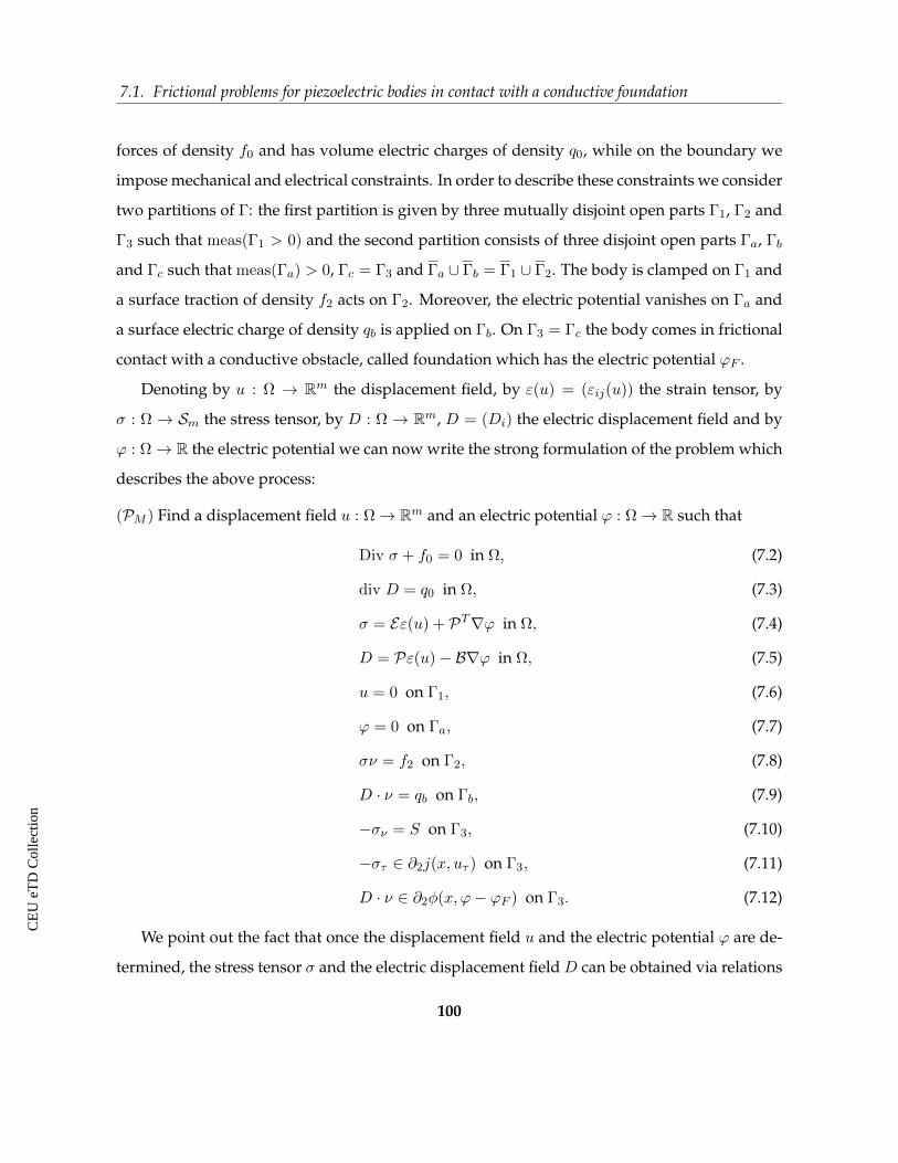
CE
UeT
DC
olle
ctio
n
7.1. Frictional problems for piezoelectric bodies in contact with a conductive foundation
forces of density f0 and has volume electric charges of density q0, while on the boundary we
impose mechanical and electrical constraints. In order to describe these constraints we consider
two partitions of Γ: the first partition is given by three mutually disjoint open parts Γ1, Γ2 and
Γ3 such that meas(Γ1 > 0) and the second partition consists of three disjoint open parts Γa, Γb
and Γc such that meas(Γa) > 0, Γc = Γ3 and Γa ∪ Γb = Γ1 ∪ Γ2. The body is clamped on Γ1 and
a surface traction of density f2 acts on Γ2. Moreover, the electric potential vanishes on Γa and
a surface electric charge of density qb is applied on Γb. On Γ3 = Γc the body comes in frictional
contact with a conductive obstacle, called foundation which has the electric potential ϕF .
Denoting by u : Ω → Rm the displacement field, by ε(u) = (εij(u)) the strain tensor, by
σ : Ω → Sm the stress tensor, by D : Ω → Rm, D = (Di) the electric displacement field and by
ϕ : Ω→ R the electric potential we can now write the strong formulation of the problem which
describes the above process:
(PM ) Find a displacement field u : Ω→ Rm and an electric potential ϕ : Ω→ R such that
Div σ + f0 = 0 in Ω, (7.2)
div D = q0 in Ω, (7.3)
σ = Eε(u) + PT∇ϕ in Ω, (7.4)
D = Pε(u)− B∇ϕ in Ω, (7.5)
u = 0 on Γ1, (7.6)
ϕ = 0 on Γa, (7.7)
σν = f2 on Γ2, (7.8)
D · ν = qb on Γb, (7.9)
−σν = S on Γ3, (7.10)
−στ ∈ ∂2j(x, uτ ) on Γ3, (7.11)
D · ν ∈ ∂2φ(x, ϕ− ϕF ) on Γ3. (7.12)
We point out the fact that once the displacement field u and the electric potential ϕ are de-
termined, the stress tensor σ and the electric displacement field D can be obtained via relations
100
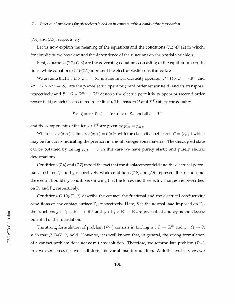
CE
UeT
DC
olle
ctio
n
7.1. Frictional problems for piezoelectric bodies in contact with a conductive foundation
(7.4) and (7.5), respectively.
Let us now explain the meaning of the equations and the conditions (7.2)-(7.12) in which,
for simplicity, we have omitted the dependence of the functions on the spatial variable x.
First, equations (7.2)-(7.3) are the governing equations consisting of the equilibrium condi-
tions, while equations (7.4)-(7.5) represent the electro-elastic constitutive law.
We assume that E : Ω × Sm → Sm is a nonlinear elasticity operator, P : Ω × Sm → Rm and
PT : Ω × Rm → Sm are the piezoelectric operator (third order tensor field) and its transpose,
respectively and B : Ω × Rm → Rm denotes the electric permittivity operator (second order
tensor field) which is considered to be linear. The tensors P and PT satisfy the equality
Pτ · ζ = τ : PT ζ, for all τ ∈ Sm and all ζ ∈ Rm
and the components of the tensor PT are given by pTijk = pkij .
When τ 7→ E(x, τ) is linear, E(x, τ) = C(x)τ with the elasticity coefficients C = (cijkl) which
may be functions indicating the position in a nonhomogeneous material. The decoupled state
can be obtained by taking pijk = 0, in this case we have purely elastic and purely electric
deformations.
Conditions (7.6) and (7.7) model the fact that the displacement field and the electrical poten-
tial vanish on Γ1 and Γa, respectively, while conditions (7.8) and (7.9) represent the traction and
the electric boundary conditions showing that the forces and the electric charges are prescribed
on Γ2 and Γb, respectively.
Conditions (7.10)-(7.12) describe the contact, the frictional and the electrical conductivity
conditions on the contact surface Γ3, respectively. Here, S is the normal load imposed on Γ3,
the functions j : Γ3 × Rm → Rm and φ : Γ3 × R → R are prescribed and ϕF is the electric
potential of the foundation.
The strong formulation of problem (PM ) consists in finding u : Ω → Rm and ϕ : Ω → R
such that (7.2)-(7.12) hold. However, it is well known that, in general, the strong formulation
of a contact problem does not admit any solution. Therefore, we reformulate problem (PM )
in a weaker sense, i.e. we shall derive its variational formulation. With this end in view, we
101
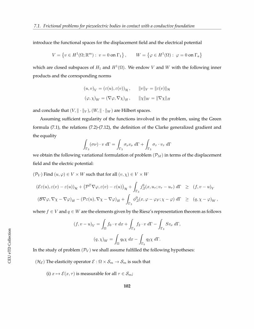
CE
UeT
DC
olle
ctio
n
7.1. Frictional problems for piezoelectric bodies in contact with a conductive foundation
introduce the functional spaces for the displacement field and the electrical potential
V =v ∈ H1(Ω;Rm) : v = 0 on Γ1
, W =
ϕ ∈ H1(Ω) : ϕ = 0 on Γa
which are closed subspaces of H1 and H1(Ω). We endow V and W with the following inner
products and the corresponding norms
(u, v)V = (ε(u), ε(v))H , ‖v‖V = ‖ε(v)‖H
(ϕ, χ)W = (∇ϕ,∇χ)H , ‖χ‖W = ‖∇χ‖H
and conclude that (V, ‖ · ‖V ), (W, ‖ · ‖W ) are Hilbert spaces.
Assuming sufficient regularity of the functions involved in the problem, using the Green
formula (7.1), the relations (7.2)-(7.12), the definition of the Clarke generalized gradient and
the equality ∫Γ3
(σν) · v dΓ =
∫Γ3
σνvν dΓ +
∫Γ3
στ · vτ dΓ
we obtain the following variational formulation of problem (PM ) in terms of the displacement
field and the electric potential:
(PV ) Find (u, ϕ) ∈ V ×W such that for all (v, χ) ∈ V ×W
(Eε(u), ε(v)− ε(u))H +(PT∇ϕ, ε(v)− ε(u)
)H +
∫Γ3
j0,2(x, uτ ; vτ − uτ ) dΓ ≥ (f, v − u)V
(B∇ϕ,∇χ−∇ϕ)H − (Pε(u),∇χ−∇ϕ)H +
∫Γ3
φ0,2(x, ϕ− ϕF ;χ− ϕ) dΓ ≥ (q, χ− ϕ)W ,
where f ∈ V and q ∈W are the elements given by the Riesz’s representation theorem as follows
(f, v − u)V =
∫Ωf0 · v dx+
∫Γ2
f2 · v dΓ−∫
Γ3
Svν dΓ,
(q, χ)W =
∫Ωq0χ dx−
∫Γb
q2χ dΓ.
In the study of problem (PV ) we shall assume fulfilled the following hypotheses:
(HE) The elasticity operator E : Ω× Sm → Sm is such that
(i) x 7→ E(x, τ) is measurable for all τ ∈ Sm;
102
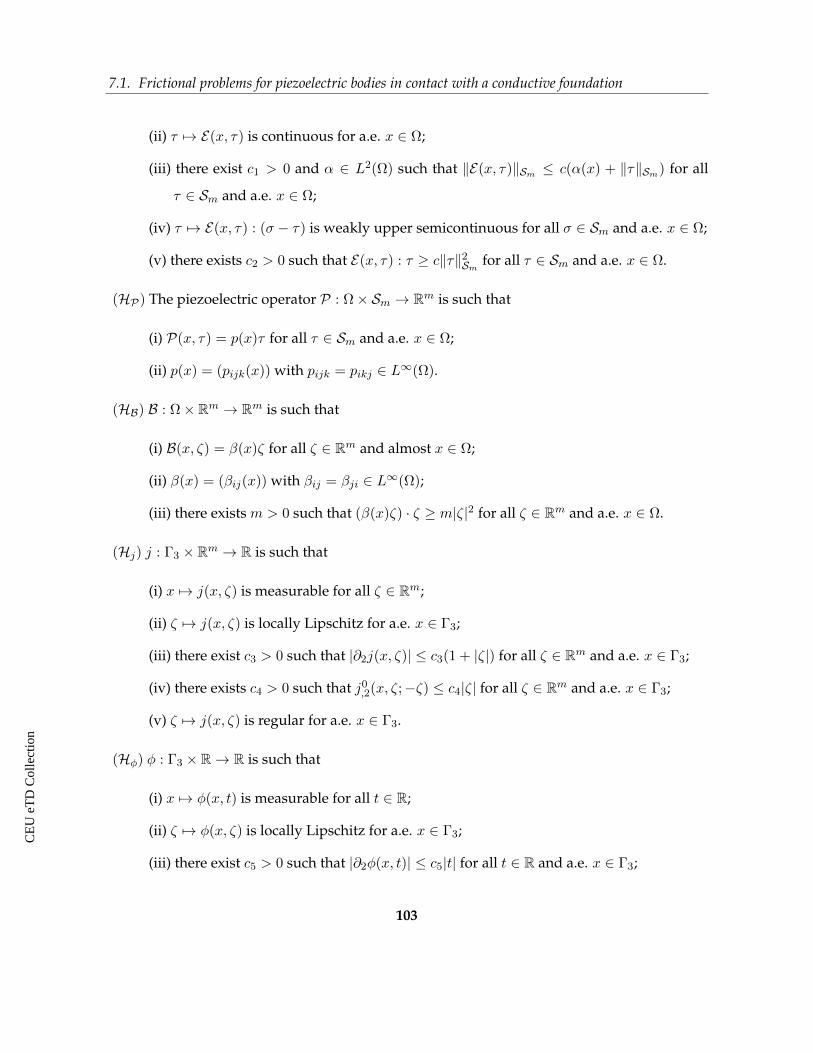
CE
UeT
DC
olle
ctio
n
7.1. Frictional problems for piezoelectric bodies in contact with a conductive foundation
(ii) τ 7→ E(x, τ) is continuous for a.e. x ∈ Ω;
(iii) there exist c1 > 0 and α ∈ L2(Ω) such that ‖E(x, τ)‖Sm ≤ c(α(x) + ‖τ‖Sm) for all
τ ∈ Sm and a.e. x ∈ Ω;
(iv) τ 7→ E(x, τ) : (σ − τ) is weakly upper semicontinuous for all σ ∈ Sm and a.e. x ∈ Ω;
(v) there exists c2 > 0 such that E(x, τ) : τ ≥ c‖τ‖2Sm for all τ ∈ Sm and a.e. x ∈ Ω.
(HP) The piezoelectric operator P : Ω× Sm → Rm is such that
(i) P(x, τ) = p(x)τ for all τ ∈ Sm and a.e. x ∈ Ω;
(ii) p(x) = (pijk(x)) with pijk = pikj ∈ L∞(Ω).
(HB) B : Ω× Rm → Rm is such that
(i) B(x, ζ) = β(x)ζ for all ζ ∈ Rm and almost x ∈ Ω;
(ii) β(x) = (βij(x)) with βij = βji ∈ L∞(Ω);
(iii) there exists m > 0 such that (β(x)ζ) · ζ ≥ m|ζ|2 for all ζ ∈ Rm and a.e. x ∈ Ω.
(Hj) j : Γ3 × Rm → R is such that
(i) x 7→ j(x, ζ) is measurable for all ζ ∈ Rm;
(ii) ζ 7→ j(x, ζ) is locally Lipschitz for a.e. x ∈ Γ3;
(iii) there exist c3 > 0 such that |∂2j(x, ζ)| ≤ c3(1 + |ζ|) for all ζ ∈ Rm and a.e. x ∈ Γ3;
(iv) there exists c4 > 0 such that j0,2(x, ζ;−ζ) ≤ c4|ζ| for all ζ ∈ Rm and a.e. x ∈ Γ3;
(v) ζ 7→ j(x, ζ) is regular for a.e. x ∈ Γ3.
(Hφ) φ : Γ3 × R→ R is such that
(i) x 7→ φ(x, t) is measurable for all t ∈ R;
(ii) ζ 7→ φ(x, ζ) is locally Lipschitz for a.e. x ∈ Γ3;
(iii) there exist c5 > 0 such that |∂2φ(x, t)| ≤ c5|t| for all t ∈ R and a.e. x ∈ Γ3;
103
CE
UeT
DC
olle
ctio
n
7.1. Frictional problems for piezoelectric bodies in contact with a conductive foundation
(iv) t 7→ φ(x, t) is regular for a.e. x ∈ Γ3.
(Hf,q) f0 ∈ H , f2 ∈ L2(Γ2;Rm), q0 ∈ L2(Ω), qb ∈ L2(Γ2), S ∈ L∞(Γ3), S ≥ 0, ϕF ∈ L2(Γ3).
The main result of this subsection is given by the following theorem.
Theorem 7.1. (N.C. & C. VARGA [38]) Assume fulfilled conditions (HE), (HP), (HB), (Hj), (Hφ)
and (Hf,q). Then problem (PV ) admits at least one solution.
Proof. We observe that problem (PV ) is in fact a system of two coupled hemivariational in-
equalities. The idea is to apply one of the existence results obtained in Section 2. with suitable
choice of ψk, J , and Fk (k ∈ 1, 2).
First, let us take n = 2 and defineX1 = V , X2 = W , Y1 = L2(Γ3;Rm), Y2 = L2(Γ3), K1 = X1
and K2 = X2. Next we introduce T1 : X1 → Y1 and T2 : X2 → Y2 defined by
T1 = iτ γm im|Γ3 , T2 = γ i|Γ3 ,
where im : V → H1 = H1(Ω;Rm) is the embedding operator, γm : H1 → H1/2(Γ;Rm) is the
Sobolev trace operator, iτ : H1/2(Γ;Rm)→ L2(Γ3;Rm) is the operator defined by iτ (v) = vτ , i :
W → H1(Ω) is the embedding operator and γ : H1(Ω)→ H1/2(Γ) is the Sobolev trace operator.
Clearly T1 and T2 are linear and compact operators. We consider next ψ1 : X1 ×X2 ×X1 → R
and ψ2 : X1 ×X2 ×X2 → R defined by
ψ1(u, ϕ, v) = (Eε(u), ε(v)− ε(u))H +(PT∇ϕ, ε(v)− ε(u)
)H ,
ψ2(u, ϕ, χ) = (B∇ϕ,∇χ−∇ϕ)H − (Pε(u),∇χ−∇ϕ)H ,
J : Y1 × Y2 → R defined by
J(w, η) =
∫Γ3
j(x,w(x)) dΓ +
∫Γ3
φ(x, η(x)− ϕ(x)) dΓ,
and F1 : X1 ×X2 → X∗1 and F2 : X1 ×X2 → X∗2 defined by
F1(u, ϕ) = f, F2(u, ϕ) = q.
104
CE
UeT
DC
olle
ctio
n
7.2. The bipotential method for contact problems with nonmonotone boundary conditions
It is easy to infer from the above definitions that if (HE), (HP), (HB) hold, then the functionals
ψ1, ψ2 satisfy conditions (H1) and (H6). Taking (Hj) and (Hφ) into account we conclude that J
is a regular locally Lipschitz functional which satisfies
J0,1(w, η; z) =
∫Γ3
j0,2(x,w(x); z(x)) dΓ
J0,2(w, η; ζ) =
∫Γ3
φ0,2(x, η(x)− ϕ(x); ζ(x)) dΓ.
Obviously conditions (H2), (H7), (H8) are fulfilled, therefore we can apply Corollary 6.2 to
conclude that problem (PV ) admits at least one solution.
7.2 The bipotential method for contact problems with nonmonotone
boundary conditions
This section focuses on the weak solvability of a general mathematical model which describes
the contact between a body and an obstacle. The process is assumed to be static and we work
under the small deformations hypothesis. The behavior of the materials is described by a pos-
sibly multivalued constitutive law written as a subdifferential inclusion, while the contact be-
tween the body and the foundation is described by two inclusions, corresponding to the normal
and the tangential directions, each inclusion involving the sum of a Clarke subdifferential and
the normal cone of a nonempty, closed and convex set.
Inspired and motivated by some recent papers in the literature we consider a variational
formulation in terms of bipotentials for our model. This leads to a system of two inequalities:
a hemivariational inequality related to the equilibrium law and a variational inequality related
to the functional extension of the constitutive law. The unknown of the system is a pair (u, σ)
consisting of the displacement field and the Cauchy stress field. A key role in our approach is
played by the separable bipotential that can be defined as the sum of the constitutive map and
its Fenchel conjugate. Bipotentials were introduced in 1991 by de Saxcé & Feng [110] and within
a very short period of time this theory has undergone a remarkable development both in pure
105
CE
UeT
DC
olle
ctio
n
7.2. The bipotential method for contact problems with nonmonotone boundary conditions
and applied mathematics as bipotentials were successfully applied in addressing various prob-
lems arising in mechanics (non-associated Drücker-Prager models in plasticity [18, 114], cam-
clay models in soil mechanics [113, 124], cyclic plasticity [11, 112] and viscoplasticity of metals
with kinematical hardening rule [58], Coulomb’s friction law [15, 70, 78], displacement-traction
models for elastic materials [79], contact models with Signorini’s boundary condition [77]). For
more details and connections regarding the theory of bipotentials see also [16, 17, 115]. The
bipotential approach has the advantage that it allows to approximate simultaneously the dis-
placement field and the Cauchy stress tensor and facilitated the implementation of new and
efficient numerical algorithms (see e.g. [51, 111]). However, in all the works we are aware
of, the bipotential method has been used only for problems with monotone boundary con-
ditions, mostly expressed as inclusions involving the subdifferential of a proper, convex and
lower semicontinuous function. Thus, the variational formulation for these problems leads to
a coupled system of variational inequalities. In this paper, due to the nonmonotone boundary
conditions two major differences arise:
• the set of admissible stress tensors is defined with respect to a given displacement field and
depends explicitly on this displacement field, in contrast to the case of monotone bound-
ary conditions when the set of admissible stress tensors is the same for all displacement
fields;
• the variational formulation leads to a system of inequalities consisting of a hemivariational
inequality and a variational inequality.
Consequently, several difficulties occur in determining the existence of weak solutions since
the classical methods fail to be applied directly.
7.2.1 The mechanical model and its variational formulation
Let us consider a body B which occupies the domain Ω ⊂ Rm (m = 2, 3) with a sufficiently
smooth boundary Γ (e.g. Lipschitz continuous) and a unit outward normal ν. The body is
acted upon by forces of density f0 and it is mechanically constrained on the boundary. In order
106
CE
UeT
DC
olle
ctio
n
7.2. The bipotential method for contact problems with nonmonotone boundary conditions
to describe these constraints we assume Γ is partitioned into three Lebesgue measurable parts
Γ1,Γ2,Γ3 such that Γ1 has positive Lebesgue measure. The body is clamped on Γ1, hence the
displacement field vanishes here, while surface tractions of density f2 act on Γ2. On Γ3 the body
may come in contact with an obstacle which will be referred to as foundation. The process is
assumed to be static and the behavior of the material is modeled by a (possibly multivalued)
constitutive law expressed as a subdifferential inclusion. The contact between the body and
the foundation is modeled with respect to the normal and the tangent direction respectively,
to each corresponding an inclusion involving the sum between the Clarke subdifferential of a
locally Lipschitz function and the normal cone of a nonempty, closed and convex set.
It is well known that the subdifferential of a convex function is a monotone set-valued
operator, while the Clarke subdifferential is a set-valued operator which is not monotone in
general. This is why we say that the constitutive law is monotone and the boundary conditions
are nonmonotone.
The mathematical model which describes the above process is the following. For simplicity
we omit the dependence of some functions of the spatial variable.
(P) Find a displacement u : Ω→ Rm and a stress tensor σ : Ω→ Sm such that
−Div σ = f0, in Ω (7.13)
σ ∈ ∂φ(ε(u)), a.e. in Ω (7.14)
u = 0, on Γ1 (7.15)
σν = f2, on Γ2 (7.16)
−σν ∈ ∂2Cjν(x, uν) +NC1(uν), on Γ3 (7.17)
−στ ∈ h(x, uτ )∂2Cjτ (x, uτ ) +NC2(uτ ), on Γ3 (7.18)
where φ : Sm → R is convex and lower semicontinous, jν : Γ3 × R→ R and jτ : Γ3 × Rm → R
are locally Lipschitz with respect to the second variable and h : Γ3 × Rm → R is a prescribed
function. Here,C1 ⊂ R andC2 ⊂ Rm are nonempty closed and convex subsets andNCk denotes
the normal cone of Ck (k = 1, 2). For a Banach space E and a nonempty, closed and convex
107

CE
UeT
DC
olle
ctio
n
7.2. The bipotential method for contact problems with nonmonotone boundary conditions
subset K ⊂ E, the normal cone of K at x is defined by
NK(x) =ξ ∈ E∗ : 〈ξ, y − x〉E∗×E ≤ 0, for all y ∈ K
.
It is well known that
NK(x) = ∂IK(x),
where IK is the indicator function of K, that is,
IK(x) =
0, if x ∈ K,
+∞, otherwise.
Relation (7.13) represents the equilibrium equation, (7.14) is the constitutive law, (7.15)-
(7.16) are the displacement and traction boundary conditions and (7.17)-(7.18) describe the
contact between body and the foundation.
Relations between the stress tensor σ and the strain tensor ε of the type (7.14) describe
the constitutive laws of the deformation theory of plasticity, of Hencky plasticity with convex
yield function, of locking materials with convex locking functions etc. For concrete examples
and their physical interpretation one can consult Sections 3.3.1 and 3.3.2 in Panagiotopoulos
[98] (see also Section 3.1 in [99]). A particular case of interest regarding (7.14) is when the
constitutive map φ is Gâteaux differentiable, thus the subdifferential inclusion reduces to
σ = φ′(ε(u)), (7.19)
which corresponds to nonlinear elastic materials.
Some classical constitutive laws which can be written in the form (7.19) are presented below:
(i) Assume that φ is defined by
φ(µ) =1
2Eµ : µ,
where E = (Eijkl), 1 ≤ i, j, k, l ≤ m is a fourth order tensor which satisfies the symmetry
property
Eµ : τ = µ : Eτ, for all µ, τ ∈ Sm,
108
CE
UeT
DC
olle
ctio
n
7.2. The bipotential method for contact problems with nonmonotone boundary conditions
and the ellipticity property
Eµ : µ ≥ c|µ|2, for all µ ∈ Sm.
In this case (7.19) reduces to Hooke’s law, that is, σ = Eε(u), and corresponds to linearly
elastic materials.
(ii) Assume that φ is defined by
φ(µ) =1
2Eµ : µ+ β |µ− PKµ|2 ,
where E is the elasticity tensor and satisfies the same properties as in the previous exam-
ple, β > 0 is a constant coefficient of the material, P : Sm → K is the projection operator
and K is the nonempty, closed and convex von Mises set
K =
µ ∈ Sm :
1
2µD : µD ≤ a2, a > 0
.
Here the notation µD stands for the deviator of the tensor µ, that is, µD = µ − 1mTr(µ)I ,
with I being the identity tensor.
In this case (7.19) becomes
σ = Eε(u) + 2β(I − PK)ε(u),
which is known in the literature as the piecewise linear constitutive law (see e.g. Han &
Sofonea [56]).
(iii) Assume φ is defined by
φ(µ) =k0
2Tr(µ)I : µ+
1
2ϕ(∣∣µD∣∣2) ,
where k0 > 0 is a constant and ϕ : [0,∞)→ [0,∞) is a continuously differentiable consti-
tutive function.
In this case (7.19) becomes
σ = k0Tr(ε(u))I + ϕ′(∣∣εD(u)
∣∣2) εD(u),
and this describes the behavior of the Hencky materials (see e.g. Zeidler [122]).
109
CE
UeT
DC
olle
ctio
n
7.2. The bipotential method for contact problems with nonmonotone boundary conditions
Boundary conditions of the type (7.17) and (7.18) model a large class of contact problems arising
in mechanics and engineering. For the case h ≡ 1 many examples of nonmonotone laws of the
type
−σν ∈ ∂Cjν(uν) and − στ ∈ ∂Cjτ (uτ ),
can be found in [99] Section 2.4, [94] Section 1.4 or [53] Section 2.8.
The case when the function h actually depends on the second variable allows the study of
contact problems with slip-dependent friction law (see e.g. [29, 80] for antiplane models and [30]
for general 3D models). This friction law reads as follows
−στ ≤ µ(x, |uτ |), −στ = µ(x, |uτ |)uτ|uτ |
if uτ 6= 0, (7.20)
where µ : Γ3 × [0,+∞)→ [0,+∞) is the sliding threshold and it is assumed to satisfy
0 ≤ µ(x, t) ≤ µ0, for a.e. x ∈ Γ3 and all t ≥ 0,
for some positive constant µ0. It is easy to see that (7.18) can be put in the form (7.20) simply
by choosing
h(x, uτ ) = µ(x, |uτ |) and jτ (x, uτ ) = |uτ |.
We point out the fact that the above example cannot be written in the form −στ ∈ ∂Cjτ (uτ ) as,
in general, for two locally Lipschitz functions h, g there does not exists j such that ∂Cj(u) =
h(u)∂Cg(u). We would also like to point out that many boundary conditions of classical elastic-
ity are particular cases of (7.17) and (7.18), in most of these cases the functions jν and jτ being
convex, hence leading to monotone boundary conditions. We list below some examples:
(a) The Winkler boundary condition
−σν = k0uν , k0 > 0.
This law is used in engineering as it describes the interaction between a deformable body
and the soil and can be expressed in the form (7.17) by setting
C1 = R and jν(x, uν) =k0
2u2ν .
110
CE
UeT
DC
olle
ctio
n
7.2. The bipotential method for contact problems with nonmonotone boundary conditions
More generally, if we want to describe the case when the body may lose contact with the
foundation, we can consider the following law uν < 0⇒ σν = 0,
uν ≥ 0⇒ −σν = k0uν .
The first relation corresponds to the case when there is no contact, while the second mod-
els the contact case. Obviously the above law can be expressed in the form (7.17) by
choosing
C1 = R and jν(x, uν) =
0, if uν < 0,
k02 u
2ν , if uν ≥ 0.
In [93] the following nonmonotone boundary conditions were imposed to model the con-
tact between a body and a Winkler-type foundation which may sustain limited values of
efforts
uν < 0⇒ σν = 0,
uν ∈ [0, a)⇒ −σν = k0uν ,
uν = a⇒ −σν ∈ [0, k0a],
uν > a⇒ σν = 0.
This means that the rupture of the foundation is assumed to occur at those points in which
the limit effort is attained. The first condition holds in the noncontact zone, the second
describes the zone where the contact occurs and it is idealized by the Winkler law. The
maximal value of reactions that can be maintained by the foundation is given by k0a and
it is accomplished when uν = a, with k0 being the Winkler coefficient. The fourth relation
holds in the zone where the foundation has been destroyed. The above Winkler-type law
can be written as an inclusion of the type (7.17) by setting
C1 = R and jν(x, uν) =
0, if uν < 0,
k02 u
2ν , if 0 ≤ uν < a,
k02 a
2, if uν ≥ a.
111
CE
UeT
DC
olle
ctio
n
7.2. The bipotential method for contact problems with nonmonotone boundary conditions
Since all of the above examples only describe what happens in the normal direction, in
order to complete the model we must combine these with boundary conditions concern-
ing στ , uτ , or both. The simplest cases are uτ = 0 (which corresponds to C2 = 0) and
στ = Sτ , where Sτ = Sτ (x) is given (which corresponds to jτ (x, uτ ) = −Sτ · uτ ).
(b) The Signorini boundary conditions, which hold if the foundation is rigid and are as follows uν < 0⇒ σν = 0,
uν = 0⇒ σν ≤ 0,
or equivalently,
uν ≤ 0, σν ≤ 0 and σνuν = 0.
This can be written equivalently in form (7.17) by setting
C1 = (−∞, 0] and jν ≡ 0.
(c) In [78] the following static version of Coulomb’s law of dry friction with prescribed normal stress
was considered −σν(x) = F (x)
|στ | ≤ k(x)|σν |,
στ = −k(x)|σν | uτ|uτ | , if uτ (x) 6= 0.
We can write the above law in the form of (7.17) and (7.18) simply by setting
C1 = R, C2 = Rm, jν(x, uν) = F (x)uν , h(x, uτ ) = k(x)|F (x)| and jτ (x, uτ ) = |uτ |.
The assumptions on the functions f0, f2, φ, h, jν and jτ required to prove our main result are
listed below.
(HC) The constraint sets C1 and C2 are convex cones, i.e.
0 ∈ Ck and λCk ⊂ Ck for all λ > 0, k = 1, 2.
112
CE
UeT
DC
olle
ctio
n
7.2. The bipotential method for contact problems with nonmonotone boundary conditions
(Hf ) The density of the volume forces and the traction satisfy f0 ∈ H and f2 ∈ L2(Γ2;Rm).
(Hφ) The constitutive function φ : Sm → R and its Fenchel conjugate φ∗ : Sm → (−∞,+∞]
satisfy
(i) φ is convex and lower semicontinuous;
(ii) there exists α1 > 0 such that φ(τ) ≥ α1|τ |2, for all τ ∈ Sm;
(iii) there exists α2 > 0 such that φ∗(µ) ≥ α2|µ|2, for all µ ∈ Sm;
(iv) φ(ε(v)) ∈ L1(Ω), for all v ∈ V and φ∗(τ) ∈ L1(Ω), for all τ ∈ H.
(Hh) The function h : Γ3 × Rm → R is such that
(i) Γ3 3 x 7→ h(x, ζ) is measurable for each ζ ∈ Rm;
(ii) Rm 3 ζ 7→ h(x, ζ) is continuous for a.e. x ∈ Γ3;
(iii) there exists h0 > 0 such that 0 ≤ h(x, ζ) ≤ h0 for a.e. x ∈ Γ3 and all ζ ∈ Rm.
(Hjν ) The function jν : Γ3 × R→ R is such that
(i) Γ3 3 x 7→ jν(x, t) is measurable for each t ∈ R;
(ii) there exists p ∈ L2(Γ3) such that for a.e. x ∈ Γ3 and all t1, t2 ∈ R
|jν(x, t1)− jν(x, t2)| ≤ p(x)|t1 − t2|;
(iii) jν(x, 0) ∈ L1(Γ3).
(Hjτ ) The function jτ : Γ3 × Rm → R is such that
(i) Γ3 3 x 7→ jτ (x, ζ) is measurable for each ζ ∈ Rm;
(ii) there exist q ∈ L2(Γ3) such that for a.e. x ∈ Γ3 and all ζ2, ζ2 ∈ Rm
|jτ (x, ζ1)− jτ (x, ζ2)| ≤ q(x)|ζ1 − ζ2|;
113
CE
UeT
DC
olle
ctio
n
7.2. The bipotential method for contact problems with nonmonotone boundary conditions
(iii) jτ (x, 0) ∈ L1(Γ3;Rm).
The strong formulation of problem (P) consists in finding u : Ω → Rm and σ : Ω → Sm,
regular enough, such that (7.13)-(7.18) are satisfied. However, it is a fact that for most contact
problems the strong formulation has no solution. Therefore, it is useful to reformulate problem
(P) in a weaker sense, i.e. we shall derive a variational formulation. With this end in mind, we
consider the following function space
V = v ∈ H1 : v = 0 a.e. on Γ1 (7.21)
which is a closed subspace of H1, hence a Hilbert space. Since the Lebesgue measure of Γ1 is
positive, it follows from Korn’s inequality that the following inner product
(u, v)V = (ε(u), ε(v))H (7.22)
generates a norm on V which is equivalent with the norm inherited from H1.
Let us provide a variational formulation for problem (P). To this end, we consider u a
strong solution, v ∈ V a test function and we multiply the first line of (P) by v − u. Using the
Green formula (7.1) we have
(f0, v − u)H = − (Div σ, v − u)H
= −∫
Γ(σν) · (v − u) dΓ + (σ, ε(v)− ε(u))H
= −∫
Γ2
f2 · (v − u) dΓ−∫
Γ3
[σν(vν − uν) + στ · (vτ − uτ )] dΓ + (σ, ε(v)− ε(u))H
for all v ∈ V . Since V 3 v 7→ (f0, v)H +∫
Γ2f2 · v dΓ is linear and continuous, we can apply
Riesz’s representation theorem to conclude that there exists a unique element f ∈ V such that
(f, v)V = (f0, v)H +
∫Γ2
f2 · v dΓ. (7.23)
Consider now the following nonempty, closed and convex subset of V
Λ = v ∈ V : vν(x) ∈ C1 and vτ (x) ∈ C2 for a.e. x ∈ Γ3 ,
114

CE
UeT
DC
olle
ctio
n
7.2. The bipotential method for contact problems with nonmonotone boundary conditions
which is called the set of admissible displacement fields.
Since C1, C2 are convex cones, it follows that Λ is also a convex cone. Moreover, taking into
account Definitions 1.7 and 1.8, we deduce that for all v ∈ Λ the following inequalities hold
−∫
Γ3
σν(vν − uν) dΓ ≤∫
Γ3
j0ν(x, uν ; vν − uν) dΓ (7.24)
and
−∫
Γ3
στ · (vτ − uτ ) dΓ ≤∫
Γ3
h(x, uτ )j0τ (x, uτ ; vτ − uτ ) dΓ. (7.25)
Here, and hereafter, the generalized derivatives of the functions jν and jτ are taken with
respect to the second variable, i.e. of the functions R 3 t 7→ jν(x, t) and Rm 3 ζ 7→ jτ (x, ζ)
respectively, but for simplicity we omit to mention that in fact these are partial generalized
derivatives. On the other hand, taking Proposition 1.2 into account we can rewrite (7.14) as
ε(u) ∈ ∂φ∗(σ), a.e. in Ω,
and which after integration over Ω leads to
−(ε(u), µ− σ)H +
∫Ωφ∗(µ)− φ∗(σ) dx ≥ 0, for all µ ∈ H. (7.26)
Let us define the operator L : V → H by Lv = ε(v) and denote by L∗ : H → V its adjoint, that
is,
(L∗µ, v)V = (µ,Lv)H, for all v ∈ V and all µ ∈ H.
Using (7.23)-(7.26) we arrive at the following system of inequalities
(P) Find u ∈ Λ and σ ∈ H such that
(L∗σ, v − u)V +
∫Γ3
[j0ν(x, uν ; vν − uν) + h(x, uτ )j0
τ (x, uτ ; vτ − uτ )]dΓ ≥ (f, v − u)V , (7.27)
−(Lu, µ− σ)H +
∫Ωφ∗(µ)− φ∗(σ) dx ≥ 0, (7.28)
for all (v, µ) ∈ Λ×H.
The inequality (7.27) is related to the equilibrium relation, while (7.28) represents the func-
tional extension of the constitutive law (7.14). It is well-known (see e.g. [53], Theorem 1.3.21)
that relation (7.28) implies Lu ∈ ∂φ∗(σ) a.e. where in Ω.
115

CE
UeT
DC
olle
ctio
n
7.2. The bipotential method for contact problems with nonmonotone boundary conditions
Proposition 1.2 allows us to construct the separable bipotential a : Sm × Sm → (−∞,+∞],
which connects the constitutive law, the function φ and its conjugate φ∗, as follows
a(τ, µ) = φ(τ) + φ∗(µ), for all τ, µ ∈ Sm.
Using the bipotential a let us define A : V ×H → R by
A(v, µ) =
∫Ωa(Lv, µ) dx, for all v ∈ V, µ ∈ H.
and note that, due to (Hφ), A is well defined and
A(v, µ) ≥ α1‖v‖2V + α2‖µ‖2H, for all v ∈ V, µ ∈ H.
Moreover, Proposition 1.2 ensures that
A(u, σ) = (L∗σ, u)V and A(v, µ) ≥ (L∗µ, v)V , for all v ∈ V, µ ∈ H. (7.29)
Combining (7.27) and (7.29) we get
A(v, σ)−A(u, σ) +
∫Γ3
[j0ν(x, uν ; vν − uν) + h(x, uτ )j0
τ (x, uτ ; vτ − uτ )]dΓ ≥ (f, v−u)V , (7.30)
for all v ∈ Λ.
Let us define now the set of admissible stress tensors with respect to the displacement u, to be the
following subset ofH
Θu =
µ ∈ H : (L∗µ, v)V +
∫Γ3
[j0ν(x, uν ; vν) + h(x, uτ )j0
τ (x, uτ ; vτ )]dΓ ≥ (f, v)V , ∀v ∈ Λ
.
Let w ∈ Λ be fixed. Choosing v = u + w ∈ Λ in (7.27) shows that σ ∈ Θu, hence Θu 6= ∅. It
is easy to check that Θu is an unbounded, closed and convex subset of H. Taking into account
(7.29) we have
A(u, µ) +
∫Γ3
[j0ν(x, uν ;uν) + h(x, uτ )j0
τ (x, uτ ;uτ )]dΓ ≥ (f, u)V , for all µ ∈ Θu,
while for v = 0 ∈ Λ in (7.27) we have
−A(u, σ) +
∫Γ3
[j0ν(x, uν ;−uν) + h(x, uτ )j0
τ (x, uτ ;−uτ )]dΓ ≥ −(f, u)V .
116
CE
UeT
DC
olle
ctio
n
7.2. The bipotential method for contact problems with nonmonotone boundary conditions
Adding the above relations, for all µ ∈ Θu we have
0 ≤ A(u, µ)−A(u, σ) +
∫Γ3
j0ν(x, uν ;uν) + j0
ν(x, uν ;−uν)dΓ
+
∫Γ3
h(x, uτ )(j0τ (x, uτ ;uτ ) + j0
τ (x, uτ ;−uτ ))dΓ.
On the other hand, Proposition 1.3 and (Hh) ensure that∫Γ3
[j0ν(x, uν ;uν) + j0
ν(x, uν ;−uν) + h(x, uτ )(j0τ (x, uτ ;uτ ) + j0
τ (x, uτ ;−uτ ))]
dΓ ≥ 0. (7.31)
(Pbvar
)Find u ∈ Λ and σ ∈ Θu such that A(v, σ)−A(u, σ) +
∫Γ3
[j0ν(x, uν ; vν − uν) + h(x, uτ )j0
τ (x, uτ ; vτ − uτ )]dΓ ≥ (f, v − u)V ,
A(u, µ)−A(u, σ) ≥ 0,
for all (v, µ) ∈ Λ×Θu.
Each solution (u, σ) ∈ Λ×Θu of problem(Pbvar
)is called a weak solution for problem (P).
7.2.2 The connection with classical variational formulations
In this section we prove an existence result concerning the solutions of problem(Pbvar
)by
using a recent result due to Costea & Varga [38]. First we highlight the connection between the
variational formulation in terms of bipotentials and other variational formulations such as the
primal and dual variational formulations. As we have seen in the previous section, multiplying
the first line of problem (P) by v−u, integrating over Ω and then taking the functional extension
of the constitutive law, we get a coupled system of inequalities, namely problem (P). The
primal variational formulation consists in rewriting (P) as an inequality which depends only
on the displacement field u, while the dual variational formulation consists in rewriting (P) in
terms of the stress tensor σ. The primal variational formulation can be derived by reasoning in
the following way.
The second line of (P) implies that Lu ∈ ∂φ∗(σ) and this can be written equivalently as
σ ∈ ∂φ(Lu), hence
σ : (µ− Lu) ≤ φ(µ)− φ(Lu), for all µ ∈ Sm.
117
CE
UeT
DC
olle
ctio
n
7.2. The bipotential method for contact problems with nonmonotone boundary conditions
For each v ∈ Λ, taking µ = Lv in the previous inequality and integrating over Ω yields
(L∗σ, v − u)V ≤∫
Ωφ(Lv)− φ(Lu) dx, for all v ∈ Λ.
Now, combining the above relation and the first line of (P) we get the following problem
(Ppvar) Find u ∈ Λ such that
F (v)− F (u) +
∫Γ3
[j0ν(x, uν ; vν − uν) + h(x, uτ )j0
τ (x, uτ ; vτ − uτ )]dΓ ≥ (f, v − u)V , ∀v ∈ Λ,
where F : V → R is the convex and lower semicontinous function defined by
F (v) =
∫Ωφ(Lv) dx.
Problem (Ppvar) is called the primal variational formulation of problem (P).
Conversely, in order to transform (P) into a problem formulated in terms of the stress tensor
we reason in the following way. First let us define G : H → R by
G(µ) =
∫Ωφ∗(µ) dx,
and for a fixed w ∈ Λ let Θw be the following subset ofH
Θw =
µ ∈ H : (L∗µ, v)V +
∫Γ3
[j0ν(x,wν ; vν) + h(x,wτ )j0
τ (x,wτ ; vτ )]dΓ ≥ (f, v)V , ∀v ∈ Λ
.
Let us consider the following inclusion(Pdw)
Find σ ∈ H such that
0 ∈ ∂G(σ) + ∂IΘw(σ),
which we call the dual variational formulation with respect to w.
Now, looking at the first line of (P), i.e. relation (7.27), and keeping in mind the above
notations, we deduce that Θu 6= ∅ as σ ∈ Θu. Moreover, for each µ ∈ Θu we have
−(L∗(µ− σ), u)V ≤∫
Γ3
j0ν(x, uν ;uν) + j0
ν(x, uν ;−uν)dΓ
+
∫Γ3
h(x, uτ )(j0τ (x, uτ ;uτ ) + j0
τ (x, uτ ;−uτ ))dΓ,
118
CE
UeT
DC
olle
ctio
n
7.2. The bipotential method for contact problems with nonmonotone boundary conditions
which combined with the second line of (P) leads to
G(µ)−G(σ) ≥ −∫
Γ3
j0ν(x, uν ;uν) + j0
ν(x, uν ;−uν)dΓ
−∫
Γ3
h(x, uτ )(j0τ (x, uτ ;uτ ) + j0
τ (x, uτ ;−uτ ))dΓ,
for all µ ∈ Θu.
A simple computation shows that any solution of(Pdu)
will also solve the above problem.
A particular case of interest regarding problem(Pdw)
is if the set Θw does not actually de-
pend on w. In this case problem(Pdw)
will be simply denoted(Pd)
and will be called the dual
variational formulation of problem (P). For example, this case is encountered when the functions
jν and jτ are convex and positive homogeneous, as it is the case of examples (a)-(c) presented
in the previous section.
In the above particular case, problem(P)
reduces to the following system of variational
inequalities
(P′) Find u ∈ Λ and σ ∈ H such that (L∗σ, v − u)V +H(v)−H(u) ≥ (f, v − u)V , for all v ∈ Λ
− (Lu, µ− σ)H +G(µ)−G(σ) ≥ 0, for all µ ∈ H,
where H = j T , j : L2 (Γ3;Rm)→ R is defined by
j(y) =
∫Γ3
jν(x, yν) + jτ (x, yτ ) dΓ,
and T : V → L2(Γ3;Rm) is given by Tv = [(γ i)(v)]|Γ3 , with i : V → H1 being the embedding
operator and γ : H1 → H1/2(Γ;Rm) being the trace operator. On the other hand, for each
w ∈ Λ,
Θw := Θ = µ ∈ H : (L∗µ, v)V +H(v) ≥ (f, v)V , for all v ∈ Λ ,
and thus by taking v = 2u and v = 0 in the first line of (P′) we get
(L∗σ, u)V +H(u) = (f, u)V ,
119
CE
UeT
DC
olle
ctio
n
7.2. The bipotential method for contact problems with nonmonotone boundary conditions
hence
−(Lu, µ− σ)H ≤ 0, for all µ ∈ Θ.
Combining this and the second line of (P′) we get
G(µ)−G(σ) ≥ 0, for all µ ∈ Θ,
which can be formulated equivalently as(Pd)
Find σ ∈ H such that
0 ∈ ∂G(σ) + ∂IΘ(σ).
7.2.3 The existence of weak solutions
The following proposition points out the connection between the variational formulations pre-
sented above.
Proposition 7.1. A pair (u, σ) ∈ V × H is a solution for(Pbvar
)if and only if u solves (Ppvar) and σ
solves(Pdu).
The main result of this section is given by the following theorem.
Theorem 7.2. (N.C., M. CSIRIK & C. VARGA [26]) Assume (HC), (Hf ), (Hh), (Hjν ), (Hjτ ) and
(Hφ) hold. Then problem(Pbvar
)has at least one solution.
Before proving the main result we need the following Aubin-Clarke type result concerning
the Clarke subdifferential of integral functions. Let us consider the function j : L2 (Γ3;Rm) ×
L2 (Γ3;Rm)→ R defined by
j (y, z) =
∫Γ3
jν (x, zν) + h (x, yτ ) jτ (x, zτ ) dΓ. (7.32)
Lemma 7.1. Assume (Hh), (Hjν ) and (Hjτ ) are fulfilled. Then, for each y ∈ L2(Γ3;Rm), the function
z 7→ j (y, z) is Lipschitz continuous and
j0,2 (y, z; z) ≤
∫Γ3
j0ν (x, zν ; zν) + h (x, yτ ) j0
τ (x, zτ ; zτ ) dΓ. (7.33)
120
CE
UeT
DC
olle
ctio
n
7.2. The bipotential method for contact problems with nonmonotone boundary conditions
In order to prove Theorem 7.2 we consider the following system of nonlinear hemivaria-
tional inequalities.
(SK1,K2) Find (u, σ) ∈ K1 ×K2 such that ψ1(u, σ, v) + J0,1(Tu, Sσ;Tv − Tu) ≥ (F1(u, σ), v − u)X1 , for all v ∈ K1,
ψ2(u, σ, µ) + J0,2(Tu, Sσ;Sµ− Sσ) ≥ (F2(u, σ), µ− σ)X2 , for all µ ∈ K2,
where
• X1 = V , X2 = H, Ki ⊂ Xi is closed and convex (i = 1, 2), Y1 = L2(Γ3;Rm), Y2 = 0;
• ψ1 : X1 ×X2 ×X1 → R is defined by ψ1(u, σ, v) = A(v, σ)−A(u, σ);
• ψ2 : X1 ×X2 ×X2 → R is defined by ψ2(u, σ, µ) = A(u, µ)−A(u, σ);
• T : X1 → Y1 is defined by Tv = [(γ i)(v)]|Γ3 , with i : V → H1 the embedding operator and
γ : H1 → H1/2(Γ;Rm) is the trace operator;
• S : X2 → Y2 is defined by Sτ = 0, for all τ ∈ X2;
• J : Y1× Y2 → R is defined by J(y1, y2
)= j
(y0, y1
), where j : L2(Γ3;Rm)×L2(Γ3;Rm)→ R
is as in (7.32) and y0 is a fixed element of L2(Γ3;Rm);
• F1 : X1 ×X2 → X1 is defined by F1(v, µ) = f ;
• F2 : X1 ×X2 → X2 is defined by F2(v, µ) = 0.
Lemma 7.2. Assume (Hh), (Hjν ), (Hjτ ) and (Hφ) are fulfilled. Then the following statements hold:
(i) ψ1(u, σ, u) = 0 and ψ2(u, σ, σ) = 0, for all (u, σ) ∈ X1 ×X2;
(ii) for each v ∈ X1 and each µ ∈ X2 the maps (u, σ) 7→ ψ1(u, σ, v) and (u, σ) 7→ ψ2(u, σ, µ) are
weakly upper semicontinuous;
(iii) for each (u, σ) ∈ X1 ×X2 the maps v 7→ ψ1(u, σ, v) and µ 7→ ψ2(u, σ, µ) are convex;
(iv) lim infk→+∞
(F1(uk, σk), v − uk)X1 ≥ (F1(u, σ), v − u)X1 and lim infk→+∞
(F2(uk, σk), µ − σk)X2 ≥
(F2(u, σ), µ− σ)X2 whenever (uk, σk) (u, σ) as k → +∞;
121
CE
UeT
DC
olle
ctio
n
7.2. The bipotential method for contact problems with nonmonotone boundary conditions
(v) there exists c : R+ → R+ with the property limt→+∞
c(t) = +∞ such that
ψ1(u, σ, 0)+ψ2(u, σ, 0) ≤ −c(√‖u‖2X1
+ ‖σ‖2X2
)√‖u‖2X1
+ ‖σ‖2X2, for all (u, σ) ∈ X1×X2;
(vi) The function J : Y1 × Y2 → R is Lipschitz with respect to each variable. Moreover, for all(y1, y2
),(z1, z2
)∈ Y1 × Y2 we have
J0,1
(y1, y2; z1
)= j0
,2
(y0, y1; z1
)and
J0,2
(y1, y2; z2
)= 0;
(vii) There exists M > 0 such that
J0,1
(y1, y2;−y1
)≤M
∥∥y1∥∥Y1, for all
(y1, y2
)∈ Y1 × Y2;
(viii) there exist mi > 0, i = 1, 2, such that ‖Fi(u, σ)‖Xi ≤ mi, for all (u, σ) ∈ X1 ×X2.
Proof of Theorem 7.2 The proof will be carried out in three steps as follows.
STEP 1. Let K1 ⊂ X1 and K2 ⊂ X2 be closed and convex sets. Then (SK1,K2) admits at least
one solution.
This will be done by applying a slightly modified version of Corollary 3.7 in [38]. Lemma
7.2 ensures that all the conditions of the aforementioned corollary are satisfied except
the regularity of J . We point out the fact that in our case this condition needs not to be
imposed because the only reason it is imposed in the paper of Costea & Varga is to ensure
the following inequality
J0(y1, y2; z1, z2
)≤ J0
,1
(y1, y2; z1
)+ J0
,2
(y1, y2; z2
)which in this paper is automatically fulfilled because J does not depend on the second
variable and the following equalities take place
J0(y1, y2; z1, z2
)= J0
,1
(y1, y2; z1
)122
CE
UeT
DC
olle
ctio
n
7.2. The bipotential method for contact problems with nonmonotone boundary conditions
and
J0,2
(y1, y2; z2
)= 0,
and this completes the first step.
STEP 2. Let K11 ,K
21 ⊂ X1 and K1
2 ,K22 ⊂ X2 be closed and convex sets and let
(u1, σ1
)and
(u2, σ2
)be solutions for
(SK1
1 ,K12
)and
(SK2
1 ,K22
), respectively. Then
(u1, σ2
)solves(
SK11 ,K
22
)and
(u2, σ1
)solves
(SK2
1 ,K12
).
The fact that(u1, σ1
)solves
(SK1
1 ,K12
)means ψ1(u1, σ1, v) + J0
,1(Tu1, Sσ1;Tv − Tu1) ≥ (F1(u1, σ1), v − u1)X1 , ∀v ∈ K11
ψ2(u1, σ1, µ) + J0,2(Tu1, Sσ1;Sµ− Sσ1) ≥ (F2(u1, σ1), µ− σ1)X2 , ∀µ ∈ K1
2
(7.34)
while the fact that(u2, σ2
)solves
(SK2
1 ,K22
)shows ψ1(u2, σ2, v) + J0
,1(Tu2, Sσ2;Tv − Tu2) ≥ (F1(u2, σ2), v − u2)X1 , ∀v ∈ K21
ψ2(u2, σ2, µ) + J0,2(Tu2, Sσ2;Sµ− Sσ2) ≥ (F2(u2, σ2), µ− σ2)X2 , ∀µ ∈ K2
2
(7.35)
Putting together the first line of (7.34) and the second line of (7.35) we get ψ1(u1, σ1, v) + J0,1(Tu1, Sσ1;Tv − Tu1) ≥ (F1(u1, σ1), v − u1)X1 , ∀v ∈ K1
1
ψ2(u2, σ2, µ) + J0,2(Tu2, Sσ2;Sµ− Sσ2) ≥ (F2(u2, σ2), µ− σ2)X2 , ∀µ ∈ K2
2
(7.36)
On the other hand, keeping in mind the way ψ1, ψ2, J, F1, F2 were defined is it easy to
check that for any (v, µ) ∈ K11 ×K2
2 the following equalities hold
ψ1(u1, σ1, v) = ψ1(u1, σ2, v) and ψ2(u2, σ2, µ) = ψ2(u1, σ2, µ),
J0,1(Tu1, Sσ1;Tv − Tu1) = J0
,1(Tu1, Sσ2;Tv − Tu1)
J0,2(Tu2, Sσ2;Sµ− Sσ2) = J0
,2(Tu1, Sσ2;Sµ− Sσ1)
F1(u1, σ1) = F1(u1, σ2) and F2(u2, σ2) = F2(u1, σ2).
123
CE
UeT
DC
olle
ctio
n
7.2. The bipotential method for contact problems with nonmonotone boundary conditions
Using these equalities and (7.36) we obtain ψ1(u1, σ2, v) + J0,1(Tu1, Sσ2;Tv − Tu1) ≥ (F1(u1, σ2), v − u1)X1 , ∀v ∈ K1
1
ψ2(u1, σ2, µ) + J0,2(Tu1, Sσ2;Sµ− Sσ2) ≥ (F2(u1, σ2), µ− σ2)X2 , ∀µ ∈ K2
2
hence(u1, σ2
)solves
(SK1
1 ,K22
). In a similar way we can prove that
(u2, σ1
)solves
(SK2
1 ,K12
).
STEP 3. There exist u ∈ Λ and σ ∈ Θu such that (u, σ) solves(Pbvar
).
Let us choose K11 = Λ and K1
2 = X2. According to STEP 1 there exists a pair (u1, σ1)
which solves(SK1
1 ,K12
). Next, we choose K2
1 = Λ and K22 = Θu1 and use again STEP 1 to
deduce that there exists a pair (u2, σ2) which solves(SK2
1 ,K22
). Then, according to STEP
2, the pair (u1, σ2) will solve(SK1
1 ,K22
). Invoking the way ψ1, ψ2, J, F1, F2,K
11 ,K
22 were
defined, it is clear that the pair (u, σ) = (u1, σ2) ∈ Λ×Θu is a solution of the system A(v, σ)−A(u, σ) + j0,2
(y0, Tu;Tv − Tu
)≥ (f, v − u)V , for all v ∈ Λ,
A(u, µ)−A(u, σ) ≥ 0, for all µ ∈ Θu,
for all y0 ∈ L2(Γ3;Rm), since y0 was arbitrary fixed. Choosing y0 = Tu an taking into
account (7.33) we conclude that (u, σ) ∈ Λ×Θu solves(Pbvar
), hence the proof is complete.
We close this section with some comments and remarks concerning the particular case when
the boundary conditions (7.17) and (7.18) reduce to the Signorini boundary condition combined
with a frictionless condition, that is στ = 0. In this case
C1 = (−∞, 0], C2 = Rm and jν , jτ , h ≡ 0,
while
Λ = v ∈ V : vν ≤ 0 on Γ3,
and
Θ = µ ∈ H : (µ, ε(v))H ≥ (f, v)V for all v ∈ Λ.
Problem(Pbvar
)reduces to the following system of variational inequalities
124
CE
UeT
DC
olle
ctio
n
7.2. The bipotential method for contact problems with nonmonotone boundary conditions
Find (u, σ) ∈ Λ×Θ such that for all (v, µ) ∈ Λ×Θ A(v, σ)−A(u, σ) ≥ (f, v − u)V ,
A(u, µ)−A(u, σ) ≥ 0.(7.37)
This case was studied recently by Matei [77] who used the Direct Method in the Calculus of
Variations to prove that the functional L : Λ×Θ→ R
L(v, µ) = A(v, µ)− (f, v)V ,
admits a global minimizer and each minimizer (u, σ) of L is in fact a solution for (7.35). Our
proof is different, so even in this particular case our approach is new and supplements the
result obtained by Matei in [77]. Furthermore, as far as we are aware, there are no papers in the
literature in which the existence of the solutions for the variational approach via bipotentials
is proved by using systems of hemivariational inequalities. It would be interesting to consider
constitutive laws that involve bipotentials which are not separable.
125
CE
UeT
DC
olle
ctio
n
Bibliography
[1] E. ACERBI & G. MINGIONE, Gradient estimates for the p(x)-Laplacean system, J. Reine Angew. Math. 584 (2005),
117-148.
[2] R.A. ADAMS, Sobolev Spaces, Academic Press, New York, San Francisco London, 1975.
[3] I. ANDREI & N. COSTEA, Nonlinear hemivariational inequalities and applications to Nonsmooth Mechanics, Adv.
Nonlinear Var. Inequal. 13 (1) (2010), 1-17.
[4] I. ANDREI, N. COSTEA & A. MATEI, Antiplane shear deformation of piezoelectric bodies in contact with a con-
ductive support, J. Global Optim. 56 (2013), 103-119.
[5] Q.H. ANSARI & J.-C. YAO, A fixed point theorem and its applications to a system of variational inequalities, Bull.
Austral. Math. Soc. 59 (1999), 433-442.
[6] Q.H. ANSARI & J.-C. YAO, Iterative schemes for solving mixed variational-like inequalities, J. Optim. Theory Appl.
108 (2001), 527-541.
[7] R. AHMAD & S.S. IRFAN, On generalized nonlinear variational-like inequality problems, Appl. Math. Lett. 19
(2006), 294-297.
[8] I. BABUŠKA & J. OSBORN, Eigenvalue Problems, Handbook of Numerical Analysis, vol. 2, North-Holland, Amster-
dam, 1991, pp. 641-787.
[9] M.-R. BAI, S.-Z. ZHOU & G.-Y. NI, Variational-like inequalities with relaxed η − α pseudomonotone mappings
in Banach spaces, Appl. Math. Lett. 19 (2006), 547-554.
[10] M. BIANCHI, N. HADJISAVVAS & S. SCHAIBLE, Minimal coercivity conditions and exceptional of elements in
quasimonotone variational inequalities, J. Optim. Theory Appl. 122 (2004), 1-17.
[11] G. BODOVILLÉ & G. DE SAXCÉ, Plasticity with non linear kinematic hardening: modelling and shakedown anal-
ysis by the bipotential approach, Eur. J. Mech. A Solids 20 (2001), 99-112.
126
CE
UeT
DC
olle
ctio
n
BIBLIOGRAPHY
[12] M.M. BOUREANU, P. PUCCI & V. RADULESCU, Multiplicity of solutions for a class of anisotropic elliptic equations
with variable exponent, Complex Var. Elliptic Equ. 56 (2011), 755-767.
[13] H. BREZIS, Functional Analysis, Sobolev Spaces and Partial Differential Equations, Springer, New York, 2011.
[14] F.E. BROWDER, Nonlinear monotone operators and convex sets in Banach spaces, Bull. Amer. Math. Soc. 71 (5)
(1965), 780-785.
[15] M. BULIGA, G. DE SAXCÉ & C. VALLÉE, Non-maximal cyclically monotone graphs and construction of a bipo-
tential for the Coulomb’s dry friction law, J. Convex Anal. 17 (1) (2010), 81-94.
[16] M. BULIGA, G. DE SAXCÉ & C. VALLÉE, Bipotentials for non-monotone multivalued operators: Fundamental
results and applications, Acta Appl. Math. 110 (2010), 955-972.
[17] M. BULIGA, G. DE SAXCÉ & C. VALLÉE, Blurred cyclically monotone sets and bipotentials, Anal. Appl. 8 (4) (2010),
323-336.
[18] M. BULIGA, G. DE SAXCÉ & C. VALLÉE, A variational formulation for constitutive laws described by bipotentials,
Math. Mech. Solids 18 (2013), 78-90.
[19] S. CARL, V.K. LE & D. MOTREANU, Nonsmooth Variational Problems and Their Inequalities. Comparison Principles
and Applications, Springer Monographs in Mathematics, Springer, New York, 2007.
[20] S. CARL AND D. MOTREANU, General comparison principle for quasilinear elliptic inclusions, Nonlinear Anal. 70
(2009), 1105-1112.
[21] K.-C. CHANG, Variational methods for non-differentiable functionals and their applications to partial differential
equations, J. Math. Anal. Appl. 80 (1981), 102-129.
[22] Y.Q. CHEN, On the semimonotone operator theory and applications, J. Math. Anal. Appl. 231 (1999), 177-192.
[23] Y. CHEN, S. LEVINE & M. RAO, Variable exponent, linear growth functionals in image processing, SIAM J. Appl.
Math. 66 (2006), No. 4, 1383-1406.
[24] F.H. CLARKE, Optimization and Nonsmooth Analysis, John Wiley & Sons, New York, 1983.
[25] P. CLÉMENT, B. DE PAGTER, G. SWEERS & F. DE THÉLIN, Existence of solutions to a semilinear elliptic system
through Orlicz-Sobolev spaces, Mediterr. J. Math. 1 (3) (2004), 241-267.
[26] N. COSTEA, M. CSIRIK & C. VARGA, Weak solvability via bipotential method for contact models with nonmono-
tone boundary conditions, Z. Angew. Math. Phys. (2015), DOI 10.1007/s00033-015-0513-2.
127
CE
UeT
DC
olle
ctio
n
BIBLIOGRAPHY
[27] N. COSTEA, I. FIROIU & F.D. PREDA, Elliptic boundary value problems with nonsmooth potential and mixed
boundary conditions, Complex Var. Elliptic Equ. 58 (2013), 1201-1213.
[28] N. COSTEA, D.A. ION & C. LUPU, Variational-like inequality problems involving set-valued maps and general-
ized monotonicity, J. Optim. Theory Appl. 155 (2012), 79-99.
[29] N. COSTEA & A. MATEI, Weak solutions for nonlinear antiplane problems leading to hemivariational inequalities,
Nonlinear Anal. 72 (2010), 3669-3680.
[30] N. COSTEA & A. MATEI, Contact models leading to variational-hemivariational inequalities, J. Math. Anal. Appl.
386 (2012), 647-660.
[31] N. COSTEA & G. MOROSANU, A multiplicity result for an elliptic anisotropic differential inclusion involving
variable exponents, Set-Valued Var. Anal. 21 (2013), 311-332.
[32] N. COSTEA, G. MOROSANU & C. VARGA, Elliptic differential inclusions in Orlicz-Sobolev spaces, in preparation.
[33] N. COSTEA & M. MIHAILESCU, On an eigenvalue problem involving variable exponent growth conditions, Non-
linear Anal. 71 (2009), 4271-4278.
[34] N. COSTEA & V. RADULESCU, Existence results for hemivariational inequalities involving relaxed η−αmonotone
mappings, Commun. Appl. Anal. 13 (2009), 293-304.
[35] N. COSTEA & V. RADULESCU, Hartman-Stampacchia results for stably pseudomonotone operators and nonlinear
hemivariational inequalities, Appl. Anal. 89 (2) (2010), 175-188.
[36] N. COSTEA & V. RADULESCU, Inequality problems of quasi-hemivariational type involving set-valued operators
and a nonlinear term, J. Global Optim. 52 (2012), 743-756.
[37] N. COSTEA & C. VARGA, Multiple critical points for non-differentiable parametrized functionals and applications
to differential inclusions, J. Global Optim. 56 (2013), 399-416.
[38] N. COSTEA & C. VARGA, Systems of nonlinear hemivariational inequalities and applications, Topol. Methods Non-
linear Anal. 41 (1) (2013), 39-65.
[39] K. DEIMLING, Nonlinear Functional Analysis, Springer-Verlag, Berlin/Heidelberg/New York, 1985.
[40] Z. DENKOWSKI, S. MIGORSKI & N.S. PAPAGEORGIOU, An Introduction to Nonlinear Analysis: Theory, Kluwer
Academic Publishers, Boston, 2003.
[41] N.H. DIEN, Some remarks on variational-like and quasivariational-like inequalities, Bull. Austral. Math. Soc. 46
(1992), 335-342.
128
CE
UeT
DC
olle
ctio
n
BIBLIOGRAPHY
[42] L. DIENING, Theoretical and Numerical Results for Electrorheological Fluids, Ph.D. Thesis, University of Freiburg,
Germany, 2002.
[43] L. DIENING, P. HARJULEHTO, P. HÄSTÖ & M. RUŽICKA, Lebesgue and Sobolev Spaces with Variable Exponents,
Springer, Lecture Notes in Mathematics vol. 2017, Heidelberg/Dordrecht/London/New York, 2011.
[44] D.E. EDMUNDS & R.M. EDMUNDS, Embeddings of anisotropic Sobolev spaces, Arch. Ration. Mech. Anal. 94 (3)
(1986), 245-252.
[45] K. FAN, Some properties of convex sets related to fixed point theorems, Math. Ann. 266 (1984), 519-537.
[46] X.L. FAN & D. ZHAO, On the Spaces Lp(x)(Ω) and Wm,p(x)(Ω), J. Math. Anal. Appl. 263 (2001), 424-446.
[47] Y.P. FANG & N.J. HUANG, Variational-like inequalities with generalized monotone mappings in Banach spaces,
J. Optim. Theory Appl. 118 (2003), 327-338.
[48] F. FARACI & A. IANNIZZOTTO, Three nonzero periodic solutions for a differential inclusion, Disc. Cont. Dyn. Sys.
Ser. S, in press.
[49] J. FERNÁNDEZ BONDER & J.D. ROSSI, Existence results for the p-Laplacian with nonlinear boundary conditions,
J. Math. Anal. Appl. 263 (1) (2001), 195-223.
[50] G. FICHERA, Problemi elastostatici con vincoli unilaterali: il problema di Signorini con ambigue condizioni al
contorno, Mem. Acad. Naz. Lincei 7 (1964), 91-140.
[51] J. FORTIN & G. DE SAXCÉ, Modélisation numérique des milieux granulaires par l’approche du bipotentiel, C. R.
Acad. Sci. Sér. IIB-Mechanics 327 (1999), 721-724.
[52] M. GARCÍA-HUIDOBRO, V.K. LE, R. MANÁSEVICH & K. SCHMITT, On principal eigenvalues for quasilinear
elliptic operators: an Orlicz-Sobolev space setting, NoDEA Nonlinear Differential Equations Appl. 6 (1999),
207-225.
[53] D. GOELEVEN, D. MOTREANU, Y. DUMONT & M. ROCHDI, Variational and Hemivariational Inequalities, Theory,
Methods and Applicatications, Volume I: Unilateral Analysis and Unilateral Mechanics, Kluwer Academic
Publishers, Dordrecht/Boston/London, 2003.
[54] F. GIANNESSI, A. MAUGERI & P.M. PARDALOS, Equilibrium Problems: Nonsmooth optimization and Variational In-
equality Models, Nonconvex Optimization and its Applications, vol. 58, Kluwer Academic Publishers, Dor-
drecht, 2001.
[55] T.C. HALSEY, Electrorheological fluids, Science 258 (1992), 761-766.
129
CE
UeT
DC
olle
ctio
n
BIBLIOGRAPHY
[56] W. Han & M. Sofonea, Quasistatic Contact Problems in Viscoelasticity and Viscoplasticity, Stud. Adv. Math., American
Mathematical Society/International Press, 2002.
[57] P. HARTMAN & G. STAMPACCHIA, On some nonlinear elliptic differential functional equations, Acta Math. 115
(1966), 271-310.
[58] M. HJIAJ, G. BODOVILLÉ & G. DE SAXCÉ, Matériaux viscoplastiques et loi de normalité implicites, C. R. Acad. Sci.
Sér. IIB-Mechanics 328 (2000), 519-524.
[59] Y.X. HUANG, On eigenvalue problems of the p-Laplacian with Neumann boundary conditions, Proc. Amer. Math.
Soc. 109 (1990), 177-184.
[60] S. KARAMARDIAN & S. SCHAIBLE, Seven kinds of monotone maps, J. Optim. Theory Appl. 66 (1990), 37-46.
[61] S. KARAMARDIAN, S. SCHAIBLE & J.P. CROUZEIX, Characterization of generalized monotone maps, J. Optim.
Theory Appl. 76 (1993), 399-413.
[62] G. KASSAY, J. KOLUMBÁN & Z. PÁLES, On Nash stationary points, Publ. Math. Debrecen 54 (1999), 267-279.
[63] M.A. KRASNOSEL’SKII & YA.B. RUTICKII, Convex Functions and Orlicz Spaces, P. Noordhoff Ltd., Groningen, 1961.
[64] A. KRISTÁLY, An existence result for gradient-type systems with a nondifferentiable term on unbounded strips,
J. Math. Anal. Appl. 229 (2004), 186-204.
[65] A. KRISTÁLY, Location of Nash equilibria: a Riemannian approach, Proc. Amer. Math. Soc. 138 (2010), 1803-1810.
[66] A. KRISTÁLY, W. MARZANTOWICZ & C. VARGA, A non-smooth three critical points theorem with applications in
differential inclusions, J. Global Optim. 46 (2010), 49-62.
[67] A. KRISTÁLY, V. RADULESCU & C. VARGA, Variational Principles in Mathematical Physics, Geometry, and Economics:
Qualitative Analysis of Nonlinear Equations and Unilateral Problems, Encyklopedia of Mathematics (No. 136),
Cambridge University Press, Cambridge, 2010.
[68] I.V. KONOV & S. SCHAIBLE, Duality for equilibrium problems under generalized monotonicity, J. Optim. Theory
Appl. 104 (2000), 395-408.
[69] O. KOVÁCIK & J. RÁKOSNÍK, On spaces Lp(x) and W 1,p(x), Czechoslovak Math. J. 41 (1991), 592-618.
[70] P. LABORDE & Y. RENARD, Fixed point strategies for elastostatic frictional contact problems, Math. Meth. Appl.
Sci. 31 (2008), 415-441.
[71] G. LEBOURG, Valeur moyenne pour gradient généralisé, C. R. Acad. Sci. Paris 281 (1975), 795-797.
130
CE
UeT
DC
olle
ctio
n
BIBLIOGRAPHY
[72] C.-H. LEE, Q.H. ANSARI & J.-C. YAO, A perturbed algorithm for strongly nonlinear variational-like inclusions,
Bull. Austral. Math. Soc. 62 (2000), 417-426.
[73] T.C. LIN, Convex sets, fixed points, variational and minimax inequalities, Bull. Austr. Math. Soc. 34 (1986), 107-117.
[74] J.L. LIONS & G. STAMPACCHIA, Variational inequalities, Comm. Pure Appl. Math. 20 (1967), 493-519.
[75] Z. LIU & G. LIU, On eigenvalue problems for elliptic hemivariational inequalities, Proc. Edinb. Math. Soc 51 (2008),
407-419.
[76] S. MARTINEZ & J.D. ROSSI, Isolation and simplicity for the first eigenvalue of the p-Laplacian with a nonlinear
boundary condition, Abstract and Applied Analysis 7 (5) (2002), 287-293.
[77] A. MATEI, A variational approach via bipotentials for unilateral contact problems, J. Math. Anal. Appl. 397 (2013),
371-380.
[78] A. MATEI, A variational approach via bipotentials for a class of frictional contact problems, Acta Appl. Math. 134
(2014), 45-59.
[79] A. MATEI & C. NICULESCU, Weak solutions via bipotentials in mechanics of deformable solids, J. Math. Anal.
Appl. 379 (1) (2011), 15-25.
[80] S. Migórski, A. Ochal & M. Sofonea, Weak solvability of antiplane frictional contact problems for elastic cylinders,
Nonlinear Anal. Real World Appl. 11 (1) (2010), 172-183.
[81] M. MIHAILESCU & G. MOROSANU, Existence and multiplicity of solutions for an anisotropic elliptic problem
involving variable exponent growth conditions, Appl. Anal. 89 (2) (2010), 257-271.
[82] M. MIHAILESCU, G. MOROSANU & V. RADULESCU, Eigenvalue problems in anisotropic Orlicz-Sobolev spaces,
C. R. Acad. Sci. Paris, Ser., I 347 (2009), 521-526.
[83] M. MIHAILESCU, G. MOROSANU & V. RADULESCU, Eigenvalue problems for anisotropic elliptic equations: An
Orlicz-Sobolev space setting, Nonlinear Anal. T.M.A. 73 (2010), 3239-3253.
[84] M. MIHAILESCU, P. PUCCI & V. RADULESCU, Nonhomogeneous boundary value problems in anisotropic Sobolev
spaces, C. R. Acad. Sci. Paris, Ser. I 345 (2007), 561-566.
[85] M. MIHAILESCU, P. PUCCI & V. RADULESCU, Eigenvalue problems for anisotropic quasilinear elliptic equations
with variable exponents, J. Math. Anal. Appl. 340 (2008), 687-698.
[86] M. MIHAILESCU & V. RADULESCU, A multiplicity result for a nonlinear degenerate problem arising in the theory
of electrorheological fluids, Proc. Roy. Soc. London Ser. A 462 (2006), 2625-2641.
131
CE
UeT
DC
olle
ctio
n
BIBLIOGRAPHY
[87] M. MIHAILESCU & V. RADULESCU, On a nonhomogeneous quasilinear eigenvalue problem in Sobolev spaces
with variable exponent, Proc. Amer. Math. Soc. 135 (2007), 2929-2937.
[88] U. MOSCO, Implicit variational problems and quasi-variational inequalities, in Nonlinear Operators and the Calculus of
Variations, Lecture Notes in Mathematics 543, J.P. Gossez, E.J. Lami Dozo, J. Mawhin, and L. Waelbroek, eds.,
Springer-Verlag, Berlin, 1976, pp. 83-156.
[89] D. MOTREANU, Existence of critical points in a general setting, Set-Valued Anal. 3 (1995), 295-305.
[90] D. MOTREANU & P.D. PANAGIOTOPOULOS, Minimax Theorems and Qualitative Properties of the Solutions of Hemi-
variational Inequalities, Kluwer Academic Publishers, Dordrecht, 1999.
[91] D. MOTREANU & V. RADULESCU, Variational and Non-variational Methods in Nonlinear Analysis and Boundary Value
Problems, Kluwer Academic Publishers, Boston/Dordrecht/London, 2003.
[92] D. MOTREANU & C. VARGA, Some critical point results for locally Lipschitz functionals, Comm. Appl. Nonlinear
Anal. 4 (1997), 17-33.
[93] Z. Naniewicz, On some nonmonotone subdifferential boundary conditions in elastostatics, Ingenieur-Archiv 60
(1989), 31-40.
[94] Z. NANIEWICZ & P.D. PANAGIOTOPOULOS, Mathematical Theory of Hemivariational Inequalities and Applications,
Marcel Dekker, New York, 1995.
[95] J. NASH, Equilibrium points in n-person games, Proc. Nat. Acad. Sci. USA 36 (1950), 48-49.
[96] J. NASH, Non-cooperative games, Ann. of Math. 54 (2) (1951), 286-295.
[97] S.M. NIKOL’SKII, On imbedding, continuation and approximation theorems for differentiable functions of several
variables, Russ. Math. Surv. 16 (1961), 55-104.
[98] P.D. PANAGIOTOPOULOS, Nonconvex energy functions. Hemivariational inequalities and substationarity princi-
ples, Acta Mech. 42 (1983), 160-183.
[99] P.D. PANAGIOTOPOULOS, Inequality Problems in Mechanics and Applications. Convex and Nonconvex Energy Func-
tions, Birkhauser, Basel, 1985.
[100] P.D. PANAGIOTOPOULOS, Hemivariational Inequalities: Applications to Mechanics and Engineering, Springer-Verlag,
New York/Boston/Berlin, 1993.
[101] N.S. PAPAGEORGIOU & S.TH. KYRITSI-YIALLOUROU, Handbook of Applied Analysis, Springer, Advances in Me-
chanics and Mathematics, vol.19, Dordrecht/London/New York, 2009.
132
CE
UeT
DC
olle
ctio
n
BIBLIOGRAPHY
[102] F. PAPALINI, A quasilinear Neumann problem with discontinuous nonlinearity, Math. Nach. 250 (2003), 82-97.
[103] J. PARIDA, M. SAHOO & A. KUMAR, A variational-like inequality problem, Bull. Austral. Math. Soc. 39 (1989),
225-231.
[104] J. RÁKOSNÍK, Some remarks to anisotropic Sobolev spaces: I, Beiträge zur Anal. 13 (1979), 55-68.
[105] J. RÁKOSNÍK, Some remarks to anisotropic Sobolev spaces: II, Beiträge zur Anal. 15 (1981), 127-140.
[106] B. RICCERI, Multiplicity of global minima for parametrized functions, Rend. Lincei Mat. Appl. 21 (2010), 47-57.
[107] B. RICCERI, A class of nonlinear eigenvalue problems with four solutions, Journal of Nonlinear and Convex Analysis
11 (3) (2010), 503-511.
[108] B. RUF, Superlinear elliptic equations and systems, in Handbook of Differential Equations: Stationary Partial Differetial
Equations, Elsevier/North Holland, Amstradam 2008, pp. 211-276.
[109] M. RUZICKA, Electrorheological Fluids: Modeling and Mathematical Theory, Springer-Verlag, Berlin, 2002.
[110] G. DE SAXCÉ & Z.Q. FENG, New inequality and functional for contact with friction: the implicit standard material
approach, Mech. Struct. Mach. 19 (3) (1991), 301-325.
[111] G. DE SAXCÉ & Z.Q. FENG, The bipotential method: a constructive approach to design the complete contact law
with friction and improved numerical algorithm, Math. Comput. Modelling 28 (1998), 225-245.
[112] G. DE SAXCÉ, Une généralisation de l’inégalité de Fenchel et ses applications aux lois constitutives, C. R. Acad.
Sci. Sér. IIB-Mechanics 314 (1992), 125-129.
[113] G. DE SAXCÉ, The bipotential method, a new variational and numerical treatment of the dissipative laws of
materials, Proc. 10th Int. Conf. on Mathematical and Computer Modelling and Scientific Computing, Boston, 1995.
[114] G. DE SAXCÉ & L. BOUSSHINE, On the extension of limit analysis theorems to the non associated flow rules in
soils and to the contact with Coulomb’s friction, Proc. XI Polish Conference on Computer Methods in Mechanics,
Kielce 1993, 815-822.
[115] G. DE SAXCÉ, M. BULIGA, & C. Vallée, Blurred constitutive laws and bipotential convex covers, Math. Mech. Solids
16 (2) (2011), 161-171.
[116] A.H. SIDDIQI, A. KHAIQ & Q.H. ANSARI, On variational-like inequalities, Ann. Sci. Math. Quebec 18 (1994), 39-48.
[117] D. STANCU-DUMITRU, Multiplicity of solutions for anisotropic quasilinear elliptic equations with variable expo-
nents, Bull. Belg. Math. Soc. Simon Stevin 17 (2010), 875-889.
133
CE
UeT
DC
olle
ctio
n
BIBLIOGRAPHY
[118] M. STRUWE, Variational Methods: Applications to Nonlinear Partial Differential Equations and Hamiltonian Systems,
Springer, Heidelberg, 1996.
[119] M. TROISI, Teoremi di inclusione per spazi di Sobolev non isotropi, Ric. Mat. 18 (1969), 3-24.
[120] N.S. TRUDINGER, On imbeddings into Orlicz spaces and some applications, J. Math. Mech. 17 (1967), 473-483.
[121] JI-AN WANG, Existence of solution for elliptic hemivariational inequalities, Nonlinear Anal. 65 (2006), 338-346.
[122] E. ZEIDLER, Nonlinear Functional Analysis and Its Applications. IV: Applications to Mathematical Physics, Springer-
Verlag, New York, 1988.
[123] V. ZHIKOV, Averaging of functionals in the calculus of variations and elasticity, Math. USSR Izv. 29 (1987), 33-66.
[124] N. ZOUIAN, I.P. FILHO, L. BORGES & L.M. DA COSTA, Plastic collapse in non-associated hardening materials
with application to Cam-clay, Internat. J. Solids Structures 44 (2007), 4382-4398.
134

CE
UeT
DC
olle
ctio
n
Declarations
Declaration
I hereby declare that the dissertation contains no material accepted for any other degree in
any other institution.
Nicusor COSTEA,
...............................
(signature)
Declaration
I hereby declare that the dissertation contains no material previously written and/or pub-
lished by another person, except where appropriate acknowledgement is made in the form of
bibliographical reference.
Nicusor COSTEA,
...............................
(signature)
135
CE
UeT
DC
olle
ctio
n
Declaration
I hereby declare that Nicusor COSTEA is the primary author of the following joint paper
which is based on the material contained in this thesis:
N. COSTEA & G. MOROSANU, A multiplicity result for an elliptic anisotropic differential in-
clusion involving variable exponents, Set-Valued Var. Anal. 21 (2013), 311-332.
Gheorghe MOROSANU,
...............................
(signature)
CE
UeT
DC
olle
ctio
n
Declaration
I hereby declare that Nicusor COSTEA is the primary author of the following joint papers
which is based on the material contained in this thesis:
1. N. COSTEA & C. VARGA, Systems of nonlinear hemivariational inequalities and applica-
tions, Topol. Methods Nonlinear Anal. 41 (2013), 39-65.
2. N.COSTEA & C.VARGA, Multiple critical points for non-differentiable parametrized func-
tionals and applications to differential inclusions, J. Global Optim. 56 (2013), 399-416.
Csaba VARGA,
...............................
(signature)
CE
UeT
DC
olle
ctio
n
Declaration
We hereby declare that Nicusor COSTEA is the primary author of the following joint paper
which is based on the material contained in this thesis:
N. COSTEA, D.A. ION & C. LUPU, Variational-like inequality problems involving set-valued
maps and generalised monotonicity, J. Optim. Theory Appl. 155 (2012), 79-99.
Daniel Alexandru ION Cezar LUPU
.................... ....................
(signature) (signature)
CE
UeT
DC
olle
ctio
n
Declaration
We hereby declare that Nicusor COSTEA is the primary author of the following joint paper
which is based on the material contained in this thesis:
N.COSTEA, M. CSIRIK & C. VARGA, Weak solvability via bipotential method for contact
models with nonmonotone boundary conditions, Z. Angew. Math. Phys. (2015), DOI
10.1007/s00033-015-0513-2.
Mihaly CSIRIK Csaba VARGA
.................... ....................
(signature) (signature)
CE
UeT
DC
olle
ctio
n
Declaration
We hereby declare that Nicusor COSTEA is the primary author of the following joint paper
which is based on the material contained in this thesis:
N. COSTEA, I. FIROIU & F.D. PREDA, Elliptic boundary valued problems with non smooth
potential and mixed boundary conditions, Complex Var. Elliptic Equ. 58 (2013), 1201-
1213.
Irinel FIROIU Felician Dumitru PREDA
.................... ....................
(signature) (signature)

CE
UeT
DC
olle
ctio
n
Statement of objection
Student’s name: Nicusor COSTEA
Program: Ph.D. in Mathematics
Dissertation title: Existence results for some differential inclusions and related problems
Disseration supervisor(s): Gheorghe MOROSANU
I wish to name individual(s) whose presence in the Dissertation Committee I object to:
(circle the appropriate answer)
NO YES
If you marked YES, please name the individual(s):
Justiffication: (Please note that the reasons should be well grounded)
Date: March 27, 2015.
Recommended