American International Journal of Contemporary Research Vol. 3 No. 5; May 2013
43
Cassava Production, Prices and Related Policy in Thailand
Nongnooch Poramacom, PhD.
Assistant Professor Department of Agricultural and Resource Economics
Kasetsart University Bangkok 10900, Thailand.
Am-on Ungsuratana, PhD. Associate professor at Department of Agricultural Extension and Communication
Kasetsart University-Kampangsan Nakornphathom
Thailand.
Prasert Ungsuratana, PhD. Bureau of Royal Rainmaking and Agricultural Aviation
Ministry of Agriculture Bangkok 1020
Thailand.
Pornchai Supavititpattana, PhD. Department of Cooperative Economics
Kasetsart University Bangkok 10900
Thailand.
Abstract
The objectives of this study were to compare farmer’s perception regarding different schemes, calculate breakeven price of cassava production, analyze supply respond of cassava production and analyze co-integration on cassava prices. This study applied monthly data covered the period 2007-2011 for co-integration analysis. The paper found that farmers preferred income guarantee scheme to pledging scheme. Since 2003, farm prices had increased above breakeven price. Supply response of cassava mainly depended on price received in the previous year. This price related to government policy in two different schemes: income guarantee scheme and pledging scheme. In addition cassava has been used as alternative energy. This study applied co-integration analysis for farm price with wholesale price and F.O.B. price for cassava. Farm price was affected positively by wholesale price and F.O.B. price. The estimated coefficients associated with explanatory variable agreed with a priori expectations, and were statistically significant. Signs of all estimated coefficients agreed with expectations and were statistically significant.
Keywords: cassava, co-integration, supply response, Thailand
1. Introduction
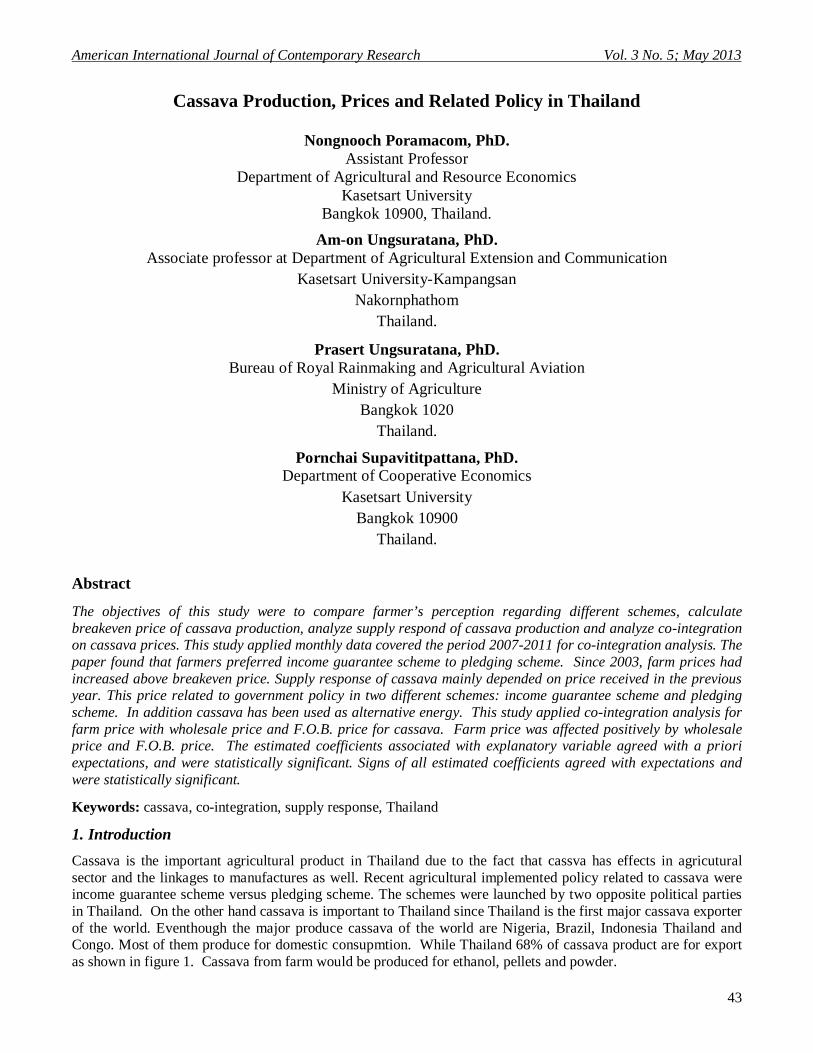
Cassava is the important agricultural product in Thailand due to the fact that cassva has effects in agricutural sector and the linkages to manufactures as well. Recent agricultural implemented policy related to cassava were income guarantee scheme versus pledging scheme. The schemes were launched by two opposite political parties in Thailand. On the other hand cassava is important to Thailand since Thailand is the first major cassava exporter of the world. Eventhough the major produce cassava of the world are Nigeria, Brazil, Indonesia Thailand and Congo. Most of them produce for domestic consupmtion. While Thailand 68% of cassava product are for export as shown in figure 1. Cassava from farm would be produced for ethanol, pellets and powder.
© Center for Promoting Ideas, USA www.aijcrnet.com
44
They composed of 5% as ethanol, 8% pellets for domestic consumption, 32% pellets for export, 19% powder for domestic consumption and 36% powder for export.
Source: Thai Tapioca Starch Association Figure 1: flow of source and use of cassava and products in Thailand
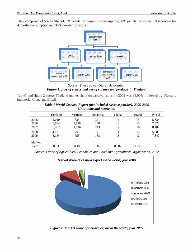
Table1 and figure 2 shows Thailand market share on cassava export in 2009 was 83.00%, followed by Vietnam, Indonesia, China and Brazil.
Table 1 World Cassava Export (not included cassava powder), 2005-2009 Unit: thousand metric ton
Thailand Vietnam Indonesia China Brazil World
2005 4,040 534 341 16 15 5,634 2006 5,884 1,040 148 16 15 7,378 2007 5,962 1,316 243 17 16 8,107 2008 4,121 753 171 14 13 5,589 2009 6,154 753 183 18 12 7,340
Market share 0.83 0.10 0.02 0.002 0.001 1
Source: Office of Agricultural Economics and Food and Agricultural Organization, 2012
Figure 2: Market share of cassava export in the world, year 2009
cassava from farm
pellet
domestic consumption 8% export 32%
ethanol 5% powder
domestic consumption
19%export 36%
Market share of cassava export in the world, year 2009
Thailand 0.83
Vietnam 0.10
Indonesia 0.02
China 0.002
Brazil 0.001
American International Journal of Contemporary Research Vol. 3 No. 5; May 2013
45
Literature Review
As importance of cassava to Thailand, this study emphasized 2 main components: supply response of cassava and co-integration of cassava prices. There were several literatures related to these topics. Salassi(1995) addressed a supply response model of supply-inducing price, lagged planted acreage, expected variable cash production cost as independent variables. Chowdhury and Herndon (2000) developed a supply response model for rice-growing state using policy-inducing variable. The single equation regression model for each rice-producing state is estimated by using the ordinary least square method. The estimated parameter shows a significant inverse relationship between the rice acreage planted and policy-inducing prices in all of the rice-growing states. Kuwornu et.al (2011) developed supply response model of rice in Ghana: a co-integration analysis over the period 1970-2008. Annual time series data of aggregated output, total land area cultivated, yield, real prices of rice and maize, and rainfall were used for the analysis. The Augmented-Dickey Fuller test was used to estimate the short run and long run elasticities. On the other hand, FAO (2005) aimed to provide the evidence on price transmission in a number of agricultural markets for sixteen countries, including Thailand, primarily for basic food commodities. Both spatial and vertical price relation are considered, as the data base includes prices at the producer, wholesale and retail levels. Kamokar et al. (2011) used multico-integration analysis on rice in 6 districts in Bangaladesh. They found co-integration in two districts with the long run speed of adjustment coefficient of 66%. They also applied Granger causality approach. This study follows Salassi supply response model, using annual data 2002-2010. Similar to FAO and Karmokar studies, this study applied monthly data covered the period 2007-2011 for co-integration analysis.
Objectives
The objectives of this study were to:
1) compare farmer’s perception regarding different schemes 2) calculate breakeven price of cassava production 3) analyze supply respond of cassava production 4) analyze co-integration on cassava prices
2. Methodology
Data
The primary data on farmers’ perception regarding two different rice schemes. The research interviewed farmers in Nakornratchasima province. Secondary data were used for break even analysis, supply respond and co-integration analysis on prices. Monthly data on farm price, wholesale price and F.O.B. prices are used in the analysis. The data covered the period 2007- 2011. Prices are expressed in current terms on a common unit basis of 1,000 kilogram. The data are taken from various issues and web sites of Department of Agricultural Economics, Department of Interior Trade of Thailand and Department of Custom of Thailand.
Analysis
The research would compare farmer’s perception regarding to different schemes: income guarantee scheme and pledging scheme. Income guarantee scheme performance of cassava in Thailand during 2009-2011 was shown.
1. Cassava break-even analysis
P = cassava farm price (USD/ton)
Q = cassava yield (ton/acre)
F = cassava fixed cost (USD/ton)
V = cassava variable cost (USD/ton)
(P X Q)=F + (V X Q)
P =(F/Q)+V
© Center for Promoting Ideas, USA www.aijcrnet.com
46
2. Cassava supply respond model
),,,( 1 DCPAfA titt
tA cassava cultivated area in recent year itA cassava cultivated area in the previous year
1tP = cassava farm rice price in the previous year
C = cassava cost per area D = cassava pledging scheme or income guarantee scheme
3. Co-integration analysis
The study estimated cassava price transmission from different levels using unit root and co-integration methods. Market co-integration involves a test of price efficiency by examining how market in different regions responds jointly to supply and demand forces. Each cassava price series are tested for the order of integration to determine which variables are stationary and non-stationary in levels. The Augmented Dickey and Fuller test (ADF) developed by Dickey and Fuller (1979 and 1981) was used for a unit root test for all variables. The null hypothesis of a unit root is rejected if variable is stationary. To elaborate a long-term relationship between cassava farm price and cassava wholesale price and cassava F.O.B. price, the two step procedure of Engle and Granger (1987) was employed. First a simple linear model is estimated using ordinary least square and then the residues were tested for stationary. Then the Johansen co-integration test, based on the Dickey-Fuller procedure, determines the number of co-integration equation. Co-integration methods are useful when time series data are non-stationary and conventional model would encounter the problem of spurious regression (Harris, 1995)
Long run co-integration
푃 = 훼푖 + β푖푃 + 푒
푃 = α푖 + β푖푃 + 푒
Short run co-integration
∆푃 = a + δ푖∆푃 + 훾푖휀 ∆푃 = b + δ푖∆푃 + 훾푖휀
3. Results and Discussion
By interview 103 farmers in Sungsang district, Nakornratchasima province-in the Northeastern region, 83.50% of farmers grow cassava, depending on rain. Farmers grow cassava once a year for 12 month period. 49.51% of farmers received the loan from Bank for Agriculture and Agricultural Cooperatives (BAAC). In 2009/2010, farmers sold cassava at the average of baht 2,750 per metric ton. They received the difference price compensation for baht 582.62 per metric ton (total of USD18.20). Farmers preferred income guarantee scheme to pledging scheme at 84.31%. Due to the reason that income guarantee scheme had fewer procedures than pledging scheme. Farmers could sell their product at any price level when they wanted.
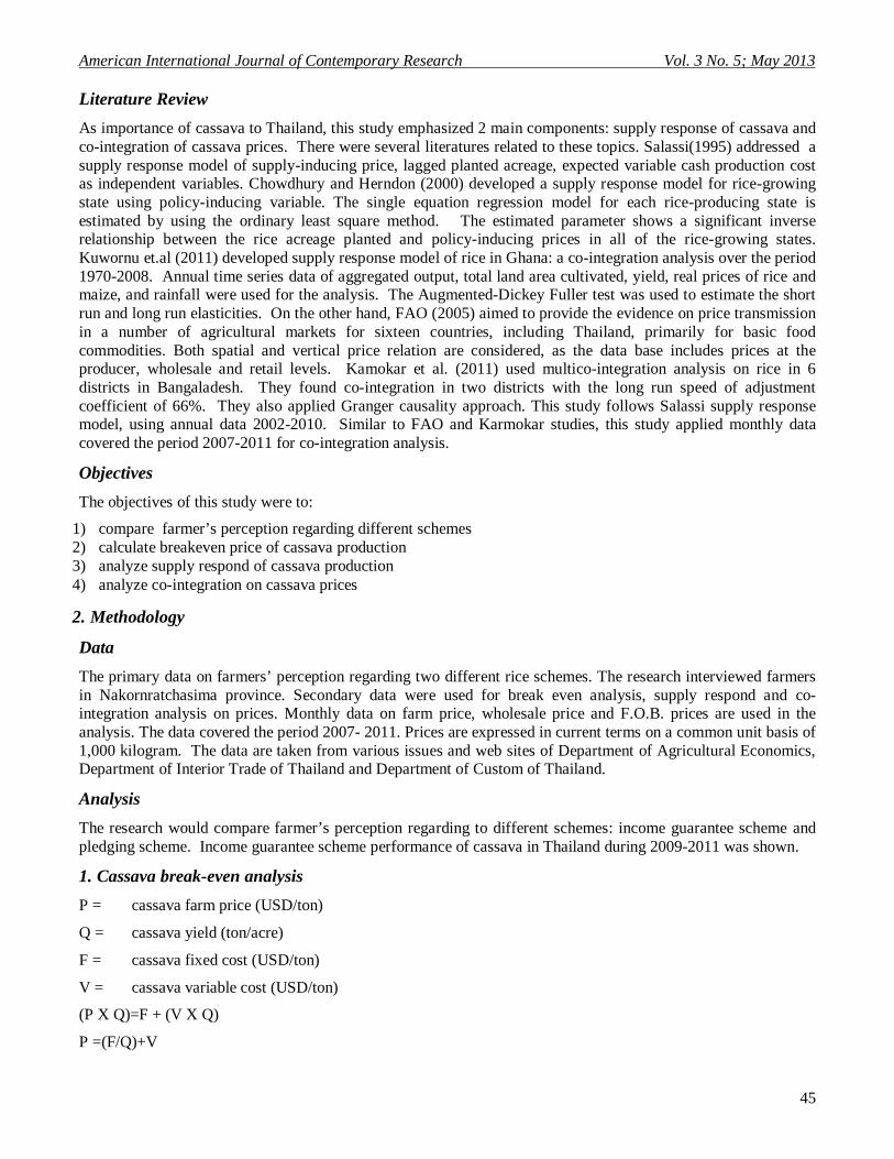
In addition after register as growers they could receive the difference even when the crop was lost by disease or flood. Table 2 shows the performance of income guarantee scheme for cassava in Thailand during 2010-2011. Total cassava farmers involved in Income Guarantee policy during 2010-2011 were 391,000 farmers and there were the maximum 247,000 farmers in the northeast of Thailand. Total government budget used for the policy was USD million 78.48 and each farmer received the payment approximately USD206.26.
American International Journal of Contemporary Research Vol. 3 No. 5; May 2013
47
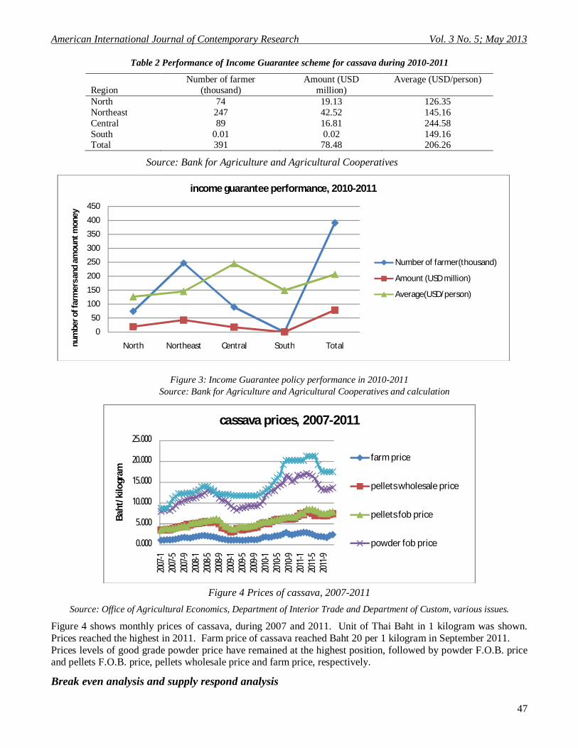
Table 2 Performance of Income Guarantee scheme for cassava during 2010-2011
Region Number of farmer
(thousand) Amount (USD
million) Average (USD/person)
North 74 19.13 126.35 Northeast 247 42.52 145.16 Central 89 16.81 244.58 South 0.01 0.02 149.16 Total 391 78.48 206.26
Source: Bank for Agriculture and Agricultural Cooperatives
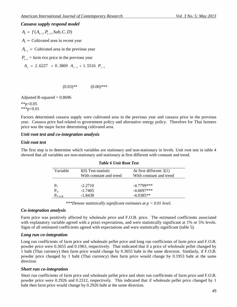
Figure 3: Income Guarantee policy performance in 2010-2011
Source: Bank for Agriculture and Agricultural Cooperatives and calculation
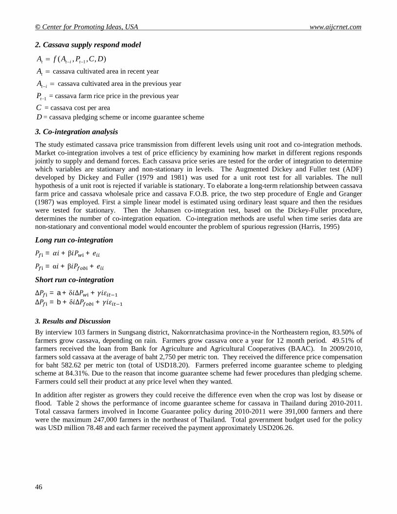
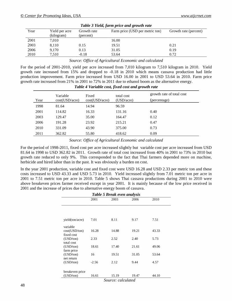
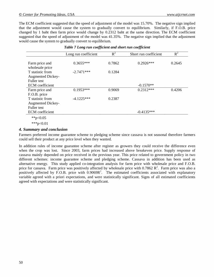
Figure 4 Prices of cassava, 2007-2011
Source: Office of Agricultural Economics, Department of Interior Trade and Department of Custom, various issues.
Figure 4 shows monthly prices of cassava, during 2007 and 2011. Unit of Thai Baht in 1 kilogram was shown. Prices reached the highest in 2011. Farm price of cassava reached Baht 20 per 1 kilogram in September 2011. Prices levels of good grade powder price have remained at the highest position, followed by powder F.O.B. price and pellets F.O.B. price, pellets wholesale price and farm price, respectively.
Break even analysis and supply respond analysis
0
50
100
150
200
250
300
350
400
450
North Northeast Central South Totalnum
ber o
f far
mer
s and
am
ount
mon
ey
income guarantee performance, 2010-2011
Number of farmer(thousand)
Amount (USD million)
Average(USD/person)
0.000
5.000
10.000
15.000
20.000
25.000
2007
-1
2007
-5
2007
-9
2008
-1
2008
-5
2008
-9
2009
-1
2009
-5
2009
-9
2010
-1
2010
-5
2010
-9
2011
-1
2011
-5
2011
-9
Baht
/kilo
gram
cassava prices, 2007-2011
farm price
pellets wholesale price
pellets fob price
powder fob price
© Center for Promoting Ideas, USA www.aijcrnet.com
48
Table 3 Yield, farm price and growth rate
Year Yield per acre (kilogram)
Growth rate (percent)
Farm price (USD per metric ton) Growth rate (percent)
2001 7,010 16.00 2003 8,110 0.15 19.51 0.21 2006 9,170 0.13 31.05 0.19 2010 7,510 -0.18 53.64 0.72
Source: Office of Agricultural Economic and calculated
For the period of 2001-2010, yield per acre increased from 7,010 kilogram to 7,510 kilogram in 2010. Yield growth rate increased from 15% and dropped to -0.18 in 2010 which means cassava production had little production improvement. Farm price increased from USD 16.00 in 2001 to USD 53.64 in 2010. Farm price growth rate increased from 21% in 2001 to 72% in 2011 due to ethanol boom as the alternative energy.
Table 4 Variable cost, fixed cost and growth rate
Year Variable cost(USD/acre)
Fixed cost(USD/acre)
total cost (USD/acre)
growth rate of total cost (percentage)
1998 81.64 14.94 96.59 2001 114.82 16.33 131.16 0.40
2003 129.47 35.00 164.47 0.12 2006 191.28 23.92 215.21 0.47 2010 331.09 43.90 375.00 0.73 2011 362.82 55.80 418.62 0.09
Source: Office of Agricultural Economic and calculated
For the period of 1998-2011, fixed cost per acre increased slightly but variable cost per acre increased from USD 81.64 in 1998 to USD 362.82 in 2011. Growth rate of total cost increased from 40% in 2001 to 73% in 2010 but growth rate reduced to only 9%. This corresponded to the fact that Thai farmers depended more on machine, herbicide and hired labor than in the past. It was obviously a burden on cost.
In the year 2001 production, variable cost and fixed cost were USD 16.28 and USD 2.33 per metric ton and these costs increased to USD 43.33 and USD 5.73 in 2010. Yield increased slightly from 7.01 metric ton per acre in 2001 to 7.51 metric ton per acre in 2010. Table 5 shows Thai cassava productions during 2001 to 2010 were above breakeven prices farmer received except in year 2001. It is mainly because of the low price received in 2001 and the increase of prices due to alternative energy boom of cassava.
Table 5 Break even analysis
2001
2003
2006
2010
yield(ton/acre) 7.01 8.11 9.17 7.51
variable cost(USD/ton)
16.28 14.88 19.21 43.33
fixed cost (USD/ton) 2.33 2.52 2.40 5.73 total cost (USD/ton) 18.61 17.40 21.61 49.06 farm price (USD/ton) 16 19.51 31.05 53.64 net return (USD/ton) -2.56 2.12 9.44 4.57 breakeven price (USD/ton) 16.61 15.19 19.47 44.10
Source: calculated
American International Journal of Contemporary Research Vol. 3 No. 5; May 2013
49
Cassava supply respond model
),,,,( 1 DCSubPAfA titt
tA Cultivated area in recent year itA Cultivated area in the previous year
1tP = farm rice price in the previous year
11 5516.13869.06227.2 ttt PAA
(0.03)** (0.00)***
Adjusted R-squared = 0.8696 **p<0.05 ***p<0.01
Factors determined cassava supply were cultivated area in the previous year and cassava price in the previous year. Cassava price had related to government policy and alternative energy policy. Therefore for Thai farmers price was the major factor determining cultivated area.
Unit root test and co-integration analysis
Unit root test
The first step is to determine which variables are stationary and non-stationary in levels. Unit root test in table 4 showed that all variables are non-stationary and stationary at first different with constant and trend.
Table 6 Unit Root Test
Variable I(0) Test-statistic With constant and trend
At first different: I(1) With constant and trend
Pf -2.2710 -4.7799*** Pw -1.7405 -4.6697*** PF.O.B. -1.8438 -4.0385**
***Denote statistically significant estimates at p < 0.01 level.
Co-integration analysis
Farm price was positively affected by wholesale price and F.O.B. price. The estimated coefficients associated with explanatory variable agreed with a priori expectations, and were statistically significant at 1% or 5% levels. Signs of all estimated coefficients agreed with expectations and were statistically significant (table 5).
Long run co-integration
Long run coefficients of farm price and wholesale pellet price and long run coefficients of farm price and F.O.B. powder price were 0.3655 and 0.1963, respectively. That indicated that if a price of wholesale pellet changed by 1 baht (Thai currency) then farm price would change by 0.3655 baht in the same direction. Similarly, if F.O.B. powder price changed by 1 baht (Thai currency) then farm price would change by 0.1953 baht at the same direction
Short run co-integration
Short run coefficients of farm price and wholesale pellet price and short run coefficients of farm price and F.O.B. powder price were 0.2926 and 0.2312, respectively. This indicated that if wholesale pellet price changed by 1 baht then farm price would change by 0.2926 baht at the same direction.
© Center for Promoting Ideas, USA www.aijcrnet.com
50
The ECM coefficient suggested that the speed of adjustment of the model was 15.70%. The negative sign implied that the adjustment would cause the system to gradually convert to equilibrium. Similarly, if F.O.B. price changed by 1 baht then farm price would change by 0.2312 baht at the same direction. The ECM coefficient suggested that the speed of adjustment of the model was 41.35%. The negative sign implied that the adjustment would cause the system to gradually convert to equilibrium.
Table 7 Long run coefficient and short run coefficient
Long run coefficient R2 Short run coefficient R2 Farm price and wholesale price
0.3655*** 0.7862 0.2926***
0.2645
T statistic from Augmented Dickey-Fuller test
-2.7471*** 0.1284
ECM coefficient -0.1570** Farm price and F.O.B. price
0.1953*** 0.9069 0.2312*** 0.4206
T statistic from Augmented Dickey-Fuller test
-4.1225*** 0.2387
ECM coefficient -0.4135***
**p<0.05
***p<0.01
4. Summary and conclusion
Farmers preferred income guarantee scheme to pledging scheme since cassava is not seasonal therefore farmers could sell their product at any price level when they wanted.
In addition rules of income guarantee scheme after register as growers they could receive the difference even when the crop was lost. Since 2003, farm prices had increased above breakeven price. Supply response of cassava mainly depended on price received in the previous year. This price related to government policy in two different schemes: income guarantee scheme and pledging scheme. Cassava in addition has been used as alternative energy. This study applied co-integration analysis for farm price with wholesale price and F.O.B. price for cassava. Farm price was positively affected by wholesale price with 0.7862 R2. Farm price was also a positively affected by F.O.B. price with 0.9069R2. The estimated coefficients associated with explanatory variable agreed with a priori expectations, and were statistically significant. Signs of all estimated coefficients agreed with expectations and were statistically significant.
American International Journal of Contemporary Research Vol. 3 No. 5; May 2013
51
References
Bank for Agriculture and Agricultural Cooperatives. 2011. Performance of Income guarantee scheme for cassava during 2010-2011. Unpublished document.
Chowdhury A.A. Farhad and Cary W. Herdon, JR. 2000. “Supply Response of Farm Program in Rice-growing States.” International Advances in Economics Research 6(November): 771-781.
Department of Custom. 2012. Export values and quantity of cassava. Department of Interior Trade. 2012. Wholesale prices of cassava. www.dit.go.th accessed in March 2012. Dickey, D.A., and W.A. Fuller. 1979. “Distribution of the Estimators for Autoregressive Time Series with a Unit
Root.” Journal of the American Statistical Association 74(June): 427-431. Dickey, D.A. and W.A. Fuller. 1981. “Likelihood Ratio Statistics for Autoregressive Time Series with a Unit
Root.” Econometrica 49(July): 1057-1072. Engle, R.F. and D.W.J. Granger. 1987. “Co-Integration and Error Correction: Representation, Estimation and
Testing.” Econometrica 55(March): 251-276. Food and Agriculture Organization, 2005. “Price Transmission in Selected Agricultural Markets.” Harris, R.I.D. 1995. Using Cointegration Analysis in Econometric Modeling. Edinburgh Gate: Prentice-Hall. Karmokar Kumar Provash, Mahendran Shitan and A.B. M. Alam Beg. 2011. “Mutico-integration Analysis on the
High Yield Boro Rice of Six Slected Districts in Bangladesh.” African Journal of Agricultural Research 6(September):4654-4660.
Kuwornu John K.M., Mannikuu P.M.Izideen and Yaw B. Osei-Asare. 2011. “Supply Response of Rice in Ghana: A Co-integration Analysis.” Journal of Economics and Sustainable Development 2(October):1-13.
Office of Agricultural Economics. 2011. Agricultural Statistics of Thailand 2010. http://www.doae.go.th/ . Salassi M.E. 1995. “The Responsiveness of U.S. Rice Acreagre to Price and Production Costs.” Journal of Agricultural and Applied Economics 27(December): 386-399. http://www.mfa.go.th
Recommended