Download pdf - Capital Gains and Inequality of Personal Income: Some Results from Survey Data

Capital Gains and Inequality of Personal Income: Some Results from Survey DataAuthor(s): Kul B. BhatiaSource: Journal of the American Statistical Association, Vol. 71, No. 355 (Sep., 1976), pp. 575-580Published by: American Statistical AssociationStable URL: http://www.jstor.org/stable/2285585 .

Accessed: 15/06/2014 11:29

Your use of the JSTOR archive indicates your acceptance of the Terms & Conditions of Use, available at .http://www.jstor.org/page/info/about/policies/terms.jsp

.JSTOR is a not-for-profit service that helps scholars, researchers, and students discover, use, and build upon a wide range ofcontent in a trusted digital archive. We use information technology and tools to increase productivity and facilitate new formsof scholarship. For more information about JSTOR, please contact [email protected].

.

American Statistical Association is collaborating with JSTOR to digitize, preserve and extend access to Journalof the American Statistical Association.

http://www.jstor.org

This content downloaded from 91.229.248.154 on Sun, 15 Jun 2014 11:29:51 AMAll use subject to JSTOR Terms and Conditions

http://www.jstor.org/action/showPublisher?publisherCode=astata

http://www.jstor.org/stable/2285585?origin=JSTOR-pdf

http://www.jstor.org/page/info/about/policies/terms.jsp


Capital Gains and Inequality of Personal Income: Some Results from Survey Data

KUL B. BHATIA*

This paper deals with income distribution of capital gains and their effect on measures of income inequality for 1962. Aggregate accrued gains are allocated to various income classes by using microdata from the Survey of Financial Characteristics of Consumers. The results show that accrued gains are distributed more unevenly than money income. The Gini coefficient drops from 0.41 to 0.35 when accrued losses for 1962 are subtracted from income, but it increases to 0.43 when average gains for 1960-64 are added to income. Variance of natural logarithms, the other measure of inequality used, also shows a similar pattern.

1. INTRODUCTION

The objective of this study is to estimate the income distribution of accrued capital gains and determine how the inclusion of capital gains in income will alter the distribution of personal income and the commonly used measures of income inequality in the United States. Be- tween 1948 and 1964, capital gains accrued at an average rate of over $40 billion a year on corporate stock, real estate, and farm assets owned by individuals, who, on an average, reported about $9 billion of realized gains every year for income tax purposes during this period. Data on gains realized by people in various income brackets published in Statistics of Income [17] were incorporated into personal income by Liebenberg and Fitzwilliams [10] for 1958, but little information is available on the distribution of accrued gains, although it is widely be- lieved that gains accrue mostly to upper income groups. Arena [2] and Granger and Mlorgenstern [8] even use this argument to explain why accrued gains will not affect aggregate consumption or other economic magnitudes.

Whether capital gains are a component of income has been the subject of a longstanding controversy among income theorists. Most well-known studies of the size distribution of personal income, for example, by Gold- smith [7], Miller [12], and Schultz [16], do not include accrued capital gELins, nor are gains incorporated in national accounts or the official measures of personal income (compiled by BEA, the Bureau of Economic Analy- sis). Although there are several theoretical reasons for including accrued capital gains in national income, a case for including them in personal income can be based simply on the argument that accrued gains enhance the

* Kul B. Bhatia is Assistant Professor, Department of Economics, University of Western Ontario, London, Ontario, Canada N6A 5C2. This research was supported by a grant from the Canada Council. The author wishes to thank Michael B. McElroy and Peter J. Kuch for helpful comments on an earlier draft, and I. Tapley and J. Johnson for their competent programming. He also would like to thank the referee for helpful suggestions.

purchasing power of an individual. They can be spent or saved almost like any other type of income; therefore, an income concept broader than the OBE measure will be a better indicator of the true change in the economic position of the personal sector.'

The failure to include capital gains in income has many implications for personal income, its size distribution, and the whole area of personal income taxation.

1. Aggregate personal income as reported and saving estimated from it do not correctly represent the economic position of individuals or their saving.2

2. By including only a portion of realized gains in the tax base, a very profitable loophole for converting income into capital gains, has been provided to those who can, and the profit- ability increases directly with the marginal tax rate.3

3. Most important for the concerns of this paper, the existing knowledge about the inequality of the size distribution of income is probably incorrect.'

The plan of the paper is as follows. Section 2 presents a brief review of the present state of knowledge about realized and accrued gains and their distribution by income brackets; accrued gains are allocated to income classes in Section 3; effects on measures of income inequality for 1962 are discussed in Section 4; and Section 5 concludes with a critical summary of these results. Most of the results reported here have been derived from the original data collected for the Survey of Financial Charac- teristics of Consumers (SFCC).

I For a discussion of the debate on including capital gains in national income, see [3, 11]. The inclusion of accrued gains in personal income is one step toward the all-inclusive Haig-Hicks-Simon concept of income which, roughly, defines income as the maximum amount that can be spent while keeping net worth constant.

2 Bhatia [3] showed that when accrued gains were added to personal income, the official estimates of both personal income and saving changed considerably and showed much greater cyclical variability than before.

IThere is no tax on accrued gains, and the maximum rate of tax on realized gains is one-half the marginal rate of tax, subject to an upper limit. Thus, anyone who can convert income into gains can reduce his tax liability considerably. Tax aspects of this problem, however, require different definitions and data from those employed here, e.g., adjusted gross income instead of money income, incomes of individuals and couples, not family income. These matters are dealt with in a separate paper (see [4]).

4 For example, data reported by Schultz [16, p. 79] from Current Population Survey, shows that the Gini coefficient of income of families and unrelated individuals in the U.S. has varied between 0.4 and 0.43 during the period 1947-1965, except in 1955 when it was 0.45. Also, Brimmer [5, p. 41] states that the distribution of personal income has continued to move toward greater equality in recent years. McElroy [11] found that the Gini coefficient for accrued gains varied between 0.6 and 0.7 in some years during this period. Thus, if gains are included in income, the resulting distribution will be more unequal than the official statistics indicate, and the degree of inequality will also be more variable.

O Journal of the American Statistical Association September 1976, Volume 71, Number 355

Applications Section

575



576 Journal of the American Statistical Association, September 1976

2. BELIEFS VERSUS FACTS

Liebenberg and Fitzwilliams [10], working with a sample of income tax returns, examined the effects of realized gains on income distribution at length for 1958. They found that capital gains were widely dispersed, and both average gains and the percent of units realizing gains rose with income level. They classified all units by money income and money income plus realized gains.' The latter classification caused an upward shift of units to higher income classes-the number increased by almost 7 percent in income brackets above $25,000-but realized gains, being only 24 percent of family personal income, were too small to alter the distribution of personal income radically.

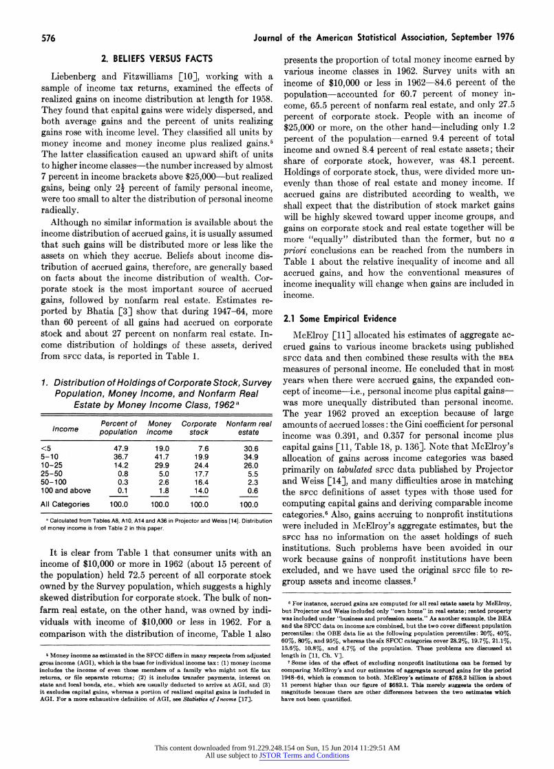
Although no similar information is available about the income distribution of accrued gains, it is usually assumed that such gains will be distributed more or less like the assets on which they accrue. Beliefs about income distribution of accrued gains, therefore, are generally based on facts about the income distribution of wealth. Cor- porate stock is the most important source of accrued gains, followed by nonfarm real estate. Estimates reported by Bhatia [3] show that during 1947-64, more than 60 percent of all gains had accrued on corporate stock and about 27 percent on nonfarm real estate. In- come distribution of holdings of these assets, derived from SFCC data, is reported in Table 1.

1. Distribution of Holdings of Corporate Stock, Survey Population, Money Income, and Nonfarm Real

Estate by Money Income Class, 1962a

Percent of Money Corporate Nonfarm real Income population income stock estate

<5 47.9 19.0 7.6 30.6 5-10 36.7 41.7 19.9 34.9 10-25 14.2 29.9 24.4 26.0 25-50 0.8 5.0 17.7 5.5 50-100 0.3 2.6 16.4 2.3 100 and above 0.1 1.8 14.0 0.6

All Categories 100.0 100.0 100.0 100.0

a Calculated from Tables A8, A10, A14 and A36 in Projector and Weiss [141. Distribution of money income is from Table 2 in this paper.

It is clear from Table 1 that consumer units with an income of $10,000 or more in 1962 (about 15 percent of the population) held 72.5 percent of all corporate stock owned by the Survey population, which suggests a highly skewed distribution for corporate stock. The bulk of nonfarm real estate, on the other hand, was owned by individuals with income of $10,000 or less in 1962. For a comparison with the distribution of income, Table l also

5 Money income as estimated in the SFCC differs in many respects from adjusted gross income (AGI), which is the base for individual income tax: (1) money income includes the income of even those members of a family who might not file tax returns, or file separate returns; (2) it includes transfer payments, interest on state and local bonds, etc., which are usually deducted to arrive at AGI, and (3) it excludes capital gains, whereas a portion of realized capital gains is included in AGI. For a more exhaustive definition of AGI, see Statistics of Income ?17].

presents the proportion of total money income earned by various income classes in 1962. Survey units with an income of $10,000 or less in 1962-84.6 percent of the population-accounted for 60.7 percent of money income, 65.5 percent of nonfarm real estate, and only 27.5 percent of corporate stock. People with an income of $25,000 or more, on the other hand-including only 1.2 percent of the population-earned 9.4 percent of total income and owned 8.4 percent of real estate assets; their share of corporate stock, however, was 48.1 percent. Holdings of corporate stock, thus, were divided more unevenly than those of real estate and money income. If accrued gains are distributed according to wealth, we shall expect that the distribution of stock market gains will be highly skewed toward upper income groups, and gains on corporate stock and real estate together will be more "equally" distributed than the former, but no a priori conclusions can be reached from the numbers in Table 1 about the relative inequality of income and all accrued gains, and how the conventional measures of income inequality will change when gains are included in income.

2.1 Some Empirical Evidence

McElroy [11] allocated his estimates of aggregate accrued gains to various income brackets using published SFCc data and then combined these results with the BEA

measures of personal income. He concluded that in most years when there were accrued gains, the expanded concept of income-i.e., personal income plus capital gains- was more unequally distributed than personal income. The year 1962 proved an exception because of large amounts of accrued losses: the Gini coefficient for personal income was 0.391, and 0.357 for personal income plus capital gains [11, Table 18, p. 136]. Note that McElroy's allocation of gains across income categories was based primarily on tabulated SFcc data published by Projector and Weiss [14], and many difficulties arose in matching the SFCc definitions of asset types with those used for computing capital gains and deriving comparable income categories.6 Also, gains accruing to nonprofit institutions were included in iAJcElroy's aggregate estimates, but the SFCC has no information on the asset holdings of such institutions. Such problems have been avoided in our work because gains of nonprofit institutions have been excluded, and we have used the original SFCC file to re- group assets and income classes.7

6 For instance, accrued gains are computed for all real estate assets by McElroy, but Projector and Weiss included only "own home" in real estate; rented property was included under "business and profession assets." As another example, the BEA and the SFCC data on income are combined, but the two cover different population percentiles: the OBE data lie at the following population percentiles: 20%, 40%, 60%, 80%, and 95%, whereas the six SFCC categories cover 28.2%, 19.7%, 21.1%, 15.6%, 10.8%, and 4.7% of the population. These problems are discussed at length in [11, Ch. V].

7 Some idea of the effect of excluding nonprofit institutions can be formed by comparing McElroy's and our estimates of aggregate accrued gains for the period 1948-64, which is common to both. McElroy's estimate of $768.2 billion is about 11 percent higher than our figure of $682.1. This merely suggests the orders of magnitude because there are other differences between the two estimates which have not been quantified.



Capital Gains and Income-inequality 577

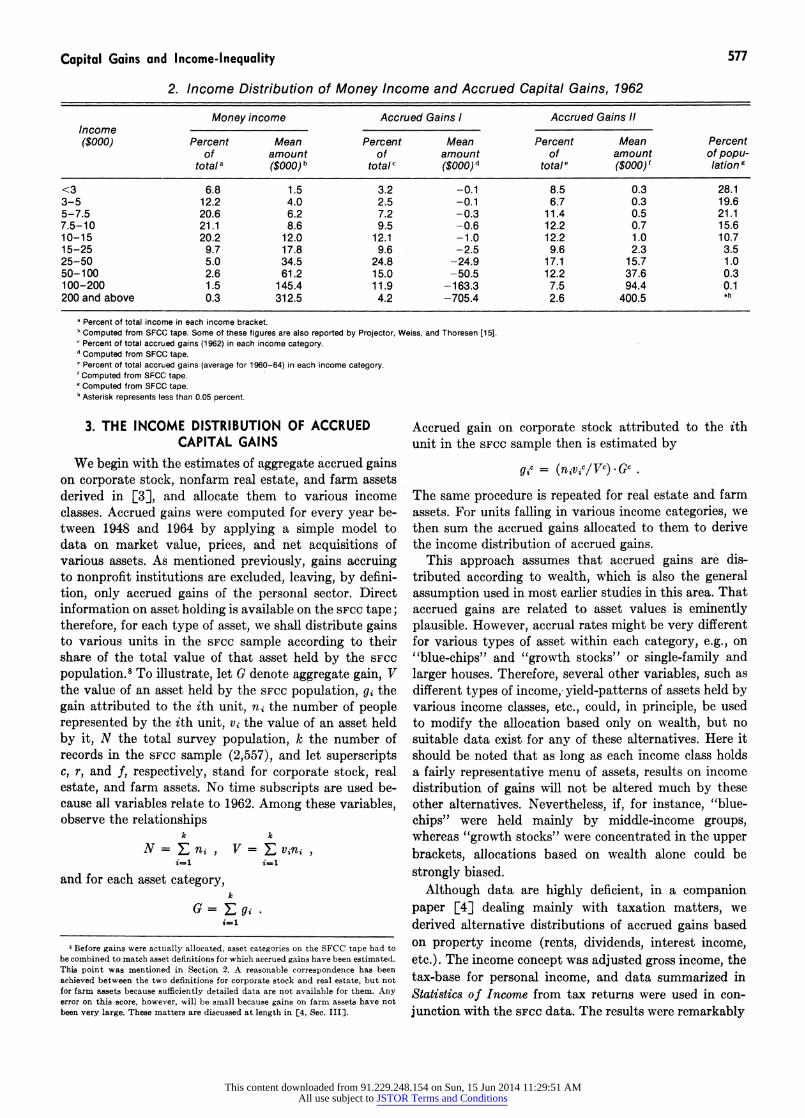
2. Income Distribution of Money Income and Accrued Capital Gains, 1962

Money income Accrued Gains I Accrued Gains I1 Income ($000) Percent Mean Percent Mean Percent Mean Percent

of amount of amount of amount of popu- totala ($000)b totalc ($000)d totale ($000), lation

<3 6.8 1.5 3.2 -0.1 8.5 0.3 28.1 3-5 12.2 4.0 2.5 -0.1 6.7 0.3 19.6 5-7.5 20.6 6.2 7.2 -0.3 11.4 0.5 21.1 7.5-10 21.1 8.6 9.5 -0.6 12.2 0.7 15.6 10-15 20.2 12.0 12.1 -1.0 12.2 1.0 10.7 15-25 9.7 17.8 9.6 -2.5 9.6 2.3 3.5 25-50 5.0 34.5 24.8 -24.9 17.1 15.7 1.0 50-100 2.6 61.2 15.0 -50.5 12.2 37.6 0.3 100-200 1.5 145.4 11.9 -163.3 7.5 94.4 0.1 200 and above 0.3 312.5 4.2 -705.4 2.6 400.5 *h

Percent of total income in each income bracket. Computed from SFCC tape. Some of these figures are also reported by Projector, Weiss, and Thoresen [151. Percent of total accrued gains (1962) in each income category.

dComputed from SFCC tape. e Percent of total accrued gains (average for 1960-64) in each income category. Computed from SFCC tape.

'Computed from SFCC tape. Asterisk represents less than 0.05 percent.

3. THE INCOME DISTRIBUTION OF ACCRUED CAPITAL GAINS

We begin with the estimates of aggregate accrued gains on corporate stock, nonfarm real estate, and farm assets derived in [3], and allocate them to various income classes. Accrued gains were computed for every year between 1948 and 1964 by applying a simple model to data on market value, prices, and net acquisitions of various assets. As mentioned previously, gains accruing to nonprofit institutions are excluded, leaving, by definition, only accrued gains of the personal sector. Direct information on asset holding is available on the sFcc tape; therefore, for each type of asset, we shall distribute gains to various units in the SFCC sample according to their share of the total value of that asset held by the SFCC population.8 To illustrate, let G denote aggregate gain, V the value of an asset held by the SFCC population, gi the gain attributed to the ith unit, ni the number of people represented by the ith unit, vi the value of an asset held by it, N the total survey population, k the number of records in the SFCC sample (2,557), and let superscripts c, r, and f, respectively, stand for corporate stock, real estate, and farm assets. No time subscripts are used because all variables relate to 1962. Among these variables, observe the relationships

k k

N ni , V vni i=1 i=l

and for each asset category, k

G= Eg. i-i

a Before gains were actually allocated, asset categories on the SFCC tape had to be combined to match asset definitions for which accrued gains have been estimated. This point was mentioned in Section 2. A reasonable correspondence has been achieved between the two definitions for corporate stock and real estate, but not for farm assets because sufficiently detailed data are not available for them, Any error on this score, however, will be small because gains on farm assets have not been very large. These matters are discussed at length in [4, Sec. III].

Accrued gain on corporate stock attributed to the ith unit in the SFCC sample then is estimated by

gic = (niv,c/Vc).Gc

The same procedure is repeated for real estate and farm assets. For units falling in various income categories, we then sum the accrued gains allocated to them to derive the income distribution of accrued gains.

This approach assumes that accrued gains are distributed according to wealth, which is also the general assumption used in most earlier studies in this area. That accrued gains are related to asset values is eminently plausible. However, accrual rates might be very different for various types of asset within each category, e.g., on "blue-chips" and "growth stocks" or single-family and larger houses. Therefore, several other variables, such as different types of income, yield-patterns of assets held by various income classes, etc., could, in principle, be used to modify the allocation based only on wealth, but no suitable data exist for any of these alternatives. Here it should be noted that as long as each income class holds a fairly representative menu of assets, results on income distribution of gains will not be altered much by these other alternatives. Nevertheless, if, for instance, "blue- chips" were held mainly by middle-income groups, whereas "growth stocks" were concentrated in the upper brackets, allocations based on wealth alone could be strongly biased.

Although data are highly deficient, in a companion paper [4] dealing mainly with taxation matters, we derived alternative distributions of accrued gains based on property income (rents, dividends, interest income, etc.). The income concept was adjusted gross income, the tax-base for personal income, and data summarized in Statistics of Income from tax returns were used in con- junction with the SFCC data. The results were remarkably




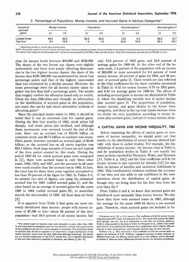
3. Percentage of Population, Money Income, and Accrued Gains in Various Categories a

Income & Money income Population Accrued gains I Accrued gains It accrued -_-_-

gain.s Wi (jJ) fi (i)()(i)()Wi

Lowest three 39.6 36.0 68.8 65.5 12.9 6.3 26.6 16.7 Top four 9.4 10.9 1.4 1.9 55.9 70.9 39.4 50.7

a Classifying variable is income plus accrued gains. NOTE: All columns marked (i) are from Table 2, and use money income as classifying variable. Columns marked (ii) are based on money income plusaccrued gainsas classifying variable. The lowest three categories include people with income plus accrued gains of $7,500 or less, and the top four, those with income plus accrued gains of $25,000 or more.

close for income levels between $10,000 and $100,000. The shares of the two lowest AGI classes were slightly understated, and there were nearly offsetting discrepan- cies in the two highest income classes: the share of the income class $100-200,000 was understated by about four percentage points and that of the highest, open-ended class was overstated by a similar amount. However, the mean percentage error for all income classes taken together was less than half a percentage point. The results thus roughly confirm the allocation based only on wealth. Given the data difficulties and virtually no information on the distribution of accrued gains in the population, not much else can be said about alternative methods of allocating gains.9

Since the principal results relate to 1962, it should be noted that it was an abnormal year for capital gains. During the first four months of 1962, stock prices fell sharply, real estate prices also declined, and although these movements were reversed toward the end of the year, there was an accrued loss of $52.95 billion on corporate stock, and $6.75 billion on nonfarm real estate. Farm assets, however, recorded an accrued gain of $6.64 billion; so the accrued loss on all assets together was $53.1 billion. Such large amounts of losses are not typical of the time period covered by this study. During the period 1947-64 for which accrued gains were computed in [3], there were accrued losses in only three other years, 1949, 1953, and 1957, and the amounts in all cases were much smaller than the accrued loss in 1962. In fact, the total loss for these three years together amounted to less than 70 percent of the figure for 1962. In Tables 2-5, we present two sets of figures, one using the estimated accrued loss for 1962 (called accrued gains I), and the other based on an average of accrued gains for the years 1960 to 1964 (called accrued gains II), to somewhat smooth the abnormality of 1962. All these data are from [3].

It is apparent from Table 2 that gains are more unevenly distributed than income: people with money income of $7,500 or less-about 69 percent of the SFCC

population-had 39.6 percent of all money income, but

9 The results based on taxation data were extended to years other than 1962. It was found that the estimates were not very sensitive to lower and upper bounds of the confidence intervals for various regression parameters. The conclusions based on taxation data should be regarded as no more than a rough confirmation of the wealth approach. Apart from the data difficulties discussed previously, the results are not entirely independent of the SFCC wealth data. For a detailed description of this and other alternative methods of allocation, see Bhatia [4, Sec. II].

only 12.9 percent of 1962 gains, and 26.6 percent of average gains for 1960-64. At the other end of the income scale, 1.4 percent of the population with an income of $25,000 or more accounted for 9.4 percent of total money income, 56 percent of gains for 1962, and 39 percent of accrued gains II. These results are also reflected in the Gini coefficients for the three variables (presented in Table 5): 0.41 for money income, 0.78 for 1962 gains, and 0.58 for average gains for 1960-64. The effects of including accrued gains in income are illustrated in Table 3, where the classifying variable now is money income plus accrued gains II. The proportions of population, money income, and gains decline in the lowest three categories, and those in the top four classes increase when we divide the sFcc population according to money income plus accrued gains, instead of money income alone.

4. CAPITAL GAINS AND INCOME INEQUALITY, 1962

Before examining the effects of capital gains on measures of income inequality, we should point out that results on the distribution of money income derived here tally with those in earlier studies. For example, the distributions of money income-by income class in Table 2, and by population deciles in Table 4-are exactly the same as those reported by Projector, Weiss, and Thoresen [15, Table 4, p. 128]; and the Gini coefficient of 0.41 for money income is also reported by Schultz [16] for BEA

data on income of families and unrelated individuals in 1962. This corroboratory evidence confirms the accuracy of our data and also adds to our confidence in the computations about the distribution of capital gains, although they are being done for the first time from the SFCc data file.1"

From Tables 2 and 4, we know that accrued gains are distributed more unequally than money income. We also know that there were accrued losses in 1962, although the average for the years 1960-64 shows a net accrued gain. Therefore, when accrued gains are included in in-

10 Projector et al. [15, p. 111j report a Gini coefficient of 0.43 for money income using the same SFCC data. Our estimate is 0.41. We cannot fully explain the differ- ence between the two, but it is interesting to note that our formula, stated in Table 5, when applied to the data in Table 4 of Projector et al., yields a Gini coefficient of 0.41. It is possible that Projector et al. might have used a slightly different formula in their computations; their formula, however, has not been reported.

McElroy [11, p. 130] computed a Gini coefficient of 0.61 for accrued gains as against our estimate of 0.78. McElroys aggregate estimate of gains, however, is different from ours. He deflates capital gains by a price deflator, and as discussed in Section 2, there are many differences between his and our allocation procedures.



Capital Gains and Income-Inequality 579

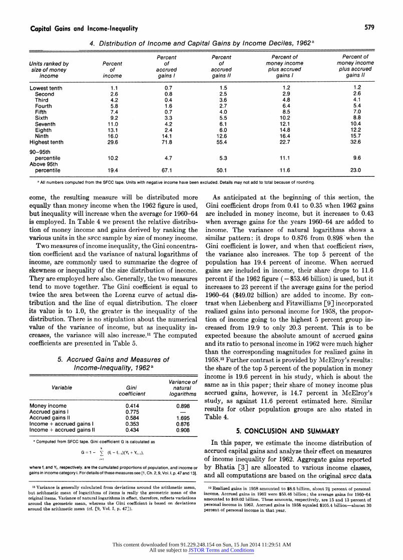
4. Distribution of Income and Capital Gains by Income Deciles, 1962a

Percent Percent Percent of Percent of Units ranked by Percent of of money income money income size of money of accrued accrued plus accrued plus accrued

income income gains I gains gains gains1

Lowest tenth 1.1 0.7 1.5 1.2 1.2 Second 2.6 0.8 2.5 2.9 2.6 Third 4.2 0.4 3.6 4.8 4.1 Fourth 5.8 1.6 2.7 6.4 5.4 Fifth 7.4 0.7 4.0 8.5 7.0 Sixth 9.2 3.3 5.5 10.2 8.8 Seventh 11.0 4.2 6.1 12.1 10.4 Eighth 13.1 2.4 6.0 14.8 12.2 Ninth 16.0 14.1 12.6 16.4 15.7

Highest tenth 29.6 71.8 55.4 22.7 32.6

90-95th percentile 10.2 4.7 5.3 11.1 9.6

Above 95th percentile 19.4 67.1 50.1 11.6 23.0

a All numbers computed from the SFCC tape. Units with negative income have been excluded. Details may not add to total because of rounding.

come, the resulting measure will be distributed more equally than money income when the 1962 figure is used, but inequality will increase when the average for 1960-64 is employed. In Table 4 we present the relative distribution of money income and gains derived by ranking the various units in the SFCC sample by size of money income.

Two measures of income inequality, the Gini concentra- tion coefficient and the variance of natural logarithms of income, are commonly used to summarize the degree of skewness or inequality of the size distribution of income. They are employed here also. Generally, the two measures tend to move together. The Gini coefficient is equal to twice the area between the Lorenz curve of actual distribution and the line of equal distribution. The closer its value is to 1.0, the greater is the inequality of the distribution. There is no stipulation about the numerical value of the variance of income, but as inequality increases, the variance will also increase." The computed coefficients are presented in Table 5.

5. Accrued Gains and Measures of Income-Inequality, 1962 a

Variance of Variable Gini natural

coefficient logarithms

Money income 0.414 0.898 Accrued gains 1 0.775 Accrued gains 11 0.584 1.695 Income + accrued gains 1 0.353 0.876 Income + accrued gains 11 0.434 0.908

a Computed from SFCC tape. Gini coefficient G is calculated as k

G =1 - E (f - ft-,)(Yi + Yi1I),

where f, and Y1, respectively, are the cumulated proportions of population, and income or gains in income category i. Fordetails of these measures see [1, Ch. 2,9, Vol. I, p. 47 and 131.

11 Variance is generally calculated from deviations around the arithmetic mean, but arithmetic mean of logarithms of items is really the geometric mean of the original items. Variance of natural logarithms in effect, therefore, reflects variations around the geometric mean, whereas the Gini coefficient is based on deviations arounid the arithmetic mean (cf. [9, Vol. I, p. 473).

As anticipated at the beginning of this section, the Gini coefficient drops from 0.41 to 0.35 when 1962 gains are included in money income, but it increases to 0.43 when average gains for the years 1960-64 are added to income. The variance of natural logarithms shows a similar pattern: it drops to 0.876 from 0.898 -when the Gini coefficient is lower, and when that coefficient rises, the variance also increases. The top 5 percent of the population has 19.4 percent of income. When accrued gains are included in income, their share drops to 11.6 percent if the 1962 figure (-$53.46 billion) is used, but it increases to 23 percent if the average gains for the period 1960-64 ($49.02 billion) are added to income. By contrast when Liebenberg and Fitzwilliams [9] incorporated realized gains into personal income for 1958, the proportion of income going to the highest 5 percent group increased from 19.9 to only 20.3 percent. This is to be expected because the absolute amount of accrued gains and its ratio to personal income in 1962 were much higher than the corresponding magnitudes for realized gains in 1958.12 Further contrast is provided by McElroy's results: the share of the top 5 percent of the population in money income is 19.6 percent in his study, which is about the same as in this paper; their share of money income plus accrued gains, however, is 14.7 percent in McElroy's study, as against 11.6 percent estimated here. Similar results for other population groups are also stated in Table 4.

5. CONCLUSION AND SUMMARY In this paper, we estimate the income distribution of

accrued capital gains and analyze their effect on measures of income inequality for 1962. Aggregate gains reported by Bhatia [3] are allocated to various income classes, and all computations are based on the original SFCc data

12 Realized gains in 1958 amounted to $8.6 billion, about 21 percent of personal income. Accrued gains in 1962 were $53.46 billion- tbe average gains for 1969-64 amounted to $49.02 billion. These amounts, respectively, are 15 and 13 percent of personal income in 1962. Accrued gains in 1958 equaled $105.4 billion-almost 30 percent of personal income in that year.




file. The results show that gains were more unequally distributed than money income in 1962. Two separate estimates of accrued gains-the accrued loss for 1962, and the average of gains for 1960-64-are used. When gains are included in income, the first measure leads to a reduction in income inequality, but the second increases it appreciably. Gini coefficient and variance of natural logarithms are selected as indicators of income inequality. No information, comparable to the SFCc data for 1962, is available for other years; therefore, a replication of all the 1962 results for other years is not possible.

5.1 A Critique By confining all our computations to the SFCC file, we

have avoided many problems of definition and approxi- mation which arise when data, especially the grouped and highly aggregative type, are combined from various sources. But this also implies that our results are subject to all the criticisms and qualifications that apply to the SFCC. The survey was unique in using very high sampling rates toward the upper end of the income scale. Many adjustments for nonresponse were also made; still, as Ferber et al. [6] discovered for corporate stock, asset holdings of higher wealth brackets might be understated. We have allocated gains according to value of assets owned by various units; consequently, our results are probably biased towards equality, but the bias cannot be measured or adjusted for.'3 Other sources of potential bias, perhaps more important than the limitations of the SFCC, might be present in the aggregate estimates of gains and in the assumptions made in linking them to the SFCC file. For example, capital gains have not been adjusted for changes in the general price level, and the gains accruing on several assets such as bonds, consumer durables, etc., have not been calculated. Considering the state of our knowledge in this area and the serious limitations of the existing data, the present study marks a solid step for- ward, although its conclusions are far from being final.

[Received June 1974. Revised June 1975.]

13 For details of adjustments for nonresponse and their effects on SFCC data (see [14, pp. 58-61; and 15, pp. 113-20]). The validation study by Ferber et al. differed from the SFCC in many respects and yielded no information on how the suspected understatements in the SFCC should be corrected (cf. [4, pp. 6, 71]).

REFERENCES [1] Aitchison, John and Brown, J.A.C., The Lognormal Distribu-

tion, Cambridge, England: Cambridge University Press, 1957. [2] Arena, John J., "Postwar Stock Market Changes and Consumer

Spending," The Review of Economics and Statistics, 47 (Novem- ber 1965), 379-91.

[3] Bhatia, Kul B., "Accrued Capital Gains, Personal Income and Saving in the United States, 1948-64," The Review of Income and Wealth, 16, No. 4 (December 1970), 363-78.

[4] , "Capital Gains, the Distribution of Income, and Taxa- tion," National Tax Journal, 27, No. 2 (June 1974), 319-34.

[5] Brimmer, Andrew F., "Inflation and Income Distribution in the United States," Review of Economics and Statistics, 53, No. 1 (February 1971), 37-48.

[6] Ferber, Robert, Forsythe, J., Guthrie, H.W., and Maynes, E. Scott, "Validation of Consumer Financial Characteristics: Common Stock," Journal of the American Statistical Associa- tion, 64 (June 1969), 415-32.

[7] Goldsmith, Selma F., "Size Distribution of Personal Income," Survey of Current Business, 38 (April 1958), 10-19.

[8] Granger, Clive W.J. and Morgenstern, Oscar, Predictability of Stock Market Prices, Lexington, Mass.: D.C. Heath and Co., 1970.

[9] Kendall, Maurice G. and Stuart, Allan, Advanced Theory of Statistics, London: Charles W. Griffin & Co., Ltd., 1963.

[10] Liebenberg, Maurice and Fitzwilliams, Jeanette M., "Size Distribution of Personal Income, 1957-60," Survey of Current Business, 41 (May 1961), 11-21.

[11] McElroy, Michael B., "Capital Gains and the Theory and Measurement of Income," IUnpublished Ph.D. dissertation, Department of Economics, Northwestern University, 1970.

[12] Miller, Herman P., Income Distribution in the United States, Washington, D.C.: U.S. Bureau of the Census, 1966.

[13] Morgan, James N., "Anatomy of Income Distribution," Review of Economics and Statistics, 44 (August 1962), 270-83.

[14] Projector, Dorothy S. and Weiss, Gertrude S., Survey of Financial Characteristics of Consumers, Washington, D.C.: Board of Governors of the Federal Reserve System, 1966.

[15] 'Weiss, Gertrude S. and Thoresen, Erling T., "Composi- tion of Income as Shown by the Survey of Financial Charac- teristics of Consumers," in Lee Soltow, ed., Six Papers on the Size Distributions of Income, New York: National Bureau of Economic Research, 1969.

[16] Schultz, T. Paul, "Secular Trends and Cyclical Behavior of Income Distribution in the United States: 1944-1965," in Lee Soltow, ed., Six Papers on the Size Distribution of Income, New York: National Bureau of Economic Research, 1969.

[17] U.S. Treasury Department, Statistics of Income, Individual Income Tax Returns, Washington, D.C.: U.S. Government Printing Office, various years.

