1
CAN POPULATION CHARACTERISTICS ACCOUNT FOR THE
VARIATION IN HEALTH IMPACTS OF AIR POLLUTION?
A Meta-Analysis of PM10-Mortality Studies.
Borghild Marie Moland Gaarder, Ph.D.University College London2002
Abstract: In this paper a regression analysis is undertaken using the largest sample of airpollution mortality studies to date, from both developing and developed countries, in anattempt to further the understanding of the relationship between suspended particles andmortality. Applying Empirical Bayes meta-analysis, it is estimated that mortality rates onaverage increase by 6 per cent per 100-µg/m3 increase in Particulate Matter (PM10)concentrations, with greater effects in countries with high income inequality. We furtherfind evidence that education and income have an influence on the effects of PM pollution.
Acknowledgements: A number of people have given me support, advice, and feedbackduring the process: my supervisors David Ulph and David Pearce at University CollegeLondon, David Maddison at CSERGE, Robert Mabro at the Oxford Institute for EnergyStudies (OIES), Torstein Bye, Knut-Einar Rosendahl, and Bente Halvorsen at StatisticsNorway, Gunnar Eskeland, Maurreen Cropper, Mead Over, Andrew Sunil Rajkumar,Kirk Hamilton, and John Dixon at the World Bank, Frank Windmeijer at the Institute forFiscal Studies (IFS), and Ulrich Bartsch throughout the process. Statistics Norway, theOIES, and the World Bank are gratefully acknowledged for having provided support andexcellent working conditions when in Oslo, Oxford, and Washington, respectively.Financial support was provided by the Norwegian Research Council.
Table of Content:I. Introduction ..................................................................................................................................................... 2II. A Survey of Existing Meta-Analyses of the Mortality from Air Pollution........................................... 3III. The Moderator Variables............................................................................................................................. 10IV. Sample Selection, Data, and Methodology.............................................................................................. 17
4.1 Sample ........................................................................................................................................................ 174.2 Data............................................................................................................................................................. 194.3 Methodology............................................................................................................................................. 25
V. Results ............................................................................................................................................................ 275.1 Main Findings........................................................................................................................................... 275.2 Sensitivity Analysis ................................................................................................................................. 335.3 Discussion................................................................................................................................................. 42
VI. Conclusion ..................................................................................................................................................... 52REFERENCES ........................................................................................................................................................... 55Appendix A: Relating the Present Study to the Maddison and Gaarder (2001) Study.................................. 72Appendix B: Mathematical Derivation of the Equations in Section 4 .............................................................. 73Appendix C: Do-file in STATA to Maximise the Likelihood Function .......................................................... 75Appendix D: Data....................................................................................................................................................... 77Appendix E: Regression Results for the Full Sample Using OLS and VWLS................................................ 83Appendix F: Regression Results for a Random Sample of Sample Combinations........................................ 85
2
I. Introduction
As early as in 1952, during the air pollution disaster in London, 1 it was established
that high levels of particulate-based smog could cause dramatic increases in daily mortality.
The relationship between particulate matter and mortality has been analysed for some time
now, and studies have reported evidence of increases in daily mortality also at much lower
levels of particle concentrations. The variability among epidemiological findings, however,
suggests that the connection between particulate matter and mortality is not well understood.
In this study we analyse the largest sample of short-term air pollution mortality
studies to date, from the widest range of countries, in an attempt to further the understanding
of the relationship between particles and mortality. In particular, our sample consists of
time-series studies examining the effect of changes in daily (averaged) air pollution levels
on daily mortality. The statistical relationship between particulate air pollution and mortality
is addressed in epidemiologic studies, and the ensuing ‘dose-response functions’ tell us the
impact on the mortality rate of a population of a certain dose of pollution. 2 Because the
epidemiologic studies differ in a number of ways, the regression coefficient of the dose-
response function is likely to vary both with the characteristics of the exposed population,
other site-specific differences, as well as analytical decisions.
This study will focus on whether population characteristics can explain some of the
differences in effect estimates, while through sample selection trying to minimise the
potential for other underlying sources for differences.
The analysis involves isolating relevant moderator variables using meta-regression
methods. A moderator variable is a variable that causes differences in the correlation
between two other variables, in this case between mortality and ambient concentration of
air pollution. If there is true variation in results across studies, then one or more
moderator variables must exist that are able to account for the variance. The general
underlying form is as follows:
∑ ++= jjkkj uZb αβ (j = 1,2…L) (k = 1,2…M) (1)
here bj is the reported dose-response estimate in the jth study from a total of L studies, β is
the summary value of b, Zjk are the variables that could explain variations amongst the
1 The London smog disaster (December 1952) established that high levels of air-borne particles and sulphurdioxide produced large increases in daily death rates (HMSO, 1954).2 For a review of the main study designs associated with epidemiologic studies refer to B. M. M. Gaarder(2002), chapter 5.

3
studies, αk are the coefficients of the M study characteristics that are controlled for, and uj is
the error term.3
The differences in results from individual studies imply that the quite commonly
used procedure of transferring the regression coefficient unchanged to another population
may lead to incorrect estimates of adverse health effects and the related costs. However,
direct studies of the population in question may often not be feasible due to the quality of
data, or to time and financial constraints. With the growing body of dose-response studies
increasingly carried out also outside of the US, a second-best option is emerging. Rather
than transferring the dose-response coefficients unaltered from one population to another,
the existing studies can be used to estimate the coefficients on relevant moderator
variables, and these in turn may enable us to transfer dose-response functions. We are
then in the position to tailor-make the coefficient for local conditions.
The meta-analysis may hence serve three main purposes: it can increase our
understanding of what affects the amount of deaths that are related to air pollution; it will
help highlight areas where further studies may be needed; and finally, through the ensuing
coefficients of the moderator variables, it may help transferring the dose-response
coefficients to countries where empirical studies have not yet been feasible or to forecast the
effects of policies targeting air pollution.
Section 2 introduces the concept of meta-analysis, as well as the various uses,
strengths, and weaknesses of this type of analysis. In section 3 we then move on to
presenting the moderator variables selected. Next, section 4 describes the criteria used in
composing our sample of past studies, the data used to capture the moderator variables, as
well as the model and estimation procedure. The main results are presented in section 5,
together with a sensitivity analysis and a discussion of the findings. Main results and
implications are summarised in chapter 6.
II. A Survey of Existing Meta-Analyses of the Mortality from Air Pollution
Meta-analysis involves the synthesising of previous empirical analyses. Before
presenting a survey of what has been done in this field, a brief introduction to the original
studies and study-designs upon which these meta-analyses are based is therefore required.
The majority of the original studies use time-series data to examine the effect of
short term responses in mortality to changes in air pollution levels. The main advantage of
time series studies over cross-sectional studies is that socio-economic and demographic
characteristics of the population are unlikely to change and do therefore not require explicit
3 Button and Nijkamp (1997).

4
modelling. The studies usually assume that the daily death counts (Yi) are Poisson-
distributed4 with:
log (E(Yi)) = Xiβ
where Xi is the vector of covariates on day i, β is the vector of regression coefficients, and E
denotes expected value. The unit of analysis in these studies is the day, and hence the
potential confounders that must be controlled for are those that vary over time, possibly in
coincidence with air pollution. Based on this logic, the vector of explanatory variables
typically contains terms corresponding to a measure of air particulate, as well as
meteorological covariates (e.g. ambient temperature and relative humidity), long-term and
seasonal trend components, disease epidemics (e.g. influenza episodes), and day of the week
and holidays.
It is important to point out that the dose-response function technique, as presented
above, is mechanistic, incorporating no model of how individuals behave. The dose-
response coefficient relies on the socio-economic and demographic characteristics
remaining unchanged. Although it can quite accurately describe the effect of a change in air
pollution on mortality in a certain population, demographically different groups and groups
subject to different economic constraints may respond differently to exposure to air
pollution. This is why, when we compare results from studies carried out at different sites,
we need to take such differences into account. That is the role of the moderator variables in
the meta-analyses.
Early meta-analyses were mainly concerned with finding the average effect across
studies, implicitly assuming that the estimated effect in each study is an estimate of an effect
size common for the whole population of studies. More recently, meta-analytic work has
started to focus upon discovering and explaining the variations in effect sizes (Raudenbush
and Bryk (1985)).
Button and Nijkamp (1997) discuss a number of issue areas within environmental
policy evaluation which could benefit from the use of the meta-analysis techniques. In
evaluating environmental costs, the meta-analysis can be used to look for indicators of
central tendency in previous case studies or, alternatively, to explain why the studies
4 Only a small portion of a population dies on any given day. The number that die is a count; i.e. it can onlytake on values limited to the non-negative integers. This suggests that a Poisson process is the underlyingmechanism modelled, since in a Poisson process a homogeneous risk to the underlying population isassumed. Given that underlying risk, the probability of Y deaths occurring on a given day is given by:
( )!y
e/yprob
Yλλ
λ−
=
where λ is the expected number of deaths on any day (i.e. E(Y)) (Schwartz et al. (1996b)).
5
generate differing results. Furthermore, meta-analysis can be used in connection with the
assessment of the effectiveness of alternative policy instruments in containing
environmental damage, the assessment of political acceptability of alternative
environmental instruments by decision makers, exploration of the appropriate political
level of intervention to contain environmental damage, and finally in forecasting the
effects of environmental policies.
Rosenthal (1991) distinguished three purposes of meta-analyses. First, to
summarise for a set of studies what the overall relationship is between two variables
investigated in each study. Second, to look at the factors associated with variations in the
nature of relationships between two variables over a range of studies. Finally, to look at
the aggregate data for each study and correlate this with other characteristics of the study
(Bergh et al. (1997)).
There is a wide range of problems involved in employing meta-analysis in
economic research. Broadly, we can divide the problems into two categories. The first
category has to do with the objectivity with which the information is collected and
reported, whereas the second deals with comparability between studies and how well the
studies are designed for the particular question they want to address. There is a possible
bias resulting from the nature of the studies that are included or excluded. First, the
researchers use various inclusion-selection rules for the analysis (e.g. including only
published studies) which are inherently subjective. Second, there is the tendency to
publish only positive results. As for comparability, a number of challenges exist. Studies
often use diverse units of output measures and, furthermore, diverse methods of obtaining
these outputs (e.g. diverse regression methods, different sets of control variables). A
degree of subjectivity is introduced into many of these studies and thereby into the meta-
analysis because the reported results were based on what, in the authors’ opinions were
the best coefficient estimates obtained. In particular, some studies reported coefficients
obtained using same day level of pollution, others used one-day lags, and others again
used moving averages of different lengths.
Estimates can differ partly due to the fact that the studies use different samples of the
total population and partly due to the differing conditions under which the research takes
place. Fixed effects models assume the existence of a common effect size in all the studies,
whereas random effects models assume a different real effect in each study. In the latter
case, combining effect sizes from empirical studies means assessing the average size of the
real effect.

6
If we reject the hypothesis of equal real effect sizes, the next question is then
whether we can find moderator variables that explain the variations between the empirically
estimated effect sizes. If a linear combination of variables exists that completely explains the
variations in the real effect sizes, then the effect size is fixed and not random (although the
real effect sizes are different in each study). This is, however, a rare case. In most cases it is
more realistic to use a model that takes account of the imperfections of the explanatory
model.
Before we review the literature of meta-analyses on studies of mortality from
particulate matter it is useful to understand the various models and assumptions underlying
the different approaches.
Let us assume that the estimated effect size di of study i is equivalent to a true effect
size δ i plus an error of estimate ei, where the errors are assumed to be independent and
normally distributed with a variance vi:
iii ed += δ , i = 1, …,k, ei ~ N(0, vi) (2)
The random effects model assumes that the effect size parameters δ i can be decomposed into
a mean population effect θ and a between-study variability term ui, where the errors are
assumed to be independent and normally distributed:
ii u+= θδ , i = 1, …,k, ui~ N(0, τ2) (3)
The mixed effects model (which is equivalent to a random effects model incorporating study
characteristics) assumes that the effect size parameter is a function of known study
characteristics and random error:
iii uW += γδ ' , i = 1, …,k, ui ~ N(0, τ2) (4)
The fixed effect model implicitly assumes no between-study variability in either of the
equations above, i.e. ui= 0.
Combining equations (3) and (1) we obtain:
iiii euWd ++= γ' (5)
Therefore, assuming that the error terms are independent, we can express the marginal
distribution of di from the mixed effect model as:
( )2' ,~ τγ +iii vWNd (6a)
The distribution of di from the random effect model, the simple fixed effect model, and the
fixed effect model with study characteristics can be expressed respectively as:
(6b) ( )2ii v,N~d τθ + , (6c) ( )ii v,N~d θ , and (6d) ( )i
'ii v,WN~d γ
7
Based on the epidemiological literature dealing with the relationship between air
pollution and mortality, to our knowledge seven meta-analyses have been carried out:
Ostro (1993), Schwartz (1994), Lipfert and Wyzga (1995), Environmental Protection
Agency (1996), Levy et al. (2000), Institute for Environmental Studies (2000), and
Maddison and Gaarder (2001).5
After converting the results of the different studies into a common metric, Ostro’s
meta-analysis derived the unweighted average of central estimates and found that the
mean effect of a 10 µg/m3 (micrograms per cubic meter) change in PM10 on the
percentage change in mortality varied between 0.64 and 1.49 per cent. Lipfert and
Wyzga, on the other hand, calculated the variance weighted average of air-pollution-
mortality elasticities and found that the mean overall elasticity as obtained from time-
series studies for mortality with respect to various air pollutants entered jointly was
approximately 0.048 (0.01 – 0.12). The elasticity obtained for population-based cross-
sectional studies was of similar magnitude. The models used in both of these meta-
analyses implicitly assume that each coefficient estimate, β , is a random sample from a
single underlying distribution with a distribution as in expression (6c). Ostro’s study in
addition implicitly assumes equal estimation errors in all of the studies.
Joel Schwartz (1994c) carried out a meta-analysis on a set consisting of studies
from the US, London, and Athens. The main aim of the analysis was to compare the
results found in different studies to the levels of potential confounders and the correlation
between particulate matter and potential confounders in the individual studies to assess
the likelihood that the results are driven by inadequate control for those factors. It then
combines the studies in a meta-analysis and computes the average percentage increase in
mortality per unit of pollution. Three approaches to calculating this average were used;
unweighted, variance weighted, and quality weighted. The latter weights were based on
the possibility in each study that the true effect sizes vary at least in part as a function of
multiple identifiable sources, or confounding variables, and that if these have not been
taken properly into account in the regression model used in a particular study the random
error term will be larger for these studies. The central concern in the study was of
confounding by some other pollutant, by weather and season, and an additional concern
was the quality of the exposure assessment. Studies were given a higher weight the more
they controlled for confounding factors (the highest weight was 4 and the lowest 2). The
unweighted meta-analysis, as well as the analyses using the various weighting options all
5 For a review of how the present study relates to the Maddison and Gaarder study, please refer to appendix A.
8
gave a relative risk of 1.06 for a 100 µg/m3 increase in total suspended particulate mass,
which implies that the relationship is highly unlikely to be due to confounding factors.6
By introducing the quality weights, Schwartz is allowing for the idea that there is no
single common underlying effect size. However, the size of the weights was provided by
the researcher based on his subjective opinion of the quality of control for confounding.
This subjective weighting may influence the results and is a weakness of the above meta-
analysis.
In its meta-analysis the U.S. Environmental Protection Agency (EPA (1996))
criteria document used a random effects model to estimate PM mortality, where the
distribution of the effect parameter is assumed to be given by expression (6b). The
relative risk for mortality from PM10 exposure averaged over 2 days or less was in this
study estimated as 1.031 per 50 µg/m3 PM10 (CI: 1.025 – 1.038), whereas for a longer
averaging time of between 3 and 5 days the relative risk was estimated as 1.064 (CI:
1.047 – 1.082). When potential confounding pollutants were included in the model the
relative risk estimate decreased (1.018, CI: 1.007 – 1.029). Although the random effects
model can quantify the amount of residual variance that can be explained by study
characteristics, it does not attempt to identify what these characteristics are or how they
influence the effect estimates.
In the most recent meta-analysis carried out by the Institute for Environmental
Studies (IVM) (2000), the purpose was to obtain a single pooled estimate of the health
effects reported from the selected studies in order to use this for evaluating the benefits
gained from improving air quality in Mexico City. A weighted average was computed,
giving more emphasis to studies with lower error in estimating their regression
coefficient, as well as studies carried out in Mexico city (‘articles with estimates based on
Mexico City were given double the weight of international cases, because they are more
likely to reflect the socio-demographic and susceptibility characteristics of the Mexico
City population’ (p.27, IVM (2000)). The pooled estimate of the effect of PM10 on total
mortality was 0.79 per cent change per 10 µg/m3 daily average PM10 (CI: 0.06 – 1.68).
There is a certain inconsistency/contradiction in the method they have used. By
weighting the estimates according to the inverse of their variance, the study is assuming
that the variability in reported effects is attributable solely to sampling error. On the other
hand, giving higher weights to the studies carried out in Mexico City implies that the
6 The information concerning the effect from exposure to air pollution on the risk of mortality uncovered byregression analysis can be expressed in a number of alternative ways. The findings are often expressed in termsof relative risk. The relative risk indicates the ratio of the probability of occurrence of a given effect between

9
authors assume that these studies are capturing some local characteristics and are hence
more relevant for the purpose of policy-evaluation in Mexico City. This is a rather
indirect way of controlling for confounding factors and may weaken the reliability of the
pooled estimates. Furthermore, as was the objection to Schwartz’ study, the size of the
weights was provided by the researcher on a rather ad hoc basis and may influence the
results.
Rather than providing pooled effect estimates, the meta-analysis by Levy et al.
(2000) addresses between-study variability potentially associated with analytical models,
pollution patterns, and exposed populations. They use the mixed effects Empirical Bayes
(EB) model derived by Raudenbush and Bryk (1985), assuming that variability is due
partly to sampling errors (or intra-study variability) and partly to between-study
variability. This method is used in the present study as well, and the details of the method
are set out in section 4.3. With a sample of 29 observations, 19 from the United States
and 10 from outside of the United States, they investigate whether the ratio of PM2.5 to
PM10, other pollutants, climate, season, prevalence of gas stoves and/or central air
conditioning, percentage of elderly, percentage in poverty, and the rate of mortality can
explain some of the differences in effect estimates. When analysing the 19 PM studies
from the U.S. for which more confounding variables were available, the mortality rate
was estimated to increase by 0.7 per cent per 10 µg/m3 increase in PM10 concentrations,
with greater effects at sites with higher PM2.5/PM10 ratios, supporting the hypothesised
role of fine particles. When all of the 29 studies were included, but only a subset of the
predictors were available (PM10 concentration, averaging time and lag time, percentage
of the population older than 65 years of age, baseline mortality rate, heating and cooling
degree days, and dummy variables for PM10/TSP and U.S./non-U.S. studies) only
baseline mortality rate was significant. The grand mean estimate was about the same as
for the 19-studies sample.
Finally, the meta-analysis by Maddison and Gaarder (2001) investigates whether,
in a sample of 13 European and developing country studies, some of the between-study
variability can be associated with pollution levels, the percentage of the population over
65 years of age, average income level, and the level of income inequality at a certain
average income level. By weighting the effect estimates according to their estimated
variances, we implicitly assumed a fixed effect model with study characteristics for which
the distribution was given in expression (6d). The study found that the effect estimates were
two different exposure levels or exposure groups.
10
significantly affected by the percentage of the population over 65 years of age, as well as
income distribution. Based on the data used in our study, a model without predictors (i.e.
fixed effect model) gives an estimate of the effect of PM10 on total mortality of 0.3 per
cent change per 10 µg/m3. An implicit assumption of our analysis, which seems unlikely
and therefore weakens the results of this study, is that all the variance among the study
effects other than sampling variance can be explained as a function of the study
characteristics we chose to include.
In addition to the meta-analyses discussed above, a number of review articles
have relied on qualitative discussions of the credibility of the evidence related to potential
confounding factors (e.g. climate, correlated pollutants). Some of the authors of these
studies conclude that a causal relationship clearly exists (Brunekreef et al. (1995), Pope et
al. (1995a), Pope et al. (1995b), Thurston (1996)), whereas others (Gamble and Lewis
(1996), Moolgavkar and Luebeck (1996)) argue that the relationship is spurious. The lack
of quantitative base, however, makes these review studies more vulnerable to the set of
studies chosen and the points the authors wish to argue. (Levy et al. (2000)).
III. The Moderator Variables
As mentioned in section 2, the original studies do not explicitly model the
demographic and socio-economic characteristics of the population studied. The reason
for this is that for a factor to confound the relationship between pollution and daily
mortality it must be correlated with both pollution and mortality. Therefore,
characteristics such as baseline health, age, and income cannot induce an association
between today’s mortality count and yesterday’s air pollution, since they are not
correlated with air pollution and do not vary on a daily basis.7 For cross-sectional
mortality studies, on the other hand, personal characteristics and habits are important
potential confounders, whereas short-term weather changes are not (Schwartz (1994c)).
In our meta-analysis the aim is to combine time-series studies cross-sectionally, and to
explain the variation in the dose-response coefficients using moderator variables (also
known as effect modifiers). These moderators will hence need to address cross-sectional
differences, rather than factors changing over time.
When deciding on which study-characteristics to include as potential predictors or
moderator variables three factors guided the selection; theoretical plausibility, availability
of characteristic-data, and novelty. This led to the following moderator variables; mean
7 The most important confounders for the relationship between air pollution and daily mortality are weatherand infectious disease epidemics, according to Schwartz (1994c).
11
particle levels, amount of elderly people in the population, income level, income
distribution, education, baseline health, and health services.8 The reasons why we believe
these factors (or characteristics) to be potential moderators are discussed below. Other
study characteristics, such as the lag and averaging times, the levels of other pollutants,
the ratio of fine particles to overall particle concentration, and the type of mortality
considered, although potentially interesting predictors, were either not considered due to
lack of information in many of the studies or were investigated through sensitivity
analysis.
Most dose-response analyses have implicitly assumed a log-linear relationship
between the mortality count and pollution, however, it has been argued that this may not be
accurate. As the exact shape of the relationship is not yet known, we argue that it may be
interesting to include pollution as a moderator variable. By regressing the estimated
pollution-mortality association on pollution (i.e. second order partial derivative), we pick up
any non-linearities in the relationship.
A variety of advanced disease states, as well as generally lower baseline health
levels, may predispose individuals to heightened susceptibility to premature death due to
exposure to air pollution. This implies that the death rate due to a certain amount of
particle exposure may increase more among elderly and individuals with lower baseline
health as compared to the younger and those with better health, and that death rates due
to respiratory and cardiovascular failure increase more than the total rate. However, as
exposure tends to be approximated by air pollution concentration measurements from
central monitoring stations, it is possible that the individual exposure for a certain amount
of pollution concentration also varies with baseline health levels and age (i.e. the optimal
amount of averting activities may be affected by age and health level). Furthermore, the
heightened susceptibility to exposure may influence the amount of mitigating activities
chosen by elderly individuals and individuals with low levels of baseline health. In other
words, both age and baseline health levels may well influence the amount of mitigating
and averting activities undertaken, and hence affect health indirectly. On the one hand, it
is possible that an individual with low health levels will be more inclined towards trying
to prevent further adverse health effects (both due to personal experience with bad health
and due to decreasing utility at an increasing rate). On the other hand, the individual may
be used to being in bad health and expect to live for a shorter time, and therefore less
inclined to invest in health. It is theoretically not clear what net effect baseline health and
8 The first four were also used in the Maddison and Gaarder meta-analysis.

12
age will have on the concentration-response coefficient, but both characteristics may
certainly play a role and should therefore be included as moderator variables.
Empirical dose-response studies have found that mortality among the elderly is
more responsive to changes in particulate pollution than is mortality for the entire
population or mortality among the younger generation (Ostro et al. (1996), Schwartz and
Dockery (1992a)). Evidence further suggests that air pollution has its greatest adverse
effects on people with pre-existing chronic conditions such as asthma, bronchitis, and
emphysema (Ostro (1987)).
Age and baseline health will tend to be closely associated when looking at entire
populations. In particular, if a population has a large percentage of elderly people it
indicates that the baseline health of that population is rather high, enabling so many to
live to an old age. Hence, if the baseline health variable is omitted from the regression
analysis the age-variable, which is supposed to pick up the part of the population that is
most at risk from high air pollution, will also proxy for the average health level of the
population. These are two offsetting effects, and age will hence tend to be biased
downwards. Baseline health levels will tend to be associated with level of income,
although the association will probably be highly sensitive to the measure used for
baseline health. Low-income individuals may have worse baseline health levels if low
income and little education have given rise to wrong and/or insufficient nutrition and
other health investments in the past.9 On the other hand, people who have a history of
chronic obstructive pulmonary disease or cardio-pulmonary problems are also thought to
be particularly vulnerable, and these types of health problems are more pronounced in
high-income groups and countries.
There are several reasons why one would expect the increase in mortality due to
ambient particles to vary with income.10 Firstly, for a certain increase in ambient
concentration of air pollution we argued that lower income groups were likely to
experience a larger increase in exposure than were the higher income groups because the
former are not being able to afford much averting activities (e.g. sealing houses to reduce
the penetration of outdoor pollutants, using less-polluting heating and cooking fuels,
spending less time in traffic). Secondly, for a certain amount of exposure and its
anticipated health effect we suggested that the behavioural response (e.g. visiting a
doctor, taking medication) will typically be influenced by income level. These mitigating
measures imply costs which poor people may not be able to afford, or willing to pay
9 Refer to B.M.M. Gaarder (2002), section 5.4.3 in chapter 5.10 Refer to chapter 5 in B.M.M. Gaarder (2002) for a more detailed discussion.
13
given their budget constraints. Finally, we argued that there may be differences between
low and high income groups, and even more so between low and high-income countries,
in the extent to which official mortality statistics reflect actual mortality. It is not unlikely
that deaths among the poor will be underrepresented or unavailable in official statistics.
Although this latter point may imply an under-representation of the increase in mortality
due to air pollution in lower income groups or countries, we suggest that the overall
measured adverse health effects of an increase in air pollution will tend to be larger in
low-income countries than in higher-income countries. Income should therefore be
included as a mediator variable.
There are additional reasons why exposure may differ between developed and
developing countries, and why an increase in exposure may lead to a larger increase in
mortality in low than high-income countries that are not necessarily due to income levels,
although income may be part of the underlying explanation for these factors. Firstly, the
effect of an increase in pollution on exposure may be larger in low than high-income
countries due to the fact that many low-income countries are situated in warm climates
and the residents in these climates are therefore likely to spend a greater portion of their
time outdoors (Ostro (1994)). Other differences between low and high-income countries
may also influence the amount of time spent outdoors, such as crime rates, indoor air
pollution, and social interaction traditions. Furthermore, the pollution level locally at the
work place may be higher in less developed countries due both to the cost of abatement
and less strict work place regulation. Finally, an increase in exposure may lead to a larger
increase in mortality in low than high-income countries due to the quality and availability
of health care. In addition to the often very restricted availability of health care, the
quality of health care in developing countries is often poor, something which may affect
the efficiency of mitigating measures. Hence, the risk of dying from the health effect of
air pollution may be influenced by own behaviour or by the facilities available, and could
be higher for lower income groups or cities. Due to the lack of reliable data on
availability and quality of health care, time spent outdoors, work place pollution etc.,
such variables have in general not been included as moderator variables. By excluding
these from our analysis, we implicitly allow income to proxy for their effects.
There are at least three reasons to believe that the income distribution in a
country, i.e. relative income, is important for the difference in health effects. First, unless
the effect of income on the dose-response coefficient is linear, using an average income
variable will not capture correctly the sum of the effects of each individual’s income on
his or her adverse health. In particular, there are probably decreasing returns to averting

14
and mitigating activities which would imply a tendency for higher inequality to be
associated with higher mortality rates.11 Second, the location at which people live within
a city will affect the amount of air pollution they are exposed to. Although individuals
can move between cities, it seems likely that for most cities housing prices are
determined by within-city demand. Hence, it is not so much the income level as the
position within the income distribution that determines where an individual lives. If
individuals with relatively low income tend to live in the most polluted areas, as evidence
suggests, and if the adverse effect of air pollution is larger on lower income individuals
(due to lower baseline health, less education etc.), then this would once again imply a
larger PM10-mortality in cities with large income-inequality. 12 Third, there is a line of
research that implicates the biochemical effects of psychological stress as a risk factor,
and relates this stress to social status (Deaton and Paxson (1999)). Social status can then
be modelled as income relative to the average income. If mortality is associated with
stress, and stress is related to social status (income relative to the average income), then
this is a third reason why higher income inequality may lead to a larger mortality rate
from air pollution. GINI may be proxying for inequalities in baseline health or for the
quality and availability of health care, if satisfactory measures for these two variables are
not available.
It may also be of interest to consider whether the effect of income inequality on
the mortality rate from air pollution varies according to the average level of income at
which the inequality takes place. On the one hand, one could speculate that high income
inequality in a low-income country would imply a large amount of people not being able
to undertake any averting and mitigating activities whatsoever (demand-side), and that
only a small increase in income and health investment for these population groups
therefore would have a large effect in reducing mortality. On the other hand, the range of
averting and mitigating measures available to the public (the supply-side) and the
information about the effects of pollution and how to minimise these may well be larger
in high-income countries, implying that the way in which income is distributed may play
a more significant role in determining the amount of deaths caused by particulates.
Furthermore, high income-inequality in high-income countries may arguably lead to
11 There are several reasons why we find decreasing returns to health investment likely. First, it isreasonable to assume that the most cost-efficient measures are undertaken first. Second, it is not unlikelythat a similar health investment measure has a larger positive effect at high levels of exposure and lowlevels of baseline health than at lower levels of exposure and better health levels, and the two lattercharacteristics tend arguably to be associated with higher income groups.12 A cautionary remark is in order: if the effect of air particles on mortality were to be increasing at adecreasing rate, then the above finding would not necessarily hold. Empirical evidence so far, however,
15
more psychological stress than in low-income countries. For the above reasons, we
suggest considering both the effect of a relative income-inequality measure, as well as an
income distribution measure that takes the average level of income into account as
moderator variables in the regression analysis.
The income variable we ideally would like to have is the average income in the
location in question (be it a city or otherwise), or even more precisely, the average
income of the vulnerable population within the relevant location. We were not able to
obtain this information, however, and had to settle for a second-best option, namely the
average income in the country in question. If the average level of income is similar in the
study location as it is in the country as a whole, this will be a satisfactory approach.
However, it is not unlikely that for the study locations, most of which are relatively large
cities, this will not be the case. If the average income level in large cities differs in a
consistent manner from the country average, then it is possible that the best way of
capturing the average city-income is a composite of the average country income and the
income distribution in the country.
The level of education may affect the knowledge people have about health, health
production, and the connection between air pollution and health, and hence affect the
level of baseline health, as well as the amount of averting and mitigating expenditures
undertaken and the efficiency of these expenditures. Although there is conflicting
evidence as to whether little knowledge/education leads to over or under-investment in
health, we suggest that education should be included as a moderator variable. Since
schooling is closely associated with income, the income coefficient will probably proxy
for this variable if it is not included as a moderator variable.
Finally, the health services provided in a country are likely to influence the
amount and severity of adverse health incidences. Health services are likely to be highly
positively correlated with baseline health and the amount of people over the age of 65,
and negatively with income inequality.
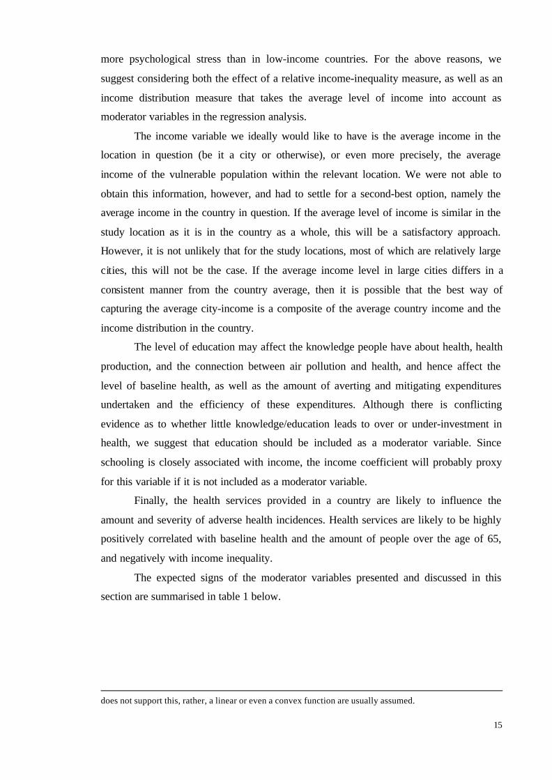
The expected signs of the moderator variables presented and discussed in this
section are summarised in table 1 below.
does not support this, rather, a linear or even a convex function are usually assumed.
16
Table 1: Summary of the expected signs of the moderator variables in a table
Expected Signs of Moderator VariablesModerator variable SignAir Pollution +Baseline Health -Age +Income -Income Inequality +Composite Variable (Interaction Variable)of Income and Income Distribution ?Education -Health Services -
All of the above mentioned variables are potentially important moderator variables,
especially when transferring estimates to cities in developing countries which may take
substantially different values on all of these. The level of air pollution is in general
significantly higher in many developing countries than in the developed countries that
generated most of the literature. Furthermore, an important difference between developed
and developing countries is that the former tend to have an ageing population, whereas
the latter have a majority of young people (higher birth-rate and lower life-expectancy),
and we therefore find it potentially interesting to include this moderator variable. A
crucial difference between developed and developing countries is the lower average
income level in the latter. In addition, income in developing countries tends to be more
unequally distributed (the average GINI-coefficient for the low-income countries in the
World Development Report 1998/99 is 0.41, and for the high-income countries it is 0.30).
As for health levels and education, these are both closely associated with income and thus
typically on average much lower in developing countries than in their richer counterparts.
If the original studies have not satisfactorily controlled for confounding variables
such as other pollutants, the ratio of fine particles to overall particle concentration,
temperature, season, and humidity, and if these are correlated with the measured ambient
particles, the resulting dose-response coefficients may be biased. However, assuming that
the original studies have (linearly) controlled for various confounding factors, these may
still have an impact on the measured effect size of air pollution on mortality. As
information on these variables was missing in many of the studies in our sample such
moderator variables were left out. However, a meta-analysis focussing on such
confounding variables was carried out by Levy et al. (2000).

17
IV. Sample Selection, Data, and Methodology
4.1 Sample
The sample on which we perform the meta-analysis is composed of time-series
studies gathered from previously published meta-analyses or review articles (Maddison
and Gaarder (2001), Levy et al. (2000), Institute for Environmental Studies (2000)), as
well as from PubMed.13
The selection of the wider sample is based on the following criteria for inclusion:
1. papers including the quantification of either Total Suspended Particles (TSP), Black
Smoke (BS), or Particulate Matter (PM) larger than 2.5 µm in diameter;
2. published papers evaluating the association between exposure to particles and total
mortality;
3. mortality figures modelled using Poisson regression analysis;
4. studies carried out on a representative sample of the population (e.g. excluding
studies carried out on particular age groups); and
5. analysis controlling the confounding effect due to meteorology and temporal effects.
Papers not presenting information on the variance, standard error, or confidence
intervals of the estimated coefficient were excluded. Furthermore, papers reanalysing the
same site and time period (either by the same or different authors) were excluded on the
grounds of double counting. Instead of restricting the sample to APHEA and any
available developing country studies, as we did in the Maddison and Gaarder study
(2001),14 all available studies were included. In total, 70 estimates from 56 studies and 21
countries were selected.
A number of factors potentially influencing the estimated dose-response
coefficients were not used as criteria for inclusion or exclusion, but were rather the
subjects of sensitivity analyses. In the case of the total mortality measure, we found it
interesting to investigate whether inclusion of studies looking at all-cause mortality rather
than just non-accidental mortality had a significant effect on the regression results.
Similarly, testing the sensitivity of our findings to the air particle measurements used, as
well as the lag structure, could potentially yield new insights into the underlying relationship
between air pollution and mortality.
13 PubMed, a service of the National Library of Medicine, provides access to over 11 million citations fromMEDLINE and additional life science journals.14 This was mainly based on 7 time-series studies (10 observations) resulting from the APHEA project forEuropean cities (see Katsouyanni (1997) for an overview). The sample was supplemented with studies fromChile (Ostro et al. (1996)), Sao Paolo (Saldiva et al. (1995) and Delhi (Cropper et al. (1997)).
18
A further factor likely to affect the estimated association between exposure and
health in low and high-income countries differently is the way in which exposure has
been measured. As adequate information on indoor air pollution in different countries
was not available this factor could not be subjected to a sensitivity analysis, however, it
will be important to keep in mind when interpreting our results. Ambient pollution at
central monitoring stations may be particularly ill-suited to capture particulates exposure
in low-income countries. Studies have found that indoor air pollution levels are as high if
not higher than outdoor levels in several developing countries due to lack of air
conditioning and some indoor sources present (e.g. Chestnut et al. (1998), Baek et al.
(1997)). If it is vulnerable people (low baseline health levels, or of higher age) who tend
to die from air pollution, and if indoor air pollution does not strongly covary with outdoor
air pollution from day to day, then the exposure-response association may be much larger
but not be captured by studies that use readings from central monitoring stations to
measure exposure. In other words, those who are vulnerable to outdoor air pollution may
already have died from indoor air pollution. 15
As for the amount of pollutants included in the regression model, it could be used
neither as inclusion/exclusion criteria, nor as a subject for sensitivity analysis. The main
reason for this is that many studies were unclear as to whether the final results they reported
for the particulate mortality coefficient were actually based on single, dual, or multiple
pollution models. From the studies that did express clearly the amount of pollutants involved
in their regressions we know, however, that a large majority of the time-series studies
included in our sample feature single-pollutant rather than multi-pollutant regressions. The
potential drawbacks of both single and multiple pollutant regressions are discussed briefly
below.
Some epidemiologists are uneasy with the reliance on single pollutant regressions
because different pollutants tend to be highly correlated (Moolgavkar et al. (1995)). They
argue that it is premature to single out one of them as being responsible for the observed
correlation between air pollution and mortality. Furthermore, the use of single pollutant
models renders the interpretation of the available evidence difficult, since it is not known
if the deaths attributed to the different air pollutants are additive or not. Finally, choosing
15 Studies (e.g. Baek et al. (1997), Chestnut et al. (1998), Janssen et al. (1998)) comparing indoor andoutdoor concentrations of air pollution found the difference to be attribuable in part to human indooractivities (e.g. type of stove used for cooking and heating, ventilation, tobacco smoke). Clearly, the moreindoor air pollution is attributable to indoor activities, the less indoor air pollution will covary with outdoorair pollution.
19
one pollutant as a marker for air pollution can lead to under-estimation of the problem if
in fact several air pollutants are responsible.
The use of single pollutant regressions has been defended in the literature by
Schwarz et al. (1996b). They argue that given the correlation between the pollutant variables
and the relatively low explanatory power of air pollution for mortality, including multiple
pollutants in the regression risks letting the noise in the data choose the pollutant.
We will assume that the studies selected on the basis of our selection criteria were
independent samples from a random distribution of the conceivable population of studies. In
section 4 we will return to this issue and discuss why this assumption may be difficult to
support.
4.2 Data
A number of airborne particulate measurement methods have been used in exposure-
response studies. Gravimetric (weight) measurements of collected particles yield direct
measurements of airborne particle mass. The high-volume sampler collects and measures the
mass of total suspended particulates (TSP), whereas more recent samplers include devices to
selectively collect and measure the mass of various size fractions of PM (e.g. PM10, PM13,
PM2.5). Two optical, and thus indirect, methods of measuring the mass of collected particles
have also been frequently used. The black smoke (BS) method is based on light reflectance
from particle stains on sample collection filters, whereas the coefficient of haze (COH)
method is based on light transmission through the filter stain. According to the EPA,
credible estimates of particle concentrations (in µg/m3) can only be made via site-specific
calibration against mass measurements from collocated gravimetric sampling devices. (EPA
(1996), Vol. I, 1-6). The correlation between the different particle measures may have
seasonal, meteorological, and geographical variations, and the fact that various particle mass
measures are employed in different studies therefore complicates using any particular
particle measure as indicator of airborne particulates. Some measurement error is necessarily
induced by using common converters.
Each study in the meta-analysis supplied mean values of daily data over the study
period (often from several monitoring sites) for either TSP, BS, or PM. TSP and PM13 were
converted to PM10 using the factors of 0.55 and 0.77, respectively, and black smoke was
considered equal to PM10. Note that this implied dividing the estimated coefficients in
studies using the TSP and PM13 measures by 0.55 and 0.77, respectively, in order to convert
these into being PM10 or BS effects. When converting TSP to PM10 we relied on the estimate
20
of EPA,16 which suggested that PM10 is between 0.5 and 0.6. of TSP. We chose the mean of
0.55 as our conversion factor. As for BS, data from co-located BS and TSP monitors17
suggest an average ratio of BS/TSP of 0.55, and it is therefore assumed BS is roughly
equivalent to PM10. The conversion factor for PM13 to PM10 was simply obtained by
dividing 10 by 13. A few studies used both BS and TSP as particle measures, and in these
cases we chose the TSP measure, a gravimetric measure and therefore more straightforward
to convert to PM10. Particles in ambient air are usually divided into two groups according
to size: fine (diameter less than 2.5 µm) and coarse (diameter larger than 2.5 µm). The
two size fractions tend to have different origins, composition, and health effects and this
makes conversions from fine particle measures to coarse problematic. PM2.5 and COH
are essentially fine particle measures, and studies using these measures have been
excluded from the present analysis.
The proportion of population over 65 (OVER65) was used as a measure of the
segment of the population that empirically has been found to be most at risk from the
acute effects of air pollution. These data were obtained on a country-level from the World
Bank (SIMA).18 The SIMA data-base provided yearly observations on the percentage of
the population over 65 years of age for all the study countries and all the required years.
The OVER65-measure used in our regression analysis is hence the average for the
relevant study period. Studies carried out in the same country may therefore have
different OVER65-measures because they were carried out in different time periods.
Three cautionary remarks are in order. First the studies are carried out in specific
geographical ent ities within a country that do not necessarily have the same age
distribution in their population as the country overall and this may therefore introduce
some degree of measurement error into our regression analysis. Second, the impacts of air
pollution on deaths by age group may be very different in low-income than in high-
income countries. Cropper et al (1997) found that in Delhi peak effects occurred in the 15
to 44 age group, whereas in the US peak effects occur among people 65 and older.
Finally, certain studies have also found that young children may be more susceptible than
the average population to high levels of air pollution. A large proportion of people over
65 will tend to be negatively correlated with the proportion of young children, and this
may thus bias the OVER65 variable downwards.
GNP per capita at purchasing power parity (PPP) is used as a measure of average
16 See EPA (1982).17 See Cummings and Waller (1967).
21
income in the regression analysis. PPP GNP is gross national product converted to
international dollars using purchasing power parity rates.19 An international dollar has the
same purchasing power over GNP as a U.S. dollar has in the United States (i.e. the same
amounts of goods and services can be purchased in the domestic market as a U.S. dollar can
in the United States). Estimates on PPP GNP were obtained from the World Bank (SIMA).
The SIMA data-base provided yearly observations for most of the study countries from
1975 onwards. The income measure used in our regression analysis is hence an average
for the relevant study period. Main weakness of the measure is the fact that the income
level in the location where the study was carried out may differ significantly from the
overall income level of the country.
The GINI-coefficient was used to measure inequality in the income distribution of a
country. The Gini-coefficient measures the extent to which the distribution of income
among individuals or households within an economy deviates from an equal distribution. A
Lorenz curve plots the cumulative percentages of total income received against the
cumulative number of recipients, starting with the poorest household. The Gini-coefficient
measures the area between the Lorenz curve and the line of absolute equality, expressed as a
percentage of the maximum area under the line. Hence, a Gini-coefficient of zero represents
perfect equality, and an index of 100 implies perfect inequality (World Development
Indicators 2000). Estimates of the Gini-coefficients were obtained from the World Bank
(SIMA). It is important to note, however, that the number of observations over time is
very limited for most countries, and furthermore that national data differ greatly in terms
of how data are collected and expressed (e.g are the coefficients calculated for income or
consumption, gross income or taxable income, household income or individual income?).
Furthermore, the income distribution of the cities in the meta-studies are not necessarily
the same as the overall income distribution of their respective countries. The GINI-
coefficients will therefore most probably measure income distribution with some degree
of error.
The interaction term between the GINI-coefficient and GNP per capita, DIST, will
reveal whether the effect of the distribution of income on the slope of the dose-response
function differs between low- and high-income countries.
18 SIMA is the World Bank's internal database system containing more than 40 databases from the Bankand other international institutions.19 Purchasing power parity conversion factor is the number of units of a country’s currency required to buy thesame amounts of goods and services in the domestic market as U.S. dollar would buy in the United States.Purchasing power parity conversion factors are estimates by World Bank staff based on data collected bythe International Comparison Programme (World Development Indicators 2000).

22
Several measures of education were considered; enrolment ratios (education
participation), expected years of schooling and illiteracy rates (education outcomes), as
well as indicators for education efficiency. Out of these indicators only data on net and
gross enrolment ratios were available for a large number of countries (and all of the
countries included in the analysis). The gross enrolment ratio is the ratio of total
enrolment, regardless of age, to the population of the age group corresponding to the
relevant level of education, whereas the net enrolment ratio is the ratio of the number of
children of official school age actually enrolled in school to the population of the
corresponding official school age. Because the gross enrolment ratio necessarily also
includes repeaters, a high ratio does not necessarily indicate a successful education
system. For this reason we have chosen net enrolment as the preferred
education/knowledge indicator. A drawback of the latter indicator is that children who
start school at an age earlier or later than the official school age will not be included in
this ratio. More generally, enrolment does not reflect actual attendance, and there may be
reasons for overstating enrolments if for example teacher pay is related to student
enrolment. Two net enrolment ratios were available; one for primary and one for
secondary education. Net enrolment in secondary education was chosen as our education
indicator (EDUC) because the majority of the countries in our sample had a net primary
enrolment ratio of 100 percent, rendering the latter indicator powerless as a moderator
variable. Observations on net secondary enrolment ratios were available for all the
countries in the analysis back to 1980. The data for net secondary enrolment ratio was
once again obtained from SIMA, and were available from 1980 onwards. They were
averaged over the relevant study period. A measurement error may have been introduced
due to the fact that enrolment ratios locally may differ from country-level ratios.
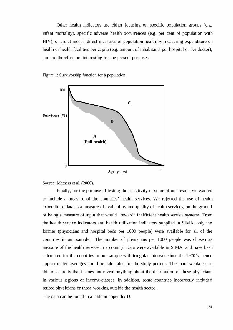
Two principal approaches are used to provide summary measures of population
health. Disability-Adjusted Life Expectancy (DALE) summarises the expected number of
years to be lived in the equivalent of ‘full health', i.e. adjusted to take account of time
lived with a disability or illness. Disability-Adjusted Life Years (DALYs), on the other
hand, are a gap measure; they measure the gap between a population’s actual health and
some defined goal (a long life free of illness and disability). The relationship between
life-expectancy at birth (LEAB), DALE, and DALYs can easily be shown with the help
of a graph depicting survival curves (figure 1). The survivorship curve (bold line in figure
1) indicates, for each age along the x-axis, the proportion of an initial birth cohort that
will remain alive at that age. Life expectancy at birth is equal to the total area under the
survivorship curve (i.e. it equals areas A+B). Area A is time lived in full health, whereas
23
area B is time lived in a health state that is less than full. Disability-adjusted life
expectancy weighs the time spent in B by the severity of the health states that B
represents before adding it to the area below the full-health-survivorship curve (i.e. area
A). Finally, disability adjusted life years quantify the difference between the actual health
of a population and some stated goal for population health (in figure 1 the health goal is
to live in ideal health until the death-day). DALYs weigh the time spent in B by the
severity of the health states that B represents before adding it to the area above the full-
health-survivorship curve, i.e. area C. (Mathers et al. (2000)).
DALE is estimated using information on the fraction of the population surviving
to each age (calculated from birth and death rates), the prevalence of each type of
disability at each age, and the weight assigned to each type of disability. Survival at each
age is adjusted downward by the sum of all the disability effects, each of which is the
product of a weight and the complement of a prevalence (the share of the population not
suffering that disability). The adjusted survival shares are then divided by the initial
population to give the average number of equivalent healthy life years that a new-born
can expect. If we enumerate health states, S, using a discrete index h, DALE can be
calculated as follows:
∑∫ ×=h
L
xhhx du)u(S)u(wDALE
where wh is weight, u represents age, and the integral is over ages from x onwards (L
represents the end of the life-time).
The DALE estimate for the population of each country was found in the World
Health Report, Annex Table 5, of the World Health Organisation. As this is a relatively
newly developed health indicator, estimates were available for 1999 only. Although this
is an indicator that may not be changing rapidly, it will nevertheless be an unprecise
measure of baseline health, especially in the older studies.
Although an individual with low health levels is more likely on average to die
relatively early compared to an individual with higher health levels, life-expectancy at
birth (LEAB) is an inaccurate measure of population health since it does not take illness
and disability into account. The advantage of this measure is that it was available in
SIMA, and has been calculated for the countries in our sample with irregular intervals
since the 1970’s. LEAB therefore offers the possibility, although imperfect, of adjusting
our health measure to reflect the period in which a particular study was carried out.
24
Other health indicators are either focusing on specific population groups (e.g.
infant mortality), specific adverse health occurrences (e.g. per cent of population with
HIV), or are at most indirect measures of population health by measuring expenditure on
health or health facilities per capita (e.g. amount of inhabitants per hospital or per doctor),
and are therefore not interesting for the present purposes.
Figure 1: Survivorship function for a population
Source: Mathers et al. (2000).
Finally, for the purpose of testing the sensitivity of some of our results we wanted
to include a measure of the countries’ health services. We rejected the use of health
expenditure data as a measure of availability and quality of health services, on the ground
of being a measure of input that would “reward” inefficient health service systems. From
the health service indicators and health utilisation indicators supplied in SIMA, only the
former (physicians and hospital beds per 1000 people) were available for all of the
countries in our sample. The number of physicians per 1000 people was chosen as
measure of the health service in a country. Data were available in SIMA, and have been
calculated for the countries in our sample with irregular intervals since the 1970’s, hence
approximated averages could be calculated for the study periods. The main weakness of
this measure is that it does not reveal anything about the distribution of these physicians
in various regions or income-classes. In addition, some countries incorrectly included
retired phys icians or those working outside the health sector.
The data can be found in a table in appendix D.
L0
100
Survivors (%)
C
A(Full health)
BB
Age (years)
25
4.3 Methodology
In this section we will briefly compare two alternative regression methods, derive
the log likelihood function for the mixed effect Empirical Bayes model, as well as
describe the tests for homogeneity and for outliers.
In order to obtain the coefficients of the moderator variables two alternative
regression methods will be described and briefly compared. In Variance-Weighted Least
Squares regressions (VWLS), the concentration-response functions are weighted
according to the statistical precision of the studies using the inverse of the variance of
each study. This is the method used by Maddison and Gaarder (2001). VWLS differs
from Ordinary Least Square (OLS) in that homogeneity of variance is not assumed – the
conditional variance of the dependent variable is estimated prior to the regression. VWLS
treats the estimated variance as if it were the true variance when it computes standard
errors. This method implicitly assumes that all the variance among the study effects other
than sampling variance can be explained as a function of known study characteristics (i.e.
there is no unexplained between-study variability). We consider this an unrealistic
assumption, and note that when available knowledge is insufficient to account for the
between-study variation, the model is misspecified. The Empirical Bayes method offers a
way of dealing with the insufficiency of knowledge, in particular; it allows us to model
the variation among the effect sizes as a function of study characteristics plus error.
Empirical Bayes is therefore the main method used in this paper.
According to Raudenbush and Bryk (1985), the Empirical Bayes meta-analysis
can be considered a special case of a two-stage hierarchical linear model. The first stage
consists of estimating a within-study model separately for each study, and at the second
stage a between-study model explains variation in the within-unit parameters as a
function of differences between units. This distribution of the true effect size consists of a
vector of known constants representing differences between the studies, a vector of
between-study parameters, and a random error term, and it is referred to as the prior
distribution of the true effect size. Empirical Bayes methods provide a general strategy for
estimation when many parameters must be estimated and the parameters themselves
constitute realisations from a prior probability distribution.
Estimates can differ partly due to the fact that the studies use different samples of the
total population and partly due to the differing conditions under which the research takes
place. Fixed effects models assume the existence of a common effect size in all the studies,
whereas random effects models assume a different real effect in each study. In the latter
26
case, combining effect sizes from empirical studies means assessing the average size of the
real effect. The common or average effect can be found by calculating the variance weighted
average of the effect sizes found, and will be called βw. In order to choose whether the fixed
or the random effects model is the most appropriate, we can perform a homogeneity test
using Cochran’s Q-statistic defined as:
( )∑
=
−=
k
i i
wi
vQ
1
ββ (9)
where vi is the variance of the reported effect from study i, βi. If the sample size is large in
each study, Q asymptotically has a X2-distribution with k-1 degrees of freedom. The
hypothesis of homogeneity will be rejected if the value of Q is large.
If we reject the hypothesis of equal real effect sizes, the next question is then
whether we can find moderator variables that explain the variations between the empirically
estimated effect sizes. If a linear combination of variables fully explains the variations in the
real effect sizes, then the effect size is fixed and not random (although the real effect sizes
are different in each study). This is, however, a rare case. In most cases it is more realistic to
use a model that takes into account the imperfections of the explanatory model.
Let us briefly recapitulate the main equations for the mixed effect model already
presented in section 2. We assumed that the estimated effect size di of study i is a function of
known study characteristics Wi, random errors ui (inter-study variability) and errors of
estimate ei (intra-study variability):
iiii euWd ++= γ'
Assuming that the error terms are independent, the marginal distribution of di is:
( )2' ,~ τγ +iii vWNd
Raudenbush and Bryk (1985) use maximum likelihood techniques to derive
empirical Bayes estimates “because these techniques are more widely understood than
Bayesian methods”. If we assume that the estimate of vi from each study is approximately
equivalent to its true value, we can find the likelihood of the data as a function of τ2 alone,
and thereby find the likelihood estimate of τ2.
Following Raudenbush and Bryk, τ2 is determined by maximum likelihood method,
where the log of the likelihood is proportional to:
( ) ( ) ( ) ( )∑∑ ∑ −+−+−+−−− 2'12'122 *loglog γτττ iiiiiii WdvWWvv (10)
Furthermore, γ* is the maximum likelihood estimate for the vector of derived coefficients,
and is given by the following expression:

27
( )∑∑= iiiiii WWW βλλγ '* where ( )22 / ττλ += ii v
The mathematical derivation of these results is presented in appendix B.
We developed a new programme in STATA (version 6) in order to maximise the
above likelihood function, which can be found in appendix C.
There are three key issues in identifying model sensitivity to individual
observations, and these are known as residuals, leverage, and influence. The residuals
reveal the distance between the value of the ith dependent variable, Yi, and the fitted
value, Y’, and an outlier is identified by a large residual. The leverage, on the other hand,
reveals the distance between the value of the independent variable for the ith observation,
Xi, and the mean of all the X values, X . Having a large leverage can hence also identify
an outlier. However, points with large residuals may, but need not, have a large effect on
the results, and points with small residuals may still have a large effect, and similarly for
the leverage. ‘Influential’ is therefore defined with respect to an index that is affected by
the size of the residuals and the size of the leverage. Two outlier tests were performed on
our sample. The first test, suggested by Belsley, Kuh, and Welsch (1980), requires that
DFITS values greater than nk /2 are subjected to further investigation. The DFITs can
be written as follows:
i
iii h
hrDFITS
−=
1
where ri are the residuals, hi is the ith leverage, k is the number of explanatory variables
(including the constant), and n is the number of observations. DFITS is an attempt to
summarise the information in the leverage versus residual-squared-plot into a single
statistic. The second test, known as Welsch’s Distance Wi, is defined as follows:
iii h
nDFITSW
−−
=1
1
The cutoff for Welsch Distance is k3 .
V. Results
5.1 Main Findings
In the sample the coefficients reported were used no matter what lag structure was
used and whether additional pollutants were included in the model or not. If several
coefficients were reported we used the one favoured by the researcher, and if no preference
was mentioned we chose the most significant coefficient. In the 8 studies reporting results
28
both for single and multiple pollutants we used the preferred single pollutant results, since
the large majority of studies only reported single pollutant results. The Aphea group decided
to search for the best relationship of each pollutant with mortality with a lag of up to 3 days,
and the best cumulative effect of several days including the same day and up to 3 previous
days, and the EMECAM project in Spain followed the methodology developed by the
Aphea group. In practice, this lead to a sample largely consisting of single pollutant models.
We used Cochran’s Q-statistic on the pooled random effects model to assess
homogeneity of the studies, and found significant heterogeneity in effect estimates. The
value of the test-statistic is 329, exceeding the 99th percentile point of the Chi-square
distribution with 69 degrees of freedom. Applying the two outlier-tests described in
section 4.3 to the pooled random effects model, we found that no observation in the
sample failed the Welsch’s Distance test. Three observations (Huelva, Pamplona, and
Basel) failed the DFITS cutoff point; however, the heterogeneity in effect estimates
remained even after these were excluded from the sample (the value of Cochran’s Q-
statistics was 301).
When we apply the EB model to the full sample of 70 observations, a model without
predictors yields an estimated grand mean of the regression coefficients of 0.00060, which is
equivalent to a 6.0 percentage (CI: 5.1 – 6.9 per cent) increase in daily mortality associated
with a 100-µg/m3 increase in PM10 concentrations. This pooled estimate is similar to the
ones found by Levy et al. (2000), Borja-Aburto et al. (2000), and Ostro (1993), although
slightly lower.
When moderator variables were entered one at a time into the model which included
only a constant, the income inequality variable, GINI, had the greatest significance from the
range of moderator variables available (z=3.76). When this moderator variable was added to
the model the τ2 decreased from 1.83e-07 to 1.61e-07 (for the other moderator variables
the following τ2 values were obtained: DIST τ2 =1.68e-07 (z=3.27); GNP τ2 =1.77e-07
(z=2.34); POLL τ2 =1.87e-07m (z=-1.30); OVER65 τ2 =1.87e-07 (z=-0.13); EDUC τ2
=1.87e-07 (z=0.39); DALE τ2 =1.86e-07 (z=0.82); LEAB τ2 =1.85e-07 (z=1.20)).
By comparing equations 0a and 2a and 0b and 2b in table 2, it is clear that
practically the same results are obtained whether we use DALE or LEAB as the baseline
health measure. We therefore choose DALE as baseline health indicator from this point
onwards in our analysis because it is the theoretically preferred indicator. Our main
finding is the positive and significant association of the GINI coefficient and its
interaction term with GNP, DIST, with the dose-response coefficient. In particular, we
29
find that a four-point increase in the GINI-coefficient leads to an increase in the mortality
rate from a 100-µg/m3 increase in PM10 of almost 1 percent. When DIST is included in the
model (equations 0a and 2a) we furthermore observe that the coefficient on GNP takes a
negative sign but is insignificant, whereas when GINI is included instead (equations 0b
and 2b) the GNP-coefficient becomes positive and significant at the 0.05 level. To
simplify matters we will from here onwards refer to the former model-specification as the
DIST-model, and the latter as the GINI-model. If we do not include any variable picking
up income distribution in our regression (equation 1), the average level of income, GNP,
is found to have a positive and significant effect on the dose-response association. This
seems to indicate that the direct effect of GNP on the dose-response coefficient is
negligible, whereas its main effect is by interacting with income inequality. In particular,
high income-inequality appears to have a larger (increasing) effect on the dose-response
coefficient in high-income countries.
The education term is consistently taking a negative coefficient, but its z-statistic
indicates that it is slightly below a level that can be termed significant. As for baseline
health, measured either by standard or disability adjusted life expectancy, its coefficient
varies but it is insignificant, as are both the constant and the level of average ambient
pollution. Somewhat surprisingly, the percentage of the population aged 65 or older is
consistently negative, however it is only significant in the case where income is included
without any measure of distribution present in the regression (equation 1).
Finally, we included the number of physicians per 1000 people, PHYS, as a
moderator variable in equations 4a and 4b. The effect of this variable was found to be
negative but insignificant, and the only implication of including it in our regression model
worth mentioning was a slight decrease in significance for both GINI and DIST. Both,
however, remained significant.
Note that our findings would have been entirely different had we used the OLS or
VWLS regression methods. This confirms how important it is to understand the assumptions
underlying each method and to choose the correct one. See appendix E for the findings
applying the main regression equations on the full sample using the methods of OLS and
VWLS.
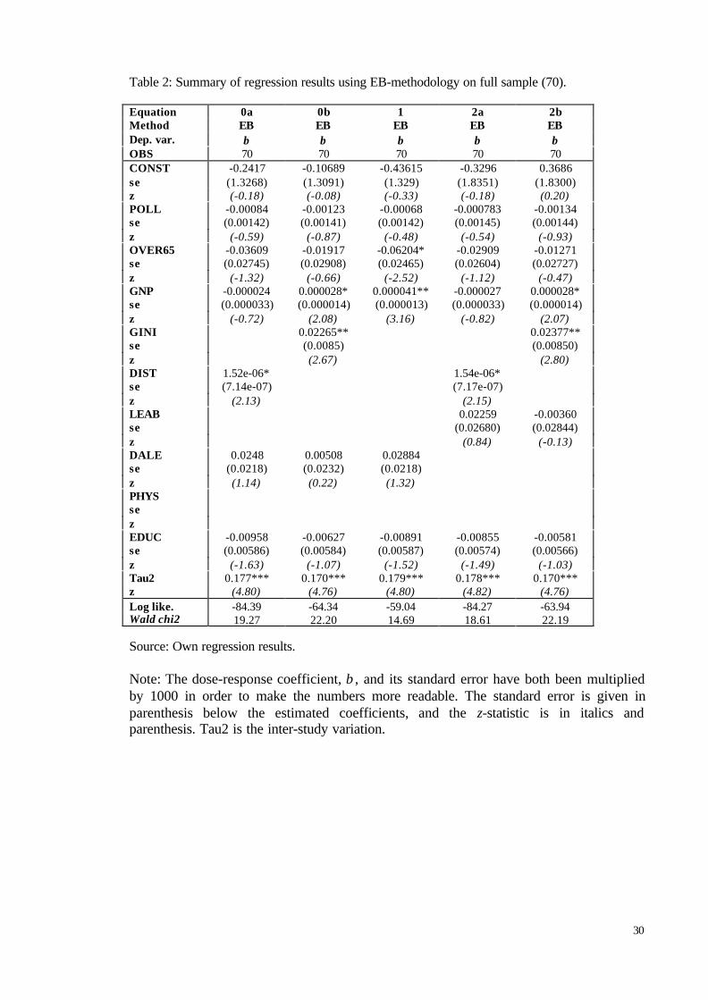
30
Table 2: Summary of regression results using EB-methodology on full sample (70).
Equation 0a 0b 1 2a 2bMethod EB EB EB EB EBDep. var. β β β β βOBS 70 70 70 70 70CONSTse
-0.2417(1.3268)
-0.10689(1.3091)
-0.43615(1.329)
-0.3296(1.8351)
0.3686(1.8300)
z (-0.18) (-0.08) (-0.33) (-0.18) (0.20)POLLse
-0.00084(0.00142)
-0.00123(0.00141)
-0.00068(0.00142)
-0.000783(0.00145)
-0.00134(0.00144)
z (-0.59) (-0.87) (-0.48) (-0.54) (-0.93)OVER65se
-0.03609(0.02745)
-0.01917(0.02908)
-0.06204*(0.02465)
-0.02909(0.02604)
-0.01271(0.02727)
z (-1.32) (-0.66) (-2.52) (-1.12) (-0.47)GNPse
-0.000024(0.000033)
0.000028*(0.000014)
0.000041**(0.000013)
-0.000027(0.000033)
0.000028*(0.000014)
z (-0.72) (2.08) (3.16) (-0.82) (2.07)GINIse
0.02265**(0.0085)
0.02377**(0.00850)
z (2.67) (2.80)DISTse
1.52e-06*(7.14e-07)
1.54e-06*(7.17e-07)
z (2.13) (2.15)LEABse
0.02259(0.02680)
-0.00360(0.02844)
z (0.84) (-0.13)DALEse
0.0248(0.0218)
0.00508(0.0232)
0.02884(0.0218)
z (1.14) (0.22) (1.32)PHYSsezEDUCse
-0.00958(0.00586)
-0.00627(0.00584)
-0.00891(0.00587)
-0.00855(0.00574)
-0.00581(0.00566)
z (-1.63) (-1.07) (-1.52) (-1.49) (-1.03)Tau2 0.177*** 0.170*** 0.179*** 0.178*** 0.170***z (4.80) (4.76) (4.80) (4.82) (4.76)Log like. -84.39 -64.34 -59.04 -84.27 -63.94Wald chi2 19.27 22.20 14.69 18.61 22.19
Source: Own regression results.
Note: The dose-response coefficient, β , and its standard error have both been multipliedby 1000 in order to make the numbers more readable. The standard error is given inparenthesis below the estimated coefficients, and the z-statistic is in italics andparenthesis. Tau2 is the inter-study variation.

31
Table 2 continued: Summary of regression results using EB-methodology (for full sample and sampleexcluding outlier (69)).
Equation 3a 3b 4a 4bMethod EB EB EB EBDep. var. β β β βOBS 69 69 70 (+ phys) 70 (+ phys)CONSTse
-0.2846(1.2352)
-0.12835(1.2173)
-0.44796(1.4429)
-0.2047(1.4295)
z (-0.23) (-0.11) (-0.31) (-0.14)POLLse
-0.000409(0.001323)
-0.00084(0.00131)
-0.00064(0.00153)
-0.00114(0.00154)
z (-0.31) (-0.64) (-0.42) (-0.74)OVER65se
-0.03758(0.02571)
-0.01903(0.02724)
-0.02997(0.03151)
-0.01651(0.03223)
z (-1.46) (-0.70) (-0.95) (-0.51)GNPse
-0.000032(0.000031)
0.000020(0.000013)
-0.000020(0.000034)
0.000028*(0.000014)
z (-1.04) (1.54) (-0.59) (2.05)GINIse
0.02356**(0.00793)
0.02213*(0.0091)
z (2.97) (2.42)DISTse
1.54e-06*(6.70e-07)
1.42e-06’(7.68e-07)
z (2.30) (1.85)LEABsezDALEse
0.01928(0.02034)
-0.00144(0.0216)
0.02756(0.02315)
0.00685(0.02527)
z (0.95) (-0.07) (1.19) (0.27)PHYSse
-0.03089(0.07765)
-0.01437(0.07688)
z (-0.40) (-0.19)EDUCse
-0.00385(0.00560)
-0.00046(0.00557)
-0.00947(0.00594)
-0.00634(0.00590)
z (-0.69) (-1.03) (-1.59) (-1.07)Tau2 0.148*** 0.141*** 0.182*** 0.176***z (4.80) (4.77) (4.80) (4.75)Log like. -73.96 -53.43 -88.74 -68.77Wald chi2 17.79 21.73 19.10 21.84
Source: Own regression results.
Note: The dose-response coefficient, β , and its standard error have both been multipliedby 1000 in order to make the numbers more readable. The standard error is given inparenthesis below the estimated coefficients, and the z-statistic is in italics andparenthesis. Tau2 is the inter-study variation.
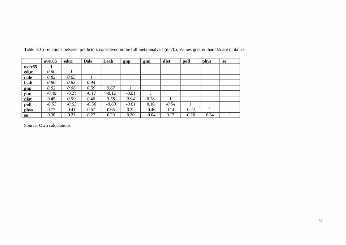
32
Table 3: Correlations between predictors considered in the full meta-analysis (n=70). Values greater than 0.5 are in italics.
over65 educ Dale Leab gnp gini dist poll phys seover65 1educ 0.60 1dale 0.82 0.65 1leab 0.80 0.63 0.94 1gnp 0.62 0.66 0.59 0.67 1gini -0.40 -0.21 -0.17 -0.12 -0.01 1dist 0.45 0.59 0.46 0.55 0.94 0.28 1poll -0.53 -0.63 -0.58 -0.63 -0.61 0.16 -0.54 1phys 0.77 0.41 0.67 0.66 0.32 -0.46 0.14 -0.22 1se 0.30 0.21 0.27 0.29 0.20 -0.04 0.17 -0.26 0.34 1
Source: Own calculations.

33
5.2 Sensitivity Analysis
There are several reasons why one should be very cautious when generalising the
results. First, the full sample is still relatively small, and single observations may affect
the results unduly. Second, the conversion factors used between different measures of air
pollution are approximations and may have affected the outcome. Also, there is a
possible difference in the ‘positive results’-bias between various countries. Furthermore,
both the mortality measures and the lag structure considered and/or reported vary
between the studies and may have induced errors. Finally, the fact that some of the
countries, as well as cities, in the study enter with multiple observations whereas others
have only one may be problematic and requires investigation. Given these drawbacks of
our sample, a sens itivity analysis is necessary before drawing conclusions about potential
causal predictors of the PM10-mortality relationship. Special attention is paid below to
outliers, mortality measure, negative results, lag structure, pollution measurement, and the
number of observations per location.
First, we undertook a search for outliers, i.e. subsets of the observations which, if
deleted, would change the results markedly, and tested the sensitivity of our results to
exclusion of these observations. When performing the DFITS-test (described in section
4.3) on our sample only Basel was singled out. From table 2 (equations 3a and 3b) we
observe two main changes in estimated effects when excluding Basel from the sample.
First, there is an increase in effect and significance of GINI and DIST in equations 3a and
3b, respectively. Second, a decrease in the positive effect of GNP occurs in equation 3b,
and an increase in the negative effect of GNP occurs in equation 3a. In both cases GNP is
insignificant. No observation in the sample failed Welsch’s Distance test.
Out of the sample of 70 pollution-mortality studies, 9 were not excluding mortality
due to external causes from their mortality measure. If externally caused mortality is
independent of air pollution, then including these studies in the full sample should not bias
the results – they would at most bring more noise into the results. However, to our
knowledge no study specifically investigates the association between accidents and
homicides etc. and air pollution.
When excluding studies measuring all-cause mortality, the central effect estimate is
5.9 per cent (CI: 5.0 – 6.8 per cent), whereas only looking at all-cause mortality studies
gives a mean of 6.5 per cent (CI: 0.13 – 1.18 per cent). Next, we tested whether the
inclusion of studies measuring all-cause mortality induced estimation errors using the two
main moderator effect models. In table 4 equation 5a we see that the main significant effect

34
of this exclusion was to increase the negative effect of GNP on the dose-response coefficient
– this coefficient becomes weakly significant at the 0.1 level – and increase the size and
significance of the interaction term, DIST. As for the other terms, their coefficients were
similar in magnitude and direction to the optimum model and remain insignificant. When
DIST is replaced by GINI (equation 5b), we observe that the increasing effect of GNP on
the dose-response coefficient found in the full sample regression decreased and became
insignificant through the exclusion of the 9 studies. The increasing effect of GINI on the
particle-mortality association, on the other hand, increased further. The remaining
coefficients remained insignificant, as compared to the full-sample model, and except for
CONSTANT and DALE the coefficients of the additional terms had the same sign.
Out of the pollution-mortality studies, 6 reported negative results, and 4 out of these
originated from the EMECAM program studies (i.e. Spain). If all confounding variables
were controlled for, the model correctly specified, and the data measured without error, it
seems unlikely that we would find negative estimates of the dose-response coefficient, i.e.
indicating that air pollution decreases mortality. Hence, we could view the studies reporting
negative coefficients as noise in our meta-analysis and therefore leave these out of the
analysis.20
The main objection against exclusion of negative results has to do with researcher-
induced sample-selection bias. The negative studies may to some extent counteract the noise
in positive studies, studies that we would not discard because they have the “right” sign.
Furthermore, it is highly likely that if all results had an equal chance of getting published
(i.e. without prejudices against negative results) we would in fact have had more negative
coefficients in our meta-analysis.
If we exclude the negative coefficients from our sample (hence, sample size 64), the
grand mean is 6.7 per cent (CI: 5.9 – 7.5 per cent). The findings from estimating the two
main models using the sample consisting only of positive results are similar to those we
obtained when we excluded all-cause mortality studies from the sample (equations 6a and
6b).
20 An additional, but rather tentative, reason for excluding the negative results is that 4 out of the 6 originatedfrom the EMECAM program studies (i.e. Spain). If all the countries in our analysis had an equal probability ofreporting and publishing negative results, then including these studies in the full sample should not affect therelative significance of the moderator variables. However, were this not to be the case, then the ‘positiveresults’-bias may influence our conclusions. Since Spain and the United States receive the most weight in themeta-analysis due to multiple observations for each country, it is worth noting that the US studies were allpublished in international and competitive journals, whereas the Spanish studies were both carried out due to agovernment grant and published in a government-supported journal. The ‘positive results’-bias may thereforewell have been larger in the US than in Spain, and for comparability of results one may hence argue that thenegative results should be excluded.
35
As mentioned in section 4.1, the correlation between the different particle measures
may have seasonal, meteorological, and geographical variations, and using fixed and
common conversion factors will most likely induce some measurement error.
The central effect estimates when stratifying by pollution measure were 5.0 per cent
(CI: 3.4 – 6.7 per cent), 6.6 per cent (CI: 5.1 – 8.2 per cent ), and 6.4 per cent (CI: 4.9 –
7.8 per cent), for BS, TSP, and PM10, respectively.21 We also tested the sensitivity of our
findings from the main models to the air particle measurements used, by considering the
coefficients derived using TSP, BS, and PM10 separately. A main cautionary remark is
called for before entering into the more specific challenges we are faced with when
analysing the samples stratified by pollution measurement. The sample sizes for each
pollution measurement is relatively small (24 observations for TSP, 33 in the case of
PM10, and 16 for the BS measurement), and any results have to be taken with the utmost
caution. As most of the moderator variables are country based, rather than city based, and
some (GINI and DALE) are available for a certain year only and not in time-series, the
regression model developed above is only meaningful when a variety of countries are
included in the sample. Furthermore, the larger the amount of studies in the sample
originating from the same country, the more likely it is that the variables that do vary from
one study to the next proxy for those that do not. Keeping this in mind, and given that 50 per
cent of the studies using BS to measure air pollution are from Spain and approximately 50
per cent of those using PM10 have been carried out in the US, we argue that the results from
these two samples will not be very meaningful. In the case of the sample of 24 TSP based
coefficients, 13 countries are represented and none with more than 5 coefficients. Equations
7a and 7b of table 4 give the results of the main model for the TSP-sample. When we
compare the results with those of the full sample for the model which includes DIST, we
observe a strengthening of the negative effect of GNP on the dose-response coefficient,
although it remains insignificant. Furthermore, the size and significance of the interaction
term increases. The remaining coefficients once more remain insignificant, however only
EDUC which was close to being significant in the full sample retains the direction of its
coefficient. With GINI replacing DIST (equation 7b), we observe that the positive effect of
GNP on the dose-response coefficient found in the full sample regression decreases and
becomes insignificant. The positive effect of GINI on the particle-mortality association, on
the other hand, increases further. The remaining coefficients once more remain insignificant,
21 The sample sizes for the three air pollution measures estimates were 16, 24, and 33 for BS, TSP and PM10
(including two studies using PM13), respectively. The sample adds up to more than our full sample because3 of the studies reported estimates in two of the measures.
36
and only the coefficients for POLL and EDUC do not change direction. For the sake of
completeness the results of the main model for the PM10 and BS-sample are given in
equations 8 and 9 (table 4), respectively.
Next, we investigated the sensitivity of our findings to the choice of lag structure. In
particular, we ran our favoured model on samples of the pollution-mortality coefficients that
were obtained for average air particle levels of the same day (table 5, equations 10a and
10b), previous day (table 5, equations 11a and 11b), and of two days previously (lag 2 –
equations 12a and 12b) in turn. Before proceeding, however, the same warning has to be
made as was made in connection with the pollution measurements analysis on the
previous page. The sample sizes for each lag is relatively small (28 observations for lag
1, 23 in the case of lag 1, and 12 for lag 2), and any results have to be taken with the
utmost caution, and in particular in the case of the smaller samples is likely to drive the
results. Interestingly, the results varied widely. For same day air pollution, the GINI
coefficient was once again found to have a strongly significant 22 positive effect on the dose-
response coefficient, whereas GNP took a negative sign but was insignificant. POLL has a
significantly negative effect on the relationship. As for baseline health, it is found to have an
increasing and significant effect, whereas education has a decreasing and significant effect.
For particle pollution lagged one day, none of the moderator terms have significant
coefficients. In the case of two-day lagged pollution, however, GINI is once again weakly
significant,23 with the usual positive sign, and the coefficient for education is significant and
this time takes a positive sign. The estimates of central effect were 5.3 per cent (CI: 4.3 – 6.2
per cent), 5.5 per cent (CI: 4.1 – 6.9 per cent), and 3.7 percentage (CI: 1.6 – 5.7 per cent) for
lag 0, lag 1, and lag 2, respectively.24
Furthermore, we tested the sensitivity of our findings to the decision to include
several studies from the same city, in order to detect the potential effects of double counting.
Only 5 cities have been entered twice in the sample, and we tested several combinations
when only one of these studies was considered (sample size was then 65). As expected,
the findings did not change significantly from those made for the full sample.
If we had obtained information on the values of the moderator variables at the city
level, rather than at the country level, the fact that some countries enter with several
observations whereas others only with one would not have been a cause for concern.
However, this is not the case – only the average particulate measure was based on the exact
22 The null-hypothesis of no effect is rejected at the 0.1 per cent level.23 The null-hypothesis of no effect rejected at the 10 per cent level, but not at the 5 per cent level.24 The sample sizes for lag 0, 1, and 2 were 28, 23, and 12, respectively.

37
study location. Our final sensitivity test therefore consisted of including only one
observation for each country. This can be done in three alternative ways. First, the variance
weighted averages of both the dependent and independent variables, as well as of the
standard error, are calculated for those countries with more than one observation, and the
resulting averages can then be entered as observations for those countries. The second
procedure is an extension of the first; the only difference is that we take the time period in
which the studies were carried out into account, since we have time series data for most of
the moderator variables. All studies from one country carried out mainly in the period 1975-
85 were averaged, as were those for the periods 1985-95, and 1995-, implying that we had
two “observations” each for Spain and Germany, and three for the US, and thus a sample of
25. Finally, we can consider only one (real) study per city, and a number of potential study
combinations.
The two main regressions were performed on the simple country-averaged sample of
21 observations (table 6, equations 13a and 13b) and on the period sensitive country-
averaged sample of 25 observations (table 6, equations 14a and 14b). The results from the
two samples were similar to each other, and significantly different from our previous results.
Once again, however, a cautionary remark is in order when interpreting the results, due to
the sample sizes. Both education (EDUC) and the amount of older people in the population
(OVER65) were found to have significantly negative effects on the dose-response
coefficient, i.e. higher levels of these variables are associated with lower PM10-mortality
coefficients. As for the two income distribution terms, they were both insignificant when
entered in turn. When entered together with the relative income inequality measure, GINI,
the average income-term takes a positive coefficient and is highly significant. As for the
income coefficient when the interaction term, DIST, is included in the model, GNP has a
significantly positive coefficient in the sample of 21 observations, but is insignificant in the
sample of 25. The estimates of the central effect is 4.9 per cent (CI: 3.9 – 5.9 per cent) in the
sample with 21 observations, and 5.0 per cent (CI: 4.1 – 6.0 per cent) in the sample
consisting of 25.25
With over 2 million potential study combinations, a complete combination analysis
was not deemed feasible. However, by randomly selecting 24 combinations and performing
the two main regressions, we propose that we can gain some insights from which we can
generalise.26 Focussing first on the model including the GINI term, we found that GNP
entered the regression significantly for 54 per cent of the study combinations, with a
25 When including only one observation for each country, the sample size is 21.26 Refer to appendix F for the regression results.
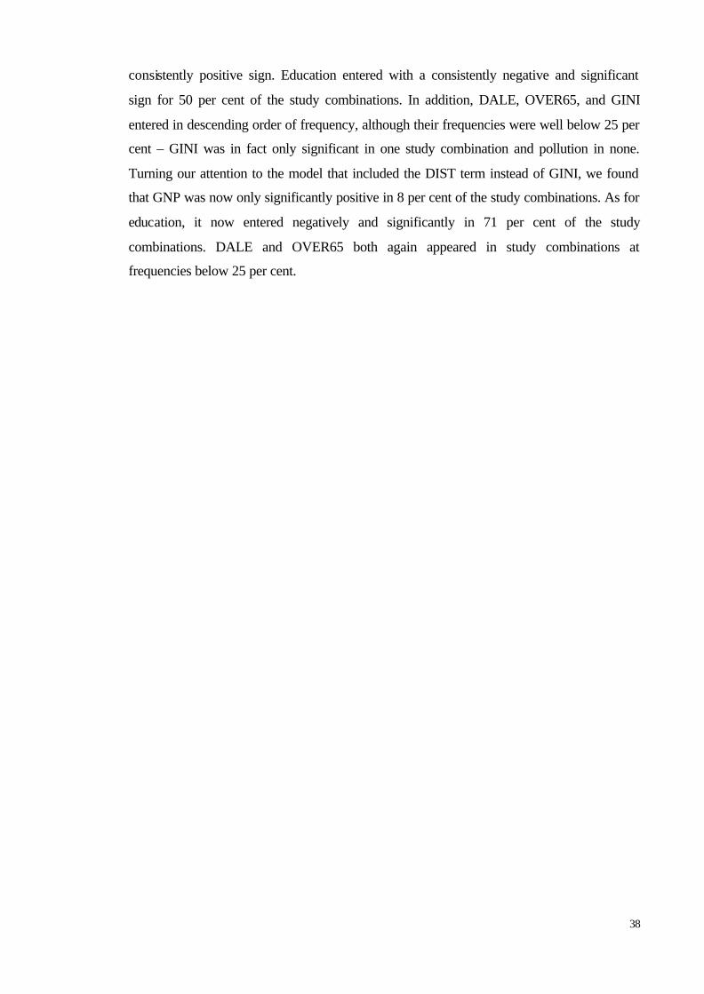
38
consistently positive sign. Education entered with a consistently negative and significant
sign for 50 per cent of the study combinations. In addition, DALE, OVER65, and GINI
entered in descending order of frequency, although their frequencies were well below 25 per
cent – GINI was in fact only significant in one study combination and pollution in none.
Turning our attention to the model that included the DIST term instead of GINI, we found
that GNP was now only significantly positive in 8 per cent of the study combinations. As for
education, it now entered negatively and significantly in 71 per cent of the study
combinations. DALE and OVER65 both again appeared in study combinations at
frequencies below 25 per cent.
39
Table 4: Summary of regression results using EB-methodology (sample excluding all-cause mortality studies (61), sample excluding negative coefficients (64),sample of TSP studies (24), PM10 studies (33), and BS studies (16)).Equation 5a 5b 6a 6b 7a 7b 8 9Method EB EB EB EB EB EB EB EBDep. var. β β β β β β β βOBS 61 (- accid) 61 (-accid) 64 (- neg) 64 (-neg) 24 (TSP) 24 (TSP) 33 (PM10) 16 (BS)CONSTANT(se)
-0.0101(1.2239)
0.2070(1.1940)
-0.4408(1.1066)
-0.2518(1.0770)
0.7019(2.8333)
0.2659(2.9177)
-1.2173(3.1341)
-4.6017(3.1584)
(-0.01) (0.17) (-0.40) (-0.23) (0.25) (0.09) (-0.39) (-1.46)POLL(se)
-0.00090(0.00131)
-0.00149(0.00129)
-0.00114(0.00120)
-0.00162(0.00118)
0.00146(0.00459)
-0.000275(0.00473)
-0.00119(0.00357)
-0.00490’(0.00267)
(-0.69) (-1.16) (-0.95) (-1.38) (0.32) (-0.06) (-0.33) (-1.83)OVER65(se)
-0.02539(0.02654)
-0.00437(0.02766)
-0.01352(0.02493)
0.00865(0.02612)
0.00495(0.05099)
0.01425(0.05487)
-0.16550***(0.04911)
-0.08868(0.20868)
(-0.96) (-0.16) (-0.54) (0.33) (0.10) (0.26) (-3.37) (-0.43)GNP(se)
-0.0000559’(0.0000317)
0.0000149(0.0000129)
-0.0000395’(0.0000287)
0.0000135(0.0000117)
-0.000075(0.000062)
0.000052(0.000046)
0.000079***(0.000021)
0.000178(0.000116)
(-1.76) (1.15) (-1.38) (1.15) (-1.21) (1.14) (3.75) (1.54)GINI(se)
0.03044***(0.0081)
0.02539***(0.00723)
0.03857*(0.01787)
0.01531(0.01568)
-0.15899(0.10366)
(3.76) (3.51) (2.16) (0.98) (-1.53)DIST(se)
2.08e-06**(6.91e-07)
1.60e-06**(6.25e-07)
4.24e-06**(1.56e-06)
(3.00) (2.56) (2.72)DALE(se)
0.01558(0.02062)
-0.01075(0.02172)
0.02333(0.01817)
0.00064(0.01911)
-0.00991(0.03397)
-0.02397(0.03906)
0.0393(0.05042)
0.17084(0.11149)
(0.76) (0.50) (1.28) (0.03) (-0.29) (-0.61) (0.78) (1.53)EDUC(se)
-0.00437(0.00598)
-0.000197(0.00585)
-0.00604(0.00511)
-0.00247(0.00499)
-0.00366(0.0149)
-0.000474(0.0156)
-0.00912(0.00931)
-0.02883(0.03062)
(-0.73) (-0.03) (-1.18) (-0.50) (-0.25) (-0.03) (-0.98) (-0.94)Tau2 0.136*** 0.127*** 0.110*** 0.101*** 0.257** 0.278** 0.158** 2.10e-13
(4.52) (4.44) (4.45) (4.39) (2.80) (2.78) (2.84) (0.00)Log like. -67.41 -46.28 -59.21 -37.68 -78.23 -60.82 -56.92 -28.95Wald chi2 20.84 26.57 21.16 27.52 11.95 9.09 29.86 64.83‘P<0.1, *P<0.05, **P<0.01, ***P<0.001, β and se have both been multiplied by 1000.

40
Table 5: Summary of regression results using EB-methodology (sample of lag 0 coefficients (28), lag 1 coefficients (23), and lag 2 coefficients (12).
Equation 10a 10b 11a 11b 12a 12bMethod EB EB EB EB EB EBDep. var. β β β β β βOBS 28 (lag 0) 28 (lag 0) 23 (lag 1) 23 (lag 1) 12 (lag 2) 12 (lag 2)CONSTANT(se)
-3.0395’(1.5626)
-2.8248*(1.2782)
-3.2315(3.7424)
-3.0477(3.7276)
6.8799(5.8035)
3.4584(4.7874)
(-1.95) (-2.21) (-0.86) (-0.82) (1.19) (0.72)POLL(se)
-0.00426**(0.00159)
-0.00475***(0.00136)
0.00011(0.00392)
0.00055(0.00399)
-0.00871(0.00573)
-0.00795(0.00533)
(-2.69) (-3.50) (0.03) (0.14) (-1.52) (-1.49)OVER65(se)
-0.00072(0.03982)
0.01920(0.03066)
0.00888(0.07217)
0.02318(0.07606)
0.00673(0.18719)
-0.04446(0.16149)
(-0.02) (0.63) (0.12) (0.31) (0.04) (-0.28)GNP(se)
-0.000108*(0.000045)
-1.63e-06(0.000011)
1.64e-07(0.000053)
-8.55e-06(0.000027)
-0.000199(0.000153)
-0.000035(0.000056)
(-2.38) (-0.14) (0.00) (-0.32) (-1.31) (-0.63)GINI(se)
0.035780***(0.00685)
0.00545(0.01677)
0.0760’(0.04355)
(5.23) (0.33) (1.75)DIST(se)
2.83e-06**(9.05e-07)
-1.64e-07(1.21e-06)
5.23e-06(3.19e-06)
(3.13) (-0.14) (1.64)DALE(se)
0.07652**(0.02880)
0.04667*(0.02205)
0.04342(0.07168)
0.03390(0.07431)
-0.10986(0.10606)
-0.11412(0.10456)
(2.66) (2.12) (0.61) (0.46) (-1.04) (-1.09)EDUC(se)
-0.01663*(0.00737)
-0.01331*(0.00565)
0.00784(0.01033)
0.00944(0.01113)
0.0220(0.01724)
0.04462*(0.02219)
(-2.26) (-2.36) (0.76) (0.85) (1.28) (2.01)Tau2 0.1625 9.42e-16 0.1558** 0.1580** 0.191 0.179
(1.08) (0.00) (2.58) (2.59) (1.29) (1.28)Log like. -61.71 -37.71 -68.44 -49.34 -69.91 -50.62Wald chi2 27.00 51.13 8.94 8.94 10.91 11.67‘P<0.1, *P<0.05, **P<0.01, ***P<0.001, β and se have both been multiplied by 1000.

41
Table 6: Summary of regression results using EB-methodology (sample consisting of one coefficient (averaged or actual) per country (21), and taking time-periodinto account (25)).Equation 13a 13b 14a 14bMethod EB EB EB EBDep. var. β β β βOBS 21 (country) 21 (country) 25 (country) 25 (country)CONSTANT(se)
-0.3806(1.2077)
-0.3244(1.2440)
-0.5841(1.1836)
-0.5168(1.1926)
(-0.32) (-0.26) (-0.49) (-0.43)POLL(se)
0.00129(0.00158)
0.00149(0.00156)
0.00065(0.00144)
0.00052(0.00145)
(0.82) (0.95) (0.45) (0.36)OVER65(se)
-0.0654*(0.0293)
-0.0598’(0.0335)
-0.0570*(0.02832)
-0.0518’0.0313)
(-2.23) (-1.79) (-2.02) (-1.65)GNP(se)
0.000072*(0.000033)
0.000059**(0.000022)
0.000028(0.000033)
0.000042**(0.000016)
(2.18) (2.64) (0.85) (2.62)GINI(se)
-0.000072(0.00860)
0.00583(0.00874)
(-0.01) (0.67)DIST(se)
-4.00e-07(7.56e-07)
4.15e-07(7.50e-07)
(-0.53) (0.55)DALE(se)
0.03015(0.02062)
0.02779(0.02426)
0.03107(0.01988)
0.02508(0.02312)
(1.46) (1.09) (1.56) (1.09)EDUC(se)
-0.01579**(0.00601)
-0.01549*(0.00641)
-0.01191*(0.00585)
-0.01076’(0.00618)
(-2.62) (-2.42) (-2.04) (-1.74)Tau2 0.0666* 0.0698* 0.0667** 0.0662**
(2.37) (2.47) (2.75) (2.75)Log like. -59.52 -41.00 -56.47 -37.66Wald chi2 14.66 14.02 14.33 14.51
42
5.3 Discussion
Given the sensitivity of the findings to the sample choice and the measures used,
interpretation is a challenging task. In this section we will first discuss the general
findings from regressions carried out on the full sample (sample size 70), the sample
excluding the 9 all-cause mortality studies (sample size 61), as well as on the sample
consisting of coefficients derived using the TSP measure of particles (sample size 24).
We will then compare and contrast these results with those obtained with the samples
stratified according to the particle measure and the lag structure, as well as with those that
include only one observation (an actual observation or an averaged one) for each country.
Among the moderator variables tested, GINI and the interaction term DIST are
the strongest and most stable predictors of the dose-response relationship. The positive
coefficients indicate that higher income inequality in general, as measured by the GINI-
coefficient, and in high-income countries in particular, as captured by the interaction term
DIST, are associated with higher mortality rates from air particles.
The GINI-model yielded a positive coefficient for the GNP term, however, it is
only significant in the full sample. In the case of the DIST-model, the GNP term takes a
negative coefficient that is weakly significant only in the case of the sample excluding the
all-cause mortality studies. This main tendency suggests that the negative direct effect of
income is smaller than the indirect increasing effect via its interaction with income
inequality. In other words, the effect income has in increasing the positive effect of the
inequality in income distribution on the dose-response coefficient is larger than the
negative (decreasing) effect of average income on the PM10-mortality association.
In section 3 we mentioned four possible reasons for income inequality to have an
increasing effect on the mortality rate from air pollution. Fist, decreasing returns to
averting and mitigating activities would imply a tendency for higher inequality to be
associated with higher mortality rates from changes in air pollution levels. Second, if
individuals with relatively low income live in the most polluted areas, and if the adverse
effect of air pollution is larger on lower income individuals, then this would once again
imply larger PM10-mortality in cities with large income inequality. Third, if mortality is
associated with stress, and stress is related to social status, then higher income inequality
may lead to a larger mortality rate from air pollution. Finally, GINI may have been
proxying for inequalities in baseline health or for the quality and availability of health
care. We did include health services as a moderator variable in one of our regression
models, and found a slight decrease in the significance for both GINI and DIST, however,
43
both remained significant. Since our measure of health services was relatively poor,
however, this does not necessarily imply that GINI is not proxying for some aspect of health
services.
Our findings provide empirical support for the idea that income inequality has an
increasing effect on the mortality rate from air pollution. However, with the level of
aggregation of our data there is little we can do in terms of choosing among the above
explanations.
One implication of the regression results for income level and inequality (as
captured in the variable DIST) is rather surprising: inequality in income has a larger
positive effect on the PM10-mortality association in high-income countries. At the risk of
‘over-interpreting’, two explanations may be given for this phenomenon. First of all,
there may be more mitigating and averting activities available in high-income countries
to the ones who can afford it. The idea is that the supply side of health investments is
more developed in high-income countries, e.g. the existence of low pollution
neighbourhoods, well-isolated houses, air filtering systems, medicines, medical advice,
high-quality medical procedures. In addition, and related to this, comes the fact that the
awareness of the general population, irrespective of income level, about the health risks
from air pollution and how to minimise them probably is higher in high-income
countries. The second possible explanation for the positive sign of the GNP and GINI
interaction term is that high income inequality leads to more psychological stress in a
high-income country than in a country with a lower level of average income, or
alternatively that the stress induced by inequality is more fatal. First, the higher level of
stress may be related to various media incessantly informing and reminding people of the
differences. Second, different life-styles (diet, exercise etc.) may mean that stress has a
more fatal outcome in high-income countries. Furthermore, high-income countries also
tend to have a higher degree of social mobility, something which possibly affects the
stress-level experienced by ‘under-achievers’. Finally, there is possibly a stronger focus
on material status in high-income countries.
Another slightly surprising finding is the very small and insignificant direct
negative effect of income on the dose-response coefficient. It is possible that income does
not affect behaviour (averting and mitigating activities) to such an extent that it shows up
very significantly in the regression results. Income level is likely to affect the level of
baseline health and education, however these are measured by other moderator variables.
A very likely, and perhaps more plausible explanation, however, of the lack of
significance of the coefficient for the direct effect of income, is that it is highly correlated

44
with education, disability-adjusted life expectancy, the percentage of the population over
65 years of age, and the ambient level of pollution (see table 2). As long as the measures
used are not perfect, income may be picking up parts of these effects, some of which
work in opposing directions. Alternatively, the other measures may have captured part of
the effect that should have been captured by income.
We should also remind the reader that the income variable we ideally would like
to have is the average income in the location in question (and preferably of the population
particularly vulnerable to air pollution). Since we were not able to obtain this
information, we had to use the average income in the relevant country instead. Not only
may this imply that our income measure is fairly poor, but in addition it may imply that
the GINI coefficient partly proxies for the city income-level.
As for the additional moderator variables POLL, OVER65, EDUC, DALE, and
the constant, none was significant in any of the three samples mentioned. The education
term was the most consistent of these variables, taking a negative coefficient in all of the
samples. The sign suggests that the amount of knowledge or education people have may
play a role in avoiding fatal effects from air pollution.
The effect of the average ambient level of pollution (POLL) on the PM10-
mortality coefficient varies in sign and is insignificant. This finding suggests that non-
linearities in the effect of particles on mortality are not very significant. The positive but
insignificant coefficient for ambient PM10 concentration found in Levy et al. (2000) is in
line with our finding.
Similarly, the coefficient for baseline health (DALE) varies in sign from one
sample and regression model to another, but it is consistently insignificant. Again, this
could indicate that basic health level does not affect significantly the rate at which people
die from air pollution. In principle, it is possible that a healthy person could die suddenly
from high exposure to air pollution, just as well as an older person or a person suffering
from some illness, however, this does not make sense intuitively. The insignificance of
the coefficient is most likely due to DALE not being a satisfactory measure of baseline
health.
The coefficient for percentage of the population over 65 years of age also varies
in sign according to the sample we are analysing, but is consistently insignificant. Only
when we excluded any measure of income inequality from our regression equation did
OVER65 become significantly negative, something which suggests that it was proxying
for income inequality (from table 3 we observe that the correlation is –0.40). Levy et al.
(2000) found a negative and weakly significant coefficient for population over 65 years
45
of age (per cent) in their regression analysis on a sample of 19 U.S. studies. The
difference in results between the two studies may possibly be explained by the fact that
this latter study did not include income inequality or baseline health as moderator
variables in their regressions.
In section 4 we argued that we would expect elderly people to be most at risk
from the acute effects of air pollution, and therefore a positive coefficient for this
moderator variable. So how do we explain these findings? We suggest that since baseline
health is such a multi-faceted concept, no single moderator variable will adequately be
able to measure the desired dimension. It is therefore possible that, although we have
included DALE as a measure of baseline health in our regression model, OVER65 is still
picking up part of the effect of higher baseline health on the PM10-mortality association.
The reason for this is that individuals tend to survive to a high age if they are in good
health, so a society with a large proportion of elderly people may also be a “healthy”
society. This will then induce a downward bias in the estimator, which may have
cancelled out the expected positive coefficient for OVER65.
The inclusion of a number of moderator variables is required in order to
distinguish among potential predictors. However, the lack of independence can pose
problems. The findings discussed above of insignificant coefficients, with varying signs,
for DALE, OVER65, and POLL may be a function of these correlations. In addition,
these moderator variables may not be measuring the desired dimensions or may not
represent the actual characteristics of the site. Both DALE and OVER65 are based on
country data, rather than data from the site in question. In addition, DALE exists for one
year only, and may therefore be very misleading especially in the case of older studies.
Although pollution data are available for the particular city we are studying, potentially
significant information e.g. on pollutant mixture and particle size was missing.
Interestingly, we find that the estimate of the central effect of PM10 on mortality is
larger when studies of all-cause mortality are included rather than excluded from the sample.
As the three types of particulate pollution measures are all represented in the 9 studies
investigating all-cause mortality, the type of particulate measure used is unlikely to have
caused this difference in results. Although the 9 studies may differ from the rest of the
sample in some other unidentified way, it is also possible that externally caused mortality is
not entirely independent of air pollution. In particular, we suggest that air pollution may
affect individuals’ level of concentration, stress, as well as visibility and that therefore the
amount of externally induced mortality incidences increases with higher levels of air
46
pollution. Furthermore, air pollution will tend to be correlated with the amount of traffic,
and thereby possibly with traffic-accidents.
By stratifying the sample according to the particle measure, we observed that the
particle measure used affected the findings on the PM10-mortality association. Although
erroneous conversion factors can explain the differences in central effect estimates
according to the pollution measure used, they cannot explain the extent to which the
estimated moderator-effects and their significance differ. The fact that most of the
moderators are country based means that regressing the observed dose-response coefficients
on these variables only makes sense when a variety of countries are included in the sample.
Since half of the selected studies using BS to measure air pollution are from Spain and half
of those using PM10 have been carried out in the US, we argued that the results from these
two samples would not be meaningful. For the record, it is worth mentioning that even with
samples where such a moderator-effect analysis is meaningful, differences in moderator
effects could nevertheless be expected. The studies using BS are likely to differ from those
employing PM10 in several important respects. First of all, BS is a measure based on older
technology and is therefore typically used in earlier air pollution studies. Second, PM10
became a commonly used measure of air particles in the US before most other countries,
and there is therefore a disproportionate amount of US studies in our sample that use this
measure. US studies, as well as newer studies may differ in several respects from older
studies and studies carried out in other countries (e.g. in terms of pollutant mixtures, and
population characteristics), and this could well be reflected in the moderator coefficients.
Two of the sensitivity tests undertaken in this paper stand out from the rest
because of the very different results from those discussed above; the test for sensitivity to
the lag structure, and that for the sensitivity to multiple observations for some countries.
We will discuss the main findings from these analyses in turn and consider whether they
are seriously challenging the results from the rest of the regression analysis.
The results from regressing the dose-response coefficients on the moderator
variables varied widely according to the time lag of the pollution measurement used in
the original study. For the association between same-day air pollution and mortality we
found that the GNP coefficient is significantly negative and the DIST-coefficient
significantly positive. When GINI is included instead of DIST, GNP retains the negative
sign but is insignificant. These results are in line with our previous findings. However,
for air pollution lagged one day there is no significant effect from income, income
inequality, or their interaction term. In the case of a two-day lag, the effects are similar to
47
the same-day effects for the income-related variables but the significance levels are
lower, and only GINI is weakly significant.
The widely varying results according to the lag structure are most likely due to the
small sample sizes. The sample for lag zero consists of 28 observations, for lag one 23,
and in the case of lag two, 12. One has to be extremely cautious with results based on
small sample sizes, and in particular in the case of the smaller samples, i.e. lag one and
two, the size of the samples is likely to drive the results. The smaller the size, the wider
the confidence interval, reflecting an amount of uncertainty about the parameter being
estimated, which becomes undesirable at some point. Everything else equal, the results
from the analysis upon the largest sample are more likely to have some meaning,
although caution is still required. These results were nevertheless found to be in line with
our previous findings.
If we have included the main explanatory variables in our regression model, then
the representativeness of the sample would not have been an issue. The reason for this is
that the requirement for a sample to be representative is based on the idea that there may
be underlying factors not known or fully understood by the researcher that influence the
relationship under investigation. If, however, the moderators cannot adequately account
for the discrepancies between study findings, then the fact that the sample may be
unrepresentative constitutes a challenge. How serious this challenge is depends to some
extent on what we would like to do with our findings. In particular, the challenge will be
present if we would like to generalise our results in order to tailor-make dose-response
coefficients to different circumstances. If, on the other hand, the purpose of the meta-
analysis is first and foremost the wish to investigate whether various variables are
significantly affecting the PM10-mortality ratio, rather than the actual size of the effect,
the unrepresentativeness of the sample may not be such a problem.
It is, however, not straightforward to determine what would have been a
representative sample – ‘the concept of representativeness has always been a somewhat
ambiguous idea, but the concept is useful in helping to illuminate potential problems in
drawing inferences from samples’ (Cooper and Hedges (1994), p. 35). Like Levy et al.
(2000), we assume that the studies are independent samples from a random distribution of
the conceivable population of studies. The latter being all the potential studies that could
have been carried out given our inclusion and exclusion criteria. This assumption is
clearly difficult to support, mainly due to the overweighing of certain countries and cities,
but also due to the sample entailing multiple studies conducted by the same author(s) and
using the same methodology. On a more general note, there are two main reasons why
48
exhaustiveness of sampling does not necessarily yield a representative sample of the
universe. First, some types of studies in the intended universe may not have been
conducted (e.g. because of unreliable data), and second, although studies may have been
conducted, they may not have been reported in journals or other forums accessible to the
researcher.
To determine whether the results were sensitive to study selection, and in
particular to the inclusion of multiple observations from certain countries, we therefore
conducted analyses where each country entered with only one observation, either an
averaged one or from one single study (randomly chosen). Averaging the data over
several studies, and using the average as if it were an observation is a very dubious
method, and is likely to create correlations between variables where these do not exist.
These problems are worsened in the case where the averaged data came from studies
covering very different time periods. Including single studies is therefore a preferred
method when testing the sensitivity to multiple country observations. The main
objections to this latter method are, first, that the sample becomes smaller, second, that
we are ignoring/rejecting information that we actually have, third, that the observation
that happen to be included may be unrepresentative for the country in question, and
finally, the resulting sample may not necessarily be more representative than the full
sample. Compared to the results from the full study, this country-weighted sensitivity
analysis found a more significant effect of education in decreasing the particle-mortality
effect. Furthermore, no significant role was found for either the GINI-coefficient or its
interaction term with GNP. The role of income appears relatively unchanged, with a
positive and significant effect in the GINI-model, and no significant effect in the DIST-
model. These findings are similar to those obtained on the sample where data for the
same country, of the same time-period, were averaged.
When comparing the result using the full sample with those using the ‘one-
country-one-observation’ sample, the differences in results are of degree rather than of
tendency/direction. The coefficient for education is consistently negative, for income
inequality it is consistently positive, and as for income, it tends to have a direct effect
which is either negative or zero, and an indirect effect via income inequality which is
positive. Significance varies between the samples.
We have seen that there are weaknesses related to both samples. We nevertheless
propose that the results based on the full sample are the preferred ones, since the sample
with one observation for each country excluded existing information without necessarily
49
becoming more representative of the universe of potential studies (given our selection
criteria).
Since the inter-study variability remained significant, it is quite likely that we
omitted relevant moderators that could have explained at least part of it. It is also possible
that omitted relevant moderators can explain the significance of some of the associations
we found, e.g. of income inequality. Possible omitted relevant explanatory variables are
smoking habits, the ratio of fine to coarse particles, other pollutants, central air
conditioning prevalence, and cooking and heating mechanisms used. Furthermore, the
data used to capture the moderator variables may have been poorly suited for that
purpose. Most of the data were given on a country-wide level, whereas the studies were
carried out for a specific region or city within that country which may well differ
significantly from the country-average with respect to that particular characteristics. In
addition, some of the moderator concepts were too complicated and vague to be captured
by one type of indicators, e.g. health services.
Even if the above weaknesses could be solved, the problem of selection bias
remains. Although we included all the available studies that fulfilled the selection criteria
set out in section 4, there is no way of avoiding possible “publication-bias” or
“submission-bias” (i.e. studies that do not find a significant relationship between PM10
and mortality, or that find a negative association, are not published or submitted for
publication). Nevertheless, the file-drawer bias is highly unlikely to change the finding of
a significant PM10-mortality link. With the assembled sample (70) of largely positive
estimates, 70 unpublished estimates with central estimates of –0.5 per cent and the mean
variance of our 70 study estimates would be required to yield a statistically insignificant
grand mean estimate. A further source of selection bias lies in the representativeness of
our study locations. As argued earlier, it is possible that the cities in our analysis are not
representative of the true range of conceivable studies. As argued by Levy et al. (2000), it
is possible that a subset of cities “that were more or less prone to PM health effects were
chosen for epidemiologic analyses” (p.115). The main problem with this challenge to our
sample is to know the range of conceivable studies. Nevertheless, the cities and countries
included in our sample represent a wide range of population characteristics and pollution
concentration levels.
One particular and potentially important weakness of the original studies may
have influenced the various findings from our meta-analysis. As briefly mentioned
towards the end of section 4.1, measuring PM10 exposure with readings of ambient
pollution from central monitoring stations may be highly problematic, especially in the
50
case of developing countries. If indoor air pollution in developing countries, caused by
the use of highly polluting heating and cooking fuels and little ventilation, is a larger
health risk than outdoor air pollution, then the exposure-response association may be
much larger but not be revealed by studies using exposure measurements obtained from
central monitoring stations. The individuals vulnerable to outdoor air pollution may
already have died from indoor air pollution, and the coefficient will not capture these
deaths adequately as long as indoor and outdoor air pollution do not strongly covary. A
possible implication of this measurement error is that those moderator variables that tend
to take a significantly different value in the case of developing than developed countries,
i.e. income per capita, education, and disability-adjusted life expectancy may have lost
significance.
A number of more general weaknesses and limitations to our meta-analysis are
necessary to point out. First of all, it is important to note that as the meta-analysis uses a
correlational design for its moderator variables, no causal inference can appropriately be
made. Secondly, when the moderator variables cannot adequately account for the
discrepancies between study findings, as is the case for our full sample, it becomes
unclear whether the various research operations represent a common underlying
construct, and uncertainty in the empirical effects of the moderators emerges.
Furthermore, unresolved inconsistencies between studies may compromise the ability to
detect true relations among variables. ‘In such cases’ states Cooper and Hedges (1994)
‘meta-analytic findings should be accorded relatively low certainty’ (p.490). Thirdly,
even if the moderator variables successfully account for the empirical variability in study
outcomes, the proper interpretation of the relation may remain an issue, especially when
the moderators are identified on a between-study basis. The moderator is then an attribute
of an entire study, and individuals in the primary research have not been randomly
assigned to levels of the moderator variable. Such moderator variables may be
confounded with other variables that covary with it.
Our first study-objective was to increase our understanding of what affects the
amount of deaths that are related to air pollution. From our regression results we have seen
that several of the population characteristics included as moderator variables may play a
significant role in the association between particle pollution and mortality. In particular,
income inequality may be associated with a larger effect of a change in pollution on the
mortality rate, especially in high-income countries. The direct effect of income may be
slightly decreasing the effect of pollution on mortality, and a similar finding was made for
education.

51
Second study-objective was to help highlight areas where further studies may be
needed. Indeed, we have pointed out that the discrepancies between study effects remain
significant, that some of the data are not very well-suited to capture the moderator effects in
question, that no causal inferences can appropriately be made for the moderator variables,
that the sample of studies may not be representative of the hypothetical universe of studies,
and that there may be serious measurement errors in the original studies. Subsequent
research will need to address all of these concerns. The first point can be addressed by
adding other possible moderator variables that have been discussed in the literature (e.g. the
ratio of fine to coarse particles, other pollutants, gas stove prevalence, central air
conditioning prevalence, warm air heating prevalence, smoking habits) to the ones
discussed in the present paper. This may not only eliminate the discrepancies between
study-effects, but may also alter the findings on the already included moderators. The
second point can be approached by for example trying to obtain city- or location-specific
information on the relevant moderator variables, and by more generally encouraging the
primary studies to gather and publish this information. Meta-analysts should also be on
the lookout for improved indicators of the moderator effects. In order to be able to make
causal inferences, the third point, two criteria in addition to covariance have to be
fulfilled; temporal ordering (i.e. that the cause should temporally precede the effect) and
isolation (that the effect was not caused by something else). This suggests that future
PM10-mortality research could be directed towards panel-studies gathering individualised
time-series data on the relevant moderator variables. As for the latter two points, future
primary research would benefit from being directed towards the understudied
populations; in particular, more studies from poor countries are required, and would also
benefit from improved exposure measurements; in particular, including indoor air
pollution exposure.
Final study-objective was, through the ensuing coefficients of the moderator
variables, to help transferring the dose-response coefficients to countries where empirical
studies have not yet been feasible or to forecast the effects of policies targeting air pollution.
The coefficients derived from our meta-analysis could in theory help us tailor-make dose-
response coefficients to local conditions. Indeed, for an example of how this can be done
refer to Maddison and Gaarder (2001). However, as long as the between-study variation
remains significant, we suggest proceeding with caution. Rather than using the exact
coefficients derived in our meta-analysis, and which may change significantly once the
whole variation has been explained by additional moderators, we propose using the findings
to suggest relative differences. If we for example have estimated the dose-response
52
coefficient for one city, and would like to transfer it to another city that only differs in that it
has a higher income inequality, we suggest that the empirical coefficient at hand probably
will constitute a lower bound of the actual effect. If only the education level between two
cities differed, we could again propose that the dose-response coefficient would probably be
higher in the city with lower levels of education. A further note of caution is however in
order. For any city or location with a value for one of the moderator variables outside the
range covered in the meta-analysis, transfer will strictly speaking not be valid.
VI. Conclusion
In this paper we have applied the Empirical Bayes mixed-effect model to the largest
sample of air-pollution mortality studies to date, from the widest range of countries, in order
to determine whether the variability in effect estimates can be explained by a selected group
of population characteristics. Theoretical plausibility, novelty, and availability of data
guided the selection of study-characteristics included as potential moderator variables.
We estimated that a 100-µg/m3 increase in PM10 concentrations was associated with
a 6 per cent increase in daily mortality, which was in line with previous findings, although
slightly lower. When including the moderator variables in our analysis we found that higher
income inequality in general, as measured by the GINI-coefficient, and in high-income
countries in particular, is associated with higher mortality rates from air particles. For our
full sample, a four-point increase in the GINI-coefficient leads to an increase in the
mortality rate from a 100-µg/m3 increase in PM10 of almost 1 per cent (i.e. from 6 to 7 per
cent). We further found some evidence that the PM10-mortality relationship may be
stronger in locations with lower education. Furthermore, there appears to be a positive
(increasing) effect of income on the association between income inequality and the dose-
response relationship and a negative direct effect of GNP per capita on the dose-response
coefficient, with the former outweighing the latter. Our findings were quite sensitive to
the samples and measures analysed in our sensitivity analyses.
Although our interpretations of these associations are highly tentative, we
nevertheless find it useful to summarise potential explanations for the above findings. In
addition to income inequality possibly proxying for the quality and availability of health
services, or health inequalities, larger income inequalities may be associated with stress,
and stress may in turn affect mortality from air pollution. Furthermore, decreasing returns
to averting and mitigating activities would imply a tendency for higher inequality to be
associated with higher mortality rates. The fact that income inequality increases the effect
53
of pollution on mortality more in high-income countries may, firstly, be due to higher
availability of mitigating and averting activities in high-income countries to the ones who
can afford it, and secondly to inequality creating relatively more psychological stress in
high-income countries. The latter could plausibly be due to the role of media, higher
social mobility, and stronger focus on material status in higher income countries.
Alternatively, the stress induced by inequality may be more fatal in high-income
countries due to different life-styles. Finally, it is not unlikely that the income level of the
relevant population does not correspond to the per capita income level of the whole
country – the combination of income and income inequality may then together proxy for
this variable.
We argue that the level of education affects the knowledge people have about
health, health production, and the connection between air pollution and health, and hence
the amount of averting and mitigating expenditures undertaken and the efficiency of these
expenditures. As for the generally small (and mostly insignificant) negative direct effect
of income on the dose-response association, we mention the possibility that income does
not affect behaviour to such an extent that it shows up very significantly in the regression
results. Income level is likely to affect the level of baseline health and education,
however these are measured by other moderator variables.
Although baseline health, the percentage of people over 65 years of age, and the
level of ambient particle concentration were not found to play significant roles, this may
be due to the quality and level of aggregation of available data, as well as the correlation
between several of the moderator variables. Note also that even though we have invoked
a number of moderator variables, and some of them are significant, substantial
unexplained variation in the coefficients remains. This suggests that aspects of the
relationship between air pollution and mortality remain unexplained or that they are due
to any of a number of variables that we have mentioned but for which we did not have
adequate data. Our findings on the included moderator variables must be qualified by
these considerations.
We have also argued that several of the moderator variables (in particular income,
education, and baseline health) may have lost significance due to measurement error in
the original studies. Readings of ambient pollution from central monitoring stations may
be particularly unsuited as measurements for PM10 exposure in developing countries. The
individuals potentially vulnerable to outdoor air pollution may already have died from
indoor air pollution, and the coefficient will not capture these deaths as long as indoor
and outdoor air pollution do not covary.
54
Interestingly, we find a slight tendency for the effect of pollution to be larger in
studies looking at all-cause mortality than those excluding deaths from ‘external’ causes,
potentially implying that externally caused mortality is not entirely independent of air
pollution. Furthermore, we find the estimated moderator effects to differ depending on the
lag-structure, however this is most likely due to the small sample sizes.
The paper has introduced a variety of population characteristics not previously
investigated, and uncovered that a number of these have a measurable influence on the
magnitude of the PM-mortality relationship. The ensuing coefficients can in the first
instance be used to suggest whether a dose-response coefficient transferred from one
country to another is likely to under- or overestimate the mortality caused by ambient
particles. When additional moderator variables are included that successfully explain the
between-study variability, the ensuing coefficients can be used to tailor-make dose-response
coefficients to local conditions. Subsequent EB analysis may benefit from adding other
possible moderator variables to the ones discussed in the present paper. In addition, it
should focus on obtaining more location-specific information on the relevant moderator
variables and improved indicators of the moderator effects. Future meta-analyses would
benefit from primary research being directed towards understudied areas and populations,
such as in developing countries and rural areas, and from improving exposure
measurements (e.g. increase the number of monitoring stations, include indoor air
pollution exposure). We also recommend future PM10-mortality studies to explore the
possible causal inferences to be made. For these purposes, the primary research will need
to be directed towards panel-studies gathering individualised time-series data on the
relevant moderator variables.
55
REFERENCES
Aaberge, R. and U. Colombino, (1998), Social Evaluation of Individual Welfare Effects from Income
Taxation. Empirical evidence based on Italian data for married couples, Statistics Norway Discussion
Papers 230, Oslo.
Alberini, A., M. Cropper, T.-T. Fu, A. Krupnick, J.-T. Liu, D. Shaw, and W. Harrington (1997), ‘Valuing
health effects of air pollution in Developing Countries: the case of Taiwan’, Journal of Environmental
Economics and Management, Vol. 34, No. 2, pp. 107-126.
Alberini, A., M. Cropper, T.-T. Fu, A. Krupnick, J.-T. Liu, D. Shaw, and W. Harrington (1996), ‘What is
the value of reduced morbidity in Taiwan?’, in Mendelsohn, R. and S. Daigee (Eds.), The economics of
pollution control in the Asia Pacific, New Horizons in Environmental Economics Series, Cheltenham,
UK and Lyme, N.H.: Elgar.
Alderman, H. and D. E. Sahn (1993), ‘Substitution between goods and leisure in a developing country’,
American Journal of Agricultural Economics, Vol. 75, pp. 875-883.
Anderson, H. R., A. Ponce de Leon, J. M. Bland, J. S. Bower, and D. P. Strachan. (1996), ‘Air pollution
and daily mortality in London: 1987-92’, British Medical Journal, Vol. 312, pp. 665-669.
Apps, P. and E. Savage (1983), ‘Labour supply, welfare rankings and the measurement of inequality’,
Journal of Public Economics, Vol. 39, pp. 335-364.
Aronsson, G., K. Gustafsson., and M. Dallner (2000), ‘Sick but yet at work. An empirical study of sickness
presenteeism’, Journal of Epidemiology and Community Health , Vol. 54, No. 7, pp. 502-510.
Asch, P. and J. J. Seneca (1978), ‘Some evidence on the distribution of air quality’, Land Economics, Vol.
54, No. 3, pp. 278-297.
Aunan, K. (1995), Exposure-response functions for health effects of air pollutants based on
epidemiological findings, CICERO Report, No. 95/8, University of Oslo, Oslo.
Aunan, K., G. Patzay, H. A. Aaheim, and H. M. Seip (1997), Health and environmental benefits from the
implementation of an energy saving program in Hungary, CICERO Report, No. 97/1, University of
Oslo, Oslo.
Bacharova, L., K. Fandakova, J. Bratinka, M. Budinska, J. Bachar, and M. Gudaba (1996), ‘Association
between air pollution and the daily number of deaths: findings from the Slovak Republic contribution
to the APHEA project’, Journal of Epidemiology and Community Health, Vol. 50, Supplement 1, pp.
19-21.
Baek, S., Y. S. Kin, and R. Perry (1997), ‘Indoor air quality in homes, offices, and restaurants in Korean
urban areas- indoor/outdoor relationships’, Atmospheric Environment, Vol. 31, No. 4, pp. 529-544.
Ballester, F., D. Corella, S. Perez-Hoyos, and A. Hervas (1996), ‘Air pollution and mortality in Valencia,
Spain: a study using the APHEA methodology’, Journal of Epidemiology and Community Health, Vol.
50, pp. 527-533.
Banks, J. and S. Tanner (1998), Modelling voluntary labour supply, Institute for Fiscal Studies Working
56
Paper Series, No. W98/17.
Barer, M. L., T. E. Getzen, and G. L. Stoddard (1998), Health, health care and health economics.
Perspectives on distribution, Chichester, West Sussex: John Wiley & Sons.
Bartel, A. and P. Taubman (1979), ‘Health and labor market success: The role of various diseases’, Review
of Economics and Statistics, Vol. 61, No. 1, pp. 1-8.
Becker, G. S. (1964), Human capital: a theoretical and empirical analysis, with special reference to
education, National Bureau of Economic Research, New York: Columbia University Press.
Becker, G. S. and C. B. Mulligan (1997), ‘The endogenous determination of time preference’, Quarterly
Journal of Economics, Vol. 112, No. 3, pp. 729 – 758.
Belsley, D. A., E. Kuh, and R. E. Welsch (1980), Regression Diagnostics, New York: Wiley.
Benabou, R. (1994), ‘Education, income distribution, and growth: the local connection’, Economics and
Financial Review, Vol. 1, No. 4, pp. 247-248.
Benavides, F. G., J. Benach, A. V. Diez-Roux, and C. Roman (2000), ‘How do types of employment relate
to health indicators? Findings from the Second European Survey on Working conditions’, Journal of
Epidemiology and Community Health, Vol. 54, No. 7, pp. 494-501.
Berger, M. C. and B. M Fleisher (1984), ‘Husband’s health and wife’s labor supply’, Journal of Health
Economics, Vol. 3, No. 1, pp. 63-76.
Berger, M. C. and J. P. Leigh (1989), ‘Schooling, self-selection, and health’, Journal of Human Resources,
Vol. 24, No. 3, pp. 433-455.
Bergh, J. C. J. M. van den, K. J. Button, P. Nijkamp, and G. C. Pepping (1997), Meta-analysis in
environmental economics, the Netherlands: Kluwer Academic Publishers.
Biddle, J. and G. Zarkin (1988), ‘Worker preferences and market compensation for job risk’, Review of
Economic Statistics, Vol. 70, No. 4, pp. 660-666.
Blackorby, C. and D. Donaldson (1988), ‘Money metric utility: a harmless normalis ation?’, Journal of
Economic Theory, Vol. 46, pp. 120-129.
Blasco, J. B. B., C. F. Daudi, A. A. Pena, F. G. Moran, C. H. Carot, and L. S. Adsuara (1999), ‘Efectos a
corto plazo de la contaminacion atmosferica sobre la mortalidad: resultados del proyecto EMECAM en
Castellon, 1990-94’, Revista Española de Salud Publica, Vol. 73, No. 2, pp. 225-231.
Bleichrodt, H. and A. Gafni (1996), ‘Time preference, the discounted utility model and health’, Journal of
Health Economics, Vol. 15, No. 1, pp. 49-66.
Bleichrodt, H. and A. Gafni (1997), ‘Health utility indices and equity considerations’, Journal of Health
Economics, Vol. 16, No. 1, pp. 65-92.
Blundell, R. and T. MaCurdy (1998), Labor supply: a review of alternative approaches, Institute for Fiscal
Studies Working Paper Series, No. W98/18.
Boillos, M. J. P., A. A. Lopez, J. J. E. Gonzalez, and M. A. G. Calabuig (1999), ‘Efectos a corto plazo de la
contaminacion atmosferica sobre la mortalidad: resultados del proyecto EMECAM en Vitoria-Gasteiz,
1990-94’, Revista Española de Salud Publica, Vol. 73, No. 2, pp. 283-292.
57
Borja-Aburto, V. H., D. P. Loomis, S. I. Bangdiwala, C. M. Shy, and R. A. Rascon-Pacheco (1997),
‘Ozone, suspended particulates, and daily mortality in Mexico City’, American Journal of
Epidemiology, Vol. 145, No. 3, pp. 258-268.
Brajer, V. and J. V. Hall (1992), ‘Recent evidence on the distribution of air pollution effects’,
Contemporary Policy Issues, Vol. 10, No. 2, pp. 63-71.
Bremner, S. A., H. R. Anderson, R. W. Atkinson, A. J. McMichael, D. P. Strachan, J. M. Bland, and J. S.
Bower (1999), ‘Short term associations between outdoor air pollution and mortality in London 1992-
4’, Occupational Environmental Medicine, Vol. 56, No. 4, pp. 237-244.
Brooks, N. and R. Sethi (1997), ‘The Distribution of pollution: community characteristics and exposure to
air toxics’, Journal of Environmental Economics and Management, Vol. 32, No. 2, pp. 233-250.
Brunekreef, B., D. W. Dockery, and M. Krzyzanowski (1995), ‘Epidemiological studies on short-term
effects of low levels of major ambient air pollution components’, Environmental Health Perspectives,
Vol. 103, Supplement 2, pp. 3-13.
Burillo, J. M. T., S. Perez-Hoyos, R. M. Quills, J. Gonzalez-Aracil, and F. B. Diez (1999), ‘Efectos a corto
plazo de la contaminacion atmosferica sobre la mortalidad: resultados del proyecto EMECAM en
Valencia, 1994-96’, Revista Española de Salud Publica, Vol. 73, No. 2, pp. 267-274.
Burnett, R. T., S. Cakmak, M. E. Raizenne, D. Stieb, R. Vinvent, D. Krewski, J. R. Brook, O. Phillips, and
H. Ozkaynak (1998), ‘The association between ambient carbon monoxide and daily mortality in
Toronto, Canada’, Journal of Air and Waste Management Association, Vol. 48, pp. 689-700.
Burnett, R. T., R. E. Dales, and M. Raizenne (1992), The relationship between hospital admissions and
ambient air pollution in Ontario, Canada: a preliminary report, 85th Annual Meeting, Air and Waste
Management Association.
Button, K. and P. Nijkamp (1997), ‘Environmental policy assessment and the usefulness of meta-analysis’,
Socio-Economic Planning Sciences, Vol. 31, No. 3, pp. 231-240.
Cadum, E., G. Rossi, D. Mirabelli, M. A. Vigotti, P. Natale, L. Albano, V. Marc de Meo, R. Cristofani, and
G. Costa (1999), ‘Air pollution and daily mortality in Turin, 1991-1996’, Epidemiologia e
Prevenzione, Vol. 23, No. 4, pp. 268-76.
Castillejos, M., V. H. Borja-Aburto, D. R. Dockery, and D. Loomis (2000), ‘Airborne coarse particles and
mortality’, Inhalation Toxicology, Vol. 12, No. 1, Supplement, pp. 61-72.
Chang, F.R (1996), ‘Uncertainty and investment in health’, Journal of Health Economics, Vol. 15, No. 3,
pp. 369-377.
Chestnut, L.G., N. Vichit-Vadakan, B. Ostro, K. R. Smith, and F. S. Tsai (1998), Executive summary:
health effects of particulate matter air pollution in Bangkok , World Bank.
Chowdhury, G. and S. Nickell (1985), ‘Hourly Earnings in the United States: Another Look at
Unionization, Schooling, Sickness and Unemployment Using PSID Data’, Journal of Labor
Economics, Vol. 3., pp. 38-69.
58
Contin, C.K. and E.A. Fustel (1999), ‘Efectos a corto plazo de la contaminacion atmo sferica sobre la
mortalidad: resultados del proyecto EMECAM en el Gran Bilbao’, Revista Española de Salud Publica,
Vol. 73, No. 2.
Cooper, H. and L. V. Hedges (1994), The handbook of research synthesis, New York: Russell Sage
Foundation.
Crane, R, A. Daniere, and S. Harwood (1997), ‘The contribution of environmental amenities to low-income
housing: a comparative study of Bangkok and Jakarta’, Urban-Studies, Vol. 34, No. 9, pp. 1495-1512.
Creedy, J. (1997), ‘Labour Supply and Social Welfare when Utility Depends on a Threshold Consumption
Level’, The Economic Record , Vol. 73, No. 221, pp. 159-168.
Cropper, M. (1977), ‘Health, Investment in Health, and Occupational Choice’, Journal of Political
Economy , Vol. 85, pp.1273-1294.
Cropper, M., N. B. Simon, A. Alberini, and P. K. Sharma (1997), The health effects of air pollution in
Delhi, India, Policy Research Working Paper, No. 1860, the World Bank.
Cropper, M. and F. Sussman (1990), ‘Valuing future risks to life’, Journal of environmental Economics
and Management, Vol. 19, pp. 160-174.
Cropper, M. (1977), ‘Health, investment in health, and occupational choice’, Journal of Political Economy ,
Vol. 85, pp. 1273-1294.
Cropper, M. and A. M. III Freeman (1991), ‘Environmental health effects’, in Braden, J.B. and C.D.
Kolstad eds, Measuring the demand for environmental quality, North-Holland.
CSERGE et al. (1999), Benefit transfer and the economic valuation of environmental damage in the
European Union: with specific reference to health , Report to the European Commission, DGXII,
Brussels.
Cummings, B.T. and R.E. Waller (1967), ‘Observations from ten-year study of pollution at a site in the city
of London’, Atmospheric Environment, Vol. 1, pp. 49-68.
Daponte-Codina, A., P. Gutierrez-Cuadra, R.Ocana-Riola, J.L. Gurucelain Raposo, J.A. Maldonado-Perez,
R. Garrido de la Sierra, J. Serrano-Aguilar, and J.M. Mayoral-Cortes (1999), ‘Efectos a corto plazo de
la contaminacion atmosferica sobre la mo rtalidad: resultados del proyecto EMECAM en Huelva, 1993-
96’, Revista Española de Salud Publica, Vol. 73, No. 2.
Dardanoni, V. and A. Wagstaff (1987), ‘Uncertainty, inequalities in health and the demand for health’,
Journal of Health Economics, Vol. 6, No. 4, pp. 283-290.
Dardanoni, V. and A. Wagstaff (1990), ‘Uncertainty and the demand for medical care’, Journal of Health
Economics, Vol. 9, No. 1, pp. 23-39.
Deardorff, A. V. and F. P. Stafford (1976), ‘Compensation of co-operating factors’, Econometrica, Vol. 44,
pp. 671-684.
Deaton, A. and C. Paxson (1999), Mortality, education, income, and inequality among American cohorts,
NBER Working Paper, No. 7141.
59
Deaton, A. and J. Muellbauer (1980), Economics and Consumer Behaviour, Cambridge: Cambridge
University Press.
Deolalikar, A. B. (1984), Are there pecuniary returns to health in agricultural work? An econometric
analysis of agricultural wages and farm productivity in rural South India , ICRISAT, Economics
Program, Progress Report, No. 66.
Department of Health (1999), The economic appraisal of the health effects of air pollution, HMSO,
London.
Dinda, S., D. Coondoo, and M. Pal (2000), ‘Air quality and economic growth: an empirical study’,
Ecological Economics, Vol. 34, pp. 409-423.
Dockery, D.W. and C.A. Pope III (1994), ‘Acute respiratory effects of particulate air pollution’, Annual
Review of Public Health, Vol. 15, pp. 107-132.
Dockery, D.W., C.A. III Pope, X. Xu, J.D. Spengler, J.H. Ware, M.E. Fay, B.G. Ferris, and F.E. Speizer
(1993), ‘An association between air pollution and mortality in six US cities’, The New England
Journal of Medicine, Vol. 329, No. 4, pp. 1753-1808.
Dockery, D.W., J. Schwartz, and J.D. Spengler (1992), ‘Air pollution and daily mortality: associations with
particulates and acid aerosols’, Environmental Research, Vol. 59, pp. 362-373.
Doherty, N. A. (1979), ‘National Insurance and absence from work’, Economic Journal, Vol. 89.
Doorslaer, E. van, A. Wagstaff, and F. Rutten (1993), Equity in the finance and delivery of health care. An
international perspective, Oxford, UK: Oxford University Press.
Doorslaer, E. van, A. Wagstaff, H. Bleichrodt, S. Calonge, U.-G. Gerdtham, M. Gerfin, J. Geurts, L. Gross,
U. Häkkinen, R. E. Leu, O. O'Donnell, C. Propper, F. Puffer, M. Rodriguez, S. Sundberg, and O.
Winkelhake (1997), ‘Income-related inequalities in health: some international comparisons’, Journal
of Health Economics, Vol. 16, pp. 93-112.
Dustman, C. and F. Windmeijer (1999), Wages and the demand for health: a life cycle analysis, Institute
for Fiscal Studies Working Paper Series, No. W99/20.
Eachus J., P. Chan, N. Pearson, C. Propper, and G.D. Smith (1999), ‘An additional dimension to health
inequalities: disease severity and socioeconomic position’, Journal of Epidemiology and Community
Health, Vol. 53, No. 10, pp. 603-611.
Environmental Protection Agency (1996), Air quality criteria for particulate matter, Volumes I – III,
EPA/600/P-95/001cF, United States.
Eskeland, G. (1997), ‘Air pollution requires multipollutant analysis: the case of Santiago, Chile’, American
Journal of Agricultural Economics, Vol. 79, No. 5, pp. 1636-1641.
Fenn, P. (1981), ‘Sickness Duration, Residual Disability, and Income Replacement: an Empirical
Analysis’, Economic Journal, Vol. 91, pp.158-173.
Fisher, A. (1989), ‘The value of reducing risks of death: A note on new evidence’, Journal of Policy
Analysis and Management, Vol. 8, No. 1, pp. 88-100.

60
Freeman, A.M. (1972), ‘Distribution of environmental quality’, in Kneese A. and B. Brower eds,
Environmental Quality Analysis, Baltimore: John Hopkins Press.
Freeman, A.M. (1993), The measurement of environmental and resource values. Theory and methods,
Resources for the Future, Washington D.C.
Gaarder, B.M.M. (2002), The distributional effects of illness and air pollution, Ph.D. thesis, University
College London, London.
Galor, O. and J. Zeira (1993), ‘Income distribution and macroeconomics’, Review of Economic Studies,
Vol. 60, pp. 35-52.
Gamble, J. and J. Lewis (1996), ‘Health and respirable particulate (PM10) air pollution: a causal or
statistical association?’, Environmental Health Perspectives, Vol. 104, pp. 838-850.
Gould, W. and W. Sribney (1999), Maximum likelihood estimation with STATA, Texas: Stata Press
Gronau, R. (1977), ‘Leisure, home production, and work – the theory of the allocation of time revisited’,
Journal of Political Economy , Vol. 85, pp.1099-1123.
Grossman, G. and A.B. Krueger (1995), ‘Economic growth and the environment’, Quarterly Journal of
Economics, Vol. 5, pp. 353-377.
Grossman, M. (1972), ‘On the concept of health capital and the demand for good health’, Journal of
Political Economy , Vol. 80, No. 2, pp. 223-255.
Grossman, M. (1982), ‘The demand for health after a decade’, Journal of Health Economics, Vol. 1, No. 1,
pp. 1-3.
Grossman, M. (2000), ‘The human capital model’, in Culyer, A. J. and J. P. Newhouse eds, The Handbook
of Health Economics, Vol. 1, 2000 Elsevier Science, B. V.
Grossman, M. and R. Kaetner (1997), ‘Effects of education on health’, in Behrman, J. R. and N. Stacey
eds, Ann Arbor: University of Michigan Press.
Gwatkin, R. (1999), Poverty and inequality in health within developing countries, paper prepared for the
Ninth Annual Public Health Forum of the London School of Hygiene and Tropical Medicine.
Hales, S., C. Salmond, G.I. Town, T. Kjellstrom, and A. Woodward (2000), ‘Daily mo rtality in relation to
weather and air pollution in Christchurch, New Zealand’, Australian and New Zealand Journal of
Public Health , Vol. 24, No. 1, pp. 89-91.
Hall, R.E. (1978), ‘Stochastic implications of the life cycle - permanent income hypothesis: Theory and
Evidence’, Journal of Political Economy , Vol. 86, No. 4.
Halvorsen, B. (1997), Methodological issues in applying stated preferences data to the valuation of public
goods, Økonomiske Doktoravhandlinger, No. 39, University of Oslo.
Hansen, A. C. and H. K. Selte (2000), ‘Air pollution and sick-leaves’, Environmental and Resource
Economics, Vol. 16, No. 1, pp. 31-50.
Harrington, W. and P. Portney (1987), ‘Valuing the benefit of health and safety regulations’, Journal of
Urban Economics, Vol. 22, No. 1, pp. 101-112.
61
Harrison, D. and D. Rubinfeld (1978), ‘Hedonic housing prices and the demand for clean air’, Journal of
Environmental Economics and Management, Vol. 5, No.1, pp. 81-102.
Harrison, D. and D. Rubinfeld (1978), ‘Hedonic housing prices and the demand for clean air’, Journal of
Environmental Economics and Management , Vol. 5, No. 1, pp. 81-102.
Hausman, J. A. (1985), ‘The econometrics of nonlinear budget sets’, Econometrica, Vol. 53, No. 6, pp.
1255-1282.
Haveman, R., B. Wolfe, B. Kreider, and M. Stone (1994), ‘Market work, wages, and men’s health’,
Journal of Health Economics, Vol. 13, pp. 163-182.
Hedges, L. V. and I. Olkin (1985), Statistical methods for meta-analysis, Orlando: Academic Press.
HMSO (Her Majesty’s Stationary Office) (1954), Mortality and morbidity during the London fog of
December 1952, Report no. 95 on Public Health and Medical Subjects, Her Majesty’s Public Health
Service, London.
Hoek, G., B. Brunekreef, A. Verhoeff, J. van Wijnen, and P. Fischer (2000), ‘Daily mortality and air
pollution in the Netherlands’, Journal of the Air and Waste Management Association , Vol. 50, No. 8,
pp. 1380-1389.
Hoek, G., J.D. Schwartz, B. Groot, and P. Eilers (1997), ‘Effects of ambient particulate matter and ozone
on daily mortality in Rotterdam, the Netherlands’, Archives of Environmental Health , Vol. 52, No. 6,
pp. 455-463.
Hoel, M. (1975), ‘A note on the estimation of the elasticity of the marginal utility of consumption’,
European Economic Review, Vol. 6, No. 4.
Holgate, S. T, J. M. Samet, H. S. Koren, and R. L. Maynard (1999), Air pollution and health, London:
Academic Press.
Hong, Y.C., J.H. Leem, E.H. Ha, and D.C. Christiani (1999), ‘PM10 exposure, gaseous pollutants, and
daily mortality in Inchon, South Korea’, Environmental Health Perspectives, Vol. 107, No. 11, pp.
873-878.
Hunter, J. E. and F. L. Schmidt (1990), Methods of meta-analysis, California: Sage Publications.
Inman, R. P. (1987), ‘The economic consequences of debilitating illness: the case of multiple sclerosis’,
Review of Economic and Statistics, Vol. 69, No.4, pp. 651-660.
Institute for Environmental Studies (2000), Economic valuation of improvement of air quality in the
metropolitan area of Mexico City, report prepared for the World Bank.
Ito, K., P.L. Kinney, and G.D. Thurston (1995), ‘Variations in PM-10 concentrations within two
metropolitan areas and their implications for health effects analyses’, Inhalation Toxicology, Vol. 7,
pp. 735-745.
Janssen, N.A.H., G. Hoek, B. Brunekreef, H. Harssema, I. Mensink, and A. Zuidhof (1998), ‘Personal
sampling of particles in adults: relation among personal, indoor and outdoor air concentrations’,
American Journal of Epidemiology, Vol. 147, No. 6, pp. 537-547.

62
Johansson, P.O. and K.G. Loefgren (1995), ‘Wealth from optimal health’, Journal of Health Economics,
Vol. 14, No. 1, pp. 65-80.
Jones-Lee, M.W. (1989), The economics of safety and physical risk , Oxford, UK: Basil Blackwell.
Jones-Lee, M.W., G. Loomes, D. O’Reilly and P. Philips (1993), The value of preventing non fatal road
injuries: findings of a willingness to pay national sample survey, Transport Research Laboratory
Working Paper WPSRC2.
Jones-Lee, M.W., M. Hammerton, and P.R. Phillips (1985), ‘The value of safety: results of a national
sample survey’, Economic Journal, Vol. 95, pp. 49-72.
Katsouyanni, K. (1997), ‘Short term effects of ambient sulphur dioxide and particulate matter on mortality
in 12 European cities: results from time series data from the APHEA project’, British Medical Journal,
Vol. 314, pp. 1658-1663.
Kelsall (1997), ‘Air pollution and mortality in Philadelphia, 1974-1988’, American Journal of
Epidemiology, Vol. 146, No. 9, pp. 750-762.
King, M. (1983), ‘Welfare analysis of tax reforms using household data’, Journal of Public Economics,
Vol. 21, pp. 183-214.
Kinney, P.L., K. Ito and G.D. Thurston (1995), ‘A sensitivity analysis of mortality/PM-10 associations in
Los Angeles’, Inhalation Toxicology, Vol. 7, pp. 59-69.
Kotesovec, F., J. Skorkovsky, J. Brynda, A. Peters, and J. Heinrich (2000), ‘Daily mo rtality and air
pollution in Nortehrn Bohemia: different effects for men and women’, Central European Journal of
Public Health , Vol. 8, No. 2, pp. 120-127.
Kristrom, B. and P. Riera (1996), ‘Is the income elasticity of environmental improvements less than one?’,
Environmental and Resource Economics, Vol. 7, pp. 45-55.
Krupnick, A. J. and M. L. Cropper (1989), Valuing chronic morbidity damages: medical costs, labor
market effects, and individual valuations, final report to the US Environmental Protection Agency,
Office of Policy Analysis, Washington DC.
Krupnick, A., A. Alberini, M. Cropper, N. Simon, B. O’Brien, R. Goeree, and M. Heintzelman (2000),
What are older people willing to pay to reduce their risk of dying?, draft, World Bank.
Labaca, I.G., E.A. Ruiz, A.G. Grande, J.M.O. Iriarte, and N.A. Sanz (1999), ‘Efectos a corto plazo de la
contaminacion atmosferica sobre la mortalidad: resultados del proyecto EMECAM en Madrid, 1992-
95’, Revista Española de Salud Publica, Vol. 73, No. 2.
Lave, L.B. and E.P. Seskin (1971), ‘Health and air pollution’, Swedish Journal of Economics, Vol. 73, No.
1, pp. 76-95.
Lee, J.T., D. Shin, and Y. Chung (1999), ‘Air pollution and daily mortality in Seoul and Ulsan, Korea’,
Environmental Health Perspectives, Vol. 107, No. 2, pp. 149-154.
63
Levy, J.I., J.K. Hammitt, and J.D. Spengler (2000), ‘Estimating mortality impacts of particulate matter:
what can be learned from between-study variability?’, Environmental Health Perspectives, Vol. 108,
No. 2, pp. 109-117.
Lewis, G.W. and D. T. Ulph (1988), ‘Poverty, inequality and welfare’, Economic Journal, Vol. 98,
Supplement, pp. 117-31.
Liljas, B. (1998), ‘The demand for health with uncertainty and insurance’, Journal of Health economics,
Vol. 17, No. 2, pp. 153-171.
Lipfert, F. W. and R. E. Wyzga (1995), ‘Air pollution and mortality: issues and uncertainty the implications
of uncertainties in regression modeling and exposure measurement’, Journal of the Air and Waste
Management Association , Vol. 45, No. 12, pp. 949-966.
Lipfert, F. W. and R. E. Wyzga (1997), ‘Air pollution and mortality: the implications of uncertainties in
regression modeling and exposure measurement’, Air and Waste Management Association, Vol. 47,
No. 4, pp. 517-523.
Lipton, M. (1997), ‘Poverty - Are There Holes in the Consensus?’, World Development, Vol. 25, No. 7, pp.
1003-1007.
Lipton, M. and M. Ravallion (1995), ‘Poverty and Policy’, in Behrman, J. and T.N. Srinivasan eds,
Handbook of Development Economics, Vol. III b, Elsevier.
Loehman, E.T., S. Park, and D. Boldt (1994), ‘Willingness to pay for gains and losses in visibility and
health’, Land Economics, Vol. 70, No. 4, pp. 478-498.
Luft, H. S. (1975), ‘The impact of poor health on earnings’, Review of Economics and Statistics, Vol. 57,
pp. 43-57.
Lvovsky, K. (1998), Economic costs of air pollution with special reference to India, prepared for the
National Conference on Health and Environment, Delhi, India, July 7-9.
Maddison, D. and M. Gaarder (forthcoming 2001), ‘Quantifying and valuing life expectancy changes due
to air pollution in developing countries’, in Pearce, D. and C. Pearce eds, Valuing Environmental
Benefits: Case Studies from the Developing World, Cheltenham: Edward Elgar.
Maddison, D., D. Pearce, O. Johansson, E. Calthrop, T. Litman, and E. Verhoef (1996), The true costs of
road transport, CSERGE, London: Earthscan Publications.
Maital, S. and S. Maital (1978), ‘Time Preference, Delay of Gratification, and the Intergenerational
transmission of Economic Inequality: a Behavioral Theory of Income Distribution’, in Ashenfelter, O.
and W. Oates eds, Essays in Labor Market Analysis, New York: John Wiley.
Mar, T.F., G.A. Norris, J.Q. Koenig, and T.V.Larson (2000), ‘Associations between air pollution and
mortality in Phoenix, 1995-1997’, Environmental Health Perspectives, Vol. 108, No. 4, pp. 347-353.
Margulius, S. (1992), Back-of-the-envelope estimates of environmental damage costs in Mexico, World
Bank Working Paper 824, Washington D. C.

64
Martinez, A.C., J.V.C. Gonzalez, V.R.S.F.F. Noval, C.F. Rodriguez, and I.H. Gonzalez (1999), ‘Efectos a
corto plazo de la contaminacion atmosferica sobre la mortalidad: resultados del proyecto EMECAM en
dos ciudades de Asturias’, Revista Española de Salud Publica, Vol. 73, No. 2.
Mathers, C. D., R. Sadana, J. A. Salomon, C. J. L. Murray, and A. D. Lopez (2000), Estimates of DALE for
191 countries: methods and results, Global Programme on Evidence for Health Policy Working Paper,
No. 16, World Health Organization.
McKenzie, G. and D. Ulph (1987), ‘Exact Welfare Measures’, Journal of Economic Perspectives, Vol., pp.
1-43.
Melchior, A., K. Telle, and H. Wiig (2000), Globalisation and inequality. World income distribution and
living standards, 1960-1998, Studies on Foreign Policy Issues, Report 6b, Royal Ministry of Foreign
Affairs.
Michelozzi, P., C.A. Perucci, F. Forastiere, D. Fusco, C. Ancona, and V. Dell’Orco (1999), ‘Inequality in
health: socioeconomic differentials in mortality in Rome, 1990-95’, Journal of Epidemiology and
Community Health, Vol. 53, No. 11, pp. 687-693.
Michelozzi, P., F. Forastiere, D. Fusco, C.A. Perucci, B. Ostro, C. Ancona, and V. De ll'Orco (1998), ‘Air
pollution and daily mortality in Rome, Italy’, Occupational and Environmental Medicine, Vol. 55, No.
9, pp. 605-10.
Miller, T. (1990), ‘The plausible range for the value of life - red herrings among the mackerel’, Journal of
Forensic Economics, Vol. 3, No. 3, pp. 17-37.
Moolgavkar, S. H. and E. G. Luebeck (1996), ‘A critical review of the evidence on particulate air pollution
and mortality’, Epidemiology, Vol. 7, No. 4, pp. 420-428.
Moolgavkar, S. H., E. G. Luebeck, T. A. Hall, and E. L. Anderson (1995), ‘Air pollution and daily
mortality in Philadelphia’, Epidemiology, Vol. 6, No. 5, pp. 476-484.
Morgan, G., S. Corbett, J. Wlodarczyk, and P. Lewis (1998), ‘Air pollution and daily mortality in sydney,
Australia, 1989 through 1993’, American Journal of Public Health , Vol. 88, No. 5, pp. 759-764.
Mullahy, J. and J.L. Sindelar (1995), ‘Health, income, and risk aversion. Assessing some welfare costs of
alcoholism and poor health’, The Journal of Human Resources, Vol. 30, No. 3, pp. 439-459.
Mushkin, S.J. (1962), ‘Health as Investment’, Journal of Political Economy , Vol. 70, pp. 129-157.
Muurinen, J.M. (1982), ‘Demand for health. A generalised Grossman Model’, Journal of Health
Economics, Vol. 1, No. 1, pp. 5-28.
National Research Council Board on Environmental Studies and Toxicology Committee on Advances in
Assessing Human Exposure to Airborne Pollutants (1991), Human exposure assessment for airborne
pollutants advances and opportunities, National Academy of Sciences, Washington D.C.
O’Donnell, O. (1995), ‘Labour supply and saving decisions with uncertainty over sickness’, Journal of
Health Economics, Vol. 14, No. 4, pp. 491-504.
Ocana-Riola, R., A. Daponte-Codina, P. Gutierrez-Cuadra, J.M. Mayoral-Cortes, J.L. Gurucelain-Raposo,
J.A. Maldonado-Perez, J. Serrano-Aguilar, and R. Garrido de la Sierra (1999), ‘Efectos a corto plazo

65
de la contaminacion atmosferica sobre la mortalidad: resultados del proyecto EMECAM en la ciudad
de Sevilla, 1992-96’, Revista Española de Salud Publica, Vol. 73, No. 2.
Ontoso, I.A., F.G. Grima, P.J. Oviedo de Sola, Y.F. Floristan, S.L. Santesteban, T.M. Ramirez, and
M.A.M. Gonzalez (1999), ‘Efectos a corto plazo de la contaminacion atmosferica sobre la mortalidad:
resultados del proyecto EMECAM en Pamplona (1991-95)’, Revista Española de Salud Publica , Vol.
73, No. 2.
Ostro, B. D. (1983), ‘The effects of air pollution on work loss and morbidity’, Journal of Environmental
Economics and Management, Vol. 10, pp. 371-382.
Ostro, B. D. (1993), ‘The association of air pollution and mortality: examining the case for inference’,
Archives on Environmental Health, Vol. 48, pp. 336-342.
Ostro, B. D. (1994), Estimating the health effects of air pollutants. A method with an application to
Jakarta, Policy Research Working Paper 1301, the World Bank, Washington, D.C.
Ostro, B. D., S. Hurley, and M.J. Lipsett (1999a), ‘Air pollution and daily mortality in the Coachella
Valley, California: a study of PM10 dominated by coarse particles’, Environmental Research, Vol. 81,
No. 3, pp. 231-238.
Ostro, B. D., J. M. Sanchez, C. Aranda, and G. Eskeland (1996), ‘Air pollution and mortality. Results from
Santiago, Chile’, Journal of Exposure Analysis and Environmental Epidemiology, Vol. 6, No. 1, pp.
97-114.
Ostro, B., L. Chestnut, N. Vichit-Vadakan, and A. Laixuthai (1999b), ‘The impact of particulate matter on
daily mortality in Bangkok, Thailand’, Journal of Air and Waste Management Association, Vol. 49,
No. 9, pp. 100-107.
Ostro, B.D. (1987), ‘Air pollution and morbidity revisited: a specification test’, Journal of Environmental
Economics and Management, Vol. 14, No. 1, pp. 87-98.
Panyacosit, L. (2000), A review of particulate matter and health: focus on developing countries, Interim
Report IR-00-005, International Institute for Applied Systems Analysis, Laxenburg, Austria.
Patterson, K.D. and B. Pesaran (1992), ‘The intertemporal elasticity of substitution in consumption in the
United States and the United Kingdom’, Review of Economics and Statistics, Vol. 74, No. 4.
Pearce, D.W. (1980), ‘The social evidence of environmental costs and benefits’ in O’Riorda, T. and K.
Turner eds, Progress and Resource Management and Environmental Planning, Vol. 2, London: Wiley
& Sons.
Pearce, D. W. and T. Crowards (1995), Assessing the health costs of particulate air pollution in the UK ,
CSERGE Working Paper GEC 95-27.
Pearce, D. W. (1996), ‘Economic valuation and health damage from air pollution in the developing world’,
Energy Policy, Vol. 24, No. 7.
Pencavel, J. H. (1986), ‘Labor supply of men: a survey’, in Ashenfelter, O. and R. Layard eds, Handbook of
Labor Economics, Vol. 1, North Holland, London.
66
Perez, J. J. G., L. C. Suarez, L. G. M. Alvarez, E. J. Torres, X. B. Valles, M. J. M. Garcia, and S. M. Grau
(1999), ‘Efectos a corto plazo de la contaminacion atmosferica sobre la mortalidad: resultados del
proyecto EMECAM en Cartagena, 1992-96’, Revista Española de Salud Publica, Vol. 73, No. 2.
Peters, A. J. Skorkovsky, F. Kotesovec, J. Brynda, C. Spix, H.E. Wichmann, and J. Heinrich (2000),
‘Associations between mortality and air pollution in Central Europe’, Environmental Health
Perspectives, Vol. 108, No. 4, pp. 283-287.
Phelps, C. E. (1992), Health economics, New York: HarperCollins Publishers.
Pollack, R. A. and M. L. Wachter (1975), ‘The relevance of the household production function and its
implication for the allocation of time’, Journal of Political Economy , Vol. 83, No. 2, pp. 255-277.
Pönkä, A. (1990), ‘Absenteeism and respiratory disease among children and adults in Helsinki in relation to
low-level air pollution and temperature’, Environmental Resources, Vol. 52, No. 1, pp. 34-46.
Pope, C. A. III (1991), ‘Respiratory hospital admissions associated with PM10 pollution in Utah, Salt Lake
and Cache Valleys’, Archives on Environmental Health, Vol. 46, pp. 90-97.
Pope, C. A. III, D.V. Bates, and M.E. Raizenne (1995a), ‘Health effects of particulate air pollution: time for
reassessment?’, Environmental Health Perspectives, Vol. 103, pp. 472-480.
Pope, C. A. III, D.W. Dockery, and J. Schwartz (1995b), ‘Review of epidemiological evidence of health
effects of particulate air pollution’, Inhalation Toxicology, Vol. 7, pp. 1-18.
Pope, C. A. III, M. J. Thun, M. M. Nambooderi, D. W. Dockery, J. S. Evans, and F. E. Speizer (1995c),
‘Particulate air pollution as a predictor of mortality in a prospective study of US adults’, American
Journal of Respiratory Critical Care Medicine, Vol. 151, pp. 669-674.
Pope, C. A. III, J. Schwartz, and M.R. Ransom (1992), ‘Daily mortality and PM10 pollution in Utah
Valley’, Archives of Environmental Health , Vol. 47, No. 3, pp. 211-217.
Pope, C.A III (1996), ‘Synoptic weather modelling and estimates of the exposure-response relationship
between daily mortality and particulate air pollution’, Environmental Health Perspectives, Vol. 104,
No. 4, pp. 414-20.
Pope, C.A. III (1999), ‘Particulate air pollution and daily mortality on Utah’s Wasatch Front’,
Environmental Health Perspectives, Vol. 107, No. 7, pp. 567-573.
Portney, P.R. (1981), ‘Housing prices, health effects, and valuing reductions in risk of death’, Journal of
Environmental Economics and Management , Vol. 8, No. 1, pp. 72-78.
Preston, I. and I. Walker (1992), Welfare measurement in labour supply models with nonlinear budget
constraints, IFS Working Paper No. W92/12.
Pritchett, L. and L.H. Summers (1993), ‘Wealthier is healthier’, Journal of Human Resources, Vol. 31, No.
4, pp. 841-870.
Propper, C. (1995), ‘For richer, for poorer, in sickness and in health: The lifetime distribution of NHS
health care’, in Falkingham, J. and J. Hills eds, The dynamics of welfare , London: Pentice Hall
Wheatsheaf.

67
Propper, C. and R. Upward (1992), ‘Need, Equity and the NHS: The distribution of health care expenditure
1974-87’, Fiscal Studies, Vol. 13, No. 2, pp.1-21.
Rabl, A. (1998), ‘Mortality risks of air pollution: the role of exposure-response functions’, Journal of
Hazardous Materials, Vol. 61, pp. 91-98.
Rabl, A. and J. V. Spadaro (2000), ‘Health costs of Automobile pollution’, Revue Francaise d’Allergologie
et d’Immunologie Clinique, Vol. 40, No. 1, pp. 55-59.
Raudenbush, S.W. and A.S. Bryk (1985), ‘Empirical Bayes meta-analysis’, Journal of Educational
Statistics, Vol. 10, No. 2, pp. 75-98.
Renwei, Z. and L. Shi (1997), ‘Increasing Income Inequality and Its Cause in China’, Journal of Economic
Research, No.9.
Ried, W. (1998), ‘Comparative dynamic analysis of the full Grossman model’, Journal of Health
Economics, Vol. 17, No. 4, pp. 383-426.
Rizzo, J. A., T.A. III Abbott, and S. Pashko (1996), ‘Labour productivity effects of prescribed medicines
for chronologically ill workers’, Health Economics, Vol. 5, pp. 249-265.
Rosendahl, K.E. (1996), Helseeffekter av luftforurensning og virkninger på økonomisk aktivitet. Generelle
relasjoner med anvendelse på Oslo, Report 1996: 8, Statistics Norway.
Rosenthal, R. (1991), Meta-analytic procedures for social research, Revised edition, Newbury Park, CA:
Sage.
Rossi, O.V.J., V.L. Kinnula, J. Tienari, and E. Huhti (1993), ‘Association of severe asthma attacks with
weather, pollen, and air pollutants’, Thorax, Vol. 48, pp. 244-248.
Saksena, S. and V. Dayal (1997), Total exposure as a basis for the economic valuation of air pollution in
India, 20th Annual International Conference, International Association for Energy Economics, New
Delhi, 22-24 January 1997.
Saldiva, P. H. N., C. A. III Pope, J. Schwartz, D. W. Dockery, A. J. Lichtenfels, J. M. Salge, L. Barone, and
G. M. Bohm (1995), ‘Air pollution and mortality in elderly people: a time series study in Sao Paulo,
Brazil’, Archives on Environmental Health , Vol. 50, No. 2, pp. 159-163.
Samet, J.M., Y. Bishop, F. E. Speizer, J. D. Spengler, and B. G. Ferris (1981), ‘The relationship between
air pollution and emergency room visits in an industrial community’, Journal of Air Pollution
Concentration Association, Vol. 1, pp. 236-240.
Schalik, L. M., W. C. Hadden, E. Pamuk, V. Navarro, and G. Pappas (2000), ‘The widening gap in death
rates among income groups in the United States from 1967 to 1986’, International Journal of Health
Services, Vol. 30, No. 1, pp. 13-26.
Schieber, G. (1997), Innovations in health care financing, Proceedings of a World Bank Conference,
March 10-11 1997, World Bank Discussion Papers, No. 365, Washington D.C.
Schultz, P. and A. Tansel (1997), ‘Wage and labor supply effects of illness in Cote d'Ivoire and Ghana:
instrumental variable estimates for days disabled’, Journal of Development Economics, Vol. 53, pp.
251-286.
68
Schwartz, J. (1991), ‘Total suspended particulate matter and daily mortality in Cincinnati, Ohio’,
Environmental Health Perspectives, Vol. 102, No. 2, pp. 186-189.
Schwartz, J. (1993), ‘Air pollution and daily mortality in Birmingham, Alabama’, American Journal of
Epidemiology, Vol. 137, No. 10, pp. 1136-1147.
Schwartz, J. (1994a), ‘What are people dying of on high air pollution days?’, Environmental Research ,
Vol. 64, pp. 26-35.
Schwartz, J. (1994b), ‘Particulate air pollution and daily mortality in Detroit’, Environmental Research,
Vol. 56, No. 2, pp. 204-213.
Schwartz, J. (1994c), ‘Air pollution and daily mortality: a review and meta analysis’, Environmental
Research, Vol. 64, No. 1, pp. 36-52.
Schwartz, J. (2000), ‘The distributed lag between air pollution and daily deaths’, Epidemiology, Vol. 11,
No. 3, pp. 320-326.
Schwartz, J. and A. Zanobetti (2000), ‘Using meta-smoothing to estimate the dose-response trends across
multiple studies, with application to air pollution and daily deaths’, Epidemiology, Vol. 11, No. 6, pp.
666-672.
Schwartz, J. and D.W. Dockery (1992a), ‘Increased mortality in Philadelphia associated with daily air
pollution concentrations’, American Review of Respiratory Disease, Vol. 145, No. 3, pp. 600-604.
Schwartz, J. and D.W. Dockery (1992b), ‘Particulate air pollution and daily mortality in Steubenville,
Ohio’, American Journal of Epidemiology, Vol. 135, No. 1, pp. 12-19.
Schwartz, J., D.W. Dockery, and L.M. Neas (1996a), ‘Is daily mortality associated specifically with fine
particles?’, Journal of the Air and Waste Management Association, Vol. 46, No. 10, pp. 927-39.
Schwartz, J., D. Slater, T.V. Larson, W.E. Pierson, and J.Q. Koenig (1993), ‘Particulate air pollution and
hospital emergency visits for asthma in Seattle’, American Review of Respiratory Diseases, Vol. 147,
pp. 826-831.
Schwartz, J., C. Spix, G. Touloumi, L. Bacharova, T. Barumamdzadeh, A. le Tertre, T. Piekarksi, A. Ponce
de Leon, A. Ponka, G. Rossi, M. Saez, and J. P. Schouten (1996b), ‘Methodological issues in studies
of air pollution and daily counts of deaths or hospital admissions’, Journal of Epidemiology and
Community Health, Vol. 50, Supplement 1, pp. 3-11.
Seaton, A., W. MacNee, K. Donaldson, and D. Godden (1995), ‘Particulate air pollution and acute health
effects’, The Lancet, Vol. 345, pp. 176-178.
Selden, T.M. (1993), ‘Uncertainty and health care spending by the poor: the health capital model revisited’,
Journal of Health Economics, Vol. 12, No. 1, pp. 109-116.
Sen, A. (1984), Resources, Values and Development, Basil Blackwell.
Sen, A. (1995), ‘Rationality and Social Choice’, American Economic Review, Vol. 85, No. 1, pp. 1-24.
Shafik, N. (1994), ‘Economic development and environmental quality: an econometric analysis’, Oxford
Economic Papers, Vol. 46, pp. 757-773.
69
Simpson, R.W, L. Denison, A. Petroeschevsky, L. Thalib, and G. Williams (2000), ‘Effects of ambient
particle pollution on daily mortality in Melbourne, 1991-1996’, Journal of Exposure Analysis and
Environmental Epidemiology, Vol. 10, No. 5, pp. 488-496.
Simpson, R.W, G. Williams, A. Petroeschevsky, G. Morgan, and S. Rutherford (1997), ‘Associations
between outdoor air pollution and daily mortality in Brisbane, Australia’, Archives of Environmental
Health, Vol. 52, No. 6, pp. 442-454.
Smith, V. K and J. C. Huang (1995), ‘Can markets value air quality? A meta-analysis of hedonic property
value models’, Journal of Political Economy , Vol. 103, No. 1, pp. 209-227.
Smith, K.R. (1993), ‘Fuel combustion, air pollution exposure, and health: the situation in Developing
Countries’, Annual Review of Energy and the Environment, Vol. 18, pp. 128-134.
Spix, C. and E. Wichmann (1996), ‘Daily mortality and air pollutants: findings from Köln, Germany’,
Journal of Epidemiology and Community Health , Vol. 50, Supplement 1, pp. 52-58.
Stata Corporation (1999), STATA Graphics Manual, Release 6 , Texas: Stata Press.
Stata Corporation (1999), STATA Reference Manual, Release 6 , Texas: Stata Press.
Stata Corporation (1999), STATA User’s Guide, Release 6 , Texas: Stata Press.
Stiglitz, J.E. (1974), ‘Wage Determination and Unemployment in LDC's’, Quarterly Journal of Economics,
Vol. LXXXVIII, No. 1.
Stiglitz, J.E. (1974), ‘Alternative theories of wage determination and unemployment in LDCs’, Quarterly
Journal of Economics, Vol. 88, No. 2, pp. 194-227.
Strauss, J. and D. Thomas (1998), ‘Health, nutrition, and economic development’, Journal of Economic
Literature, Vol. 36, pp. 766-817.
Styer, P., N. McMillan, F. Gao, J. Davis, and J. Sacks (1995), ‘Effect of outdoor airborne particulate matter
on daily death counts’, Environmental Health Perspectives, Vol. 103, No. 5, pp. 490-497.
Sunyer, J., J. Castellsague, M. Saez, A. Tobias, and J..M. Anto (1996), ‘Air pollution and mortality in
Barcelona’, Journal of Epidemiology and Community Health, Vol. 50, Supplement 1, pp. 76-80.
Thomas, R.B. (1980), ‘Wages, Sickness Benefits and Absenteeism’, Journal of Economic Studies, Vol. 7,
No. 1, pp. 51-61.
Thurston, G.D. (1996), ‘A critical review of PM10-mortality time-series studies’, Journal of Exposure
Analysis and Environmental Epidemiology, Vol. 6, No. 1, pp. 3-21.
Todaro, M. P. (1993), Economic Development in the Third World, fourth edition, New Delhi: Orient
Longman.
Touloumi, G., S. J. Pocock, and K. Katsouyanni (1996), ‘Short-term effects of air pollution on daily
mortality in Athens: a time series analysis’, International Journal of Epidemiology, Vol. 23, pp. 957-
967.
70
Touloumi, G., E. Samoli, and K. Katsouyanni (1996), ‘Daily mortality and “winter type” air pollution in
Athens, Greece – a time series analysis within the APHEA project’, Journal of Epidemiology and
Community Health, Vol. 50, Supplement 1, pp. 47-51.
Trunk, M. T., A. Fuigueiras, and I. C. Lareo (1999), ‘Efectos a corto plazo de la contaminacion atmosferica
sobre la mortalidad: resultados del proyecto EMECAM en la ciudad de Vigo, 1994’, Revista Española
de Salud Publica, Vol. 73, No. 2.
Tsai, F. C., K. R. Smith, N. Vichit-Vadakan, B. D. Ostro, L. G. Chestnut, and N. Kungskulniti (2000),
‘Indoor/outdoor PM10 and PM 2.5 in Bangkok, Thailand’, Journal of Exposure Analysis and
Environmental Epidemiology, Vol. 10, pp. 15-26.
U.S. Environmental Protection Agency (1982), Review of the national ambient air quality standard for
particulate matter: assessment of scientific and technical information, Research Triangle Park, NC.
Ulph, D. (1978), ‘On labour supply and the measurement of inequality’, Journal of Economic Theory, Vol.
19, No. 2.
United Nations Centre for Human Settlements (1996), Global Report on Human Settlements, Oxford, UK:
Oxford University Press.
Varian, H. R. (1992), Microeconomic Analysis, New York: W.W. Norton & Company.
Vedal, S. (1997), ‘Ambient particles and health: lines that divide’, Journal of Air and Waste Management
Association , Vol. 47, pp. 551-581.
Verhoeff, A. P., G. Hoek, J. Schwartz, and J. H. van Wijnen (1996), ‘Air pollution and daily mortality in
Amsterdam’, Epidemiology, Vol. 7, No. 3, pp. 225-230.
Vigotti, M. A., G. Rossi, L. Bisanti, A. Zanobetti, and J. Schwartz (1996), ‘Short term effects of urban air
pollution on respiratory health in Milan, Italy, 1980-89’, Journal of Epidemiology and Community
Health, Vol. 50, Supplement 1, pp. 71-75.
Viscusi, K. (1993), ‘The value of risks to life and health’, Journal of Economic Literature, Vol. 31, pp.
1912-1946.
Viscusi, K. and W. Evans (1990), ‘Utility functions that depend on health status: estimates and economic
implications’, American Economic Review, Vol. 80, No. 3, pp. 353-374.
Wagstaff, A. (1986), ‘The demand for health: Some new empirical evidence’, Journal of Health
Economics, Vol. 5, No. 3, pp. 195-234.
Wagstaff, A. and E. van Doorslaer (1997), ‘Progressivity, horizontal equity and reranking in health care
finance: a decomposition analysis for the Netherlands’, Journal of Health Economics, Vol. 16, No. 5,
pp. 499-516.
Wagstaff, A. and E. van Doorslaer (2000), ‘Equity in health care finance and delivery’, in Culyer, A. J. and
J. P Newhouse eds, Handbook of Health Economics, Vol. 1, 2000 Elsevier Science B. V.

71
Walker, A. (2000), Income distribution and health inequalities, Australia: 1977 to 1995 , paper prepared for
the 26th general conference of the International Association for Research in Income and Wealth,
Cracow, Poland, 27 August to 2 September 2000.
WHO (1997), Health and environment in sustainable development. Five years after the earth summit,
World Health Organisation, Geneva.
Wietlisbach V., C.A. III Pope and U. Ackermann-Liebrich (1996), ‘Air pollution and daily mortality in
three Swiss urban areas’, Sozial- und Praventivmedizin, Vol. 41, pp. 107-115.
Wojtyniak, B. and T. Piekarski (1996), ‘Short term effect of air pollution on mortality in Polish urban
populations – what is different?’, Journal of Epidemiology and Community Health, Vol. 50,
Supplement 1, pp. 36-41.
Wordley (1997), ‘Short term variations in hospital admissions and mortality and particulate air pollution’,
Occupational Environmental Medicine, Vol. 54, pp. 108-16.
World Bank (1993), World Development Report 1993: Investing in Health , Oxford, UK: Oxford
University Press.
World Bank (1993), World Development Report, Oxford, UK: Oxford University Press.
World Bank (1994), World Development Report, Oxford, UK: Oxford University Press.
World Bank (1998/99), World Development Report, Oxford, UK: Oxford University Press.
World Bank (2000), World Development Indicators 2000 , World Bank, Washington DC.
World Health Organisation / United Nations Environmental Programme (1992), Urban air pollution in
megacities of the world, Oxford, UK: Blackwell Publishers.
World Resources Institute (1997), World Resources, UK: Oxford University Press.
Xu, X., J. Gao, D.W. Dockery, and Y. Chen (1994), ‘Air pollution and daily mortality in residential areas
of Beijing, China’, Archives of Environmental Health, Vol. 49, No. 4, pp. 216-222.
Xu, Z., D. Yu, L. Jing, and X. Xu (2000), ‘Air pollution and daily mortality in Shenyang, China’, Archives
of Environmental Health, Vol. 55, No. 2, pp. 115-120.
Zmirou, D., T. Barumandzadeh, F. Balducci, P. Ritter, G. Laham and J.-P. Ghilardi (1996), ‘short term
effects of air pollution on mortality in the city of Lyon, France, 1985-90’, Journal of Epidemiology and
Community Health, Vol. 50, Supplement 1, pp. 30-35.
Zuidema, T. and A. Nentjes (1996), ‘Health damage of air pollution: an estimate of a dose-response
relationship for the Netherlands’, Environmental and Resource Economics, Vol. 9, pp. 291-308.
72
Appendix A: Relating the Present Study to the Maddison and Gaarder (2001) Study.
Dr. David Maddison, Senior Research Fellow at the Centre for Social and
Economic Research on the Global Environment (CSERGE), took the initiative for
undertaking a meta-analysis of air pollution mortality studies. In particular, his idea was to
include moderator variables that potentially influence the slope of the dose-response
function. The prime purpose of the paper was to quantify and value the health impacts of
air pollution in densely populated cities of the developing world.
In the Maddison and Gaarder (MG) study we analysed a smaller sample (13
observations) than in the present paper (70 observations), using slightly different
selection rules for the sample. In the present paper I furthermore argue that one of the
observations in that sample should have been excluded. As for the selection of moderator
variables, Dr. Maddison suggested including the level of ambient particle concentration
and the percentage of the population over 65 years of age, whereas I suggested including
income and income inequality. In the present paper, I additionally include baseline
health, education, and health services as moderator variables in my analysis, and update
all of the data used to capture the moderator variables. In the MG-study we used the
method of variance-weighted least squares (VWLS), thereby implicitly assuming that all
the variance among the study effects other than sampling variance can be explained as a
function of the study characteristics we chose to include. In the present study I argue that
that assumption is unrealistic, and propose to use Empirical Bayes method to take into
account unexplained inter-study variability.
I show in this paper how the data, methodology, and sample corrections
significantly change the findings from those presented in the MG-paper. Then I proceed
by analysing the larger sample gathered specifically for the current paper, and discussing
the findings.
In addition to the above differences, the present paper reviews the existing meta-
analysis literature, carries out a thorough sensitivity-analysis, and discusses in detail the
weaknesses attached to such a study.
73
Appendix B: Mathematical Derivation of the Equations in Section 4
This appendix is following closely the derivation in Raudenbush and Bryk (1985).
The maximum likelihood estimators iδ and iγ with known (or estimated) vi and τi can be
derived by the maximum likelihood method:
( ) ( ) ( )
( ) ( ){ } ( ) ( ){ }∑∑∏
∏
−−×−−
=
=
− 222
12/22
21
2/1
/'exp2/exp2
,;,
τγπτδπ
γδδγδ
ii
k
iii
k
ii
k
iiiiiii
Wdvdv
WgdfdL
Taking the derivatives of log L with respect to iδ and setting it equal to 0 yields:
( ) ( ) 2/'/ τγδδ iiiii Wvd −=−
Solving this equation for iδ we obtain
( )[ ] ( )[ ] ( ) γλλγτττδ ''222 1// iiiiiiiiii WdWvvdv −+=+++=
Setting ∂Log L/ ∂ γ = 0 yields
WWWWW iiiii ∑∑∑ == '''' γγδ
If we transpose both sides and substitute for iδ from equation (FC) we obtain the
following expression for γ :
( ) ∑∑ −= iiiiii dWWW '1' λλγ
The approximate likelihood of the di is given by the marginal density of the vector d = (d1,
d2,…dk):
( ) ( )[ ] ( ) ( ){ }∑∏ −+−
+=−− 2'12
21
2/122 exp2;, γττπτγ iii
k
ii WdvvdL
= ( )[ ] { }Qvk
ii 2
12/12 exp2 −
+∏ −τπ
where
( ) ( ) ( ) ( ) ( ) ( ) ( )21
'122'122'12 *'**
WWvWdvWdvQ iiiiiiiii
+=
−+−+−+=−+= ∑∑∑ −−−γγτγγγτγτ
Under the distributional assumption of equation (10) we find that *γ is multivariate normal
with mean vector γ and variance ( )[ ] 1'12
−−∑ + iii WWv τ .
The density of *γ is hence;

74
( ) ( ) ( ) { }221
2/1'122/2 exp2,*; QWWvf iii
q −+= ∑ −− τπγτγ
The density of d conditional on *γ can now be expressed as
( ) ( )( )
( )[ ] ( ){ }
( ) ( ) { }221
2/1'122/
2121
2/12
2
22
exp2
exp2
,*;;,
*;QWWv
QQv
fdL
dg
iiiq
k
ii
−+
+−
+==
∑
∏−−
−
τπ
τπ
γτγτγ
τγ
( ) ( ) ( ) { }121
2/1'122/12)(2/1 exp2 QWWvv iii
k
ii
qk −++=−−−−− ∑∏ ττπ
It follows from this expression that the log of the likelihood is proportional to expression
(10).
75
Appendix C: Do-file in STATA to Maximise the Likelihood Function
The main difference between the two methods presented below is that method lf
requires that the likelihood function meets the linear-form restrictions, whereas method
d0 does not. Since our likelihood function does meet the linear-form restrictions, we can
use either method. Note that the specifications written in italics were altered according to
the exact model we wanted to run, and that the line-numbering does not belong to the do-
file but was added in order to simplify this discussion. The program name in lines 1 and
14 (1 and 10 in method lf) must be changed whenever a change is made to the do-file. In
addition, the variables entered into lines 8 and 14 of the do-file may be altered (lines 5
and 10 in method lf), as well as the sample size specified in line 11 (line 8 in method lf).
The parenthesis at the end of line 14 (line 10 for method lf) indicates that if we want to
restrict our sample, this can be done by adding ‘if’ and then the relevant restriction (the
parenthesis is there to indicate that this is a choice feature – however, if the feature is
used the parenthesis should be removed). Note that when restrictions are made on the
sample, the sample size in line 11 (line 8 in method lf) must be adjusted to reflect this.
Finally, it is optional to add ‘difficult’ to the maximize-command in line 15 (line 11 in
method lf).
Method d0:
1. program define d0prog
2. version 6
3. args todo b lnf
4. tempvar t1 t2 detx lndetx
5. mleval `t1' = `b'
6. mleval `t2' = `b', eq(2)
7. quietly {
8. matrix accum X = poll over65 gnp dist educ dale [iweight=(se^2+`t2')^(-1)]
9. gen double `detx' = det(X)
10. gen double `lndetx' = ln(`detx')
11. mlsum `lnf' = -ln(se^2+`t2')-`lndetx'/70-((se^2+`t2')^(-1)*($ML_y1-`t1')^2)
12. }
13. end
14. ml model d0 d0prog (regco = poll over65 gnp dist educ dale ) / tau2 (if restriction)
15. ml maximize(, difficult)

76
Method lf:
1. program define lfprog
2. version 6
3. args lnf t1 t2
4. tempvar detx lndetx
5. matrix accum X = poll over65 gnp dist educ dale [iweight=( se^2+`t2')^(-1)]
6. quietly gen double `detx' = det(X)
7. quietly gen double `lndetx' = ln(`detx')
8. quietly replace `lnf' = -ln(se^2+`t2')-`lndetx'/70-((se^2+`t2')^(-1)*($ML_y1-`t1')^2)
9. end
10. ml model lf lfprog (regco = poll over65 gnp dist educ dale) / tau2 (if restriction)
11. ml maximize(, difficult)

77
Appendix D: Data
Table D1: Data based on information given in studies
OBS. REFERENCE PUBL. YEAR COUNTRY CITY PERIOD
REGCO(Regressioncoefficient) 1
SE(Standarderror) 2
Change in dailymortality(%)/10µg/m3
increase inPM10
3
POLL(average PM10
level forperiod) 4
1 Touloumi et al. 1996 Greece Athens 1987-1991 0.000480 0.000110 0.48 84.42 Sunyer et al. 1996 Spain Barcelona 1985-1991 0.000677 0.000198 0.68 42.43 Bacharova et al. 1996 Slovak Rep. Bratislava 1987-1991 0.000022 0.000364 0.02 49.24 Wojtyniak et al. 1996 Poland Cracow 1977-1989 0.000173 0.000083 0.17 73.35 Wojtyniak et al. 1996 Poland Lodz 1977-1990 0.000213 0.000085 0.21 57.36 Wojtyniak et al. 1996 Poland Poznan 1983-1990 0.000175 0.000159 0.18 34.07 Wojtyniak et al. 1996 Poland Wroclaw 1979-1989 0.000075 0.000129 0.08 54.38 Anderson et al. 1996 UK London 1987-1992 0.001204 0.000315 1.21 14.69 Spix and Wichmann 1996 Germany Koeln 1975-1985 0.000267 0.000239 0.27 37.410 Zmirou et al. 1996 France Lyon 1985-1990 0.000258 0.000525 0.26 29.311 Cropper et al. 1997 India New Delhi 1991-1994 0.000413 0.000182 0.41 207.912 Ostro et al. 1995 Chile Santiago 1989-1991 0.000750 0.000130 0.75 115.413 Perez et al. 1999 Spain Cartagena 1992-1996 -0.000164 0.000093 -0.16 31.614 Contin et al. 1999 Spain Bilbao 1992-1996 0.001503 0.000488 1.51 43.115 Burillo et al. 1999 Spain Valencia 1994-1996 0.001262 0.000494 1.27 44.216 Labaca et al. 1999 Spain Madrid 1992-1995 -0.000441 0.000225 -0.44 37.817 Trunk et al. 1999 Spain Vigo 1991-1994 0.000349 0.000330 0.35 98.118 Daponte-Codina et al. 1999 Spain Huelva 1993-1996 0.002460 0.001361 2.49 42.519 Martinez et al. 1999 Spain Gijon 1993-1996 0.001088 0.000696 1.09 45.620 Martinez et al. 1999 Spain Oviedo 1993-1997 -0.001149 0.000961 -1.14 43.521 Boillos et al. 1999 Spain Vitoria-Gasteiz 1990-1994 0.000628 0.000487 0.63 51.222 Blasco et al. 1999 Spain Castellon 1991-1995 0.001499 0.001020 1.51 24.623 Ontoso et al. 1999 Spain Pamplona 1991-1995 0.002941 0.002470 2.98 21.724 Ocana-Riola et al. 1999 Spain Sevilla 1992-1996 -0.002013 0.000650 -1.99 45.1

78
25 Ballester et al. 1996 Spain Valencia 1991-1993 0.000895 0.000310 0.90 67.726 Schwartz 1991 USA Cincinatti 1977-1982 0.001059 0.000305 1.07 41.827 Kinney et al. 1995 USA LA 1985-1990 0.000488 0.000266 0.49 58.028 Schwartz 1993 USA Birmingham, Al. 1985-1988 0.001044 0.000415 1.05 47.929 Schwartz and Dockery 1992 USA Steubenville 1974-1984 0.000693 0.000149 0.70 61.130 Ito et al. 1995 USA Cook c. 1985-1990 0.000583 0.000218 0.58 38.031 Schwartz and Dockery 1992 USA Philadelphia 1973-1980 0.001202 0.000238 1.21 42.532 Pope et al. 1992 USA Utah valley 1985-1989 0.001470 0.000310 1.48 47.033 Pope 1999 USA Ogden 1985-1995 0.001360 0.000620 1.37 32.134 Pope 1999 USA Salt Lake City 1985-1995 0.000460 0.000230 0.46 41.235 Pope 1999 USA Provo/Orem 1985-1995 0.000870 0.000270 0.87 38.436 Dockery et al. 1992 USA St. Louis 1985-1986 0.001500 0.000690 1.51 27.637 Dockery et al. 1992 USA Kingston 1985-1986 0.001600 0.001490 1.61 30.038 Schwartz 1994 USA Detroit 1973-1982 0.000993 0.000264 1.00 47.939 Kelsall 1997 USA Philadelphia 1974-1988 0.000603 0.000194 0.60 37.040 Mar et al. 2000 USA Phoenix 1995-1997 0.001060 0.000535 1.08 46.541 Schwartz et al. 1996 USA Boston 1979-1986 0.001193 0.000252 1.21 24.542 Schwartz et al. 1996 USA Knoxville 1980-1987 0.000896 0.000430 0.91 32.043 Schwartz et al. 1996 USA St. Louis 1979-1987 0.000598 0.000228 0.61 30.644 Schwartz et al. 1996 USA Steubenville 1979-1987 0.000896 0.000379 0.91 45.645 Schwartz et al. 1996 USA Portage 1979-1987 0.000698 0.000532 0.71 17.846 Schwartz et al. 1996 USA Topeka 1979-1988 -0.000501 0.000276 -0.51 26.747 Ostro et al. 1999 USA Coachella
Valley, CA1989-1992 0.000900 0.000400 0.91 62.0
48 Hong et al. 1999 South Korea Inchon 1995-1996 0.000700 0.000300 0.70 71.249 Lee et al. 1999 South Korea Seoul 1991-1995 0.000904 0.000181 0.91 50.950 Lee et al. 1999 South Korea Ulsan 1991-1995 -0.000018 0.000362 -0.02 39.751 Peters et al. 2000 Czech Coal Basin 1982-1994 0.000678 0.000273 0.68 66.752 Peters et al. 2000 Germany Bavaria 1982-1994 0.000073 0.000250 0.07 28.453 Xu et al. 2000 China Shenyang 1992 0.000315 0.000100 0.32 236.554 Xu et al. 1994 China Beijing 1989 0.000200 0.000164 0.20 206.355 Borja-Aburto et al. 1997 Mexico Mexico city 1990-1992 0.000887 0.000164 0.89 118.856 Castillejos et al. 2000 Mexico Mexico city 1992-1995 0.001813 0.000426 1.83 44.657 Verhoeff et al. 1996 Netherlands Amsterdam 1986-1992 0.000602 0.000379 0.60 38.058 Hoek et al. 1997 Netherlands Rotterdam 1983-1991 0.000975 0.000389 0.98 23.1

79
59 Hoek et al. 2000 Netherlands 1986-1994 0.000178 0.000078 0.18 34.060 Bremner 1999 UK London 1992-1994 0.000260 0.000231 0.26 28.561 Wietlisbach et al. 1996 Switzerland Zurich 1984-1989 0.000855 0.000382 0.86 25.462 Wietlisbach et al. 1996 Switzerland Basel 1984-1989 0.003018 0.000545 3.06 24.963 Hales et al. 2000 New Zealand Christchurch 1988-1993 0.000128 0.000043 0.13 28.064 Morgan et al. 1998 Australia Sydney 1989-1993 0.000764 0.000300 0.77 18.065 Simpson et al. 1997 Australia Brisbane 1987-1993 0.000815 0.000276 0.82 26.966 Simpson et al. 2000 Australia Melbourne 1991-1996 0.000300 0.000459 0.30 19.067 Michelozzi et al. 1998 Italy Rome 1992-1995 0.000493 0.000195 0.49 64.868 Cadum et al. 1999 Italy Turin 1991-1996 0.001356 0.000214 1.38 66.069 Burnett et al. 1998 Canada Toronto 1980-1994 0.000409 0.000134 0.41 32.970 Ostro et al. 1999 Thailand Bangkok 1992-1995 0.000900 0.000300 0.91 66.1
Sources: The data are taken from the studies referenced in column 1 of the table.
Notes:1 The information concerning the effect from exposure to air pollution on the risk of mortality uncovered by the various studies was expressed in a number of
alternative ways. For those studies not expressing the effect in terms of the original regression coefficient from Poisson model, the results had to be converted. Thenatural logarithm of relative risk (RR) divided by number of units of air pollution increase, i.e. ∆P, gives the original regression coefficient, β, (relative risk indicatesthe ratio of the probability of occurrence of a given effect between two different exposure levels or exposure groups): i.e. PRR ∆= /)ln(β . If the effect is given interms of percentage increase in mortality associated with a certain increase in pollutant level, the relative risk may be obtained by dividing the percentage increase by100 and adding one. Finally, when the effect is given in terms of a coefficient of elasticity (i.e. change in mortality rate due to a change in the logarithm of pollution),the relative risk is obtained by multiplying the coefficient of elasticity, PM ,ε , with the change in logarithm of pollution and taking its exponential: i.e.
( ))Pln(*expRR P,M ∆= ε .2 The standard error was expressed in a manner consistent with the estimated effect, and was hence converted in a similar manner (see footnote 1). Some studies
only gave information on the confidence interval, and the standard error was calculated from this information.3 The change in daily mortality (%) per 10µg/m3 increase in PM10 was calculated as follows: 100*1)-10)*(EXP( β , whereβ is the original regression
coefficient.4 Each study in the meta-analysis supplied mean values of daily data over the study period for either TSP, BS, or PM. TSP and PM13 were converted to PM10 using the
factors of 0.55 and 0.77, respectively, and black smoke was considered equal to PM10. Note that this implied dividing the estimated coefficients in studies using theTSP and PM13 measures by 0.55 and 0.77, respectively, in order to convert these into being PM10 or BS effects.
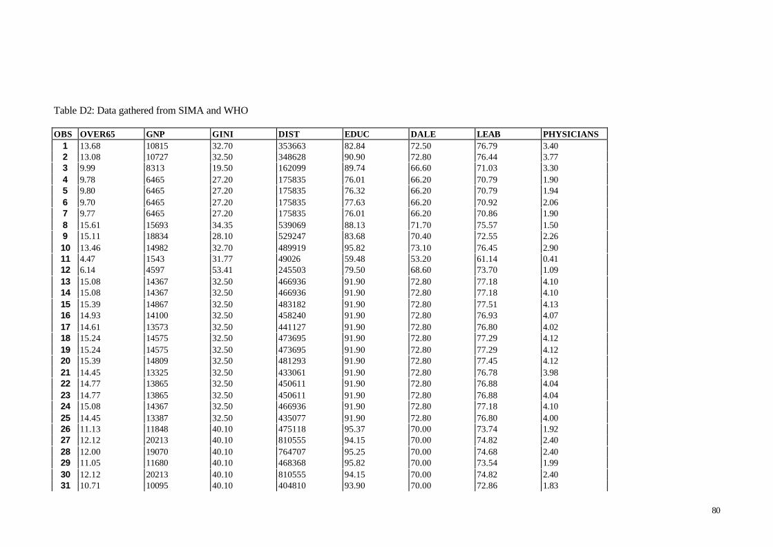
80
Table D2: Data gathered from SIMA and WHO
OBS OVER65 GNP GINI DIST EDUC DALE LEAB PHYSICIANS1 13.68 10815 32.70 353663 82.84 72.50 76.79 3.402 13.08 10727 32.50 348628 90.90 72.80 76.44 3.773 9.99 8313 19.50 162099 89.74 66.60 71.03 3.304 9.78 6465 27.20 175835 76.01 66.20 70.79 1.905 9.80 6465 27.20 175835 76.32 66.20 70.79 1.946 9.70 6465 27.20 175835 77.63 66.20 70.92 2.067 9.77 6465 27.20 175835 76.01 66.20 70.86 1.908 15.61 15693 34.35 539069 88.13 71.70 75.57 1.509 15.11 18834 28.10 529247 83.68 70.40 72.55 2.2610 13.46 14982 32.70 489919 95.82 73.10 76.45 2.9011 4.47 1543 31.77 49026 59.48 53.20 61.14 0.4112 6.14 4597 53.41 245503 79.50 68.60 73.70 1.0913 15.08 14367 32.50 466936 91.90 72.80 77.18 4.1014 15.08 14367 32.50 466936 91.90 72.80 77.18 4.1015 15.39 14867 32.50 483182 91.90 72.80 77.51 4.1316 14.93 14100 32.50 458240 91.90 72.80 76.93 4.0717 14.61 13573 32.50 441127 91.90 72.80 76.80 4.0218 15.24 14575 32.50 473695 91.90 72.80 77.29 4.1219 15.24 14575 32.50 473695 91.90 72.80 77.29 4.1220 15.39 14809 32.50 481293 91.90 72.80 77.45 4.1221 14.45 13325 32.50 433061 91.90 72.80 76.78 3.9822 14.77 13865 32.50 450611 91.90 72.80 76.88 4.0423 14.77 13865 32.50 450611 91.90 72.80 76.88 4.0424 15.08 14367 32.50 466936 91.90 72.80 77.18 4.1025 14.45 13387 32.50 435077 91.90 72.80 76.80 4.0026 11.13 11848 40.10 475118 95.37 70.00 73.74 1.9227 12.12 20213 40.10 810555 94.15 70.00 74.82 2.4028 12.00 19070 40.10 764707 95.25 70.00 74.68 2.4029 11.05 11680 40.10 468368 95.82 70.00 73.54 1.9930 12.12 20213 40.10 810555 94.15 70.00 74.82 2.4031 10.71 10095 40.10 404810 93.90 70.00 72.86 1.83
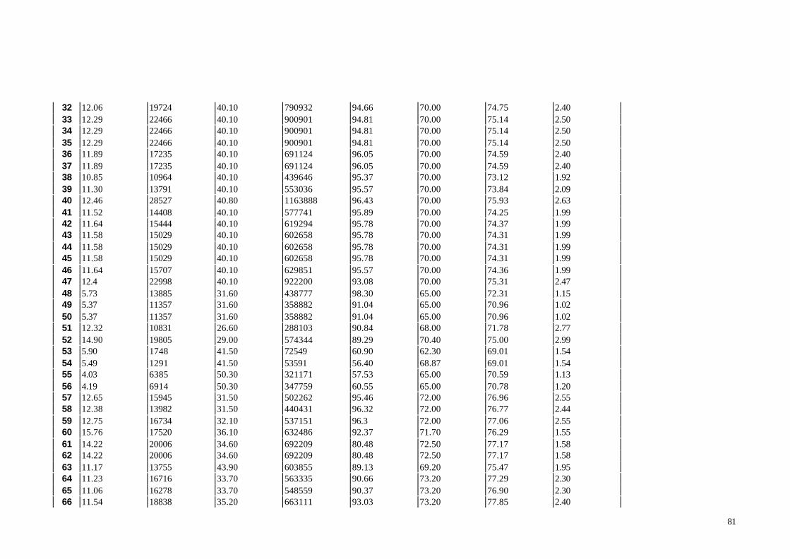
81
32 12.06 19724 40.10 790932 94.66 70.00 74.75 2.4033 12.29 22466 40.10 900901 94.81 70.00 75.14 2.5034 12.29 22466 40.10 900901 94.81 70.00 75.14 2.5035 12.29 22466 40.10 900901 94.81 70.00 75.14 2.5036 11.89 17235 40.10 691124 96.05 70.00 74.59 2.4037 11.89 17235 40.10 691124 96.05 70.00 74.59 2.4038 10.85 10964 40.10 439646 95.37 70.00 73.12 1.9239 11.30 13791 40.10 553036 95.57 70.00 73.84 2.0940 12.46 28527 40.80 1163888 96.43 70.00 75.93 2.6341 11.52 14408 40.10 577741 95.89 70.00 74.25 1.9942 11.64 15444 40.10 619294 95.78 70.00 74.37 1.9943 11.58 15029 40.10 602658 95.78 70.00 74.31 1.9944 11.58 15029 40.10 602658 95.78 70.00 74.31 1.9945 11.58 15029 40.10 602658 95.78 70.00 74.31 1.9946 11.64 15707 40.10 629851 95.57 70.00 74.36 1.9947 12.4 22998 40.10 922200 93.08 70.00 75.31 2.4748 5.73 13885 31.60 438777 98.30 65.00 72.31 1.1549 5.37 11357 31.60 358882 91.04 65.00 70.96 1.0250 5.37 11357 31.60 358882 91.04 65.00 70.96 1.0251 12.32 10831 26.60 288103 90.84 68.00 71.78 2.7752 14.90 19805 29.00 574344 89.29 70.40 75.00 2.9953 5.90 1748 41.50 72549 60.90 62.30 69.01 1.5454 5.49 1291 41.50 53591 56.40 68.87 69.01 1.5455 4.03 6385 50.30 321171 57.53 65.00 70.59 1.1356 4.19 6914 50.30 347759 60.55 65.00 70.78 1.2057 12.65 15945 31.50 502262 95.46 72.00 76.96 2.5558 12.38 13982 31.50 440431 96.32 72.00 76.77 2.4459 12.75 16734 32.10 537151 96.3 72.00 77.06 2.5560 15.76 17520 36.10 632486 92.37 71.70 76.29 1.5561 14.22 20006 34.60 692209 80.48 72.50 77.17 1.5862 14.22 20006 34.60 692209 80.48 72.50 77.17 1.5863 11.17 13755 43.90 603855 89.13 69.20 75.47 1.9564 11.23 16716 33.70 563335 90.66 73.20 77.29 2.3065 11.06 16278 33.70 548559 90.37 73.20 76.90 2.3066 11.54 18838 35.20 663111 93.03 73.20 77.85 2.40
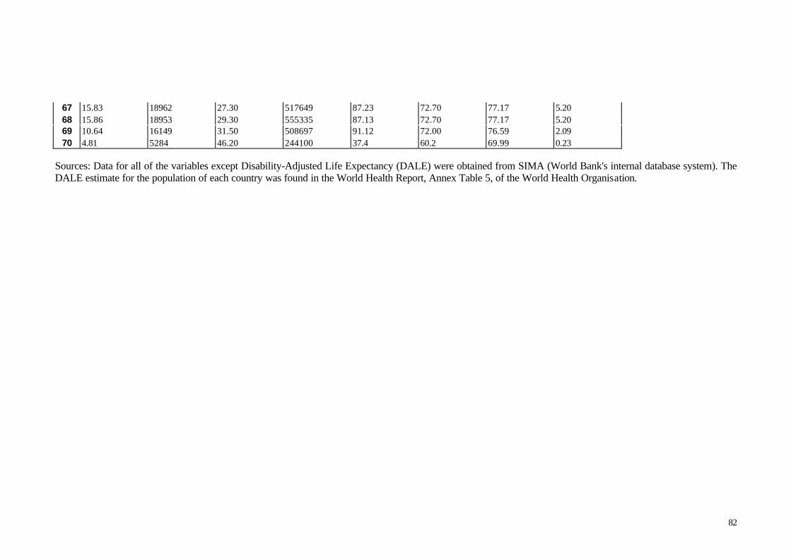
82
67 15.83 18962 27.30 517649 87.23 72.70 77.17 5.2068 15.86 18953 29.30 555335 87.13 72.70 77.17 5.2069 10.64 16149 31.50 508697 91.12 72.00 76.59 2.0970 4.81 5284 46.20 244100 37.4 60.2 69.99 0.23
Sources: Data for all of the variables except Disability-Adjusted Life Expectancy (DALE) were obtained from SIMA (World Bank's internal database system). TheDALE estimate for the population of each country was found in the World Health Report, Annex Table 5, of the World Health Organisation.
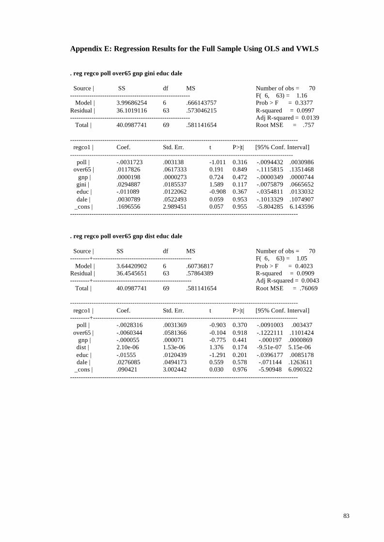
83
Appendix E: Regression Results for the Full Sample Using OLS and VWLS
. reg regco poll over65 gnp gini educ dale
Source | SS df MS Number of obs = 70-------------------------------------------------------- F( 6, 63) = 1.16 Model | 3.99686254 6 .666143757 Prob > F = 0.3377Residual | 36.1019116 63 .573046215 R-squared = 0.0997-------------------------------------------------------- Adj R-squared = 0.0139 Total | 40.0987741 69 .581141654 Root MSE = .757
---------------------------------------------------------------------------------------------------------- regco1 | Coef. Std. Err. t P>|t| [95% Conf. Interval]-------------------------------------------------------------------------------------------------------- poll | -.0031723 .003138 -1.011 0.316 -.0094432 .0030986 over65 | .0117826 .0617333 0.191 0.849 -.1115815 .1351468 gnp | .0000198 .0000273 0.724 0.472 -.0000349 .0000744 gini | .0294887 .0185537 1.589 0.117 -.0075879 .0665652 educ | -.011089 .0122062 -0.908 0.367 -.0354811 .0133032 dale | .0030789 .0522493 0.059 0.953 -.1013329 .1074907 _cons | .1696556 2.989451 0.057 0.955 -5.804285 6.143596----------------------------------------------------------------------------------------------------------
. reg regco poll over65 gnp dist educ dale
Source | SS df MS Number of obs = 70---------+---------------------------------------------- F( 6, 63) = 1.05 Model | 3.64420902 6 .60736817 Prob > F = 0.4023Residual | 36.4545651 63 .57864389 R-squared = 0.0909---------+---------------------------------------------- Adj R-squared = 0.0043 Total | 40.0987741 69 .581141654 Root MSE = .76069
---------------------------------------------------------------------------------------------------------- regco1 | Coef. Std. Err. t P>|t| [95% Conf. Interval]---------+----------------------------------------------------------------------------------------------- poll | -.0028316 .0031369 -0.903 0.370 -.0091003 .003437 over65 | -.0060344 .0581366 -0.104 0.918 -.1222111 .1101424 gnp | -.000055 .000071 -0.775 0.441 -.000197 .0000869 dist | 2.10e-06 1.53e-06 1.376 0.174 -9.51e-07 5.15e-06 educ | -.01555 .0120439 -1.291 0.201 -.0396177 .0085178 dale | .0276085 .0494173 0.559 0.578 -.071144 .1263611 _cons | .090421 3.002442 0.030 0.976 -5.90948 6.090322----------------------------------------------------------------------------------------------------------
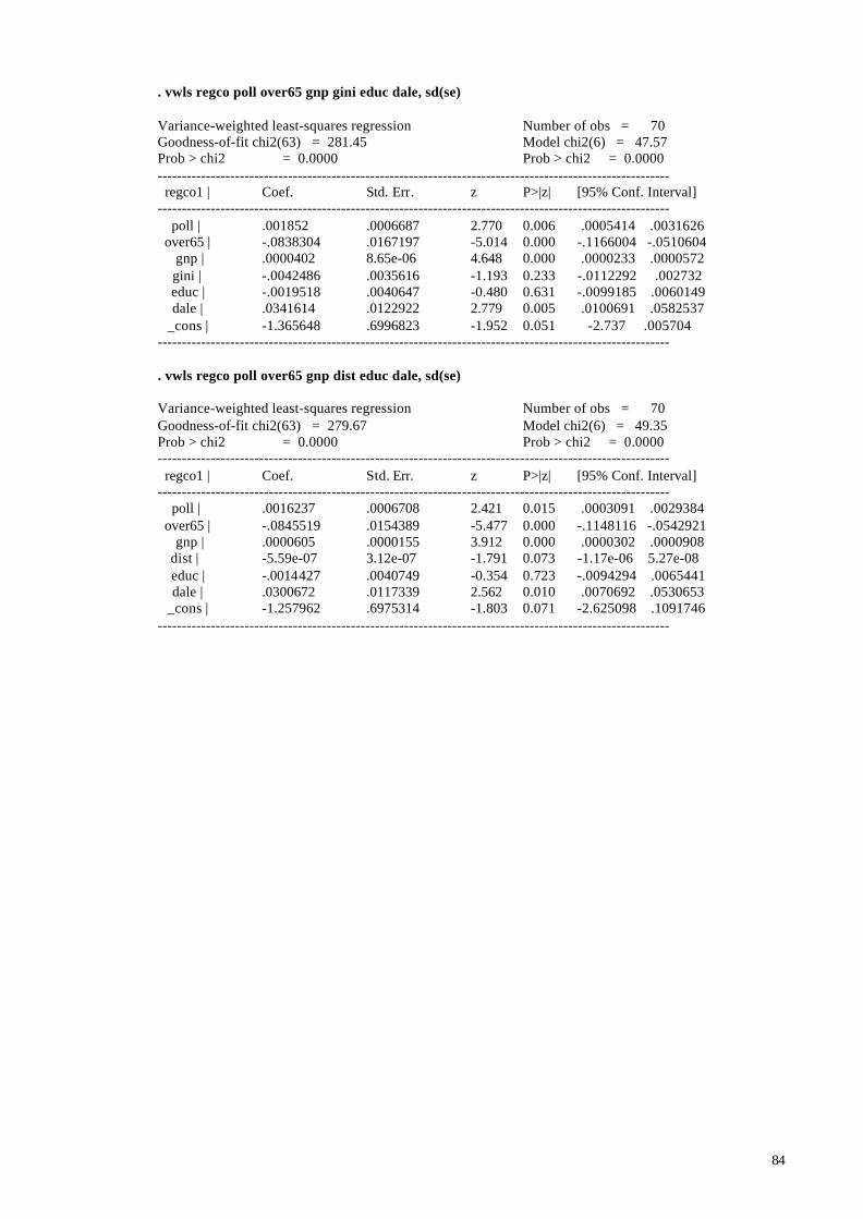
84
. vwls regco poll over65 gnp gini educ dale, sd(se)
Variance-weighted least-squares regression Number of obs = 70Goodness-of-fit chi2(63) = 281.45 Model chi2(6) = 47.57Prob > chi2 = 0.0000 Prob > chi2 = 0.0000---------------------------------------------------------------------------------------------------------- regco1 | Coef. Std. Err. z P>|z| [95% Conf. Interval]---------------------------------------------------------------------------------------------------------- poll | .001852 .0006687 2.770 0.006 .0005414 .0031626 over65 | -.0838304 .0167197 -5.014 0.000 -.1166004 -.0510604 gnp | .0000402 8.65e-06 4.648 0.000 .0000233 .0000572 gini | -.0042486 .0035616 -1.193 0.233 -.0112292 .002732 educ | -.0019518 .0040647 -0.480 0.631 -.0099185 .0060149 dale | .0341614 .0122922 2.779 0.005 .0100691 .0582537 _cons | -1.365648 .6996823 -1.952 0.051 -2.737 .005704----------------------------------------------------------------------------------------------------------
. vwls regco poll over65 gnp dist educ dale, sd(se)
Variance-weighted least-squares regression Number of obs = 70Goodness-of-fit chi2(63) = 279.67 Model chi2(6) = 49.35Prob > chi2 = 0.0000 Prob > chi2 = 0.0000---------------------------------------------------------------------------------------------------------- regco1 | Coef. Std. Err. z P>|z| [95% Conf. Interval]---------------------------------------------------------------------------------------------------------- poll | .0016237 .0006708 2.421 0.015 .0003091 .0029384 over65 | -.0845519 .0154389 -5.477 0.000 -.1148116 -.0542921 gnp | .0000605 .0000155 3.912 0.000 .0000302 .0000908 dist | -5.59e-07 3.12e-07 -1.791 0.073 -1.17e-06 5.27e-08 educ | -.0014427 .0040749 -0.354 0.723 -.0094294 .0065441 dale | .0300672 .0117339 2.562 0.010 .0070692 .0530653 _cons | -1.257962 .6975314 -1.803 0.071 -2.625098 .1091746----------------------------------------------------------------------------------------------------------
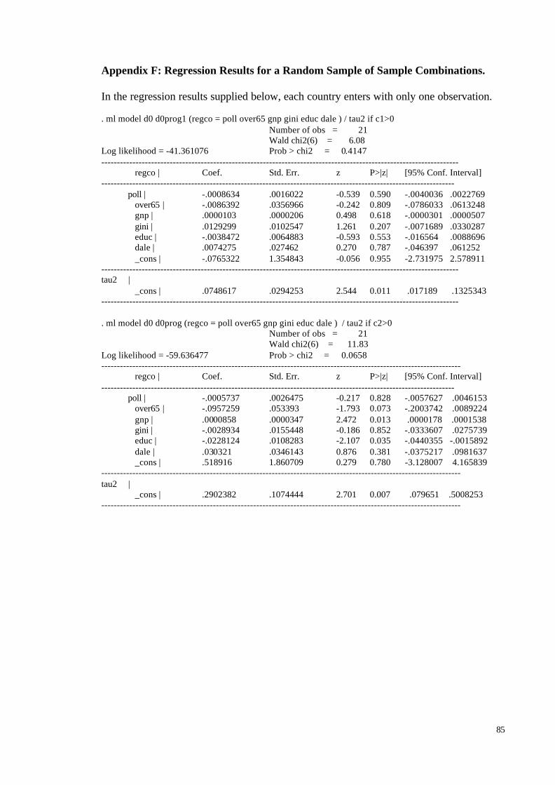
85
Appendix F: Regression Results for a Random Sample of Sample Combinations.
In the regression results supplied below, each country enters with only one observation.
. ml model d0 d0prog1 (regco = poll over65 gnp gini educ dale ) / tau2 if c1>0Number of obs = 21
Wald chi2(6) = 6.08Log likelihood = -41.361076 Prob > chi2 = 0.4147------------------------------------------------------------------------------------------------------------------- regco | Coef. Std. Err. z P>|z| [95% Conf. Interval]------------------------------------------------------------------------------------------------------------------
poll | -.0008634 .0016022 -0.539 0.590 -.0040036 .0022769 over65 | -.0086392 .0356966 -0.242 0.809 -.0786033 .0613248 gnp | .0000103 .0000206 0.498 0.618 -.0000301 .0000507 gini | .0129299 .0102547 1.261 0.207 -.0071689 .0330287 educ | -.0038472 .0064883 -0.593 0.553 -.016564 .0088696 dale | .0074275 .027462 0.270 0.787 -.046397 .061252 _cons | -.0765322 1.354843 -0.056 0.955 -2.731975 2.578911-------------------------------------------------------------------------------------------------------------------tau2 | _cons | .0748617 .0294253 2.544 0.011 .017189 .1325343-------------------------------------------------------------------------------------------------------------------
. ml model d0 d0prog (regco = poll over65 gnp gini educ dale ) / tau2 if c2>0 Number of obs = 21 Wald chi2(6) = 11.83Log likelihood = -59.636477 Prob > chi2 = 0.0658-------------------------------------------------------------------------------------------------------------------- regco | Coef. Std. Err. z P>|z| [95% Conf. Interval]------------------------------------------------------------------------------------------------------------------
poll | -.0005737 .0026475 -0.217 0.828 -.0057627 .0046153 over65 | -.0957259 .053393 -1.793 0.073 -.2003742 .0089224 gnp | .0000858 .0000347 2.472 0.013 .0000178 .0001538 gini | -.0028934 .0155448 -0.186 0.852 -.0333607 .0275739 educ | -.0228124 .0108283 -2.107 0.035 -.0440355 -.0015892 dale | .030321 .0346143 0.876 0.381 -.0375217 .0981637 _cons | .518916 1.860709 0.279 0.780 -3.128007 4.165839--------------------------------------------------------------------------------------------------------------------tau2 | _cons | .2902382 .1074444 2.701 0.007 .079651 .5008253--------------------------------------------------------------------------------------------------------------------

86
. ml model d0 d0prog3 (regco = poll over65 gnp gini educ dale ) / tau2 if c3> 0Number of obs = 21
Wald chi2(6) = 12.81Log likelihood = -46.552821 Prob > chi2 = 0.0462------------------------------------------------------------------------------------------------------------------- regco | Coef. Std. Err. z P>|z| [95% Conf. Interval]------------------------------------------------------------------------------------------------------------------
poll | -.0004785 .0013978 -0.342 0.732 -.0032181 .0022611 over65 | -.0058429 .0380754 -0.153 0.878 -.0804693 .0687835 gnp | 8.93e-06 .0000215 0.416 0.678 -.0000332 .000051 gini | .0117473 .0099307 1.183 0.237 -.0077166 .0312112 educ | -.0164378 .0070205 -2.341 0.019 -.0301978 -.0026778 dale | .0274064 .027457 0.998 0.318 -.0264083 .0812211 _cons | -.5030326 1.31468 -0.383 0.702 -3.079759 2.073694------------------------------------------------------------------------------------------------------------------tau2 | _cons | .0669139 .0361628 1.850 0.064 -.0039638 .1377916-------------------------------------------------------------------------------------------------------------------
. ml model d0 d0prog4 (regco = poll over65 gnp gini educ dale ) / tau2 if c4>0Number of obs = 21
Wald chi2(6) = 12.82Log likelihood = -56.603155 Prob > chi2 = 0.0460------------------------------------------------------------------------------------------------------------------- regco | Coef. Std. Err. z P>|z| [95% Conf. Interval]------------------------------------------------------------------------------------------------------------------
poll | .0026665 .002568 1.038 0.299 -.0023666 .0076996 over65 | .0534209 .047811 1.117 0.264 -.0402869 .1471288 gnp | .000069 .000031 2.222 0.026 8.15e-06 .0001298 gini | .022429 .0140201 1.600 0.110 -.0050498 .0499079 educ | -.0131625 .0086045 -1.530 0.126 -.0300271 .0037021 dale | -.0188534 .0313242 -0.602 0.547 -.0802477 .0425409 _cons | .6598235 1.636398 0.403 0.687 -2.547458 3.867105------------------------------------------------------------------------------------------------------------------tau2 | _cons | .2100956 .0834808 2.517 0.012 .0464763 .373715-------------------------------------------------------------------------------------------------------------------
. ml model d0 d0prog5 (regco = poll over65 gnp gini educ dale ) / tau2 if c5> 0Number of obs = 21
Wald chi2(6) = 20.96Log likelihood = -39.845363 Prob > chi2 = 0.0019------------------------------------------------------------------------------------------------------------------- regco | Coef. Std. Err. z P>|z| [95% Conf. Interval]------------------------------------------------------------------------------------------------------------------ poll | .0006733 .0014577 0.462 0.644 -.0021837 .0035302 over65 | -.1097985 .0293858 -3.736 0.000 -.1673936 -.0522033 gnp | .0000457 .0000188 2.433 0.015 8.89e-06 .0000826 gini | -.005942 .0081729 -0.727 0.467 -.0219607 .0100767 educ | -.0086456 .0061046 -1.416 0.157 -.0206103 .0033191 dale | .0405547 .0228899 1.772 0.076 -.0043087 .0854181 _cons | -.8398555 1.200993 -0.699 0.484 -3.193758 1.514047-------------------------------------------------------------------------------------------------------------------tau2 | _cons | .0551182 .0249164 2.212 0.027 .0062829 .1039535-------------------------------------------------------------------------------------------------------------------

87
. ml model d0 d0prog6 (regco = poll over65 gnp gini educ dale ) / tau2 if c6>0Number of obs = 21
Wald chi2(6) = 10.36Log likelihood = -60.052485 Prob > chi2 = 0.1105------------------------------------------------------------------------------------------------------------------- regco | Coef. Std. Err. z P>|z| [95% Conf. Interval]-------------------------------------------------------------------------------------------------------------------
poll | -.0011176 .002853 -0.392 0.695 -.0067094 .0044742 over65 | .0157608 .0593338 0.266 0.791 -.1005314 .1320529 gnp | .0000434 .0000409 1.062 0.288 -.0000367 .0001236 gini | .020833 .0160285 1.300 0.194 -.0105823 .0522484 educ | -.0217648 .0107806 -2.019 0.043 -.0428944 -.0006352 dale | .0076838 .0362123 0.212 0.832 -.063291 .0786586 _cons | .5178108 1.89681 0.273 0.785 -3.199869 4.235491-------------------------------------------------------------------------------------------------------------------tau2 | _cons | .3100155 .112988 2.744 0.006 .0885632 .5314679-------------------------------------------------------------------------------------------------------------------
. ml model d0 d0prog7 (regco = poll over65 gnp gini educ dale ) / tau2 if c7>0Number of obs = 21
Wald chi2(6) = 11.10Log likelihood = -50.665526 Prob > chi2 = 0.0852------------------------------------------------------------------------------------------------------------------- regco | Coef. Std. Err. z P>|z| [95% Conf. Interval]-------------------------------------------------------------------------------------------------------------------
poll | -.0008796 .0017237 -0.510 0.610 -.0042581 .0024988 over65 | -.020491 .0450024 -0.455 0.649 -.1086942 .0677121 gnp | .00004 .0000242 1.653 0.098 -7.43e-06 .0000874 gini | .0211933 .0125281 1.692 0.091 -.0033613 .0457478 educ | -.0060512 .0082835 -0.731 0.465 -.0222866 .0101843 dale | -.0073191 .0344719 -0.212 0.832 -.0748827 .0602445 _cons | .6446868 1.638074 0.394 0.694 -2.565879 3.855253-------------------------------------------------------------------------------------------------------------------tau2 | _cons | .1220844 .0483076 2.527 0.011 .0274033 .2167655-------------------------------------------------------------------------------------------------------------------
. ml model d0 d0prog8 (regco = poll over65 gnp gini educ dale ) / tau2 if c8>0 Number of obs = 21 Wald chi2(6) = 11.56Log likelihood = -57.789363 Prob > chi2 = 0.0724------------------------------------------------------------------------------------------------------------------- regco | Coef. Std. Err. z P>|z| [95% Conf. Interval]-------------------------------------------------------------------------------------------------------------------
poll | .0021584 .002653 0.814 0.416 -.0030414 .0073582 over65 | -.0557361 .0490866 -1.135 0.256 -.1519441 .0404719 gnp | .000095 .0000329 2.886 0.004 .0000305 .0001596 gini | .0022487 .0143583 0.157 0.876 -.025893 .0303903 educ | -.0144162 .0099787 -1.445 0.149 -.033974 .0051417 dale | .0154026 .03134 0.491 0.623 -.0460227 .0768278 _cons | -.0106618 1.692653 -0.006 0.995 -3.3282 3.306876-------------------------------------------------------------------------------------------------------------------tau2 | _cons | .2323947 .0916842 2.535 0.011 .0526969 .4120925-------------------------------------------------------------------------------------------------------------------

88
. ml model d0 d0prog9 (regco = poll over65 gnp gini educ dale ) / tau2 if c9>0Number of obs = 21
Wald chi2(6) = 20.60Log likelihood = -36.620218 Prob > chi2 = 0.0022------------------------------------------------------------------------------------------------------------------- regco | Coef. Std. Err. z P>|z| [95% Conf. Interval]-------------------------------------------------------------------------------------------------------------------
poll | .0005383 .0011383 0.473 0.636 -.0016928 .0027694 over65 | -.0262215 .0278982 -0.940 0.347 -.0809011 .028458 gnp | .000017 .0000148 1.153 0.249 -.0000119 .000046 gini | .0044916 .0068194 0.659 0.510 -.0088743 .0178574 educ | -.0163131 .0052966 -3.080 0.002 -.0266943 -.0059319 dale | .0362147 .0190977 1.896 0.058 -.0012162 .0736455 _cons | -.8936275 .9963862 -0.897 0.370 -2.846509 1.059254-------------------------------------------------------------------------------------------------------------------tau2 | _cons | .0270157 .0143073 1.888 0.059 -.0010261 .0550575-------------------------------------------------------------------------------------------------------------------
. ml model d0 d0prog10 (regco = poll over65 gnp gini educ dale ) / tau2 if c10>0Number of obs = 21
Wald chi2(6) = 11.38Log likelihood = -59.331796 Prob > chi2 = 0.0772------------------------------------------------------------------------------------------------------------------- regco | Coef. Std. Err. z P>|z| [95% Conf. Interval]-------------------------------------------------------------------------------------------------------------------
poll | -.0004563 .0025717 -0.177 0.859 -.0054968 .0045842 over65 | .0150591 .0538812 0.279 0.780 -.0905461 .1206643 gnp | .0000571 .0000308 1.858 0.063 -3.13e-06 .0001174 gini | .0164117 .0159063 1.032 0.302 -.0147641 .0475875 educ | -.0202872 .0102959 -1.970 0.049 -.0404668 -.0001075 dale | -.0036402 .0345555 -0.105 0.916 -.0713676 .0640873 _cons | 1.174953 1.795952 0.654 0.513 -2.345049 4.694956-------------------------------------------------------------------------------------------------------------------tau2 | _cons | .264388 .1024882 2.580 0.010 .0635148 .4652612-------------------------------------------------------------------------------------------------------------------
. ml model d0 d0prog11 (regco = poll over65 gnp gini educ dale ) / tau2 if c11>0Number of obs = 21
Wald chi2(6) = 14.21Log likelihood = -46.567254 Prob > chi2 = 0.0273------------------------------------------------------------------------------------------------------------------- regco | Coef. Std. Err. z P>|z| [95% Conf. Interval]-------------------------------------------------------------------------------------------------------------------
poll | -.0005675 .001445 -0.393 0.695 -.0033995 .0022646 over65 | -.0946786 .034787 -2.722 0.006 -.16286 -.0264973 gnp | .0000355 .0000225 1.574 0.116 -8.71e-06 .0000797 gini | .0008488 .0098769 0.086 0.932 -.0185097 .0202072 educ | -.0096141 .0071078 -1.353 0.176 -.0235452 .004317 dale | .038468 .0273919 1.404 0.160 -.0152191 .0921552 _cons | -.7223563 1.318953 -0.548 0.584 -3.307457 1.862745-------------------------------------------------------------------------------------------------------------------tau2 | _cons | .0714972 .0340504 2.100 0.036 .0047597 .1382347-------------------------------------------------------------------------------------------------------------------

89
. ml model d0 d0prog12 (regco = poll over65 gnp gini educ dale ) / tau2 if c12>0Number of obs = 21
Wald chi2(6) = 13.37Log likelihood = -60.762544 Prob > chi2 = 0.0376------------------------------------------------------------------------------------------------------------------- regco | Coef. Std. Err. z P>|z| [95% Conf. Interval]-------------------------------------------------------------------------------------------------------------------
poll | .0023236 .002649 0.877 0.380 -.0028682 .0075155 over65 | .0138613 .0516725 0.268 0.789 -.0874149 .1151375 gnp | .0000739 .000036 2.056 0.040 3.45e-06 .0001444 gini | .0103033 .0142352 0.724 0.469 -.0175972 .0382038 educ | -.023356 .0098721 -2.366 0.018 -.0427051 -.004007 dale | .0107396 .0310045 0.346 0.729 -.0500281 .0715073 _cons | .1546618 1.654462 0.093 0.926 -3.088025 3.397349-------------------------------------------------------------------------------------------------------------------tau2 | _cons | .2184805 .0934211 2.339 0.019 .0353786 .4015825-------------------------------------------------------------------------------------------------------------------
. ml model d0 d0prog13 (regco = poll over65 gnp gini educ dale ) / tau2 if c13>0Number of obs = 21
Wald chi2(6) = 6.75Log likelihood = -53.687934 Prob > chi2 = 0.3445------------------------------------------------------------------------------------------------------------------- regco | Coef. Std. Err. z P>|z| [95% Conf. Interval]-------------------------------------------------------------------------------------------------------------------
poll | -.0008195 .0018503 -0.443 0.658 -.004446 .002807 over65 | -.0352514 .0395734 -0.891 0.373 -.1128139 .042311 gnp | .0000246 .0000248 0.993 0.321 -.000024 .0000733 gini | .0117938 .0116333 1.014 0.311 -.011007 .0345947 educ | -.0045706 .0071821 -0.636 0.525 -.0186472 .009506 dale | .0036871 .0319272 0.115 0.908 -.058889 .0662632 _cons | .3479319 1.575462 0.221 0.825 -2.739917 3.435781-------------------------------------------------------------------------------------------------------------------tau2 | _cons | .1082984 .0518228 2.090 0.037 .0067275 .2098693-------------------------------------------------------------------------------------------------------------------
. ml model d0 d0prog14 (regco = poll over65 gnp gini educ dale ) / tau2 if c14>0Number of obs = 21
Wald chi2(6) = 10.32Log likelihood = -58.404488 Prob > chi2 = 0.1119------------------------------------------------------------------------------------------------------------------- regco | Coef. Std. Err. z P>|z| [95% Conf. Interval]-------------------------------------------------------------------------------------------------------------------
poll | .0002928 .0027661 0.106 0.916 -.0051286 .0057142 over65 | -.0668596 .0534701 -1.250 0.211 -.1716591 .03794 gnp | .000087 .000039 2.228 0.026 .0000105 .0001635 gini | .0055993 .0147901 0.379 0.705 -.0233886 .0345873 educ | -.018301 .0100758 -1.816 0.069 -.0380492 .0014471 dale | .0208245 .0333586 0.624 0.532 -.0445571 .0862061 _cons | .2107019 1.785615 0.118 0.906 -3.289038 3.710442-------------------------------------------------------------------------------------------------------------------tau2 | _cons | .267619 .1003434 2.667 0.008 .0709495 .4642885-------------------------------------------------------------------------------------------------------------------
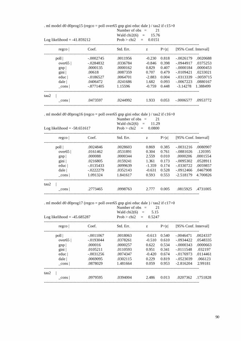
90
. ml model d0 d0prog15 (regco = poll over65 gnp gini educ dale ) / tau2 if c15>0Number of obs = 21
Wald chi2(6) = 15.76Log likelihood = -41.859212 Prob > chi2 = 0.0151------------------------------------------------------------------------------------------------------------------- regco | Coef. Std. Err. z P>|z| [95% Conf. Interval]-------------------------------------------------------------------------------------------------------------------
poll | -.0002745 .0011956 -0.230 0.818 -.0026179 .0020688 over65 | -.0284832 .0336784 -0.846 0.398 -.0944917 .0375253 gnp | .0000135 .0000162 0.829 0.407 -.0000184 .0000453 gini | .00618 .0087359 0.707 0.479 -.0109421 .0233021 educ | -.0186527 .0064701 -2.883 0.004 -.0313339 -.0059715 dale | .0406472 .0241686 1.682 0.093 -.0067223 .0880167 _cons | -.8771405 1.15596 -0.759 0.448 -3.14278 1.388499-------------------------------------------------------------------------------------------------------------------tau2 | _cons | .0473597 .0244992 1.933 0.053 -.0006577 .0953772-------------------------------------------------------------------------------------------------------------------
. ml model d0 d0prog16 (regco = poll over65 gnp gini educ dale ) / tau2 if c16>0Number of obs = 21
Wald chi2(6) = 11.29Log likelihood = -58.651617 Prob > chi2 = 0.0800------------------------------------------------------------------------------------------------------------------- regco | Coef. Std. Err. z P>|z| [95% Conf. Interval]-------------------------------------------------------------------------------------------------------------------
poll | .0024846 .0028603 0.869 0.385 -.0031216 .0080907 over65 | .0161462 .0531891 0.304 0.761 -.0881026 .120395 gnp | .000088 .0000344 2.559 0.010 .0000206 .0001554 gini | .0216805 .0159241 1.361 0.173 -.0095302 .0528911 educ | -.0135433 .0099639 -1.359 0.174 -.0330722 .0059857 dale | -.0222279 .0352143 -0.631 0.528 -.0912466 .0467908 _cons | 1.091324 1.841617 0.593 0.553 -2.518179 4.700826-------------------------------------------------------------------------------------------------------------------tau2 | _cons | .2773465 .0998763 2.777 0.005 .0815925 .4731005-------------------------------------------------------------------------------------------------------------------
. ml model d0 d0prog17 (regco = poll over65 gnp gini educ dale ) / tau2 if c17>0Number of obs = 21
Wald chi2(6) = 5.15Log likelihood = -45.685287 Prob > chi2 = 0.5247------------------------------------------------------------------------------------------------------------------- regco | Coef. Std. Err. z P>|z| [95% Conf. Interval]-------------------------------------------------------------------------------------------------------------------
poll | -.0011067 .0018063 -0.613 0.540 -.0046471 .0024337 over65 | -.0193044 .0378261 -0.510 0.610 -.0934422 .0548335 gnp | .000016 .0000257 0.622 0.534 -.0000343 .0000663 gini | .0105211 .0110593 0.951 0.341 -.0111548 .032197 educ | -.0031256 .0074347 -0.420 0.674 -.0176973 .0114461 dale | .0069095 .0302115 0.229 0.819 -.0523039 .066123 _cons | .0878029 1.481664 0.059 0.953 -2.816204 2.99181-------------------------------------------------------------------------------------------------------------------tau2 | _cons | .0979595 .0394004 2.486 0.013 .0207362 .1751828-------------------------------------------------------------------------------------------------------------------
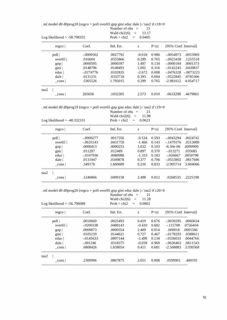
91
. ml model d0 d0prog18 (regco = poll over65 gnp gini educ dale ) / tau2 if c18>0Number of obs = 21
Wald chi2(6) = 13.17Log likelihood = -58.798355 Prob > chi2 = 0.0405------------------------------------------------------------------------------------------------------------------- regco | Coef. Std. Err. z P>|z| [95% Conf. Interval]-------------------------------------------------------------------------------------------------------------------
poll | -.0000502 .0027792 -0.018 0.986 -.0054973 .0053969 over65 | .016604 .0555866 0.299 0.765 -.0923438 .1255518 gnp | .0000595 .0000397 1.497 0.134 -.0000184 .0001373 gini | .0148796 .0148493 1.002 0.316 -.0142245 .0439837 educ | -.0274776 .0102835 -2.672 0.008 -.0476328 -.0073223 dale | .0131231 .0333718 0.393 0.694 -.0522845 .0785306 _cons | .5365526 1.795015 0.299 0.765 -2.981612 4.054717-------------------------------------------------------------------------------------------------------------------tau2 | _cons | 265658 .1032305 2.573 0.010 .0633298 .4679861-------------------------------------------------------------------------------------------------------------------
. ml model d0 d0prog19 (regco = poll over65 gnp gini educ dale ) / tau2 if c19>0Number of obs = 21
Wald chi2(6) = 11.98Log likelihood = -48.332331 Prob > chi2 = 0.0623------------------------------------------------------------------------------------------------------------------- regco | Coef. Std. Err. z P>|z| [95% Conf. Interval]-------------------------------------------------------------------------------------------------------------------
poll | -.0009277 .0017356 -0.534 0.593 -.0043294 .0024741 over65 | -.0633143 .0431759 -1.466 0.143 -.1479376 .0213089 gnp | .0000413 .0000253 1.632 0.103 -8.30e-06 .0000909 gini | .011207 .012489 0.897 0.370 -.013271 .035685 educ | -.0107936 .0080988 -1.333 0.183 -.026667 .0050798 dale | .0131947 .0349878 0.377 0.706 -.0553802 .0817696 _cons | .349176 1.660689 0.210 0.833 -2.905714 3.604066-------------------------------------------------------------------------------------------------------------------tau2 | _cons | .1246866 .0499158 2.498 0.012 .0268535 .2225198-------------------------------------------------------------------------------------------------------------------
. ml model d0 d0prog20 (regco = poll over65 gnp gini educ dale ) / tau2 if c20>0Number of obs = 21
Wald chi2(6) = 11.28Log likelihood = -56.706088 Prob > chi2 = 0.0802------------------------------------------------------------------------------------------------------------------- regco | Coef. Std. Err. z P>|z| [95% Conf. Interval]-------------------------------------------------------------------------------------------------------------------
poll | .0010669 .0025493 0.419 0.676 -.0039295 .0060634 over65 | -.0200338 .0488143 -0.410 0.682 -.115708 .0756404 gnp | .0000873 .0000354 2.469 0.014 .000018 .0001566 gini | .0105159 .0144621 0.727 0.467 -.0178293 .0388611 educ | -.0145633 .0097144 -1.499 0.134 -.0336033 .0044766 dale | -.001246 .0318375 -0.039 0.969 -.0636463 .0611543 _cons | .6808426 1.658054 0.411 0.681 -2.568883 3.930568-------------------------------------------------------------------------------------------------------------------tau2 | _cons | .2300906 .0867875 2.651 0.008 .0599901 .400191-------------------------------------------------------------------------------------------------------------------

92
. ml model d0 d0prog21 (regco = poll over65 gnp gini educ dale ) / tau2 if c21>0Number of obs = 21
Wald chi2(6) = 21.63Log likelihood = -41.592121 Prob > chi2 = 0.0014------------------------------------------------------------------------------------------------------------------- regco | Coef. Std. Err. z P>|z| [95% Conf. Interval]-------------------------------------------------------------------------------------------------------------------
poll | .0004138 .0013287 0.311 0.755 -.0021905 .0030181 over65 | -.0163723 .0310397 -0.527 0.598 -.077209 .0444644 gnp | 3.17e-06 .0000194 0.163 0.870 -.0000349 .0000413 gini | .000022 .007641 0.003 0.998 -.014954 .0149981 educ | -.0205853 .0056896 -3.618 0.000 -.0317367 -.009434 dale | .0500904 .0212421 2.358 0.018 .0084567 .091724 _cons | -1.282094 1.096724 -1.169 0.242 -3.431634 .8674454-------------------------------------------------------------------------------------------------------------------tau2 | _cons | .0396367 .021711 1.826 0.068 -.002916 .0821895-------------------------------------------------------------------------------------------------------------------
. ml model d0 d0prog22 (regco = poll over65 gnp gini educ dale ) / tau2 if c22>0Number of obs = 21
Wald chi2(6) = 11.09Log likelihood = -60.190957 Prob > chi2 = 0.0857------------------------------------------------------------------------------------------------------------------- regco | Coef. Std. Err. z P>|z| [95% Conf. Interval]-------------------------------------------------------------------------------------------------------------------
poll | -.0006364 .0025486 -0.250 0.803 -.0056315 .0043587 over65 | .0214666 .055022 0.390 0.696 -.0863746 .1293078 gnp | .0000544 .0000308 1.765 0.078 -6.02e-06 .0001148 gini | .0176825 .0163909 1.079 0.281 -.0144432 .0498081 educ | -.0197888 .0105649 -1.873 0.061 -.0404956 .000918 dale | -.0054879 .03559 -0.154 0.877 -.075243 .0642673 _cons | 1.204919 1.845444 0.653 0.514 -2.412084 4.821923-------------------------------------------------------------------------------------------------------------------tau2 | _cons | .27935 .1080409 2.586 0.010 .0675938 .4911062-------------------------------------------------------------------------------------------------------------------
. ml model d0 d0prog23 (regco = poll over65 gnp gini educ dale ) / tau2 if c23>0Number of obs = 21
Wald chi2(6) = 10.67Log likelihood = -49.11387 Prob > chi2 = 0.0992------------------------------------------------------------------------------------------------------------------- regco | Coef. Std. Err. z P>|z| [95% Conf. Interval]-------------------------------------------------------------------------------------------------------------------
poll | -.001356 .0015867 -0.855 0.393 -.0044658 .0017539 over65 | -.0680085 .0376535 -1.806 0.071 -.1418081 .005791 gnp | .0000292 .0000234 1.247 0.212 -.0000167 .0000751 gini | .0056402 .0118187 0.477 0.633 -.017524 .0288045 educ | -.0099035 .0077477 -1.278 0.201 -.0250888 .0052819 dale | .0248575 .0326064 0.762 0.446 -.0390498 .0887649 _cons | -.0674224 1.511432 -0.045 0.964 -3.029776 2.894931-------------------------------------------------------------------------------------------------------------------tau2 | _cons | .0993821 .0431607 2.303 0.021 .0147886 .1839756-------------------------------------------------------------------------------------------------------------------

93
. ml model d0 d0prog24 (regco = poll over65 gnp gini educ dale ) / tau2 if c24>0Number of obs = 21
Wald chi2(6) = 10.94Log likelihood = -56.772328 Prob > chi2 = 0.0904------------------------------------------------------------------------------------------------------------------- regco | Coef. Std. Err. z P>|z| [95% Conf. Interval]-------------------------------------------------------------------------------------------------------------------
poll | .0024793 .0026744 0.927 0.354 -.0027624 .007721 over65 | -.0315979 .0448144 -0.705 0.481 -.1194325 .0562366 gnp | .0000877 .0000348 2.519 0.012 .0000195 .000156 gini | .0041463 .014192 0.292 0.770 -.0236695 .0319621 educ | -.0195454 .0097068 -2.014 0.044 -.0385704 -.0005204 dale | .0130661 .0314044 0.416 0.677 -.0484854 .0746177 _cons | .2302503 1.662984 0.138 0.890 -3.029138 3.489638-------------------------------------------------------------------------------------------------------------------tau2 | _cons | .2231022 .0862486 2.587 0.010 .054058 .3921464-------------------------------------------------------------------------------------------------------------------
. ml model d0 d0pro (regco1 = poll over65 gnp dist educ dale ) / tau2 if c1>0Number of obs = 21
Wald chi2(6) = 4.81Log likelihood = -60.497596 Prob > chi2 = 0.5684------------------------------------------------------------------------------------------------------------------- regco | Coef. Std. Err. z P>|z| [95% Conf. Interval]-------------------------------------------------------------------------------------------------------------------
poll | -.0005431 .0016626 -0.327 0.744 -.0038017 .0027155 over65 | -.0278231 .0316119 -0.880 0.379 -.0897813 .0341351 gnp | -9.20e-06 .0000369 -0.249 0.803 -.0000815 .0000631 dist | 6.32e-07 1.00e-06 0.631 0.528 -1.33e-06 2.60e-06 educ | -.0065429 .0060171 -1.087 0.277 -.0183361 .0052503 dale | .0235745 .023129 1.019 0.308 -.0217576 .0689066 _cons | -.3484194 1.341302 -0.260 0.795 -2.977324 2.280485-------------------------------------------------------------------------------------------------------------------tau2 | _cons | .0766539 .0310815 2.466 0.014 .0157353 .1375724-------------------------------------------------------------------------------------------------------------------
. ml model d0 d0pro2 (regco = poll over65 gnp dist educ dale ) / tau2 if c2>0 Number of obs = 21 Wald chi2(6) = 12.26Log likelihood = -78.018915 Prob > chi2 = 0.0565------------------------------------------------------------------------------------------------------------------- regco | Coef. Std. Err. z P>|z| [95% Conf. Interval]-------------------------------------------------------------------------------------------------------------------
poll | -.0006192 .0026217 -0.236 0.813 -.0057576 .0045192 over65 | -.1016589 .0494967 -2.054 0.040 -.1986706 -.0046472 gnp | .000117 .0000667 1.754 0.079 -.0000138 .0002478 dist | -8.32e-07 1.46e-06 -0.570 0.569 -3.69e-06 2.03e-06 educ | -.023113 .0100144 -2.308 0.021 -.0427408 -.0034852 dale | .0305877 .0306722 0.997 0.319 -.0295287 .090704 _cons | .453215 1.84617 0.245 0.806 -3.165212 4.071642-------------------------------------------------------------------------------------------------------------------tau2 | _cons | .2835818 .1062127 2.670 0.008 .0754087 .4917548-------------------------------------------------------------------------------------------------------------------

94
. ml model d0 d0pro3 (regco = poll over65 gnp dist educ dale ) / tau2 if c3>0 Number of obs = 21 Wald chi2(6) = 11.96Log likelihood = -65.572493 Prob > chi2 = 0.0630------------------------------------------------------------------------------------------------------------------- regco | Coef. Std. Err. z P>|z| [95% Conf. Interval]-------------------------------------------------------------------------------------------------------------------
poll | -.0000771 .0013923 -0.055 0.956 -.002806 .0026518 over65 | -.0204152 .0340243 -0.600 0.548 -.0871016 .0462713 gnp | -.0000154 .0000388 -0.398 0.691 -.0000914 .0000605 dist | 7.86e-07 9.00e-07 0.874 0.382 -9.77e-07 2.55e-06 educ | -.0190203 .0065926 -2.885 0.004 -.0319415 -.0060991 dale | .0418641 .0231024 1.812 0.070 -.0034159 .087144 _cons | -.7634688 1.296464 -0.589 0.556 -3.304491 1.777554-------------------------------------------------------------------------------------------------------------------tau2 | _cons | .0696536 .0378484 1.840 0.066 -.0045279 .1438352-------------------------------------------------------------------------------------------------------------------
. ml model d0 d0pro4 (regco = poll over65 gnp dist educ dale ) / tau2 if c4>0 Number of obs = 21 Wald chi2(6) = 11.37Log likelihood = -75.447562 Prob > chi2 = 0.0777------------------------------------------------------------------------------------------------------------------- regco | Coef. Std. Err. z P>|z| [95% Conf. Interval]-------------------------------------------------------------------------------------------------------------------
poll | .003088 .0027298 1.131 0.258 -.0022622 .0084382 over65 | .0354656 .0455506 0.779 0.436 -.053812 .1247432 gnp | .0000126 .0000576 0.219 0.827 -.0001003 .0001255 dist | 1.83e-06 1.48e-06 1.238 0.216 -1.07e-06 4.74e-06 educ | -.0166334 .0084025 -1.980 0.048 -.0331019 -.0001648 dale | -.0030375 .0288789 -0.105 0.916 -.059639 .0535641 _cons | .7467562 1.709996 0.437 0.662 -2.604775 4.098287-------------------------------------------------------------------------------------------------------------------tau2 | _cons | .2300362 .087502 2.629 0.009 .0585355 .4015369-------------------------------------------------------------------------------------------------------------------
. ml model d0 d0pro5 (regco = poll over65 gnp dist educ dale ) / tau2 if c5>0Number of obs = 21
Wald chi2(6) = 22.62Log likelihood = -58.125198 Prob > chi2 = 0.0009------------------------------------------------------------------------------------------------------------------- regco | Coef. Std. Err. z P>|z| [95% Conf. Interval]-------------------------------------------------------------------------------------------------------------------
poll | .0004273 .0014068 0.304 0.761 -.0023299 .0031845 over65 | -.1096787 .0256529 -4.275 0.000 -.1599574 -.0594 gnp | .0000739 .0000319 2.312 0.021 .0000113 .0001365 dist | -8.21e-07 7.08e-07 -1.159 0.247 -2.21e-06 5.67e-07 educ | -.0078769 .0056303 -1.399 0.162 -.018912 .0031583 dale | .0362322 .0191027 1.897 0.058 -.0012085 .0736729 _cons | -.8023469 1.1521 -0.696 0.486 -3.060421 1.455727-------------------------------------------------------------------------------------------------------------------tau2 | _cons | .0512909 .0240112 2.136 0.033 .0042299 .098352-------------------------------------------------------------------------------------------------------------------

95
. ml model d0 d0pro6 (regco = poll over65 gnp dist educ dale ) / tau2 if c6>0 Number of obs = 21 Wald chi2(6) = 9.76Log likelihood = -78.58854 Prob > chi2 = 0.1352------------------------------------------------------------------------------------------------------------------- regco | Coef. Std. Err. z P>|z| [95% Conf. Interval]-------------------------------------------------------------------------------------------------------------------
poll | -.0006427 .0029719 -0.216 0.829 -.0064675 .0051822 over65 | -.0011285 .056405 -0.020 0.984 -.1116803 .1094232 gnp | -.0000152 .0000677 -0.225 0.822 -.000148 .0001175 dist | 1.92e-06 1.69e-06 1.137 0.255 -1.39e-06 5.23e-06 educ | -.0246351 .0104321 -2.361 0.018 -.0450816 -.0041885 dale | .0214091 .0331944 0.645 0.519 -.0436507 .0864688 _cons | .6189596 1.941824 0.319 0.750 -3.186945 4.424864-------------------------------------------------------------------------------------------------------------------tau2 | _cons | .3241059 .1150498 2.817 0.005 .0986124 .5495994-------------------------------------------------------------------------------------------------------------------
. ml model d0 d0pro7 (regco = poll over65 gnp dist educ dale ) / tau2 if c7>0 Number of obs = 21 Wald chi2(6) = 10.55Log likelihood = -69.649745 Prob > chi2 = 0.1034------------------------------------------------------------------------------------------------------------------- regco | Coef. Std. Err. z P>|z| [95% Conf. Interval]-------------------------------------------------------------------------------------------------------------------
poll | -.0001605 .0017096 -0.094 0.925 -.0035112 .0031903 over65 | -.0413539 .0393238 -1.052 0.293 -.1184271 .0357193 gnp | -.000014 .0000462 -0.303 0.762 -.0001046 .0000766 dist | 1.67e-06 1.09e-06 1.533 0.125 -4.65e-07 3.81e-06 educ | -.0105373 .0074536 -1.414 0.157 -.0251461 .0040715 dale | .016358 .028497 0.574 0.566 -.0394951 .0722111 _cons | .2807918 1.609129 0.174 0.861 -2.873044 3.434627-------------------------------------------------------------------------------------------------------------------tau2 | _cons | .1247839 .0491282 2.540 0.011 .0284944 .2210734-------------------------------------------------------------------------------------------------------------------
. ml model d0 d0pro8 (regco = poll over65 gnp dist educ dale ) / tau2 if c8>0Number of obs = 21
Wald chi2(6) = 11.55Log likelihood = -76.281458 Prob > chi2 = 0.0729------------------------------------------------------------------------------------------------------------------- regco | Coef. Std. Err. z P>|z| [95% Conf. Interval]-------------------------------------------------------------------------------------------------------------------
poll | .0021756 .0026497 0.821 0.412 -.0030176 .0073688 over65 | -.0600763 .0457228 -1.314 0.189 -.1496913 .0295387 gnp | .0000973 .0000624 1.559 0.119 -.000025 .0002195 dist | -2.94e-08 1.39e-06 -0.021 0.983 -2.76e-06 2.70e-06 educ | -.0150989 .0093288 -1.619 0.106 -.0333829 .0031852 dale | .0179741 .0278018 0.647 0.518 -.0365164 .0724646 _cons | -.0228719 1.693375 -0.014 0.989 -3.341826 3.296083-------------------------------------------------------------------------------------------------------------------tau2 | _cons | .2315559 .0914157 2.533 0.011 .0523845 .4107273-------------------------------------------------------------------------------------------------------------------

96
. ml model d0 d0pro9 (regco = poll over65 gnp dist educ dale ) / tau2 if c9>0 Number of obs = 21 Wald chi2(6) = 20.25Log likelihood = -55.524752 Prob > chi2 = 0.0025------------------------------------------------------------------------------------------------------------------- regco | Coef. Std. Err. z P>|z| [95% Conf. Interval]-------------------------------------------------------------------------------------------------------------------
poll | .0006483 .0011288 0.574 0.566 -.0015641 .0028607 over65 | -.0373089 .0245416 -1.520 0.128 -.0854096 .0107918 gnp | .0000179 .0000273 0.656 0.512 -.0000355 .0000713 dist | 3.58e-08 5.97e-07 0.060 0.952 -1.13e-06 1.21e-06 educ | -.0171846 .0051096 -3.363 0.001 -.0271992 -.00717 dale | .0427803 .0162099 2.639 0.008 .0110094 .0745512 _cons | -1.026349 .9723321 -1.056 0.291 -2.932085 .8793869-------------------------------------------------------------------------------------------------------------------tau2 | _cons | .0267869 .01464 1.830 0.067 -.001907 .0554809-------------------------------------------------------------------------------------------------------------------
. ml model d0 d0pro10 (regco = poll over65 gnp dist educ dale ) / tau2 if c10>0Number of obs = 21
Wald chi2(6) = 10.30Log likelihood = -78.306758 Prob > chi2 = 0.1124------------------------------------------------------------------------------------------------------------------- regco | Coef. Std. Err. z P>|z| [95% Conf. Interval]-------------------------------------------------------------------------------------------------------------------
poll | -.0004811 .0026426 -0.182 0.856 -.0056605 .0046983 over65 | -.006102 .0500868 -0.122 0.903 -.1042704 .0920663 gnp | .000035 .0000664 0.527 0.598 -.0000951 .0001651 dist | 7.60e-07 1.50e-06 0.506 0.613 -2.18e-06 3.70e-06 educ | -.0238628 .0097586 -2.445 0.014 -.0429893 -.0047362 dale | .0115143 .0309565 0.372 0.710 -.0491594 .072188 _cons | 1.186873 1.840355 0.645 0.519 -2.420156 4.793902-------------------------------------------------------------------------------------------------------------------tau2 | _cons | .2785972 .106044 2.627 0.009 .0707547 .4864396-------------------------------------------------------------------------------------------------------------------
. ml model d0 d0pro11 (regco = poll over65 gnp dist educ dale ) / tau2 if c11>0 Number of obs = 21 Wald chi2(6) = 14.81Log likelihood = -65.109379 Prob > chi2 = 0.0218------------------------------------------------------------------------------------------------------------------- regco | Coef. Std. Err. z P>|z| [95% Conf. Interval]-------------------------------------------------------------------------------------------------------------------
poll | -.0005965 .0014003 -0.426 0.670 -.0033409 .0021479 over65 | -.0993418 .0304978 -3.257 0.001 -.1591165 -.0395672 gnp | .0000449 .0000361 1.242 0.214 -.000026 .0001157 dist | -2.93e-07 8.98e-07 -0.326 0.744 -2.05e-06 1.47e-06 educ | -.0102513 .0063978 -1.602 0.109 -.0227909 .0022882 dale | .0418382 .0224232 1.866 0.062 -.0021105 .0857868 _cons | -.817001 1.259031 -0.649 0.516 -3.284656 1.650653-------------------------------------------------------------------------------------------------------------------tau2 | _cons | .066666 .0336532 1.981 0.048 .0007069 .1326251-------------------------------------------------------------------------------------------------------------------

97
. ml model d0 d0pro12 (regco = poll over65 gnp dist educ dale ) / tau2 if c12>0 Number of obs = 21 Wald chi2(6) = 12.89Log likelihood = -79.246571 Prob > chi2 = 0.0449------------------------------------------------------------------------------------------------------------------- regco | Coef. Std. Err. z P>|z| [95% Conf. Interval]-------------------------------------------------------------------------------------------------------------------
poll | .0025829 .0027126 0.952 0.341 -.0027336 .0078994 over65 | .0050301 .048515 0.104 0.917 -.0900575 .1001177 gnp | .0000486 .0000628 0.774 0.439 -.0000745 .0001717 dist | 8.53e-07 1.47e-06 0.580 0.562 -2.03e-06 3.74e-06 educ | -.0249288 .0094715 -2.632 0.008 -.0434926 -.0063649 dale | .0179483 .0281221 0.638 0.523 -.03717 .0730667 _cons | .1861631 1.686524 0.110 0.912 -3.119363 3.491689-------------------------------------------------------------------------------------------------------------------tau2 | _cons | .2271802 .0945557 2.403 0.016 .0418544 .4125059-------------------------------------------------------------------------------------------------------------------
. ml model d0 d0pro13 (regco = poll over65 gnp dist educ dale ) / tau2 if c13>0Number of obs = 21
Wald chi2(6) = 5.88Log likelihood = -72.58448 Prob > chi2 = 0.4373------------------------------------------------------------------------------------------------------------------- regco | Coef. Std. Err. z P>|z| [95% Conf. Interval]-------------------------------------------------------------------------------------------------------------------
poll | -.0005516 .0019391 -0.284 0.776 -.0043521 .0032489 over65 | -.0523958 .0356259 -1.471 0.141 -.1222213 .0174297 gnp | 6.65e-06 .000042 0.158 0.874 -.0000756 .0000889 dist | 5.67e-07 1.14e-06 0.495 0.620 -1.68e-06 2.81e-06 educ | -.0070712 .0066982 -1.056 0.291 -.0201995 .0060571 dale | .0186084 .0272949 0.682 0.495 -.0348887 .0721055 _cons | .0953264 1.575951 0.060 0.952 -2.99348 3.184133-------------------------------------------------------------------------------------------------------------------tau2 | _cons | .1136924 .0552138 2.059 0.039 .0054753 .2219095-------------------------------------------------------------------------------------------------------------------
. ml model d0 d0pro14 (regco = poll over65 gnp dist educ dale ) / tau2 if c14>0Number of obs = 21
Wald chi2(6) = 10.17Log likelihood = -76.868233 Prob > chi2 = 0.1177------------------------------------------------------------------------------------------------------------------- regco | Coef. Std. Err. z P>|z| [95% Conf. Interval]-------------------------------------------------------------------------------------------------------------------
poll | .0003532 .002826 0.125 0.901 -.0051856 .005892 over65 | -.0728673 .0500353 -1.456 0.145 -.1709348 .0252001 gnp | .0000774 .0000629 1.230 0.219 -.000046 .0002008 dist | 3.28e-07 1.49e-06 0.220 0.826 -2.60e-06 3.25e-06 educ | -.0193666 .0095437 -2.029 0.042 -.0380719 -.0006614 dale | .0254045 .0301878 0.842 0.400 -.0337625 .0845716 _cons | .2222238 1.797065 0.124 0.902 -3.299959 3.744406-------------------------------------------------------------------------------------------------------------------tau2 | _cons | .2701833 .1010497 2.674 0.008 .0721296 .468237-------------------------------------------------------------------------------------------------------------------
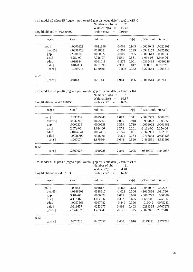
98
. ml model d0 d0pro15 (regco = poll over65 gnp dist educ dale ) / tau2 if c15>0 Number of obs = 21 Wald chi2(6) = 15.47Log likelihood = -60.680402 Prob > chi2 = 0.0169------------------------------------------------------------------------------------------------------------------- regco | Coef. Std. Err. z P>|z| [95% Conf. Interval]-------------------------------------------------------------------------------------------------------------------
poll | -.0000821 .0011848 -0.069 0.945 -.0024043 .0022401 over65 | -.0358928 .029808 -1.204 0.229 -.0943155 .0225298 gnp | -2.20e-07 .0000327 -0.007 0.995 -.0000643 .0000639 dist | 4.25e-07 7.72e-07 0.551 0.581 -1.09e-06 1.94e-06 educ | -.019984 .0061018 -3.275 0.001 -.0319434 -.0080246 dale | .0482014 .0201695 2.390 0.017 .00867 .0877328 _cons | -1.009914 1.130495 -0.893 0.372 -3.225644 1.205815-------------------------------------------------------------------------------------------------------------------tau2 | _cons | .04813 .025144 1.914 0.056 -.0011514 .0974113-------------------------------------------------------------------------------------------------------------------
. ml model d0 d0pro16 (regco = poll over65 gnp dist educ dale ) / tau2 if c16>0 Number of obs = 21 Wald chi2(6) = 10.87Log likelihood = -77.156455 Prob > chi2 = 0.0924------------------------------------------------------------------------------------------------------------------- regco | Coef. Std. Err. z P>|z| [95% Conf. Interval]-------------------------------------------------------------------------------------------------------------------
poll | .0030332 .0029945 1.013 0.311 -.0028359 .0089023 over65 | .0032268 .0495565 0.065 0.948 -.0939022 .1003558 gnp | .0000229 .0000638 0.359 0.719 -.0001022 .0001481 dist | 2.07e-06 1.62e-06 1.278 0.201 -1.11e-06 5.25e-06 educ | -.0164941 .0094415 -1.747 0.081 -.0349991 .002011 dale | -.0086707 .0316401 -0.274 0.784 -.0706842 .0533428 _cons | 1.207074 1.875864 0.643 0.520 -2.469551 4.883699-------------------------------------------------------------------------------------------------------------------tau2 | _cons | .2869027 .1010228 2.840 0.005 .0889017 .4849037-------------------------------------------------------------------------------------------------------------------
. ml model d0 d0pro17 (regco = poll over65 gnp dist educ dale ) / tau2 if c17>0Number of obs = 21
Wald chi2(6) = 4.40Log likelihood = -64.621635 Prob > chi2 = 0.6232------------------------------------------------------------------------------------------------------------------- regco | Coef. Std. Err. z P>|z| [95% Conf. Interval]-------------------------------------------------------------------------------------------------------------------
poll | -.0008413 .0018175 -0.463 0.643 -.0044037 .002721 over65 | -.0346601 .0338917 -1.023 0.306 -.1010866 .0317664 gnp | 3.18e-06 .0000423 0.075 0.940 -.0000797 .000086 dist | 4.11e-07 1.05e-06 0.392 0.695 -1.65e-06 2.47e-06 educ | -.0057568 .0067782 -0.849 0.396 -.019042 .0075283 dale | .0211657 .0253077 0.836 0.403 -.0284365 .0707678 _cons | -.1742026 1.453949 -0.120 0.905 -3.023891 2.675486-------------------------------------------------------------------------------------------------------------------tau2 | _cons | .0978215 .0407657 2.400 0.016 .0179221 .1777209-------------------------------------------------------------------------------------------------------------------
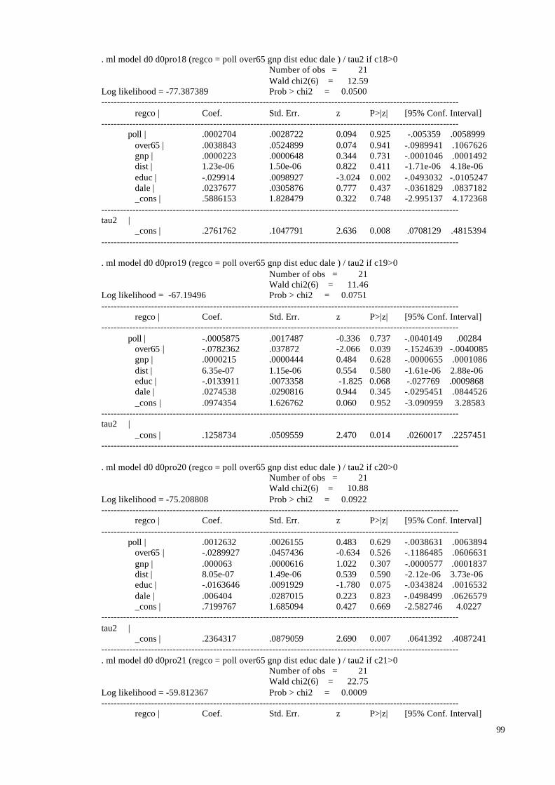
99
. ml model d0 d0pro18 (regco = poll over65 gnp dist educ dale ) / tau2 if c18>0 Number of obs = 21 Wald chi2(6) = 12.59Log likelihood = -77.387389 Prob > chi2 = 0.0500------------------------------------------------------------------------------------------------------------------- regco | Coef. Std. Err. z P>|z| [95% Conf. Interval]-------------------------------------------------------------------------------------------------------------------
poll | .0002704 .0028722 0.094 0.925 -.005359 .0058999 over65 | .0038843 .0524899 0.074 0.941 -.0989941 .1067626 gnp | .0000223 .0000648 0.344 0.731 -.0001046 .0001492 dist | 1.23e-06 1.50e-06 0.822 0.411 -1.71e-06 4.18e-06 educ | -.029914 .0098927 -3.024 0.002 -.0493032 -.0105247 dale | .0237677 .0305876 0.777 0.437 -.0361829 .0837182 _cons | .5886153 1.828479 0.322 0.748 -2.995137 4.172368-------------------------------------------------------------------------------------------------------------------tau2 | _cons | .2761762 .1047791 2.636 0.008 .0708129 .4815394-------------------------------------------------------------------------------------------------------------------
. ml model d0 d0pro19 (regco = poll over65 gnp dist educ dale ) / tau2 if c19>0 Number of obs = 21 Wald chi2(6) = 11.46Log likelihood = -67.19496 Prob > chi2 = 0.0751------------------------------------------------------------------------------------------------------------------- regco | Coef. Std. Err. z P>|z| [95% Conf. Interval]-------------------------------------------------------------------------------------------------------------------
poll | -.0005875 .0017487 -0.336 0.737 -.0040149 .00284 over65 | -.0782362 .037872 -2.066 0.039 -.1524639 -.0040085 gnp | .0000215 .0000444 0.484 0.628 -.0000655 .0001086 dist | 6.35e-07 1.15e-06 0.554 0.580 -1.61e-06 2.88e-06 educ | -.0133911 .0073358 -1.825 0.068 -.027769 .0009868 dale | .0274538 .0290816 0.944 0.345 -.0295451 .0844526 _cons | .0974354 1.626762 0.060 0.952 -3.090959 3.28583-------------------------------------------------------------------------------------------------------------------tau2 | _cons | .1258734 .0509559 2.470 0.014 .0260017 .2257451-------------------------------------------------------------------------------------------------------------------
. ml model d0 d0pro20 (regco = poll over65 gnp dist educ dale ) / tau2 if c20>0 Number of obs = 21 Wald chi2(6) = 10.88Log likelihood = -75.208808 Prob > chi2 = 0.0922------------------------------------------------------------------------------------------------------------------- regco | Coef. Std. Err. z P>|z| [95% Conf. Interval]-------------------------------------------------------------------------------------------------------------------
poll | .0012632 .0026155 0.483 0.629 -.0038631 .0063894 over65 | -.0289927 .0457436 -0.634 0.526 -.1186485 .0606631 gnp | .000063 .0000616 1.022 0.307 -.0000577 .0001837 dist | 8.05e-07 1.49e-06 0.539 0.590 -2.12e-06 3.73e-06 educ | -.0163646 .0091929 -1.780 0.075 -.0343824 .0016532 dale | .006404 .0287015 0.223 0.823 -.0498499 .0626579 _cons | .7199767 1.685094 0.427 0.669 -2.582746 4.0227-------------------------------------------------------------------------------------------------------------------tau2 | _cons | .2364317 .0879059 2.690 0.007 .0641392 .4087241-------------------------------------------------------------------------------------------------------------------. ml model d0 d0pro21 (regco = poll over65 gnp dist educ dale ) / tau2 if c21>0
Number of obs = 21 Wald chi2(6) = 22.75Log likelihood = -59.812367 Prob > chi2 = 0.0009------------------------------------------------------------------------------------------------------------------- regco | Coef. Std. Err. z P>|z| [95% Conf. Interval]

100
-------------------------------------------------------------------------------------------------------------------poll | .0001983 .0013292 0.149 0.881 -.002407 .0028035
over65 | -.0266413 .0272508 -0.978 0.328 -.080052 .0267693 gnp | .0000232 .0000298 0.777 0.437 -.0000353 .0000817 dist | -5.94e-07 6.93e-07 -0.857 0.391 -1.95e-06 7.65e-07 educ | -.0208296 .0054341 -3.833 0.000 -.0314802 -.010179 dale | .0535833 .0179492 2.985 0.003 .0184035 .0887631 _cons | -1.372144 1.061943 -1.292 0.196 -3.453514 .709226-------------------------------------------------------------------------------------------------------------------tau2 | _cons | .0379386 .0208807 1.817 0.069 -.0029867 .078864-------------------------------------------------------------------------------------------------------------------
. ml model d0 d0pro22 (regco = poll over65 gnp dist educ dale ) / tau2 if c22>0Number of obs = 21
Wald chi2(6) = 9.97Log likelihood = -79.175377 Prob > chi2 = 0.1259------------------------------------------------------------------------------------------------------------------- regco | Coef. Std. Err. z P>|z| [95% Conf. Interval]-------------------------------------------------------------------------------------------------------------------
poll | -.0006727 .0026079 -0.258 0.796 -.0057842 .0044387 over65 | -.0002732 .0512389 -0.005 0.996 -.1006996 .1001532 gnp | .0000286 .0000688 0.415 0.678 -.0001062 .0001634 dist | 8.58e-07 1.56e-06 0.550 0.582 -2.20e-06 3.91e-06 educ | -.0235602 .0100124 -2.353 0.019 -.0431841 -.0039362 dale | .0106132 .0318721 0.333 0.739 -.051855 .0730814 _cons | 1.223484 1.89204 0.647 0.518 -2.484846 4.931814-------------------------------------------------------------------------------------------------------------------tau2 | _cons | .293957 .1117149 2.631 0.009 .0749997 .5129142-------------------------------------------------------------------------------------------------------------------
. ml model d0 d0pro23 (regco = poll over65 gnp dist educ dale ) / tau2 if c23>0Number of obs = 21
Wald chi2(6) = 10.66Log likelihood = -67.786131 Prob > chi2 = 0.0995------------------------------------------------------------------------------------------------------------------- regco | Coef. Std. Err. z P>|z| [95% Conf. Interval]-------------------------------------------------------------------------------------------------------------------
poll | -.0012702 .0015677 -0.810 0.418 -.0043429 .0018025 over65 | -.0799726 .0324277 -2.466 0.014 -.1435298 -.0164154 gnp | .0000315 .0000409 0.771 0.441 -.0000486 .0001117 dist | -8.47e-08 1.09e-06 -0.077 0.938 -2.23e-06 2.06e-06 educ | -.012043 .0067827 -1.776 0.076 -.0253369 .001251 dale | .0357296 .0263827 1.354 0.176 -.0159796 .0874388 _cons | -.3160896 1.456501 -0.217 0.828 -3.170778 2.538599-------------------------------------------------------------------------------------------------------------------tau2 | _cons | .0962779 .044003 2.188 0.029 .0100336 .1825222-------------------------------------------------------------------------------------------------------------------. ml model d0 d0pro24 (regco = poll over65 gnp dist educ dale ) / tau2 if c24>0
Number of obs = 21 Wald chi2(6) = 10.80Log likelihood = -75.175338 Prob > chi2 = 0.0946------------------------------------------------------------------------------------------------------------------- regco | Coef. Std. Err. z P>|z| [95% Conf. Interval]-------------------------------------------------------------------------------------------------------------------
poll | .0025545 .0027103 0.942 0.346 -.0027577 .0078666 over65 | -.0359248 .0415632 -0.864 0.387 -.1173871 .0455376 gnp | .0000816 .0000603 1.353 0.176 -.0000366 .0001999 dist | 2.19e-07 1.46e-06 0.149 0.881 -2.65e-06 3.09e-06 educ | -.0204541 .0090793 -2.253 0.024 -.0382491 -.002659

101
dale | .0166926 .0280277 0.596 0.551 -.0382407 .0716259 _cons | .2262885 1.675956 0.135 0.893 -3.058524 3.511101-------------------------------------------------------------------------------------------------------------------tau2 | _cons | .2254896 .0866677 2.602 0.009 .055624 .3953552-------------------------------------------------------------------------------------------------------------------

102
Recommended