Using Maxent to Model the Distribution of Prehistoric Agricultural Features in a Portion of the Hōkūli‘a Subdivision in Kona, Hawai‘i
by
Solomon Ha‘aheo Kailihiwa, III
A Thesis Presented to the FACULTY OF THE USC GRADUATE SCHOOL
UNIVERSITY OF SOUTHERN CALIFORNIA In Partial Fulfillment of the
Requirements for the Degree MASTER OF SCIENCE
(GEOGRAPHIC INFORMATION SCIENCE AND TECHNOLOGY)
August 2015
Copyright 2015 Solomon Ha‘aheo Kailihiwa, III

ii
DEDICATION
For Juliana, my loving and supporting wife, and Savia, my reason for enduring.

iii
ACKNOWLEDGMENTS
This endeavor would not have been possible without a number of individuals that it has been my
honor to work with and to know. Dr. Patrick V. Kirch introduced me to the world of Hawaiian
archaeology, without Uncle Pat, I would not be where I am today. Dr. Paul L. Cleghorn
provided me the opportunity to live and to do archaeology in Hawai‘i, he never gave up hope
that I would someday attend graduate school. Dr. Alan E. Haun provided the opportunity and
support for me to work on this project. Thank you also goes to Dr. Thomas Garrison and Dr. Su
Jin Lee for being on my committee and offering valuable input and advice. Dr. Karen Kemp
provided invaluable guidance throughout the thesis process. To my parents, Solomon and
Audreen Kailihiwa, for building the foundation of my successes. Thank you to Joseph and Carol
Vivona whose support helped to keep the torch alive. Last, and definitely not least,
immeasurable gratitude to Juliana Kailihiwa for her support and for putting up with me during
this research.
iv
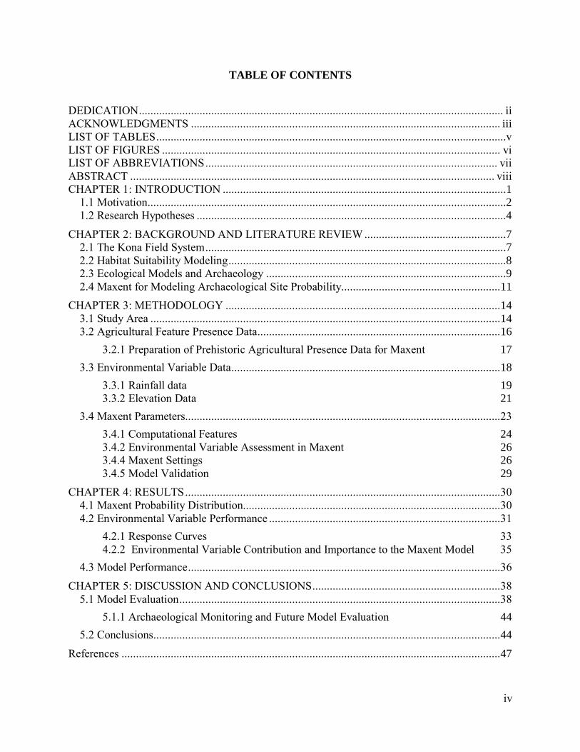
TABLE OF CONTENTS
DEDICATION .............................................................................................................................. ii ACKNOWLEDGMENTS ........................................................................................................... iii LIST OF TABLES .........................................................................................................................v LIST OF FIGURES ..................................................................................................................... vi LIST OF ABBREVIATIONS ..................................................................................................... vii ABSTRACT .............................................................................................................................. viii CHAPTER 1: INTRODUCTION ..................................................................................................1
1.1 Motivation ............................................................................................................................2 1.2 Research Hypotheses ...........................................................................................................4
CHAPTER 2: BACKGROUND AND LITERATURE REVIEW .................................................7 2.1 The Kona Field System ........................................................................................................7 2.2 Habitat Suitability Modeling ................................................................................................8 2.3 Ecological Models and Archaeology ...................................................................................9 2.4 Maxent for Modeling Archaeological Site Probability....................................................... 11
CHAPTER 3: METHODOLOGY ............................................................................................... 14 3.1 Study Area ......................................................................................................................... 14 3.2 Agricultural Feature Presence Data .................................................................................... 16
3.2.1 Preparation of Prehistoric Agricultural Presence Data for Maxent 17
3.3 Environmental Variable Data ............................................................................................. 18
3.3.1 Rainfall data 19 3.3.2 Elevation Data 21
3.4 Maxent Parameters............................................................................................................. 23
3.4.1 Computational Features 24 3.4.2 Environmental Variable Assessment in Maxent 26 3.4.4 Maxent Settings 26 3.4.5 Model Validation 29
CHAPTER 4: RESULTS ............................................................................................................. 30 4.1 Maxent Probability Distribution......................................................................................... 30 4.2 Environmental Variable Performance ................................................................................ 31
4.2.1 Response Curves 33 4.2.2 Environmental Variable Contribution and Importance to the Maxent Model 35
4.3 Model Performance ............................................................................................................ 36
CHAPTER 5: DISCUSSION AND CONCLUSIONS ................................................................. 38 5.1 Model Evaluation ............................................................................................................... 38
5.1.1 Archaeological Monitoring and Future Model Evaluation 44
5.2 Conclusions ........................................................................................................................ 44
References ................................................................................................................................... 47
v
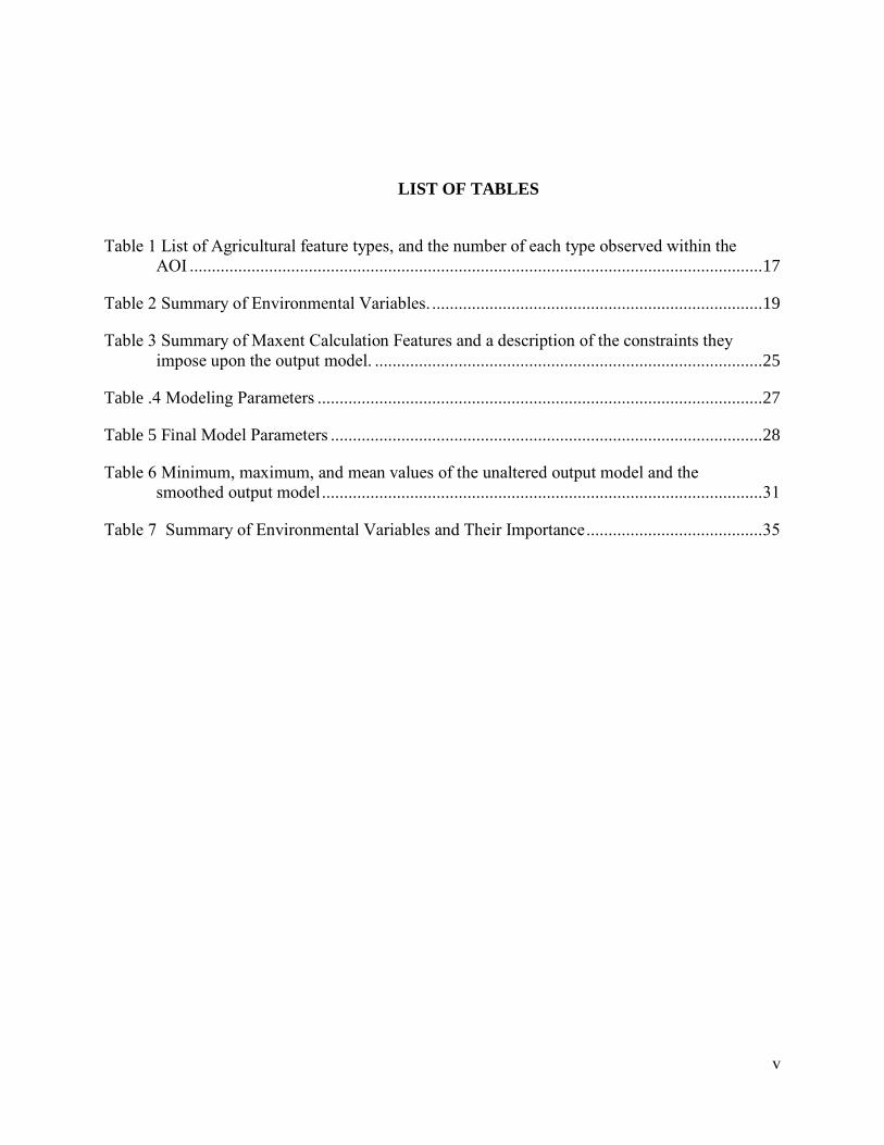
LIST OF TABLES
Table 1 List of Agricultural feature types, and the number of each type observed within the AOI .................................................................................................................................. 17
Table 2 Summary of Environmental Variables. ........................................................................... 19
Table 3 Summary of Maxent Calculation Features and a description of the constraints they impose upon the output model. ........................................................................................ 25
Table .4 Modeling Parameters ..................................................................................................... 27
Table 5 Final Model Parameters .................................................................................................. 28
Table 6 Minimum, maximum, and mean values of the unaltered output model and the smoothed output model .................................................................................................... 31
Table 7 Summary of Environmental Variables and Their Importance ........................................ 35
vi
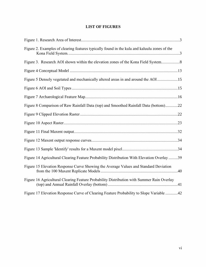
LIST OF FIGURES
Figure 1. Research Area of Interest. ...............................................................................................3
Figure 2. Examples of clearing features typically found in the kula and kaluulu zones of the Kona Field System. ............................................................................................................3
Figure 3. Research AOI shown within the elevation zones of the Kona Field System ..................8
Figure 4 Conceptual Model ......................................................................................................... 13
Figure 5 Densely vegetated and mechanically altered areas in and around the AOI .................... 15
Figure 6 AOI and Soil Types ....................................................................................................... 15
Figure 7 Archaeological Feature Map .......................................................................................... 16
Figure 8 Comparison of Raw Rainfall Data (top) and Smoothed Rainfall Data (bottom) ............ 22
Figure 9 Clipped Elevation Raster ............................................................................................... 22
Figure 10 Aspect Raster ............................................................................................................... 23
Figure 11 Final Maxent output ..................................................................................................... 32
Figure 12 Maxent output response curves. ................................................................................... 34
Figure 13 Sample 'Identify' results for a Maxent model pixel ...................................................... 34
Figure 14 Agricultural Clearing Feature Probability Distribution With Elevation Overlay ......... 39
Figure 15 Elevation Response Curve Showing the Average Values and Standard Deviation from the 100 Maxent Replicate Models ........................................................................... 40
Figure 16 Agricultural Clearing Feature Probability Distribution with Summer Rain Overlay (top) and Annual Rainfall Overlay (bottom) .................................................................... 41
Figure 17 Elevation Response Curve of Clearing Feature Probability to Slope Variable ............ 42

vii
LIST OF ABBREVIATIONS
AIS Archaeological inventory survey
AOI Area of Interest
ASCII American Standard Code for Information Interchange
AUC Area under the receiver operator curve
CPU Central Processing Unit
DLNR Department of Land and Natural Resources
.dxf Drawing Exchange Format
ENFA Ecological niche factor analysis
GARP Genetic Algorithm for Rule-Set Prediction
GPS Global Positioning System
GUI Graphical user interface
HTML Hypertext markup language
NAD83 North American Datum 1983
PRISM Parameter-elevation Regressions on Independent Slopes Model
ROC Receiver operator characteristics
ROR Relative occurrence rate
SHPD State Historic Preservation Division
UTM Universal Transverse Mercator
WGS1984 World Geodetic System 1984

viii
ABSTRACT
Archaeological investigations are an integral part of the permitting process for land development
in Hawai‘i. The State recognizes that conservation of its historic and cultural heritage is
important and that its cultural resources are nonrenewable. A recent archaeological survey for
prehistoric and historic agricultural features in the Hōkūli‘a luxury development on Hawai‘i
Island afforded an opportunity to test maximum entropy theory as a method for predicting the
presence of archaeological features. The Maxent computer program uses a machine learning
algorithm that utilizes presence point data and environmental variable rasters to produce a
probability distribution of the species of interest. The "species" of interest for this research were
agricultural clearing features, associated with sweetpotato (Ipomea batatas) cultivation,
identified in a portion of Hōkūli‘a which lies within the Kona Field System. Previous
agricultural habitat suitability models for Hawai‘i were used to determine the environmental
variables used in this research; the variables included annual rainfall, summer rainfall, elevation,
and slope. Maxent produced a probability distribution that matched the expectations of the
conceptual model. The model was validated using diagnostic tools included in the Maxent
program (1) area under the receiver operator characteristic curve analysis, (2) jack-knife testing,
and (3) environmental variable response curve analysis, as well as three research hypotheses.
The model does not account for human behavior and may overestimate feature presence in
uncultivated, spiritually important areas that are suitable for farming. The results of this research
show that Maxent can be used to successfully model certain types archaeological features.

1
CHAPTER 1: INTRODUCTION
Archaeological inventory surveys are the primary method used to identify historic and
prehistoric resources throughout the State of Hawai‘i on lands that are slated for development.
This research focuses on an archaeological investigation conducted within Hōkūli‘a, a luxury
subdivision that spans 10 ahupua‘a (traditional land divisions) located along the western shore of
Hawai‘i Island in the North Kona and South Kona Districts within an area known as the Kona
Field System, an area of intense prehistoric agricultural production (Allen 2001a; Allen 2004).
Archaeological investigations have been conducted within Hōkūli‘a beginning in 1930 and
resuming in 1988 through the present (Tomonari-Tuggle and Tuggle 2008). An archaeological
survey of prehistoric agricultural features undertaken in 2014-15, requested by the Hawai‘i State
Historic Preservation Division (SHPD) of the Department of Land and Natural Resources
(DLNR), in the Hōkūli‘a subdivision, provided an opportunity to test the use of the maximum
entropy model as a means for creating a probability distribution of archaeological features in
areas where it is not possible to conduct a comprehensive survey.
The area of interest (AOI) is an approximate 312-acre portion of the Hōkūli‘a
Subdivision. Figure 1 shows the AOI and its location within the larger extent of the Kona Field
System. The archaeological survey crew was unable to record agricultural features in portions of
the AOI covered by dense, impenetrable vegetation and areas altered by heavy machinery.
Stands of dense guinea grass (Megathyrsus maximus) are located throughout the property
obscuring the ground surface and impeding pedestrian survey. Much of the area has also been
mechanically altered by heavy equipment and prehistoric agricultural features have been
removed from the landscape. The objective of this research is to use Maxent to model a
probability distribution of agricultural clearing features.

2
1.1 Motivation
The need to provide statistical support for conclusions derived from the data collected
during the ongoing fieldwork motivated this research. Maxent has been used successfully in
species distribution modeling (Merow, Smith, and Silander 2013) and is able to create reliable
models with a limited number of presence-only samples (Phillips, Anderson, and Schapire 2005;
Elith et al. 2011; Merow, Smith, and Silander 2013). The Maxent modeling program was used to
produce a probability distribution of prehistoric agricultural features in mechanically disturbed
and densely vegetated areas within the AOI based on the observed presence data and
environmental variables. Habitat suitability modeling and maximum entropy theory were used
to model the probability distribution of the agricultural features.
Habitat suitability modeling considers the relationship between environmental variables
and the probability that a given species will occur (Hirzel and Le Lay 2008). Maximum entropy
uses only observed occurrences of a species to create a probability distribution (Roxburgh and
Mokany 2010). The Maxent program developed by Phillips, Dudík, and Schapire (2004) creates
a probability distribution using presence-only data and environmental variables. The “species”
of interest for this study were the agricultural clearing features, rock mounds and modified
outcrops, most commonly found within the kula and kaluulu zones of the Kona Field System.
Figure 2 shows examples of the clearing features typically found within the AOI.
The Kona Field System is characterized by four distinct planting zones defined by
elevation (Newman 1971; Kelly 1983): kula (coast— 500 ft), kaluulu (500—1,000 ft), ‘āpa‘a
(1,000—2,500 ft), and ‘ama‘u (2,000—3,000 ft). The habitat for the agricultural features was
defined by the environmental variables discussed in previous archaeological reports and
historical accounts: elevation, slope, and rainfall (Newman 1971; Kelly 1983; Allen 2001b).

3
Figure 1. Research Area of Interest. An estimated extent of the Kona Field System is shown in brown in the inset map.
Figure 2. Examples of clearing features typically found in the kula and kaluulu zones of the Kona Field System. A modified outcrop is shown on the left, a rock mound on the right.

4
The general conceptual model for this research is that the density of the rock mounds and
modified outcrops will be relatively sparse along the coastal area and feature density will
increase with the rise in elevation up to the ‘āpa‘a zone where the Kona Field System is a more
formal collection of walled fields (Allen 2001b).
The validity of this model was determined through statistical tests that are included as
part of the Maxent program and ground truthing. These tests include binomial tests of omission
and the area under the receiver operator curve value (AUC) analysis, which were used to
determine the goodness of fit for the Maxent outputs. Jack-knife testing, which assesses the
contribution of each environmental variable to the model, and response curves, which show how
the model responds to the environmental variables, are also available within Maxent. These tests
and three research hypotheses were used to evaluate the model produced by Maxent.
1.2 Research Hypotheses
Three research hypotheses were developed to evaluate the Maxent output model. The
first hypothesis states that clearing feature (rock mounds and modified outcrops) density
increases as one ascends from the shoreline to the upper elevations of the kula zone and the
lower elevation of the kaluulu zone. Clearing feature density should decrease starting in the mid-
elevations of the kaluulu zone.
This hypothesis is based on the results of an archaeological inventory survey (AIS)
conducted approximately three kilometers to the north of the current AOI by Haun and Henry
(2010). Their findings indicated that the feature density was greatest between the elevations of
360 ft and 680 ft which corresponds to the upper elevations of the kula zone and the lower
elevations of the kaluulu zone. Clearing feature density began to decrease at elevations higher

5
than 680 ft and dropped even more at the upper elevations of the kaluulu zone as agricultural
features and methods become more formalized in the āpa‘a zone.
The second hypothesis states that as precipitation levels approach acceptable levels for
dryland taro farming, there is a decrease in the density of informal clearing features that are used
in sweetpotato1 cultivation.
Sweetpotato requires much less water than taro (Colocasia esculenta) which is why the
sweetpotato was cultivated so intensely in the dry lowlands of the Kona Field System (Handy,
Handy, and Pukui 1991). There should be a decrease in the informal agricultural features as
precipitation increases to levels where formal, rain-fed, dryland agriculture is sustainable.
Ladefoged et al. (2009) stated that the annual precipitation required for optimal sweetpotato
cultivation was 750—1000 mm.
The third hypothesis states that agricultural practices were limited to slopes less than 35
percent; most agriculture took place on slopes less than 20 percent.
Newman (1971) conducted an analysis of the environmental characteristics of the
agricultural areas on Hawai‘i Island that were observed by Reverend William Ellis during his
tour of the island in 1823. Newman created a number of generalizations of the environmental
variables which included annual mean rainfall, elevation, slope, drainage, soil parent material,
and soil type. Newman generalized that the agricultural zones for Hawai‘i Island incorporated
areas that had a slope less than 35 percent with the majority having a slope less than 20 percent.
The following chapters describe the work and findings of this research. Chapter 2
provides background on habitat suitability modeling, the Maxent modeling program, and
ecological models used in an archaeological context. Chapter 3 discusses the preparation of the
presence data and environmental variable rasters, and the parameters used in Maxent. Chapter 4 1 Valenzuela, Fukuda and Arakaki (2000) explicitly state, "Sweetpotato is, in fact, one word..."

6
discusses the model, its response to the environmental variables, and the methods used to
evaluate the model. Chapter 5 discusses the conclusions drawn from the results, improvements
that could be made to the model, and future uses of Maxent in the Kona Field System.

7
CHAPTER 2: BACKGROUND AND LITERATURE REVIEW
Ecological models have been applied to Hawai‘i in efforts to identify areas suitable for
agricultural production. This chapter discusses the Kona Field System, habitat suitability
modeling, the Maxent program, and the implications of using environmental variables to model
archaeological resources which are the result of human behavior which is not determined by
environmental variables.
2.1 The Kona Field System
The Kona Field System is a rain-fed agricultural system located in the Kona District on
the leeward, west, side of Hawai‘i Island (Allen 2001a; Allen 2004; Cordy 2000; Kelly 1983;
Lincoln and Ladefoged 2014). The Kona Field System was described by early visitors to
Hawai‘i Island (Ellis 1917; Ledyard 1963; Menzies 1920) and Māhele land claim testimonies
(Kelly 1983; Lincoln and Ladefoged 2014; Cordy 2000). The main crops cultivated within the
Kona Field System included wauke (paper mulberry [Broussonetia papyrifera]), ‘uala
(sweetpotato [Ipomea batatas]), ‘ulu (breadfruit [Autocarpus altilis]), kalo (taro [Colocasia
esculenta]), kō (sugar cane [Saccharum officinarum]), kī (ti [Cordyline terminalis]), mai‘a
(banana [Musa spp.]), and ‘ama‘u (endemic tree ferns [Sadleria spp.]) (Allen 2001a; Kelly 1983;
Lincoln and Ladefoged 2014; Cordy 2000).
The Kona Field System was divided into four different zones which were determined by
elevation and rainfall (Handy, Handy, and Pukui 1991; Kelly 1983). Kelly defines these zones
as kula (0—500 ft), kaluulu (500—1,000 ft), ‘āpa‘a (1,000—2,500 ft), and ‘ama‘u (2,000—
3,000 ft). Figure 3 shows that the AOI for this research lies within the lower three elevation
zones with the majority of the area in the kula and kaluulu zones. ‘Uala (sweetpotato) was the

8
main crop of the kula zone, ‘ulu (breadfruit) was the main crop within the kaluulu zone
(Newman 1971; Kelly 1983; Lincoln and Ladefoged 2014).
Figure 3. Research AOI shown within the elevation zones of the Kona Field System
2.2 Habitat Suitability Modeling
Habitat suitability modeling considers the relationship between environmental variables
and the probability that a given species will occur (Hirzel and Le Lay 2008). Habitat suitability
modeling provides a method of predicting the species occurrence where there is little
observational data available on the species of interest (Pearson et al. 2007). Pearson et al. (2007)
do caution that modeling species occurrence with limited presence data identifies regions that
have characteristics similar to those where the species occur and not the limits of that species'
habitat range.
Phillips, Dudík, and Schapire (2004) propose the use of maximum entropy to model
species geographic distributions. The maximum entropy method for modeling species
distribution involves using a collection of known species localities as sample data along with
relevant environmental factors to model the distribution of that species within a known

9
geographic extent (Phillips, Dudík, and Schapire 2004). Phillips, Anderson, and Schapire (2005)
describe the use and testing of the Maxent program, a widely used maximum entropy modeling
toolbox, to model species geographic distributions using habitat suitability, and presence-only
data. They assess their resulting models' validity using binomial tests of omission and receiver
operator characteristics (ROC) analysis. Elith, et al. (2011) describes how to use the Maxent
modeling program and makes suggestions for which parameters should be used.
Anderson, Lew, and Peterson (2003) deal with evaluating the validity of predictive
models of species' distributions. While they use the Genetic Algorithm for Rule-Set Prediction
(GARP), their article is pertinent because their study applies to stochastic models that use
presence-only data. They propose a method for determining an optimal
underestimation/overestimation of presence (omission/commission) relationship to select models
that reasonably predict the distribution of a species.
Haegeman and Loreau (2008) caution against the blind use of maximum entropy theory
in ecology. They show that the restrictive constraints may dictate the outputs of maximum
entropy modeling and cause the models to over-fit the probability distributions to the presence-
only data. In order for maximum entropy to be effective in ecological modeling, the
environmental variables must be understood and carefully chosen (Haegeman and Loreau 2008).
2.3 Ecological Models and Archaeology
The Kona Field System has previously been spatially modeled as either general models
of agriculture in Hawai‘i (Ladefoged et al. 2009) or concentrated on the extent of the kaluulu
zone (Lincoln and Ladefoged 2014). Ladefoged et al (2009) created a model of the two main
different types of agricultural systems throughout the state of Hawai‘i: irrigated pondfields and
rain-fed dryland systems. They used three variables important in sweetpotato cultivation,
10
rainfall, elevation, and soil fertility, to model the rain-fed dryland agriculture systems. This
model of rain-fed dryland agricultural systems successfully predicted the leeward Kohala field
system on Hawai‘i Island and the Kalaupapa field system on Moloka‘i. It also under-predicted
the presence of the Kona Field System. Discrepancies between the model and observed
agricultural development were explained by the presence of variables that were difficult to
quantify and could not be accounted for in an ecological model (Ladefoged et al. 2009).
Lincoln and Ladefoged (2014) modeled the extent and potential yield of the kaluulu zone
using historic descriptions and archaeological survey. Rainfall and elevation rasters were used to
determine the environmental boundaries of the kaluulu zone in their model. Lincoln and
Ladefoged’s model increased the previously estimated extent and size of the kaluulu zone.
Such previous studies on Hawai‘i Island have modeled the extent and yield of the Kona
Field System, but they have not looked at the potential distribution of features within the field
system. They have utilized habitat suitability modeling, but not maximum entropy. Two more
examples of ecological models in archaeology that have used presence-only data with
environmental variables are described below. The first was a project in Southern Italy modeling
probability distributions of Bronze Age sites and the second was a project using Maxent in
Cyprus to predict the presence of ancient and modern terraces.
Arnese (2008) used ecological niche factor analysis (ENFA) to create a probability
distribution of Bronze Age sites in Kaulonia located in Calabria, Southern Italy. ENFA utilizes
presence data and "eco-geographical" variables to model animal distributions (Arnese 2008).
The eco-geographical variables used in Arnese's model were elevation, distance from the sea,
slope, aspect, and distance from rivers. The ENFA model ranked elevation as the most important
variable followed by distance from the sea. Arnese was able to ground truth the model with

11
success. Areas with a high Habitat Suitability value contained Bronze Age sites and areas with a
low Habitat Suitability value did not contain any Bronze Age Sites.
Galletti et al. (2013) used Maxent successfully to model predictive distributions for
ancient and modern terraces in the Troodos foothills on the island of Cyprus. They used 10
environmental variables in their terrace probability distribution modeling. These variables
included, elevation, spring vegetation, fall vegetation, distance to nearest calcareous sediments,
distance to nearest major stream, slope, albedo, radiation, distance to nearest pillow lava, and
temperature. The AUC analysis, model gain, performance gain, and the Kvamme gain statistic
were used to evaluate the performance of their Maxent outputs. Galletti et al. were able to show
that the distributions of the ancient and modern terraces were determined differently by the
environmental variables.
2.4 Maxent for Modeling Archaeological Site Probability
The Maxent program2 uses maximum entropy theory to create a probability distribution
of a given species related to a series of environmental variables (Phillips, Dudík, and Schapire
2004; Phillips, Anderson, and Schapire 2005; Phillips and Dudík 2008). Maximum entropy
theory uses partial information, presence-only data, to create a probability distribution that best
conforms to a set of constraints, environmental variables, without considering any other
constraints (Jaynes 1957; Phillips, Dudík, and Schapire 2004).
The Maxent program developed by Phillips, Dudík, and Schapire (2004) is a machine
learning process that uses multiple iterations to train the model into creating an acceptable
model. Due to the stochastic nature of this process, multiple replicates of the model must be run
in order to bring the average of the outputs to a suitable result (Kemp 2012).
2 Available for download at http://www.cs.princeton.edu/~schapire/maxent/

12
Maxent requires a point dataset that contains the observed species occurrence, presence-
only, data and environmental raster datasets. In the case of the model described here, the
observed species data contains the coordinate information for each agricultural feature recorded
during the archaeological agriculture feature survey. The environmental variables for this study
were determined by previous studies that modeled rain-fed agricultural systems on Hawai‘i
Island (Newman 1971; Ladefoged et al. 2009; Lincoln and Ladefoged 2014). Newman (1971),
Ladefoged et al. (2009) and Lincoln and Ladefoged (2014) identify the environmental variables
used to determine the extent of rain-fed agriculture in the Kona Field System. These variables
include rainfall, elevation, slope, and soil fertility.
Within the Kona Field System, precipitation increases with elevation. The conceptual
model for this research proposes that agricultural clearing feature density increases with
increases in elevation and rainfall until taro cultivation is viable. At that point, farming methods
were more formalized in well defined fields and the less structured agricultural clearing feature
density declines. The conceptual model is shown in Figure 4 illustrating the increase and
decrease in rainfall and agricultural clearing feature density.
However, it is important to remember that agriculture is a human activity, and that human
behavior may not be dictated completely by the environment (Freilich 1967). Ecological
models can be used to identify the potential probability of archaeological feature presence based
on environmental variables but the models must be evaluated with empirical observations
(Ladefoged et al. 2009). The variables that define a spiritually important place cannot always be
quantified in a tangible manner (King 2003). An ecological model's inability to account for
intangible variables may cause the model to overestimate agricultural feature presence.

13
Figure 4 Conceptual Model
The next chapter discusses the preparation of the data and the Maxent model and the tests
used to evaluate the model.

14
CHAPTER 3: METHODOLOGY
Maxent creates a probability distribution model by using presence point data and environmental
variable raster grids. This chapter discusses the geographic extent of the model and the AOI, the
preparation of the agricultural presence data and environmental variable rasters, the Maxent
model setup, and finally the diagnostic tools built within the Maxent program that were used to
evaluate the final model.
3.1 Study Area
As previously described in Chapter 1, the AOI is an approximately 312-acre portion of
the Hōkūli‘a luxury development as shown in Figure 1. The AOI is approximately 3,235 m long,
and 1,430 m at its widest. Unfortunately, heavy machinery has altered portions of the AOI to an
extent where agricultural features were either completely removed from the landscape or altered
to such an extent that the features were not identifiable; thus, it was observed that agricultural
features were recorded with less frequency in mechanically altered areas. Dense stands of
guinea grass also prevented the crew from being able to survey portions of the AOI. Therefore,
predicting the distribution of agricultural features in these incompletely surveyed areas is the
main objective of this research. Figure 5 shows the AOI as well as the mechanically altered
portions and the densely vegetated areas.
The study area is situated on a recent pahoehoe flow, thus only one soil type covers the
majority of the AOI as shown in Figure 6. This led to the exclusion of soil attributes in this
model, as discussed below in Section 3.3 Environmental Variable Data.

15
Figure 5 Densely vegetated and mechanically altered areas in and around the AOI
Figure 6 AOI and Soil Types

16
3.2 Agricultural Feature Presence Data
Prehistoric and historic agricultural feature spatial and attribute data were collected
between the months of August 2014 and March 2015 (Kailihiwa 2015). The agricultural feature
data points are shown in Figure 7. The agricultural feature types included clearing features (rock
mounds and modified outcrops), agricultural terraces, grow pits, linear rock mounds, agricultural
enclosures, retaining walls, and swales; these are summarized in Table 1. Linear rock mounds,
agricultural enclosures, retaining walls, and swales were not used in this test of Maxent because
of the small number of observed occurrences for each feature. The clearing features, grow pits,
and agricultural terraces were each modeled separately. Linear mounds, even though they were
the second most numerous feature recorded, were not used to create a model because they are
line features and Maxent requires the presence data to be point features.
Figure 7 Archaeological Feature Map

17
Table 1 List of Agricultural feature types, and the number of each type observed within the AOI (Kailihiwa 2015)
Type Count
Clearing Feature 3743 Linear Mounds 139 Grow Pit 104 Terrace 89 Enclosure 42 Swale 2
Retaining Wall 1
The data was collected by a crew of archaeologists systematically surveying and
recording agricultural features within the AOI. The crew members were spaced five to ten
meters apart (spacing was dependent upon ground visibility) during the survey; spatial data was
recorded with handheld Global Positioning System (GPS) devices that provided an accuracy of
five to ten meters.
The central area of the AOI contained the densest concentration of agricultural feature
observed presences. This portion of the AOI was the least vegetated and the least impacted by
heavy machinery and provided the most accurate picture of agricultural feature distribution in the
entire AOI. The presence samples were not reduced in the area for modeling purposes, even
though they undoubtedly influenced the output probability distribution, because this region did
represent an unaltered view of agricultural feature intensity in the Kona Field System.
3.2.1 Preparation of Prehistoric Agricultural Presence Data for Maxent
Maxent requires that the presence data is in a comma delimited value text file that
contains three fields, at a minimum, that identify the "species," the X-coordinates and Y-
coordinates. The X and Y-coordinate values for each datum point were added to the attribute

18
table of the original presence point dataset. The values for each environmental variable were
also added to the attribute table for each sample point. The addition of the environmental
variable values ensured that Maxent would run more efficiently because it would not have to go
through each environmental raster to determine the values for each sample presence point
(Phillips n.d.). Once the pertinent data was added to the attribute table, it was converted to a
comma delimited text file.
3.3 Environmental Variable Data
Maxent requires that each of the environmental variables is stored in ASCII grid format
with all rasters sharing the same exact cell size and the same exact geographic extent. The
presence-only data must be in a comma delimited value table with a minimum of three fields
which denote species, X-coordinates and Y-coordinates. It is possible to set up Maxent once the
presence-only data and the environmental variable rasters are in the proper format.
As discussed in Chapter 2, Ladefoged et al. (2009), Lincoln and Ladefoged (2014), and
Newman (1971) identify the environmental variables that help to define the extent of the rain-fed
agriculture of the Kona Field System. These variables, which include rainfall, elevation, slope,
and soil fertility, are summarized in Table 2. The archaeological survey that generated the
presence-only data was conducted on a single soil type, pahoehoe bedrock (see Figure 6). Test
runs with soil fertility variables in Maxent showed that the model over-fit the probability
distribution to the soil polygon. Haun and Henry (2010) demonstrated that the soil in the region
is rocky enough that agricultural clearing features do occur on soil types other than pahoehoe
flows. Therefore, soil data were not used in the final model so that the probability distribution
created by Maxent would extend beyond the immediate boundaries of the archaeological survey

19
area. This section discusses each of the environmental datasets and their preparation for use in
Maxent.
Table 2 Summary of Environmental Variables. These variabels were identified in previous models of prehistoric agriculture in Hawai‘i and were used during test model runs.
Environmental Variable Content Format Comments
Elevation Elevation data Raster in ASCII grid format
Two foot elevation contour dataset converted to a raster grid with a cell size of 10 m. Source: Belt Collins, 2002, aerial survey
Slope Slope data derived from elevation data
Raster in ASCII grid format
Slope in percent rise with a cell size of 10 m. Derived from the elevation raster
Aspect Aspect raster derived from elevation data
Raster in ASCII grid format Derived from the elevation raster
Rainfall Data: Annual Average Summer Average Average totals for June, July, August, and September
Average yearly rainfall totals and average totals for summer months
Raster in ASCII grid format
30 year average rain totals. Original Cell size is 250 m. Raster grids Resampled to 10 m cell size to match the elevation and slope data. Projected from WGS84 to NAD83 UTM zone 5N; Source: Giambelluca et al. 2013
3.3.1 Rainfall data
The timing of the rainfall and the rainfall totals are important factors in sweetpotato
cultivation. Handy, Handy, and Pukui (1991) state that the best time to plant sweet potato in
Kona is during the summer months. Valenzuela, Fukuda, and Arakaki (2000) define the
tolerable rainfall range for sweetpotato during its growth cycle to be 500 to 1300 mm. While
rainfall datasets that cover the period of occupation for the Kona Field System are not readily
available, long-term modern rainfall data was available from Giambelluca et al. (2013).
The rainfall data3 available from Giambelluca et al. (2013) covers seven of the eight
principal Hawaiian Islands, Ni‘ihau is excluded from this dataset. The datasets are rasters with a
cell size of approximately 250 m x 250 m in the World Geodetic System 1984 (WGS1984)
geographic coordinate system. Giambelluca et al. (2013) used raingage data and expert
3 Available for download from http://rainfall.geography.hawaii.edu/downloads.html

20
knowledge supplemented by five predictors to create this data set. The five predictors included
updated raingage data with values averaged over 30 years from 1978--2007, Parameter-elevation
Regressions on Independent Slopes Model (PRISM) data for the years 1971—2000, National
Weather Service mean radar rainfall estimates, mean rainfall estimates created by experimental
model forecasts, and vegetation distribution (Giambelluca et al. 2013). Thirteen grids are
included in the dataset, an annual grid and a grid for each month.
The rainfall data from Giambelluca et al. (2013) that were selected for use in this model
included annual, June, July, August, and September totals averaged over a 30 year time period
from 1978—2007. This data is not contemporaneous with the Kona Field System occupation,
but it does show the expected pattern of rainfall increasing with elevation as well as rainfall
totals during the summer months in Kona, which, as mentioned above, were important for the
cultivation of sweetpotato in the region.
3.3.1.1 Rainfall Data Preparation
The rainfall datasets were downloaded from the Rainfall Atlas of Hawai‘i site in the Esri
grid format. The original data had a cell size of 250 m in the World Geodetic System 1984
(WGS1984) geographic coordinate system. The dataset was projected into the North American
Datum 1983 (NAD83) Universal Transverse Mercator (UTM) zone 5 North (5N) projected
coordinate system. As can be seen in Figure 8 top, these large cells produce a blocky appearance
at the scale of the study area. Since rainfall is a continuous phenomenon, it was decided that it
was appropriate to smooth this data as they were projected and resized to the model's
computational scale of 10 m. The rainfall grids were smoothed using bilinear interpolation
which averages the four nearest input cells weighted by their distance to the center of the input
raster cell (Esri 2009). This resulted in a surface with gradually increasing rainfall amounts over

21
smaller-sized cells rather than the sudden jumps in values with the coarser dataset (see Figure 8
bottom). Once the rainfall data was projected and resized it was clipped and converted to an
ASCII grid, ready for use in Maxent.
3.3.2 Elevation Data
Since a fine resolution elevation grid was not available, an AutoCAD Drawing Exchange
Format (.dxf) file containing 2 ft contour lines of the Hōkūli‘a property provided the elevation
data. This data was derived from an aerial photogrammetry survey flown in 2002 and has an
expected vertical accuracy of two meters. The vertical accuracy was affected by the height of
the guinea grass covering the ground in the survey area. After converting the lines into a
shapefile containing a line feature class, non-elevation lines were removed and elevation values
were assigned to each contour line. The .dxf file was in the Old Hawaiian State Plane Hawaii 1
projected coordinate system and was reprojected to the NAD83 UTM zone 5N projected
coordinate system. Once the file was reprojected it was then georeferenced to the World
Imagery basemap available in ArcGIS 10.2.2, which has an horizontal accuracy of 10 m. With
the conversion from CAD to GIS data complete, it was possible to create the elevation raster.
3.3.2.1 Elevation and Elevation Derived Rasters
The elevation contours were interpolated into a raster using the assigned values, in feet,
of each line to determine the value of each cell. The cell size was set to 10 m by 10 m. A mask
that followed the outline of the elevation contour shapefile was used to clip the elevation raster to
limit the model's calculation to the area in which the elevation was known. This same mask was
used to clip all of the environmental variables to a common spatial extent. Figure 9 shows the
elevation raster clipped to the model's spatial extent.

22
Figure 8 Comparison of Raw Rainfall Data (top) and Smoothed Rainfall Data (bottom)
Figure 9 Clipped Elevation Raster
23
The elevation raster was used to create a slope raster. The cell size and extent of the
slope raster were set to the same values as the elevation raster. The output measurement for the
slope raster was set to percent rise due to the slope variables (percentage) discussed in Newman
(1971).
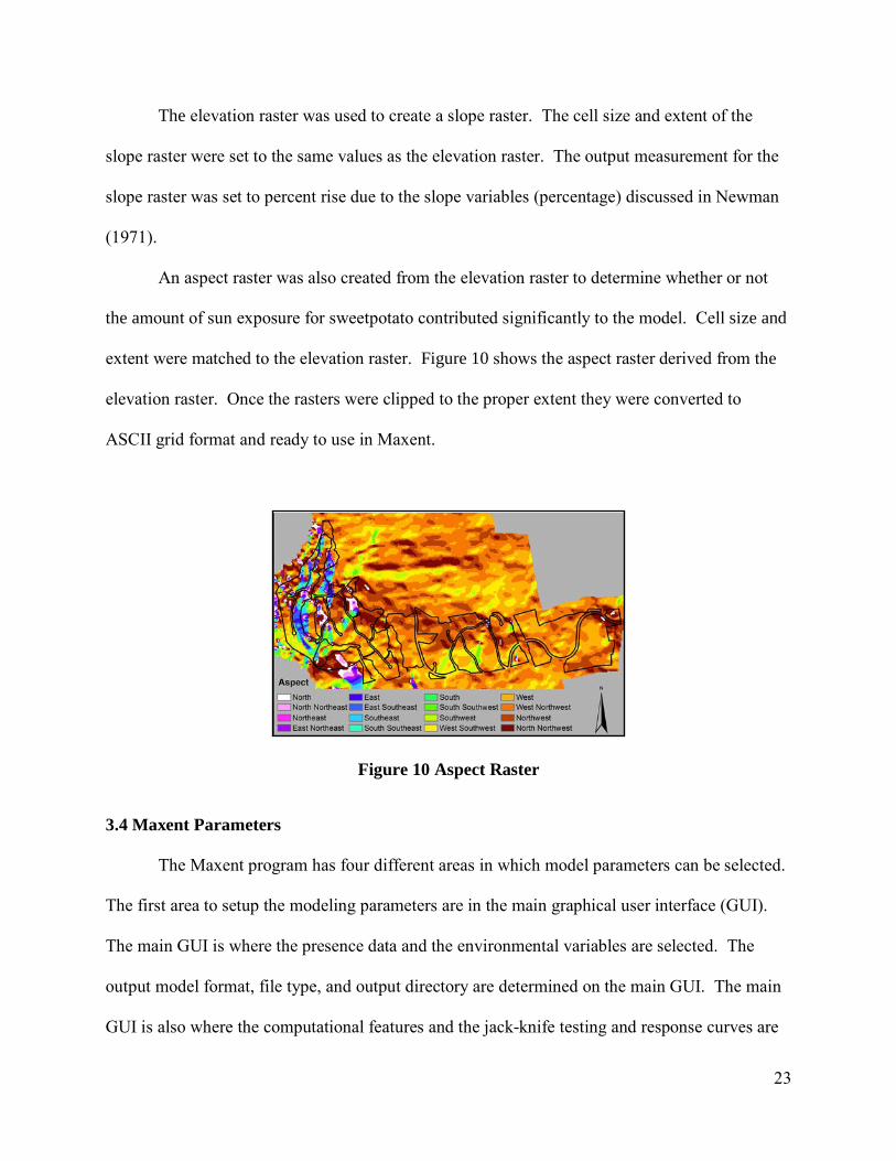
An aspect raster was also created from the elevation raster to determine whether or not
the amount of sun exposure for sweetpotato contributed significantly to the model. Cell size and
extent were matched to the elevation raster. Figure 10 shows the aspect raster derived from the
elevation raster. Once the rasters were clipped to the proper extent they were converted to
ASCII grid format and ready to use in Maxent.
Figure 10 Aspect Raster
3.4 Maxent Parameters
The Maxent program has four different areas in which model parameters can be selected.
The first area to setup the modeling parameters are in the main graphical user interface (GUI).
The main GUI is where the presence data and the environmental variables are selected. The
output model format, file type, and output directory are determined on the main GUI. The main
GUI is also where the computational features and the jack-knife testing and response curves are

24
selected. The 'Settings' button is also on the main GUI and contains three tabs of parameters that
can be set for each model run. This section first discusses the parameters set on the main GUI
and then discusses the tabs in Settings.
3.4.1 Computational Features
Phillips, Dudík, and Schapire (2011), Merow, Smith and Silander (2013), and Elith et al.
(2011) provide descriptions of the computational feature types (Table 3) and explain the
appropriate use for each feature type. The computational features are used to constrain the
Maxent output based on the environmental variable values (Phillips, Dudík, and Schapire 2011).
Linear features constrain the output model to the same values for each continuous environmental
variable as the observed locations for that species. Quadratic features constrain the output model
to the same environmental variable variance as the presence-only data. Product features
constrain the covariance of one variable with other environmental variables by multiplying two
of the environmental variables. Threshold features create a probability grid where the
environmental variable value is greater than a threshold value. Hinge features also create a
probability grid for values above a threshold, but use a linear function to create a smoother
model. Discrete features are automatically created for each variable that is categorical rather
than continuous.
Maxent allows users to choose which type of calculation features to use based on how the
model should respond to the environmental variables. The number of presence samples
determines which features are used by default. Linear features are automatically chosen when
the sample number is below 10, Maxent automatically adds quadratic features when there are
more than 10 samples, hinge features are added when there are more than 15 samples, and
threshold and product features are added when there are more than 80 samples. Elith et al. (2011)
25
recommend simplifying Maxent models by using only hinge features to create an easily
interpreted model. It is hard to determine the nature of environmental variable interaction with a
small number of presence samples (Elith et al. 2011). Hinge features, like linear features are
based on a single environmental variable, but their values are a constant below a threshold value.
Hinge features are a special case of linear and threshold features and using them in the model
makes using linear and threshold features redundant (Elith et al. 2011; Merow, Smith, and
Silander 2013). Therefore, hinge, quadratic, and product features were utilized in the final model
of this project in order to create a distribution that showed the probability of where agricultural
clearing features may be present dependent upon the relationship and interaction of the
environmental variables.
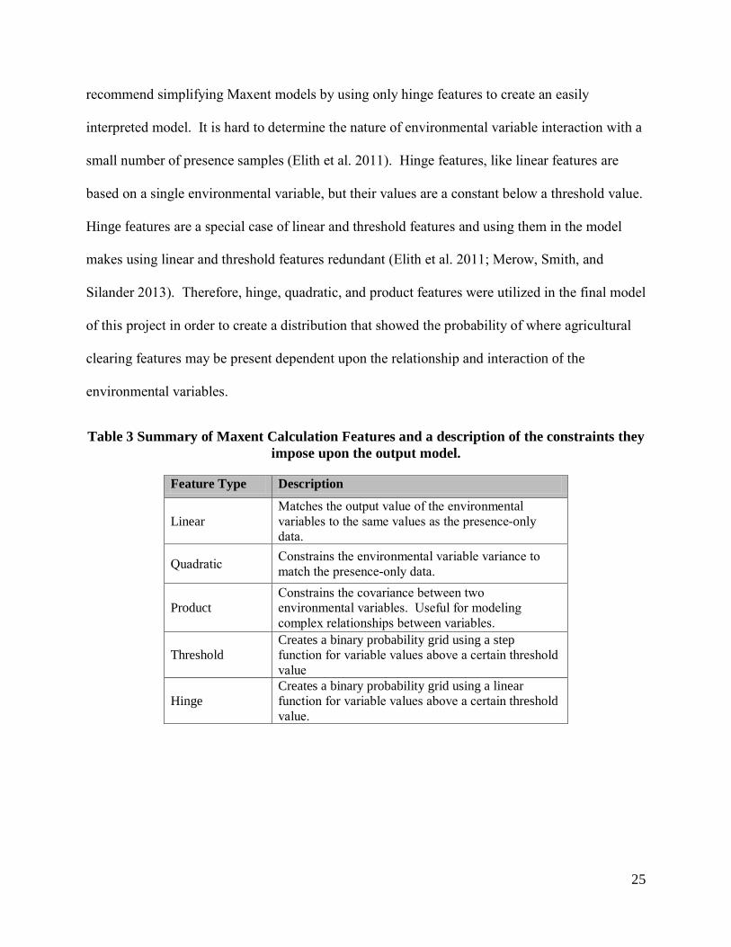
Table 3 Summary of Maxent Calculation Features and a description of the constraints they impose upon the output model.
Feature Type Description
Linear Matches the output value of the environmental variables to the same values as the presence-only data.
Quadratic Constrains the environmental variable variance to match the presence-only data.
Product Constrains the covariance between two environmental variables. Useful for modeling complex relationships between variables.
Threshold Creates a binary probability grid using a step function for variable values above a certain threshold value
Hinge Creates a binary probability grid using a linear function for variable values above a certain threshold value.
26
3.4.2 Environmental Variable Assessment in Maxent
The main Maxent GUI provides two options for assessing the importance of the
environmental variables to the model: (1) response curves and (2) jack-knife testing. Response
curves demonstrate the influence each environmental variable has on the Maxent model
(Phillips, Dudík, and Schapire 2011). Jack-knife testing creates models first omitting each
variable and then using only one variable to determine the importance of an environmental
variable to the predictive distribution of a species (Phillips, Dudík, and Schapire 2011). Both of
these options were selected to determine the importance of the environmental variables and to
observe whether or not the predictive distribution responded to each variable as expected.
3.4.3 Maxent Output Format
Maxent has three different output formats (1) raw, (2) logistic (default), and (3)
cumulative. The raw output shows a relative occurrence rate (ROR) of the target species
(Merow, Smith, and Silander 2013). The logistic output is a post processing of the raw output
and is used to show an approximate probability that the species will occur within a specific grid
cell (Phillips, Dudík, and Schapire 2011; Merow, Smith, and Silander 2013). The cumulative
output shows the suitability of conditions at a given location (Phillips, Dudík, and Schapire
2011). The logistic output format was chosen for this project because of its ease of interpretation
for species' probability of presence.
3.4.4 Maxent Settings
The Maxent settings GUI contains three different tabs, (1) Basic, (2) Advanced, and (3)
Experimental, where parameters are set before running Maxent. There are a total of 46
parameters among the three tabs. The parameters which can be set in Maxent are summarized in
Table 4.

27
Table 4 Modeling Parameters. These parameters affect the final output model produced by Maxent.
Parameter Tab Description Random seed Basic Random sets of sample points are used during each model run for
testing and training the model Random test percentage
Basic Percentage of presence samples set aside as test points used in evaluating the model
Regularization multiplier
Basic Multiply the regularization parameters by this number. The lower the number the tighter the distribution is to the presence-only data occurrences. A higher number creates a more diffuse distribution
Max number of background points
Basic The number of cells chosen at random for background points if the number of grid cells is larger than specified number
Replicates Basic Number of times to run the model.
Replicated run type Basic Testing and training method to use when running more than one replicate. Three types Cross Validation (divides samples into groups and each group takes a turn being used as test samples), Bootstrap (test samples chosen randomly by sampling with replacement), and Subsampling (test samples chosen randomly by sampling without replacement).
Maximum iterations
Advanced The maximum number of iterations to run before model learning is terminated.
Adjust sample radius
Advanced Adjust the size of the sample dots on the pictures of predictions by adding the specified number of pixels. Negative values reduce the size of the radius
Default prevalence Advanced Probability that an individual is observed at a suitable location Threads Experiment-
al Number of processor threads in a computer's central processing unit (CPU) to use.
Test runs were conducted using different parameter settings, environmental variables, and
presence point data in order to determine the parameter settings, environmental variables, and
agricultural feature types that would be used in the final model. More than 30 different test runs
were conducted and evaluated based on their goodness-of-fit, stability, environmental variable
performance, and whether or not the final model met expectations. Models for agricultural
clearing features, grow pits, and terraces were created. The paucity of presence data and
environmental variables for the grow pits and terraces created unreliable models. The abundance
of clearing feature presences (n=3743) appeared to compensate for the small number of

28
environmental variables and appeared to create reliable probability distributions which are
discussed in the next chapter. The parameters used in the final model are summarized in
Table 5.
Table 5 Final Model Parameters. These are the values, and the justification for those values, that the model parameters were set to during the final model run.
Parameter Value Justification Random seed True Random seeds are used to keep the bootstrapping runs from using
replicate test and training samples.
Random test percentage
25 Each model replicate used 25 percent of the samples for testing, training and statistics calculation
Regularization multiplier
8 Model runs indicated that this number was sufficiently large enough to create smooth response curves and spread-out the probability distribution from the presence-only data while maintaining a stable model.
Max number of background points
10000 Background points are used as pseudo-absences for model training. Presence probability is assumed to be unknown for each background point. The higher the number, the better the fit of the model. This number balanced speed and accuracy for modeling.
Replicates 100 Number of replicates sufficient enough to converge the average and median values of the Maxent output.
Replicated run type Bootstrap Bootstrapping created the models with the best goodness of fit and stability. Each of the 100 replicates run was able to use 25 percent of the sample points selected at random.
Maximum iterations
1000 The higher the number the more training that Maxent can do per replicate run resulting in a more stable model.
Adjust sample radius
0 Not pertinent to the final output of this model.
Default prevalence 0.8 Probability that an individual is observed at a suitable location
Threads 8 CPU used for the model runs was an Intel Core i7 I7-4770 3.4 GHz Quad-Core Processor. It has eight threads.

29
3.4.5 Model Validation
Maxent contains statistical tools to help in the validation of the output predictive
distributions. The main tool used to assess the goodness of fit for a Maxent model is the area
under the curve (AUC) which is determined by the receiver operating curve (ROC). The ROC,
in the case of Maxent, is a measure of the relative occurrence rate (ROR) because the model is
created using presence-only data (Merow, Smith, and Silander 2013). The response curves and
results from the jack-knife testing are additional tools created by Maxent to assess its outputs.
The final method of model validation, to be conducted in the future, will be ground truthing the
areas of dense vegetation.

30
CHAPTER 4: RESULTS
A prehistoric agricultural clearing feature probability distribution was produced using presence
point data and environmental variable raster data in the Maxent program. The output distribution
was produced as an ASCII grid. Maxent provides diagnostic tools that were used to assess the
reliability of the model. These tools include jack-knife testing to determine environmental
variable importance, response curves to demonstrate how the model responded to the
environmental variables, and area under the receiver operator curve (AUC) to assess the
goodness-of-fit of the model.
This chapter begins with a discussion of the output model generated by Maxent followed
by a discussion of model validity using the diagnostic tools available in Maxent.
4.1 Maxent Probability Distribution
The Maxent program uses a machine learning algorithm that trains itself by contrasting a
specified number of the available presence samples to a specified number of background sample
points. The background sample points are used as "pseudo absences" and the values are
contrasted with the values of the presence data. The final probability distribution here is a
product of 100 bootstrap replicate runs. Each run used 75 percent of the presence samples (n =
2808) and 10,000 background samples to train each model and 25 percent of the presence
samples (n = 935) to test each replicate model.
A smoothing filter was used in ArcMap 10.2.2 on the final output to smooth out the
values and create a more realistic model. The smoothing filter is a 9 cell (3x3) window that
passes over each cell in the raster dataset and assigns the average values of the 9 cells to the
center cell, reducing anomalies in the model. The higher values of the raster were reduced
slightly (95 to 92), but not enough to affect the overall predicted distribution of the agricultural

31
clearing features. Table 6 summarizes the change between the smoothed and unsmoothed raster.
The only value that changed is the max value.
Table 6 Minimum, maximum, and mean values of the unaltered output model and the smoothed output model.
Model Output Minimum Value Maximum Value Mean Value Unaltered Model 0 95 51 Smoothed Model 0 92 51
Figure 11 shows the final, smoothed average of the probability distributions of the 100
replicate runs, and the standard deviation of those runs. The values for the distribution are the
probability that the agricultural clearing features are present in each grid cell using breaks of 10
percent. The standard deviation is depicted using one percent breaks in order to better show the
variation in the standard deviation which ranges from close to zero to approximately 10.3 percent
and has the greatest values near the westernmost and at the easternmost extent of the model.
The modeled area extends the probability distribution of agricultural clearing features
beyond the boundaries of the AOI. Soil data variables were too homogenous and constrained the
model too tightly to the soil polygons, as a result, the soil data were not used in this model.
Elevation-derived data and rainfall datasets were used to create a more generalized model that
extends beyond the boundary of the AOI. The next section of this chapter discusses the
environmental variables and their performance in the model.
4.2 Environmental Variable Performance
Maxent creates a hypertext markup language (html) file that summarizes the model
results. It creates a file for each replicate model run and one file for the summary of all the
replicates. The results for the different diagnostic tests conducted by Maxent are included in
each of the html files. The environmental variable performance is evaluated using response
curves, contribution and permutation importance, and jack-knife testing.

32
Figure 11 Final Maxent output

33
4.2.1 Response Curves
Maxent creates two sets of response curves for the environmental variables. The first set
of curves are called marginal curves and they demonstrate how the model prediction changes as
the values of each environmental variable changes slightly while the rest of the variables remain
at their average values. Phillips, Dudík, and Schapire (2011) warn that the marginal curves may
be difficult to interpret if the environmental variables are correlated. The annual precipitation
(rf_ann) and summer precipitation (rf_summer) are highly correlated with the monthly rain
datasets; the values for annual and summer precipitation cannot be changed without changing the
values of the monthly precipitation datasets. As a result, The marginal response curves for this
model are not appropriate for determining how the Maxent output is affected by each
environmental variable.
The second set of response curves shows that the Maxent prediction reaches a peak and
then decreases as the values go up for each environmental variable. Figure 12 shows the
response curves created to represent a Maxent prediction that uses only that environmental
variable. The Y-axis for each of the response curves is the probability of agricultural feature
presence. The X-axis for the elevation response curve (elev) is elevation in feet, and the X-axis
for the rainfall response curves is rainfall in millimeters. The standard deviation for the 100
replicate runs, depicted in blue, increases as the number of presence samples represented for
those values of the environmental variables decrease.
Figure 12 shows the result of the "Identify" tool used in ArcMap 10.2.2. This tool has
been configured to show the cell values for each of the visible layers. The two results displayed
in Figure 10 show the values of the Maxent model, Agricultural Clearing Feature Average, along
with the values of the eight environmental variables that intersect with that Maxent model pixel.

34
Figure 12 Maxent output response curves.
Figure 13 Sample 'Identify' results for a Maxent model pixel with a low probability value (left) and a high probability value (right). Note that the variable values in the high probability
pixel are near to the peak values for each variable, while the reverse is true for the low probability pixel.

35
4.2.2 Environmental Variable Contribution and Importance to the Maxent Model
Maxent uses two different methods to estimate variable importance. The first method
implemented by Maxent creates a table using data gathered during the training of the model that
summarizes the environmental variable contribution to the model and the permutation
importance, or stability, of the variable. Variable contribution is determined by the amount of
increase or decrease of the model fit, called gain, caused by an environmental variable for each
iteration of the Maxent algorithm. The permutation importance is calculated by randomly
changing the value of an environmental variable among the model training points. The lower
this value is the more stable the variable's contribution to the model. The value of the decrease
in the training AUC is normalized so that the data can be represented as percentages for both the
percent contribution and the permutation importance (Phillips n.d.). Table 7 lists the
environmental variables used in this model and ranks them according to their contribution to the
model.
Table 7 Summary of Environmental Variables and Their Importance. The variables are ranked according to their percent contribution with September Rainfall having the most
contribution and July Rainfall the least contribution.
Variable Percent contribution
Permutation importance
September Rainfall 48.8 19.9 Elevation 22.5 17.9 Summer Rainfall 19.4 17.8 August Rainfall 5 24.6 June Rainfall 1.5 13.7 Slope 1.1 0.7 Annual Rainfall 1.1 0.8 July Rainfall 0.6 4.6

36
Another method that Maxent uses to determine variable importance is the jack-knife test.
The jack-knife test trains the model removing each environmental variable to calculate which
variable causes the largest decrease in the model's gain. This variable contains the most
information not found in the other environmental variables. The second part of the jack-knife
test is training the model using each environmental variable by itself. The environmental
variable with the highest gain is considered to have the most useful information by itself. The
summer rainfall variable (rf_summer) caused the largest decrease in the gain averaged over the
100 replicate runs of this model. The September rainfall variable (rf_sep) had the highest gain
when used alone for training. The Maxent output, however, warns that caution must be used
when interpreting the results of jack-knife testing when the environmental variables are highly
correlated, as the rainfall variables are in this case.
4.3 Model Performance
The area under the receiver operator curve (AUC) is the most commonly used diagnostic
to evaluate a Maxent model (Merow, Smith, and Silander 2013). The AUC is a comparison of
the true positive rate and the false positive rate, or how well the model is able to predict presence
and absence. Maxent uses presence-only data. The AUC created for Maxent models shows how
well the model is able to distinguish presence from random (Phillips, Anderson, and Schapire
2005). The value for the AUC ranges from 0 to 1, the closer the value of the AUC is to 1 the
better the fit of the model. An AUC value of 0.5 equals random prediction (Phillips, Anderson,
and Schapire 2005). The average AUC for the 100 replicates of this model was 0.819 with a
standard deviation of 0.009.
According to the diagnostic tools provided by Maxent, the model produced for this
project performs well. The next chapter discusses the results of the model with respect to the

37
expectations presented by the conceptual model in Chapter 2. Chapter 5 also discusses the
applicability of Maxent in archaeology, future work, and improvements that can be made to the
current model.

38
CHAPTER 5: DISCUSSION AND CONCLUSIONS
The purpose of this thesis was to assess the usefulness of Maxent for predicting the presence of
archaeological features. A recent archaeological survey of agricultural features within a portion
of the Hōkūli‘a luxury development on Hawai‘i Island provided the opportunity to test Maxent
(See Figure 1 in Chapter 1). This chapter discusses the results of the Maxent model, how they
compare to the conceptual model and expectations of agricultural feature distribution in the Kona
Field System, how human behavior may affect the interpretation of the results, limitations of this
model, and the usefulness and applicability of using Maxent in an archaeological context.
5.1 Model Evaluation
The diagnostic tools included as part of the Maxent package indicated that the model
produced for this project is a strong, reliable model. Three research hypotheses listed in Chapter
1 were also used to evaluate the model. The first hypothesis states that agricultural clearing
feature density increases with elevation from the shoreline to the upper elevations of the kula
zone and the lower elevations of the kaluulu zone (approximately 0—680 ft elevation), and that
the feature density should start to decrease starting in the middle elevations of the kaluulu zone
(approximately 680 ft elevation). This distribution pattern was noted during an archaeological
inventory survey conducted three kilometers to the north of the current AOI by Haun and Henry
(2010).
The model shows that the region within the AOI that has the highest probability of
agricultural clearing features ranges in elevation from approximately 175 ft to 600 ft. Figure 14
shows the modeled probability distribution overlaid with elevation contours to illustrate this.
Cells within the elevation range of 175 ft—600 ft have an 80 percent or better probability of
containing an agricultural clearing feature. Figure 15 shows the response curve for an elevation-

39
only model created within Maxent. The response curve shows that there is a 70 percent or better
probability of agricultural clearing features present in the 50 ft—680 ft elevation range.
The results for the distribution of agricultural features with respect to elevation do not
exactly match the observations made by Haun and Henry (2010), but that does not invalidate the
model. The model does show a general trend of increasing presence with elevation before
peaking and presence probability starts to decline above 350 ft in elevation. This apparent lack
of correspondence may be due to the fact that elevation is not the only variable involved in this
model.
The second hypothesis states that as precipitation levels approach acceptable levels for
dryland taro farming, there is a decrease in the density of informal clearing features that are used
in sweetpotato cultivation. As noted in Chapter 2, Valenzuela, Fukuda, and Arakaki (2000)
Figure 14 Agricultural Clearing Feature Probability Distribution With Elevation Overlay

40
Figure 15 Elevation Response Curve Showing the Average Values and Standard Deviation from the 100 Maxent Replicate Models
identify the rainfall tolerance for sweetpotato to be 500—1300 mm per growth cycle and the
optimal rainfall to be 900—1300 mm. Ladefoged et al (2009) used 750—1000 mm as their
optimal range for sweetpotato cultivation. Handy, Handy, and Pukui (1991) identified the
rainfall during the summer months as the most important for sweetpotato cultivation in the Kona
Field System.
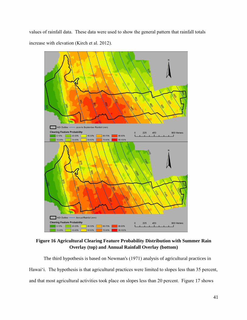
Figure 16 shows the output model with an overlay of the summer months' rainfall as well
as the output model with annual rainfall. The figure shows that there is a good probability for
agricultural clearing feature presence between 340 mm—460 mm of summer rain, which
correlates to approximately 810 mm—1,050 mm of annual rainfall (See Figure 16). The highest
probability of feature presence (greater than 80 percent) does occur within the annual rainfall
range of 850 mm—990 mm. This is relatively close to the range used by Ladefoged et al (2009).
The rainfall data used in this model is modern and attention should not be focused on the actual
41
values of rainfall data. These data were used to show the general pattern that rainfall totals
increase with elevation (Kirch et al. 2012).
Figure 16 Agricultural Clearing Feature Probability Distribution with Summer Rain Overlay (top) and Annual Rainfall Overlay (bottom)
The third hypothesis is based on Newman's (1971) analysis of agricultural practices in
Hawai‘i. The hypothesis is that agricultural practices were limited to slopes less than 35 percent,
and that most agricultural activities took place on slopes less than 20 percent. Figure 17 shows

42
the response curve for the average of 100 models using only the slope variable within Maxent.
The X-axis values for the graph are percent slope. The response curve shows that the probability
of presence for agricultural clearing features peaks at approximately 30 percent slope and
decreases as the percent slope value rises above 30 percent. This number does not quite match
Newman's (1971) observation but it does show that agricultural activity declines above a certain
slope.
The Maxent probability distribution model shows that the greatest concentration of
agricultural clearing features occurs within the kula zone and lower kaluulu zone. This is an
ecological model that uses environmental variables to determine the probability that a cell within
the model surface will contain an individual of the species of interest, agricultural clearing
features in this case. Importantly, however, the model does not take into account human
behavior and cultural factors so it is important to consider the human role on the distribution of
agricultural practices.
Figure 17 Elevation Response Curve of Clearing Feature Probability to Slope Variable

43
The environmental variables determine, to an extent, how and where crops can be
cultivated. People are capable of altering the landscape to increase the cultivability of an area
and to grow crops in relatively marginal areas (Kirch et al. 2004; Vitousek et al. 2004). Vitousek
et al. (2004) did observe areas in Hawai‘i suitable for dryland agriculture that were not cultivated
demonstrating that even though an area was suitable for farming, there is the possibility that it
was not cultivated. Historical and cultural factors help in understanding human behavior and
cultural development (Freilich 1967). Human behavior must be kept in mind when interpreting
this model.
The areas modeled as low probability of agricultural clearing feature presence may be an
underestimation of the features that may be present. Native Hawaiians developed farming
techniques to address the challenges posed by different regions (Handy, Handy, and Pukui 1991).
Kirch et al. (2004) noted that Native Hawaiians, at times, were forced to farm in marginal areas
to feed growing populations. The actual presence of agricultural clearing features could be
greater than predicted by the ecological model due to this behavior.
On the other hand, areas that are suitable for agricultural cultivation may be important for
spiritual or cultural reasons that are not obvious. Spiritual and cultural importance may be
intangible and cannot be measured or evaluated empirically (King 2003). This may cause
agriculturally suitable areas to remain uncultivated, in which case the model may overestimate
the probability of agricultural clearing feature presence. For example, Pu‘u Ohau, a culturally
significant cinder cone, is located in the southwest corner of the model and may be an area where
the probability of agricultural clearing feature presence may be overestimated. The model
calculates that the eastern slope of the pu‘u has a high probability of agricultural clearing feature
presence. However, Pu‘u Ohau contains a number of burial and ceremonial sites (Kaschko 1984;

44
Hammatt et al. 1997; Belt Collins Hawaii 2007) and this Maxent model cannot not account for
these sites and the spiritual and cultural importance of Pu‘u Ohau.
5.1.1 Archaeological Monitoring and Future Model Evaluation
In the future, model performance will be evaluated in the field as a by-product of
archaeological monitoring of ground disturbing activities to be conducted within the AOI. The
archaeological monitor will be required to record any features that are encountered during these
activities (Tomonari-Tuggle and Tuggle 1999) and the data collected will be used to evaluate the
Maxent model. Of course, it will not be possible to evaluate through ground truthing the model
performance for the areas that have been completely altered by heavy machinery (e.g. the golf
course) as there is no evidence left of the cultural resources that were present within those areas.
5.2 Conclusions
The probability distribution of agricultural clearing features modeled by the Maxent
program appears to be a reliable and stable model based on the diagnostic tests conducted within
Maxent. The mean AUC for the 100 replicates is 0.819 with a standard deviation of 0.009 which
is an indicator that the model performs well, the closer the AUC is to 1.0 the better the model
performance (Phillips n.d.). The environmental variable response curves show the model
responding to individual variables as predicted by the conceptual model.
This model could be improved with a better elevation dataset. The elevation data used in
this model included recent alterations to the landscape such as house lot grades, the golf course,
manmade ponds, and roads. These landscape alterations may have affected the influence of the
slope variable on the probability distribution.
Maxent's usefulness in regards to modeling archaeological feature distribution is
conditional and is dependent upon the number of presence samples that are used to create the

45
model. Test models were produced while the archaeological agricultural feature survey, which
provided the presence data for this project, was in progress. Variable contributions and
importance changed with the number as well as the distribution of the presence samples.
Probability distributions for agricultural terraces and grow pits were also created using Maxent,
but the models produced for these feature types were unreliable and the results were not useful
due to the small number of presence samples used by the model.
As a result of this research, it is concluded that Maxent can be used to model prehistoric
agricultural systems by using environmental variables that can define the proper growing
conditions for the crops cultivated within that system. Maxent cannot model human behavior
and may overestimate feature presence in spiritually important areas that are suitable for crop
cultivation where farming does not occur. The variables that define the spiritual importance of a
place are often intangible and cannot be empirically recorded (King 2003). As a result, these
spiritual variables cannot be used in Maxent.
Despite this inability to model human behavior, this research suggests that there is further
use for Maxent in the Kona Field System. The program and technique offer a way to synthesize
the commercial archaeology data of the region to create a more complete picture of the Kona
Field System than the piecemeal study areas do on their own. Soil attribute data could also be
added back into the model over the larger geographic region as there is more than one soil type
present within the larger Kona Field System. The Maxent program should be able to reliably
model the distribution of agricultural features in kula and kaluulu zones as the majority of the
agricultural features present within those zones can be represented as points. However, the linear
mounds and long, cross-slope terraces observed in the formal areas of the Kona Field System,
the ‘āpa‘a zone, present a challenge for Maxent since they are linear features rather than points.

46
This could be resolved by using coarser environmental data at a smaller scale and placing points
in the center of the agricultural fields for the presence data as done by Kemp (2012). Using
Maxent to model the Kona Field System may expand its extent beyond the currently accepted
boundaries.
While Maxent is incapable of reliably modeling human habitation sties, burials, and
ceremonial sites it can model regions of human activities that are partially dependent upon
environmental variables. Modeling the distribution of these activities, e.g. farming, can be used
as a proxy in trying to determine areas that may be of cultural importance. Haun and Henry
(2010) showed that there were large habitation complexes and substantial ceremonial sites
located within areas that were densely covered by agricultural features. The Maxent model can
be used to determine which areas warrant further archaeological investigation and provide an
idea of the level of effort that an area may require to be properly documented.
47
References
Allen, Melinda S. 2004. "Bet-Hedging Strategies, Agricultural Change, and Unpredictable
Environments: Historical Development of Dryland Agriculture in Kona, Hawaii." Journal of
Anthropological Archaeology 23 (2): 196-224.
doi:http://dx.doi.org.libproxy.usc.edu/10.1016/j.jaa.2004.02.001.
———. 2001a. "Cultural Setting and Recent Garden History." In Gardens of Lono:
Archaeological Investigations at the Amy B.H. Greenwell Ethnobotanical Garden
Kealakekua, Hawai'i, edited by Melinda S. Allen, 1-13. Honolulu, Hawai'i: Bishop Museum
Press.
———. 2001b. "The Environmental Context of Traditional Dryland Agriculture in Kona." In
Gardens of Lono: Archaeological Investigations at the Amy B.H. Greenwell Ethnobotanical
Garden Kealakekua, Hawai'i, edited by Melinda S. Allen, 15-22. Honolulu, Hawai'i: Bishop
Museum Press.
Anderson, Robert P., Daniel Lew, and A. Townsend Peterson. 2003. "Evaluating Predictive
Models of Species’ Distributions: Criteria for Selecting Optimal Models." Ecological
Modelling 162 (3): 211-232. doi:http://dx.doi.org.libproxy.usc.edu/10.1016/S0304-
3800(02)00349-6.
Arnese, Alessio. 2008. "Applying Ecological Niche Factor Analysis for Predictive Modelling in
the Kaulonia Field Survey. Layers of Perception. Proceedings of the 35th International
Conference on Computer Applications and Quantitative Methods in Archaeology
(CAA). Axel, P, K. Lambers, and I. Herzog Editors.<br /><br />." Berlin Germany, April 2-
6, 2007.

48
Belt Collins Hawaii, Ltd. 2007. Supplemental Environmental Impact Statement Preparation
Notice, Hokuli`a, North Kona and South Kona Island of Hawai`i. Hawaii.
Cordy, Ross. 2000. Exalted Sits the Chief: The Ancient History of Hawai`i Island. Honolulu, HI:
Mutual Publishing.
Elith, Jane, Steven J. Phillips, Trevor Hastie, Miroslav Dudík, Yung En Chee, and Colin J. Yates.
2011. "A Statistical Explanation of Maxent for Ecologists." Diversity and Distributions
(17): 43-57.
Ellis, William. 1917. A Narrative of a Tour through Hawaii, Or Owhyhee; with Remarks on the
History, Traditions, Manners, Customs and Language of the Inhabitants of the Sandwich
Islands. Honolulu, HI: Hawaiian Gazette Co., Ltd.
Esri. "Georeferencing a Raster Dataset." ArcGIS Desktop 9.3 Help. Esri, last modified
November 12, 2009, accessed March 14, 2015,
http://webhelp.esri.com/arcgisdesktop/9.3/index.cfm?TopicName=Georeferencing_a_raster
_dataset.
Freilich, Morris. 1967. "Ecology and Culture: Environmental Determinism and the Ecological
Approach in Anthropology." Anthropological Quarterly 40 (1): 26-43.
http://www.jstor.org.libproxy.usc.edu/stable/3316830.
Galletti, Christopher S., Elizabeth Ridder, Steven E. Falconer, and Patricia L. Fall. 2013.
"Maxent Modeling of Ancient and Modern Agricultural Terraces in the Troodos Foothills,
Cyprus." Applied Geography (39): 46-56.
Giambelluca, Thomas W., Qi Chen, Abby G. Frazier, Jonathan P. Price, Yi-Leng Chen, Pao-Shin
Chu, Jon K. Eischeid, and Donna M. Delparte. 2013. "Online Rainfall Atlas of Hawai‘i."

49
Bulletin of the American Meteorological Society 94: 313-316. doi:10.1175/BAMS-D-11-
00228.1.
Haegeman, Bart and Michel Loreau. 2008. "Limitations of Entropy Maximization in Ecology."
Oikos (117): 1700-1710.
Hammatt, Hallet H., Douglas F. Borthwick, Brian L. Colin, Ian Masterson, Jennifer J. Robins,
and Helen Wong-Smith. 1997. Archaeological Inventory Survey and Limited Subsurface
Testing of a 1,540-Acre Parcel in the Ahupua‘a of Honuaino, Hokukano, Kanaueue,
Haleki‘i, Ke‘eke‘e,‘Ilikahi, Kanakau, Kalukalu, and Onouli, Districts of North and South
Kona. Vol. I, II, and III. Kailua, Hawaii: Cultural Surveys Hawai‘i.
Handy, E. S. Craighill, Elizabeth Green Handy, and Mary Kawena Pukui. 1991. Native Planters
in Old Hawaii: Their Life, Lore, & Environment. Honolulu, HI: Bishop Museum Press.
Haun, Alan E. and J. David Henry. 2010. Archaeological Inventory Survey TMK: (3) 7-9-05:76,
77 and 78, Lands of Honalo, Ma‘ihi 1-2 and Kuamo‘o 1, North Kona District, Island of
Hawaii. Kailua Kona, Hawaii: Haun & Associates.
Hirzel, Alexandre H. and Gwenaëlle Le Lay. 2008. "Habitat Suitability Modelling and Niche
Theory." Journal of Applied Ecology (45): 1372-1381.
Jaynes, Edwin T. 1957. "Information Theory and Statistical Mechanics." Physical Review 106
(4): 620-630. doi:10.1103/PhysRev.106.620.
Kailihiwa, Solomon. "Hōkūli‘a Agricultural Feature Survey Data during Monitoring."
Archaeological Spatial and Attribute Data, Unpublished Data, .
Kaschko, Michael. 1984. Pu‘u Ehu Estates. Hilo, Hawaii: Paul H. Rosendahl, Ph.D., Inc.
Kelly, Marion. 1983. Nā Māla O Kona: Gardens of Kona, a History of Land use in Kona,
Hawai‘i. Honolulu, HI: Department of Anthropology Bernice P. Bishop Museum.
50
Kemp, Karen K. 2012. The Hawai`i Island Crop Probability Map: An Update of the Crop
Growth Parameters for the Hawai`i County Crop Model: Final Report Prepared for the
County of Hawai`i Research Adn Development Department.
King, Thomas F. 2003. Places that Count, Traditional Cultural Properties in Cultural Resource
Management. Heritage Resource Management Series., edited by Don Fowler. Lanham,
Maryland: AltaMira Press.
Kirch, P. V., G. Asner, O. A. Chadwick, J. Field, T. Ladefoged, C. Lee, C. Puleston, S.
Tuljapurkar, and P. M. Vitousek. 2012. "Building and Testing Models of Long-Term
Agricultural Intensification and Population Dynamics: A Case Study from the Leeward
Kohala Field System, Hawai’i." Ecological Modelling 227 (0): 18-28.
doi:http://dx.doi.org.libproxy.usc.edu/10.1016/j.ecolmodel.2011.11.032.
Kirch, P. V., A. S. Hartshorn, O. A. Chadwick, P. M. Vitousek, D. R. Sherrod, J. Coil, L. Holm,
and W. D. Sharp. 2004. "Environment, Agriculture, and Settlement Patterns in a Marginal
Polynesian Landscape." Proceedings of the National Academy of Sciences of the United
States of America 101 (26): 9936-9941. doi:10.1073/pnas.0403470101.
Ladefoged, Thegn N., Patrick Vinton Kirch, Samuel M. Gon III, Oliver A. Chadwick, Anthony
S. Hartshorn, and Peter M. Vitousek. 2009. "Opportunities and Constraints for Intensive
Agriculture in the Hawaiian Archipelago Prior to European Contact." Journal of
Archaeological Science 36: 2374-2383.
Ledyard, John. 1963. John Ledyard's Journal of Captain Cook's Last Voyage, edited by James
Kenneth Munford. Corvallis, OR: Oregon State University Press.

51
Lincoln, Noa and Thegn Ladefoged. 2014. "Agroecology of Pre-Contact Hawaiian Dryland
Farming: The Spatial Extent, Yield and Social Impact of Hawaiian Breadfruit Groves in
Kona, Hawai`i." Journal of Archaeological Science 49: 192-202.
Menzies, Archibald. 1920. Hawaii Nei 128 Years Ago, edited by William Frederick Wilson.
Honolulu, HI:.
Merow, Cory, Matthew J. Smith, and John A. Silander. 2013. "A Practical Guide to MaxEnt for
Modeling Species? Distributions: What it does, and Why Inputs and Settings Matter."
Ecography 36 (10): 1058-1069. doi:10.1111/j.1600-0587.2013.07872.x.
Newman, T. Stell. 1971. "Hawaii Island Agricultural Zones, Circa A. D. 1823: An
Ethnohistorical Study." Ethnohistory 18 (4): 335-351.
Pearson, Richard G., Christopher J. Raxworthy, Miguel Nakamura, and A. Townsend Peterson.
2007. "ORIGINAL ARTICLE: Predicting Species Distributions from Small Numbers of
Occurrence Records: A Test Case using Cryptic Geckos in Madagascar." Journal of
Biogeography 34 (1): 102-117. doi:10.1111/j.1365-2699.2006.01594.x.
Phillips, Steven J. "A Brief Tutorial on Maxent." Unpublished tutorial distributed with software.
Phillips, Steven J., Robert P. Anderson, and Robert E. Schapire. 2005. "Maximum Entropy
Modeling of Species Geographic Distributions." Ecological Modelling 190 (2006): 231-259.
Phillips, Steven J. and Miroslav Dudík. 2008. "Modeling of Species Distributions with Maxent:
New Extensions and a Comprehensive Evaluation." Ecography (31): 161-175.
Phillips, Steven J., Miroslav Dudík, and Robert E. Schapire. 2004. "A Maximum Entropy
Approach to Species Distribution Modeling." Proceedings of the Twenty-First International
Conference on Machine Learning: 655-662.
———. 2011. Maximum Entropy Modeling of Species Geographic Distribution. Vol. 3.3.3k.

52
Roxburgh, Stephen H. and Karel Mokany. 2010. "On Testing Predictions of Species Relative
Abundance from Maximum Entropy Optimisation." Oikos (119): 583-590.
Tomonari-Tuggle, Myra J. and H. David Tuggle. 2008. Hōkūli‘a Preservation Plan for Non-
Burial Sites at Hōkūli‘a, Districts of North and South Kona, Island of Hawai‘i (TMK 7-9-
12:4). Report Prepared for 1250 Oceanside Partners by International Archaeological
Research Institute, Inc.
———. 1999. Hokuli‘a: An Integrated Archaeological Mitigation Plan. Honolulu, Hawaii:
International Archaeological Research Institute, Inc.
Valenzuela, Hector, Steven Fukuda, and Alton Arakaki. 2000. Sweetpotato Production
Guidelines for Hawaii. Honolulu, Hawaii: Agricultural Publications Distribution Office,
College of Tropical Agriculture and Human Resources. University of Hawai'i at Manoa.
Vitousek, P. M., T. N. Ladefoged, P. V. Kirch, A. S. Hartshorn, M. W. Graves, S. C. Hotchkiss,
S. Tuljapurkar, and O. A. Chadwick. 2004. "Soils, Agriculture, and Society in Precontact
Hawai`i." Science 304 (5677): 1665-1669. doi:10.1126/science.1099619.
Recommended