
Bootstrapping Time Series Data
Paul TeetorQuant Development LLC
CSP 2015New Orleans, LA
2
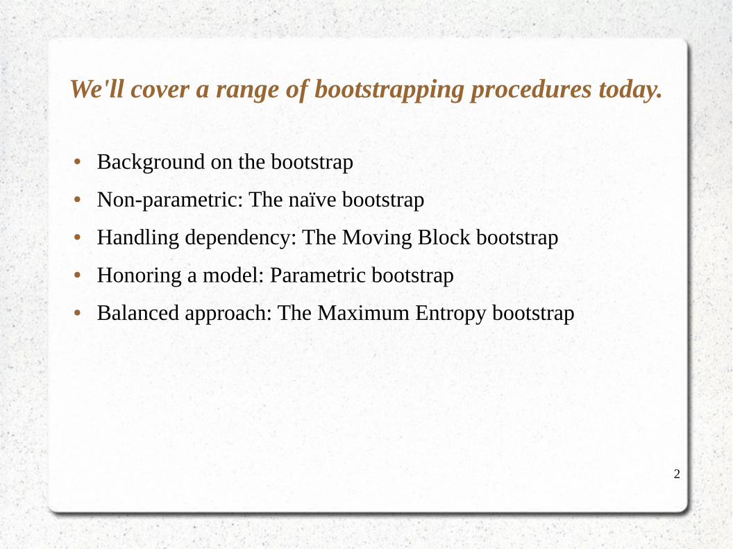
We'll cover a range of bootstrapping procedures today.
● Background on the bootstrap
● Non-parametric: The naïve bootstrap
● Handling dependency: The Moving Block bootstrap
● Honoring a model: Parametric bootstrap
● Balanced approach: The Maximum Entropy bootstrap
3
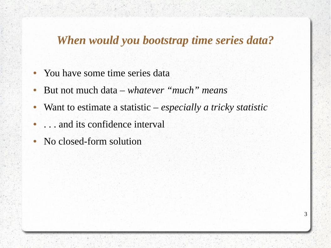
When would you bootstrap time series data?
● You have some time series data
● But not much data – whatever “much” means
● Want to estimate a statistic – especially a tricky statistic
● . . . and its confidence interval
● No closed-form solution
4
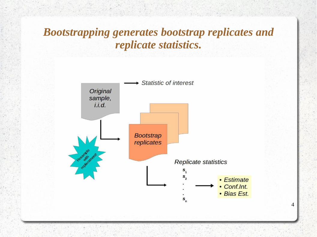
Bootstrapping generates bootstrap replicates and replicate statistics.
5
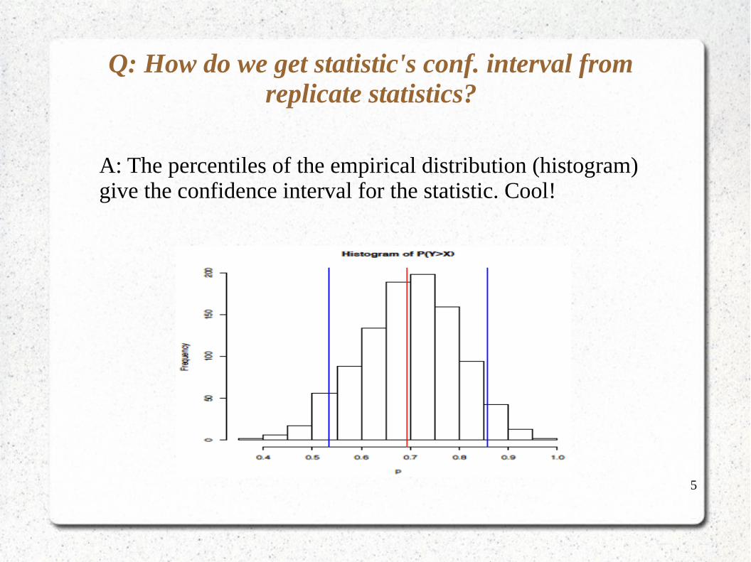
Q: How do we get statistic's conf. interval from replicate statistics?
A: The percentiles of the empirical distribution (histogram) give the confidence interval for the statistic. Cool!
6
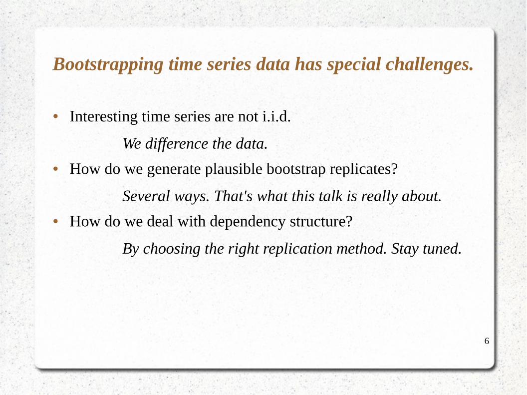
Bootstrapping time series data has special challenges.
● Interesting time series are not i.i.d.
We difference the data.
● How do we generate plausible bootstrap replicates?
Several ways. That's what this talk is really about.
● How do we deal with dependency structure?
By choosing the right replication method. Stay tuned.
7
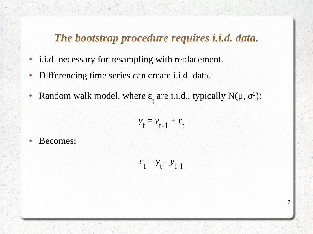
The bootstrap procedure requires i.i.d. data.
● i.i.d. necessary for resampling with replacement.
● Differencing time series can create i.i.d. data.
● Random walk model, where εt are i.i.d., typically N(μ, σ2):
yt = y
t-1 + ε
t
● Becomes:
εt = y
t - y
t-1
8
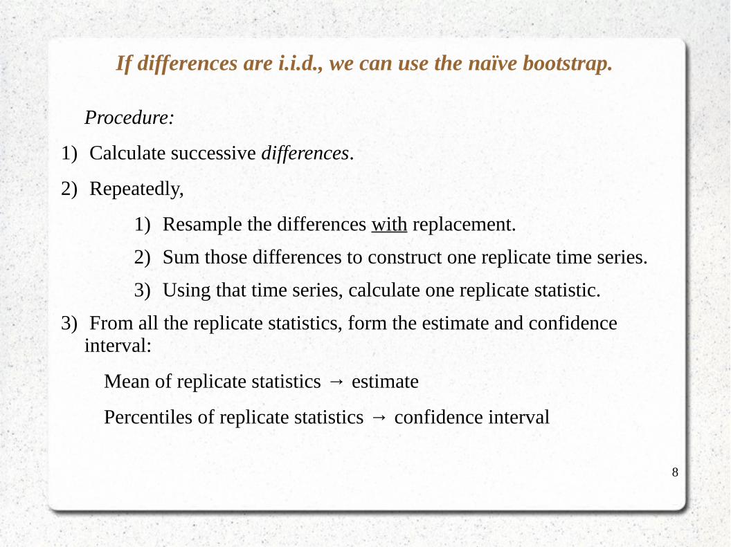
If differences are i.i.d., we can use the naïve bootstrap.
Procedure:
1) Calculate successive differences.
2) Repeatedly,
1) Resample the differences with replacement.
2) Sum those differences to construct one replicate time series.
3) Using that time series, calculate one replicate statistic.
3) From all the replicate statistics, form the estimate and confidence interval:
Mean of replicate statistics → estimate
Percentiles of replicate statistics → confidence interval
9
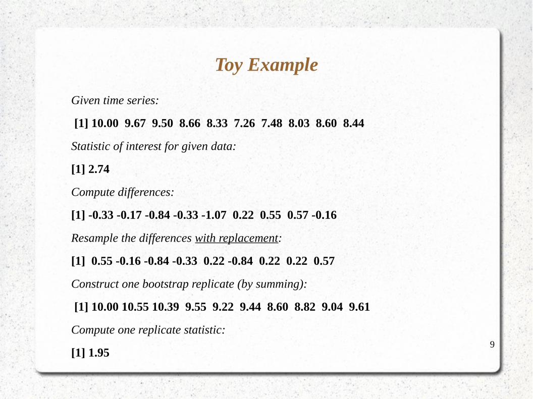
Toy Example
Given time series:
[1] 10.00 9.67 9.50 8.66 8.33 7.26 7.48 8.03 8.60 8.44
Statistic of interest for given data:
[1] 2.74
Compute differences:
[1] -0.33 -0.17 -0.84 -0.33 -1.07 0.22 0.55 0.57 -0.16
Resample the differences with replacement:
[1] 0.55 -0.16 -0.84 -0.33 0.22 -0.84 0.22 0.22 0.57
Construct one bootstrap replicate (by summing):
[1] 10.00 10.55 10.39 9.55 9.22 9.44 8.60 8.82 9.04 9.61
Compute one replicate statistic:
[1] 1.95
10
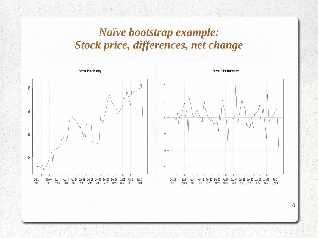
Naïve bootstrap example:Stock price, differences, net change
11
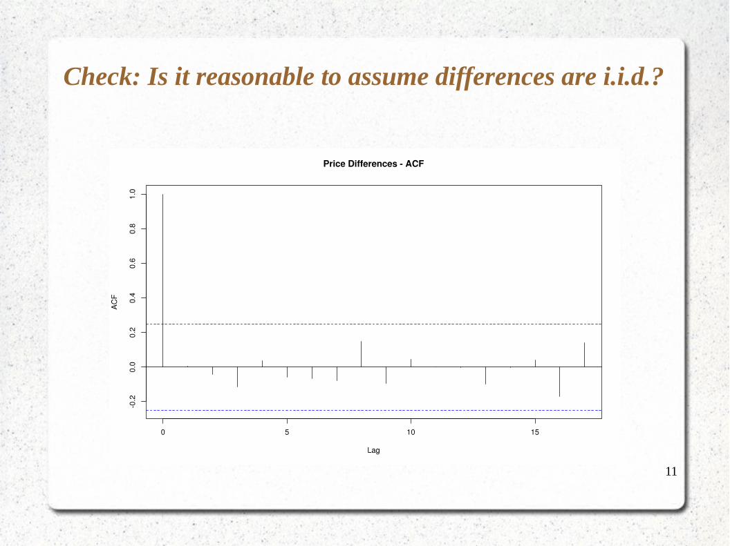
Check: Is it reasonable to assume differences are i.i.d.?
12
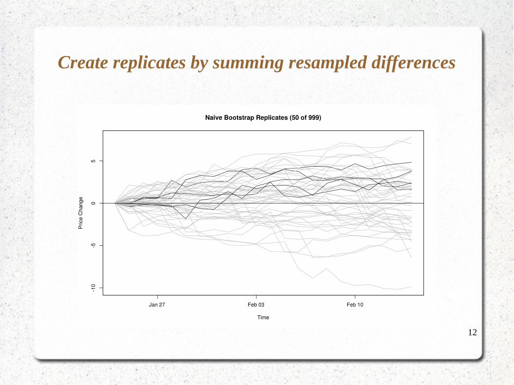
Create replicates by summing resampled differences
13
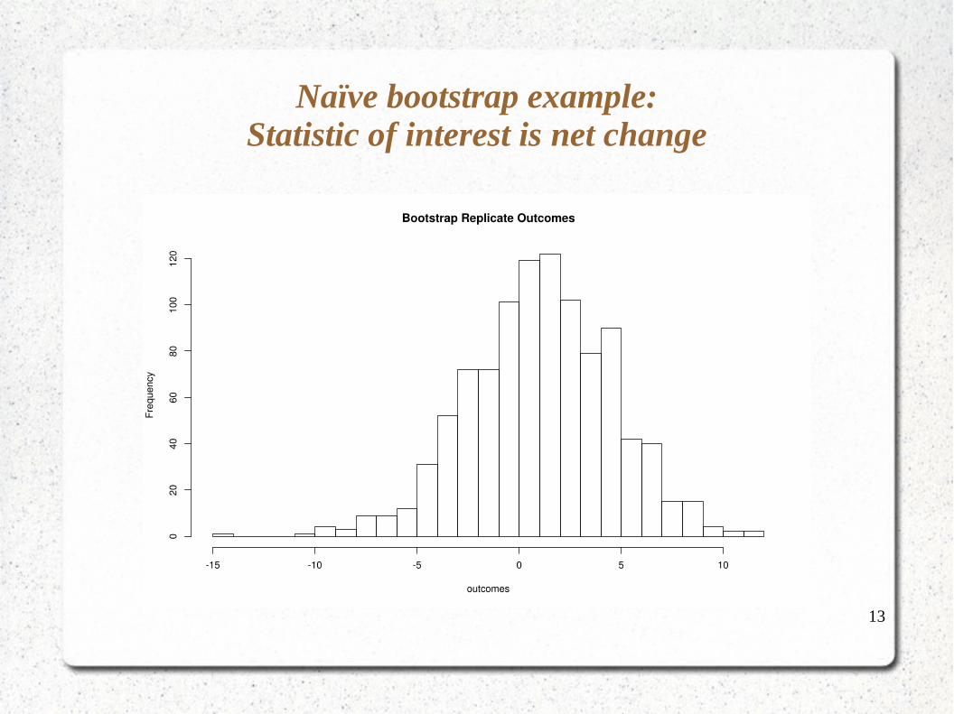
Naïve bootstrap example:Statistic of interest is net change
14
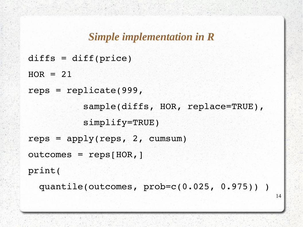
Simple implementation in R
diffs = diff(price)
HOR = 21
reps = replicate(999,
sample(diffs, HOR, replace=TRUE),
simplify=TRUE)
reps = apply(reps, 2, cumsum)
outcomes = reps[HOR,]
print(
quantile(outcomes, prob=c(0.025, 0.975)) )
15
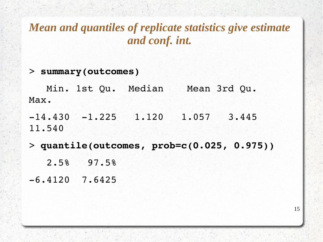
Mean and quantiles of replicate statistics give estimate and conf. int.
> summary(outcomes)
Min. 1st Qu. Median Mean 3rd Qu. Max.
14.430 1.225 1.120 1.057 3.445 11.540
> quantile(outcomes, prob=c(0.025, 0.975))
2.5% 97.5%
6.4120 7.6425
16
Next problem:What if the differences are not i.i.d.?
If not, purely random resampling will not capture the structure of the differences.
Bootstrap replicates will not resemble our data.
Uh oh.
17
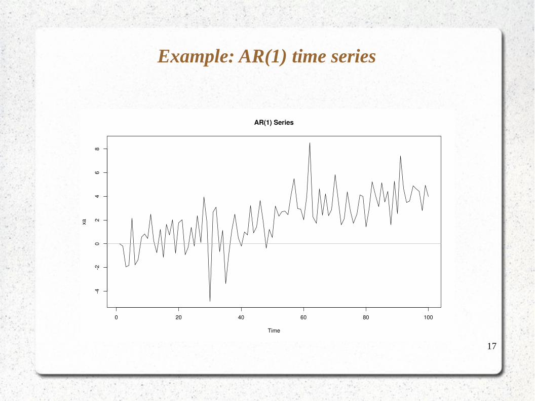
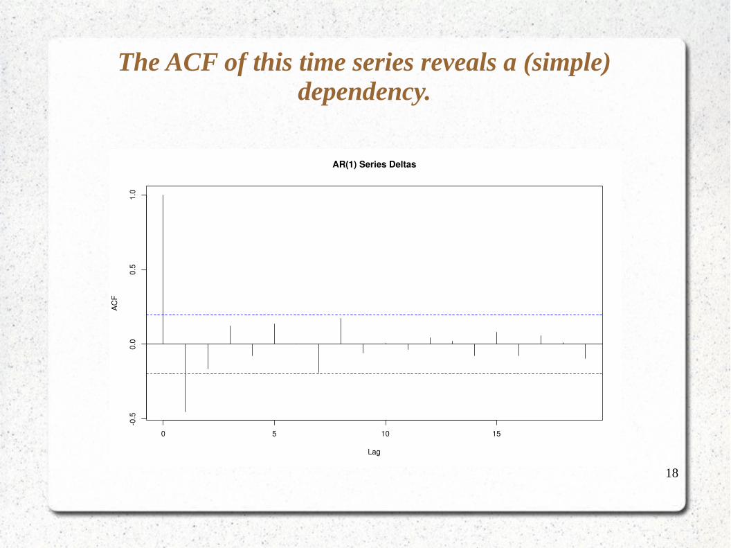
Example: AR(1) time series
18
The ACF of this time series reveals a (simple) dependency.
19
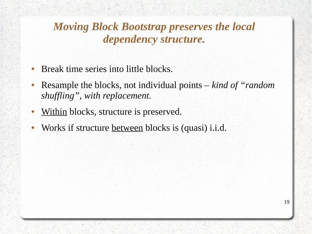
Moving Block Bootstrap preserves the local dependency structure.
● Break time series into little blocks.
● Resample the blocks, not individual points – kind of “random shuffling”, with replacement.
● Within blocks, structure is preserved.
● Works if structure between blocks is (quasi) i.i.d.
20
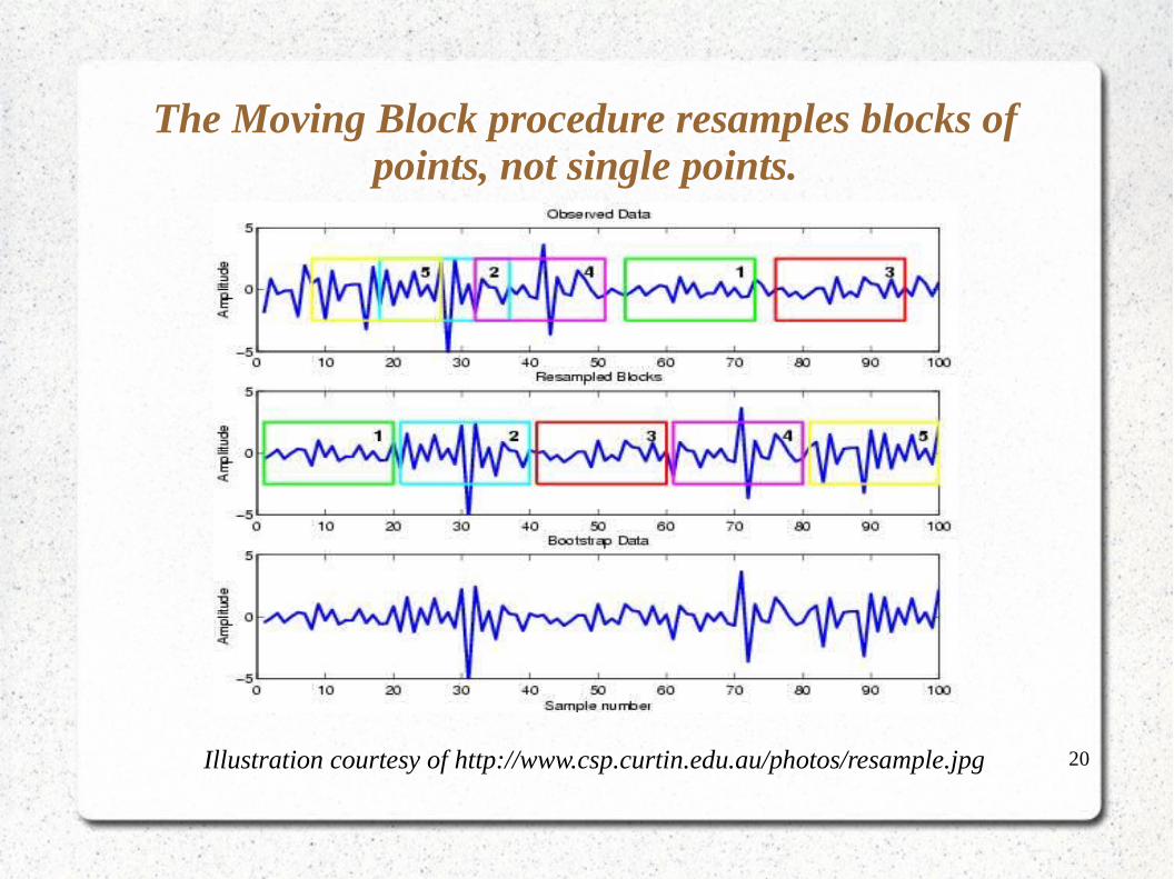
The Moving Block procedure resamples blocks of points, not single points.
Illustration courtesy of http://www.csp.curtin.edu.au/photos/resample.jpg
21
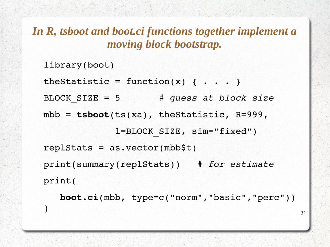
In R, tsboot and boot.ci functions together implement a moving block bootstrap.
library(boot)
theStatistic = function(x) { . . . }
BLOCK_SIZE = 5 # guess at block size
mbb = tsboot(ts(xa), theStatistic, R=999,
l=BLOCK_SIZE, sim="fixed")
replStats = as.vector(mbb$t)
print(summary(replStats)) # for estimate
print(
boot.ci(mbb, type=c("norm","basic","perc")) )
22
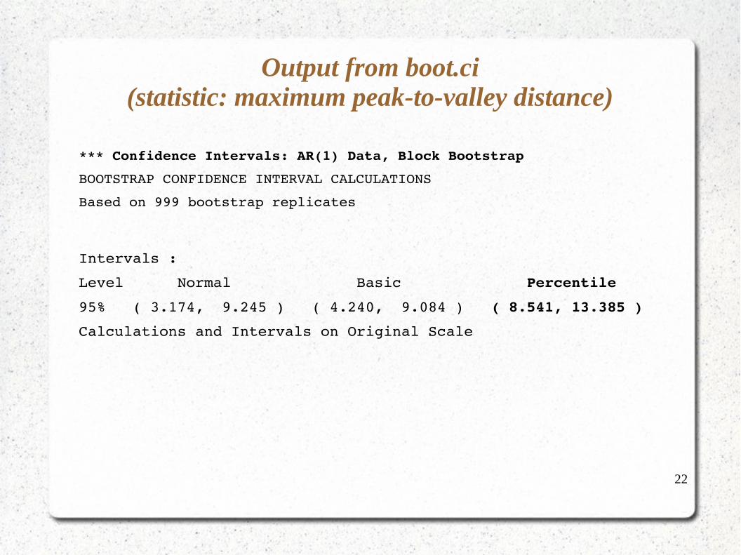
Output from boot.ci(statistic: maximum peak-to-valley distance)
*** Confidence Intervals: AR(1) Data, Block Bootstrap
BOOTSTRAP CONFIDENCE INTERVAL CALCULATIONS
Based on 999 bootstrap replicates
Intervals :
Level Normal Basic Percentile
95% ( 3.174, 9.245 ) ( 4.240, 9.084 ) ( 8.541, 13.385 )
Calculations and Intervals on Original Scale
23
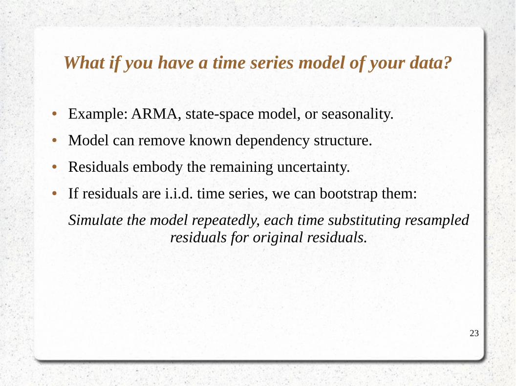
What if you have a time series model of your data?
● Example: ARMA, state-space model, or seasonality.
● Model can remove known dependency structure.
● Residuals embody the remaining uncertainty.
● If residuals are i.i.d. time series, we can bootstrap them:
Simulate the model repeatedly, each time substituting resampled residuals for original residuals.
24
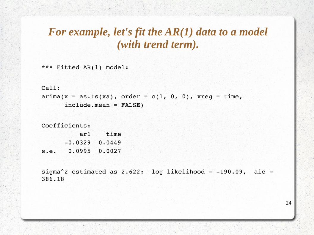
For example, let's fit the AR(1) data to a model (with trend term).
*** Fitted AR(1) model:
Call:arima(x = as.ts(xa), order = c(1, 0, 0), xreg = time, include.mean = FALSE)
Coefficients: ar1 time 0.0329 0.0449s.e. 0.0995 0.0027
sigma^2 estimated as 2.622: log likelihood = 190.09, aic = 386.18
25
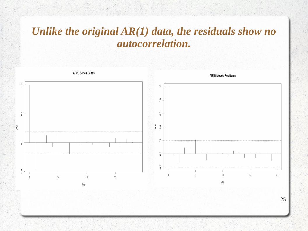
Unlike the original AR(1) data, the residuals show no autocorrelation.
26
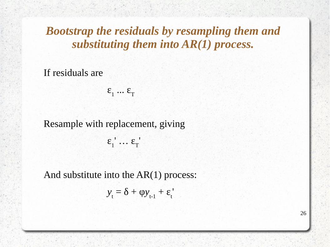
Bootstrap the residuals by resampling them and substituting them into AR(1) process.
If residuals are
ε1 ... ε
T
Resample with replacement, giving
ε1' … ε
T'
And substitute into the AR(1) process:
yt = δ + φy
t-1 + ε
t'
27
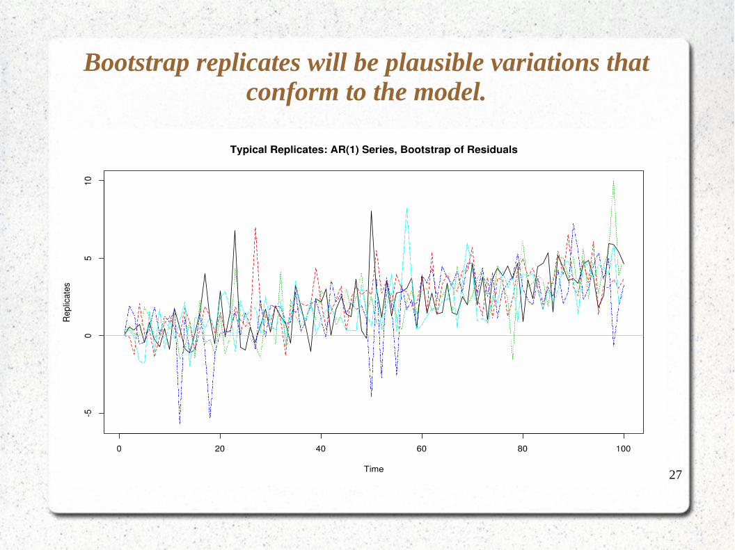
Bootstrap replicates will be plausible variations that conform to the model.
28
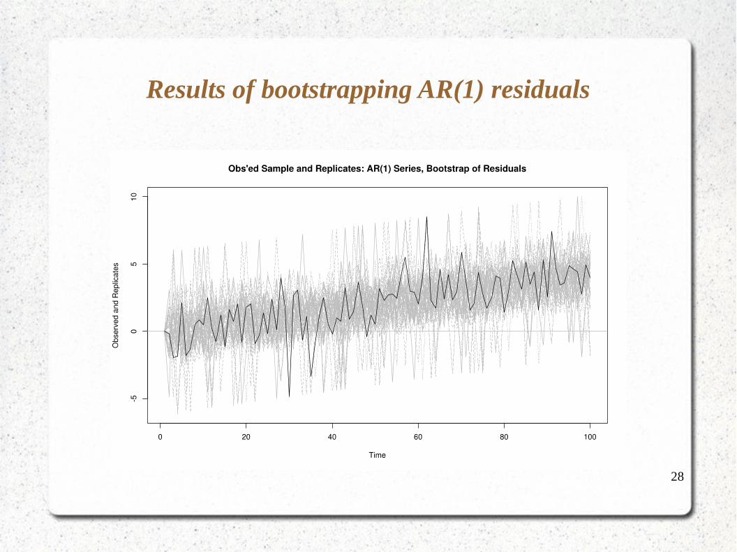
Results of bootstrapping AR(1) residuals
29
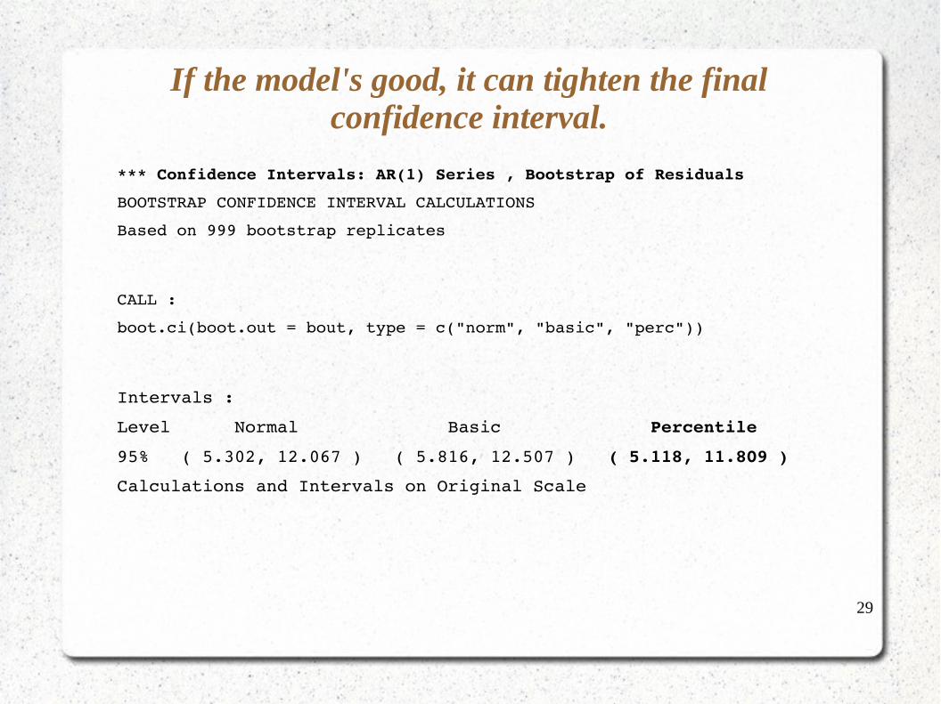
If the model's good, it can tighten the final confidence interval.
*** Confidence Intervals: AR(1) Series , Bootstrap of Residuals
BOOTSTRAP CONFIDENCE INTERVAL CALCULATIONS
Based on 999 bootstrap replicates
CALL :
boot.ci(boot.out = bout, type = c("norm", "basic", "perc"))
Intervals :
Level Normal Basic Percentile
95% ( 5.302, 12.067 ) ( 5.816, 12.507 ) ( 5.118, 11.809 )
Calculations and Intervals on Original Scale
30
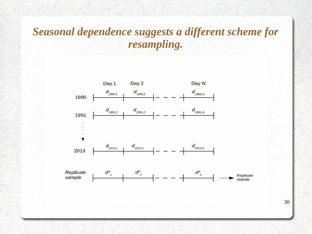
Seasonal dependence suggests a different scheme for resampling.
31
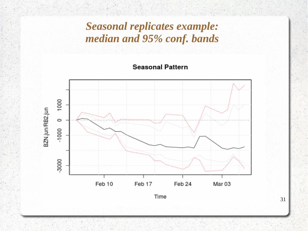
Seasonal replicates example:median and 95% conf. bands
32
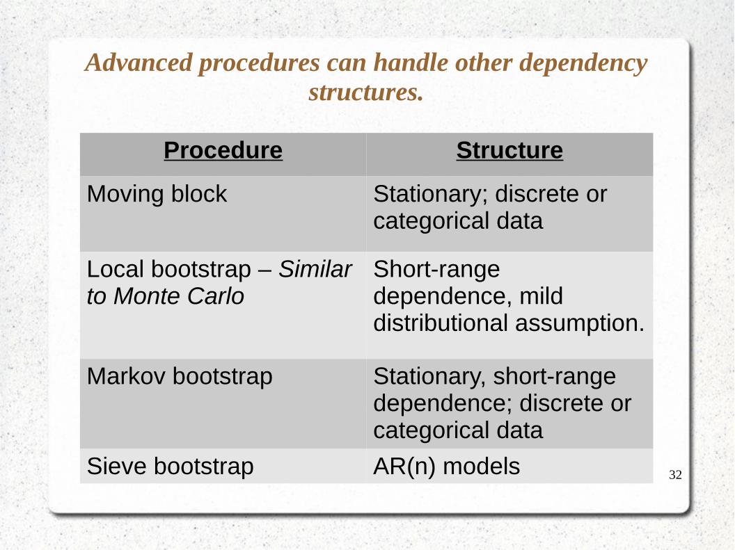
Advanced procedures can handle other dependency structures.
Procedure Structure
Moving block Stationary; discrete or categorical data
Local bootstrap – Similar to Monte Carlo
Short-range dependence, mild distributional assumption.
Markov bootstrap Stationary, short-range dependence; discrete or categorical data
Sieve bootstrap AR(n) models
33
Is there a middle-ground between naïve bootstrap and full model?
● Naïve can be too naïve.
● Model is often unknown.
● Maximum Entropy bootstrap is alternative.
● Parametric bootstrap of differences.
● Maximum entropy distribution of differences – very mild assumption
● Preserves many properties, including shape, seasonality, even some non-stationarity
34
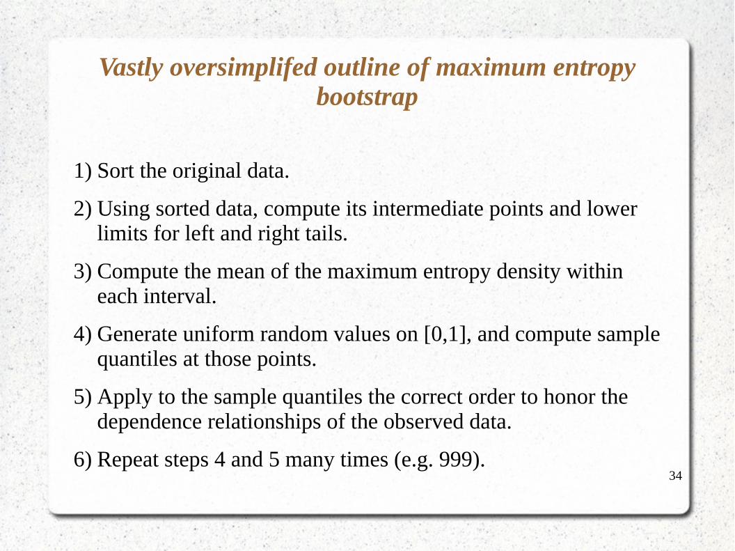
Vastly oversimplifed outline of maximum entropy bootstrap
1) Sort the original data.
2) Using sorted data, compute its intermediate points and lower limits for left and right tails.
3) Compute the mean of the maximum entropy density within each interval.
4) Generate uniform random values on [0,1], and compute sample quantiles at those points.
5) Apply to the sample quantiles the correct order to honor the dependence relationships of the observed data.
6) Repeat steps 4 and 5 many times (e.g. 999).
35
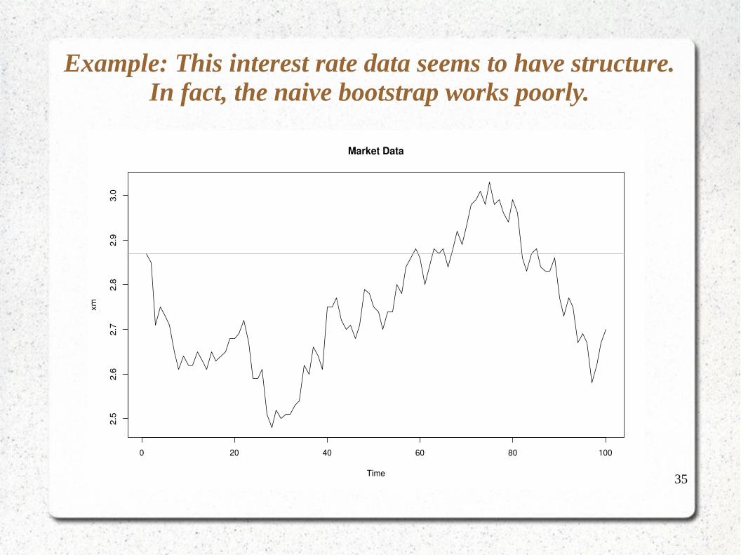
Example: This interest rate data seems to have structure. In fact, the naive bootstrap works poorly.
36
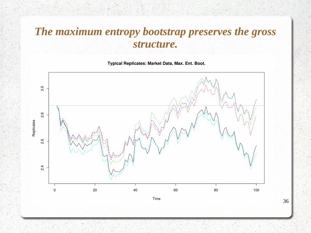
The maximum entropy bootstrap preserves the gross structure.
37
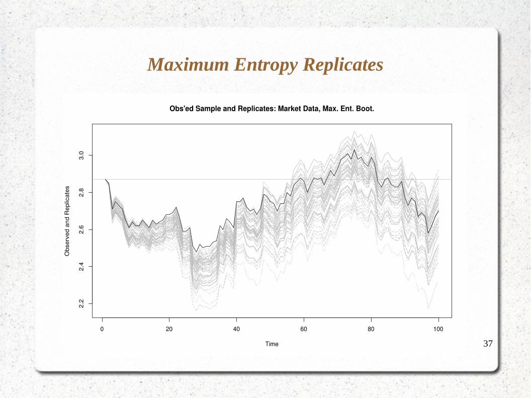
Maximum Entropy Replicates
38
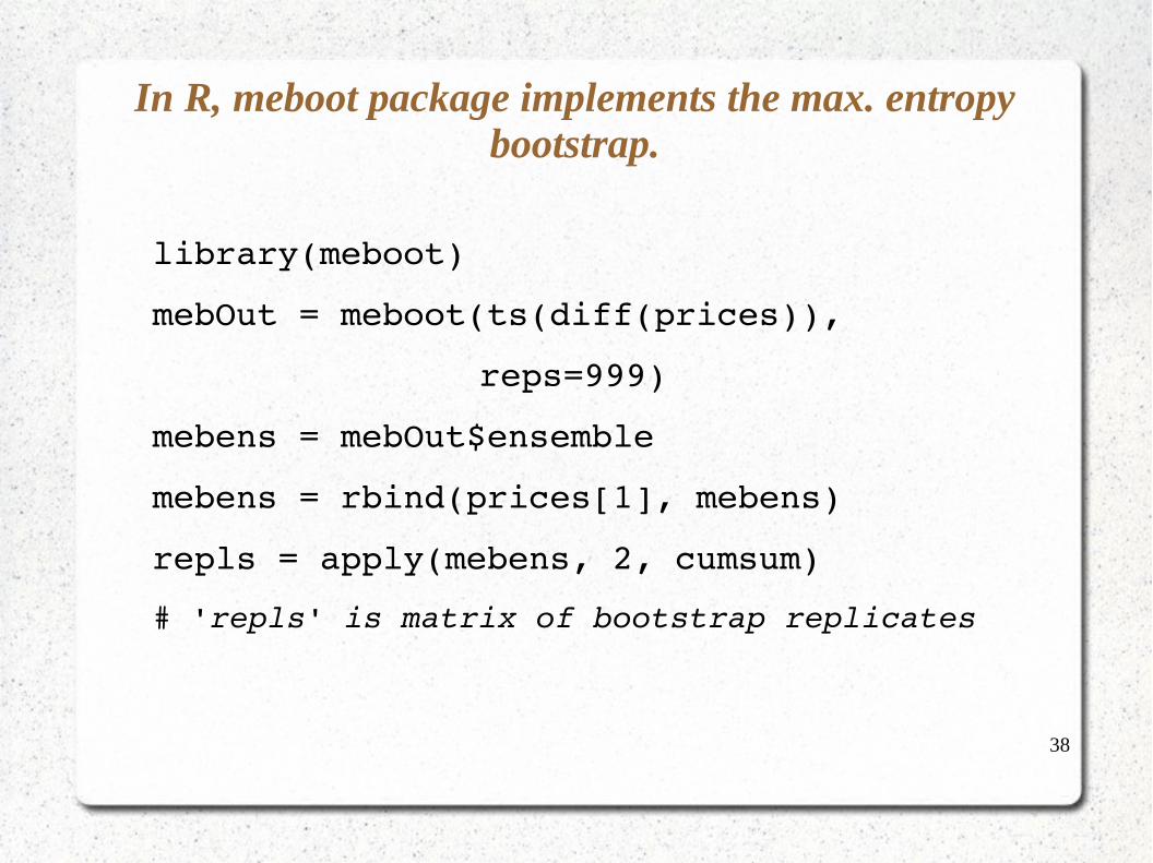
In R, meboot package implements the max. entropy bootstrap.
library(meboot)
mebOut = meboot(ts(diff(prices)),
reps=999)
mebens = mebOut$ensemble
mebens = rbind(prices[1], mebens)
repls = apply(mebens, 2, cumsum)
# 'repls' is matrix of bootstrap replicates
39
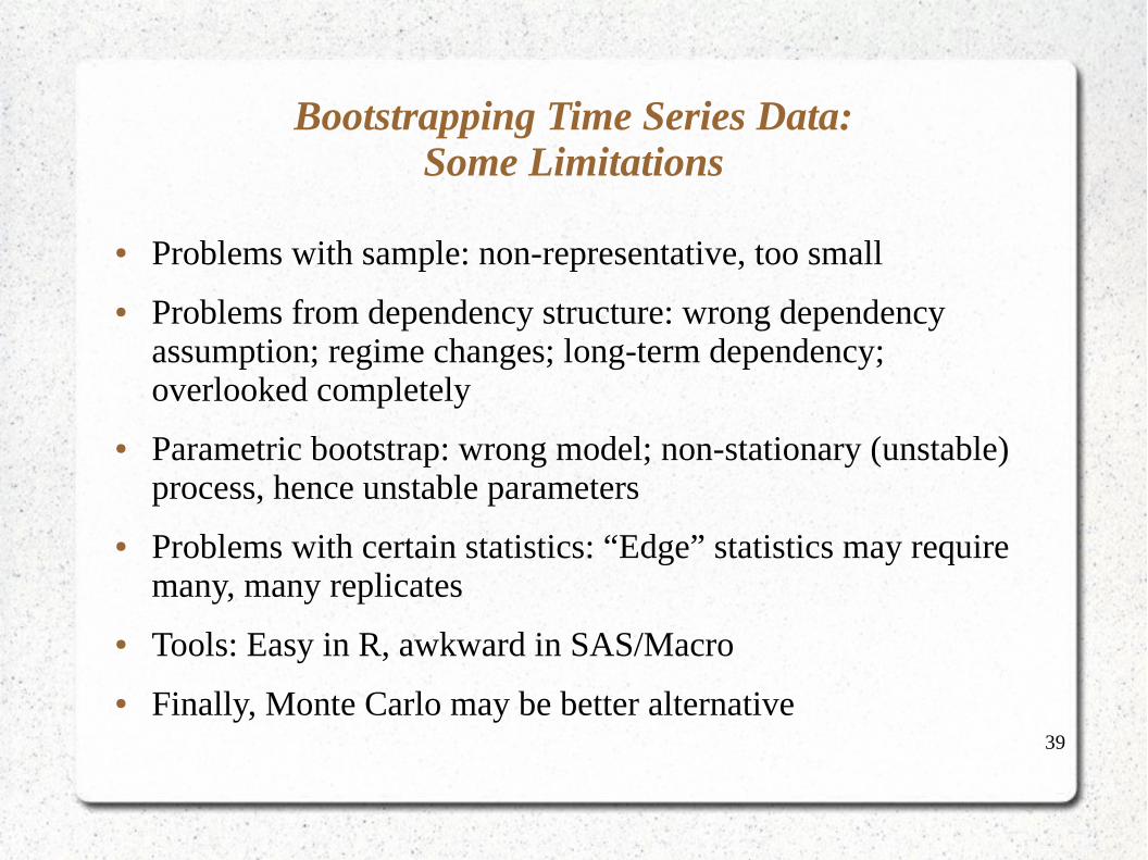
Bootstrapping Time Series Data:Some Limitations
● Problems with sample: non-representative, too small
● Problems from dependency structure: wrong dependency assumption; regime changes; long-term dependency; overlooked completely
● Parametric bootstrap: wrong model; non-stationary (unstable) process, hence unstable parameters
● Problems with certain statistics: “Edge” statistics may require many, many replicates
● Tools: Easy in R, awkward in SAS/Macro
● Finally, Monte Carlo may be better alternative
40
Some References
● An Introduction to the Bootstrap by Efron and Tibshirani
● Bootstrap Methods and Their Applications by Davison and Hinkley
● “The Moving Blocks Bootstrap Versus Parametric Time Series Models”, Vogel and Shallcross, Water Resources Research (June 1996)
● “Bootstraps for Time Series”, Bühlmann, Statistical Science (2002, No. 1)
● “Maximum Entropy Bootstrap for Time Series”, Vinod and López-de-Lacalle, J. of Stat. Soft. (Jan 2009)
41
Thank you!
Talk materials available at
http://bit.ly/csp2015teetor
Recommended