æORDINARY DIFFERENTIAL EQUATIONSAND LINEAR ALGEBRA
— THE LECTURE NOTES FOR MATH-263 (2009)

ORDINARY DIFFERENTIAL EQUATIONSAND LINEAR ALGEBRA
JIAN-JUN XU
Department of Mathematics and Statistics, McGill University
Kluwer Academic PublishersBoston/Dordrecht/London
Contents
1. INTRODUCTION 11 Definitions and Basic Concepts 1
1.1 Ordinary Differential Equation (ODE) 11.2 Solution 11.3 Order n of the DE 11.4 Initial Conditions 21.5 First Order Equation and Direction Field 21.6 Linear Equation: 21.7 Homogeneous Linear Equation: 31.8 Partial Differential Equation (PDE) 31.9 General Solution of a Linear Differential Equation 31.10 A System of ODE’s 4
2 The Approaches of Finding Solutions of ODE 52.1 Analytical Approaches 52.2 Numerical Approaches 5
2. FIRST ORDER DIFFERENTIAL EQUATIONS 71 Linear Equation 7
1.1 Linear homogeneous equation 81.2 Linear inhomogeneous equation 8
2 Nonlinear Equations (I) 102.1 Separable Equations. 102.2 Logistic Equation 122.3 Fundamental Existence and Uniqueness Theorem 142.4 Bernoulli Equation: 162.5 Homogeneous Equation: 16
v
vi ORDINARY DIFFERENTIAL EQUATIONS AND LINEAR ALGEBRA
3 Nonlinear Equations (II)— Exact Equation and IntegratingFactor 183.1 Exact Equations. 183.2 Theorem. 20
4 Integrating Factors. 205 Linear Equations 22
5.1 Basic Concepts and General Properties 225.1.1 Linearity 225.1.2 Superposition of Solutions 235.1.3 Kernel of Linear operator L(y) 245.2 New Notations 24
6 Basic Theory of Linear Differential Equations 246.1 Basics of Linear Vector Space 256.1.1 Dimension and Basis of Vector Space 256.1.2 Linear Independency 266.2 Wronskian of n-functions 276.2.1 Definition 276.2.2 Theorem 1 286.2.3 Theorem 2 286.2.4 The Solutions of L[y] = 0 as a Linear Vector Space 30
7 Linear Equations 317.1 Basic Concepts and General Properties 317.1.1 Linearity 317.1.2 Superposition of Solutions 327.1.3 Kernel of Linear operator L(y) 327.2 New Notations 32
8 Basic Theory of Linear Differential Equations 338.1 Basics of Linear Vector Space 348.1.1 Dimension and Basis of Vector Space 348.1.2 Linear Independency 348.2 Wronskian of n-functions 358.2.1 Definition 358.2.2 Theorem 1 368.2.3 Theorem 2 378.2.4 The Solutions of L[y] = 0 as a Linear Vector Space 39
9 Solutions for Equations with Constants Coefficients —The Method with Undetermined Parameters 399.1 The Method with Undetermined Parameters 39
Contents vii
9.2 Basic Equalities (I) 399.3 Cases (I) ( r1 > r2) 409.4 Cases (II) ( r1 = r2 ) 419.5 Cases (III) ( r1,2 = λ± iµ) 43
10 Finding a Particular Solution for Inhomogeneous Equation44
10.1 The Method of Variation of Parameters 4410.2 Reduction of Order 48
11 Solutions for Equations with Variable Coefficients 5111.1 Euler Equations 5111.2 Cases (I) ( r1 6= r2) 5211.3 Cases (II) ( r1 = r2 ) 5211.4 Cases (III) ( r1,2 = λ± iµ) 5311.5 (*)Exact Equations 54
3. LAPLACE TRANSFORMS 551 Introduction 552 Laplace Transform 57
2.1 Definition 572.1.1 Piecewise Continuous Function 572.1.2 Laplace Transform 572.2 Existence of Laplace Transform 57
3 Basic Properties and Formulas ofLaplace Transform 583.1 Linearity of Laplace Transform 583.2 Laplace Transforms for f(t) = eat 583.3 Laplace Transforms for f(t) = {sin(bt) and cos(bt)}
583.4 Laplace Transforms for {eatf(t); f(bt)} 593.5 Laplace Transforms for {tnf(t)} 593.6 Laplace Transforms for {f ′(t)} 60
4 Inverse Laplace Transform 604.1 Theorem: 604.2 Definition 61
5 Solve IVP of DE’s with Laplace Transform Method 615.1 Example 1 615.2 Example 2 635.3 Example 3 64
6 Further Studies of Laplace Transform 65
viii ORDINARY DIFFERENTIAL EQUATIONS AND LINEAR ALGEBRA
6.1 Step Function 656.1.1 Definition 656.1.2 Some basic operations with the step function 656.1.3 Laplace Transform of Unit Step Function 666.2 Impulse Function 726.2.1 Definition 726.2.2 Laplace Transform of Impulse Function 736.3 Convolution Integral 746.3.1 Theorem 746.3.2 The properties of convolution integral 74
4. SOLUTIONS OF SYSTEMS OF LINEARALGEBRAIC EQUATIONS 771 Introduction 772 Introduction 773 Solutions for general (m× n) System of Linear Equations 77
3.1 (*)Elementary Row Operations 793.2 Gaussian Elimination 813.3 Gauss-Jordan Elimination 823.4 (*)General Algorithm for Gaussian Elimination with
Pivoting 833.5 Existence and Uniqueness of Solution 84
5. MATRICES AND DETERMINANTS 851 Matrix Algebra 85
1.1 Matrix Addition 851.2 Scalar Multiplication of Matrix 851.3 Matrix Multiplication 851.4 Some Properties of Matrix Multiplication 86
2 Some Important (n× n) Matrices 863 Partitioning of Matrices 874 Transpose Matrix 885 The Inverse of a Square Matrix 896 Basic Theorems on the Inverse of Matrix 907 Determinant 91
7.1 Basic concepts and Definition of Determinant 927.2 Theorems of Determinant 947.3 Properties of Determinant 957.4 Minor, Co-factors, Adjoint 97
Contents ix
8 Cramer’s Rule 1009 L-U Factorization 101
6. VECTOR SPACE—DEFINITIONS AND BASIC CONCEPTS 1031 Introduction and Motivation 103
1.1 A brief Review of Geometric Vectors in 3D space 1032 Definition of a Vector Space 1053 Examples of Vector Spaces 1064 Subspaces 1075 Linear Combinations and Spanning Sets 1076 Linear Dependence and Independence 1087 Bases and Dimensions 108
7. INNER PRODUCT SPACES 1131 Introduction 113
1.1 Definition of Inner Product in Rn 1141.1.1 Schwarz Inequality 1141.1.2 Triangle Inequality 1151.2 Basic Properties of the Inner Product in Rn 115
2 Definition of a Real Inner Product Space 1153 Definition of a Complex Inner Product Space 1164 (*)The Gram-Schmidt Orthogonalization Procedure 118
8. LINEAR TRANSFORMATIONS 1231 Introduction 1232 Definitions 123
2.1 Matrix Representation of Linear Transformation 1252.2 The Kernel and Range of a Linear Transformation 126
3 (*)Inverse Transformation 129
9. EIGENVALUES AND EIGENVECTORS 1331 Introduction 1332 Definitions 1333 General Results for Eigenvalues and Eigenvectors 1394 Symmetric Matrices 1425 Diagonalization 144
10. EIGENVECTOR METHOD 1471 Introduction 147
x ORDINARY DIFFERENTIAL EQUATIONS AND LINEAR ALGEBRA
2 (n×n) System of Linear Equations and Eigenvector Method1492.1 (2× 2) System of Linear Equations 1502.2 Case 1: ∆ > 0 1502.3 Case 2: ∆ < 0 1522.4 Case 3: ∆ = 0 153
3 Stability of Solutions 1563.1 Definition of Stability 1563.2 Case 1: ∆ > 0 1573.3 Case 2: ∆ < 0 1583.4 Case 3: ∆ = 0 160
4 Solutions for (n× n) Homogeneous Linear System 1614.1 Case (I): (A) is non-defective matrix 1624.2 Case (II): (A) has a pair of complex conjugate
eigen-values 1644.3 Case (III): (A) is a defective matrix 164
5 Solutions for Non-homogeneous Linear System 1665.1 Variation of Parameters Method 167
Appendices 169ASSIGNMENTS AND SOLUTIONS 169


Chapter 1
INTRODUCTION
1. Definitions and Basic Concepts1.1 Ordinary Differential Equation (ODE)
An equation involving the derivatives of an unknown function y of asingle variable x over an interval x ∈ (I).
1.2 SolutionAny function y = f(x) which satisfies this equation over the interval
(I) is called a solution of the ODE.For example, y = e2x is a solution of the ODE
y′ = 2y
and y = sin(x2) is a solution of the ODE
xy′′ − y′ + 4x3y = 0.
In general, ODE has infinitely many solutions, depending on a numberof constants.
1.3 Order n of the DEAn ODE is said to be order n, if y(n) is the highest order derivative
occurring in the equation. The simplest first order ODE is y′ = g(x).The most general form of an n-th order ODE is
F (x, y, y′, . . . , y(n)) = 0
with F a function of n + 2 variables x, u0, u1, . . . , un. The equations
xy′′ + y = x3, y′ + y2 = 0, y′′′ + 2y′ + y = 0
1
2 ORDINARY DIFFERENTIAL EQUATIONS AND LINEAR ALGEBRA
are examples of ODE’s of second order, first order and third order re-spectively with respectively
F (x, u0, u1, u2) = xu2 + u0 − x3,
F (x, u0, u1) = u1 + u20,
F (x, u0, u1, u2, u3) = u3 + 2u1 + u0.
In general, the solutions of n-th order equation may depend on con-stants.
1.4 Initial ConditionsTo determine a specific solution, one may impose some initial condi-
tions (IC’s):
y(x0) = y0, y′(x0) = y′0, · · · , y(n−1)(x0) = y(n−1)0 .
1.5 First Order Equation and Direction FieldGiven
y′(x) = F (x, y), (x, y) ∈ R.
Let R : a ≤ x ≤ b, c ≤ y ≤ d be a rectangular domain, and set
a = x0 < x1 < · · · < xm = b
be equally spaced poind in [a, b] and
c = y0 < y1 < · · · < yn = d
be equally spaced poind in [c, d]. Then (xi, yj), 0 ≤ i ≤ m, 0 ≤ j ≤n form a rectangular grid. Through each point Pi,j in the grid, wedraw a short line segment with the slope F (xi, yj). The result is anapproximation of direction field of the ODE in R.
If the grid points are sufficiently close together, we can draw approxi-mate integral curve of the equation by drawing curves through points inthe grid tangent to the line segments associated with the points in thegrid.
1.6 Linear Equation:If the function F is linear in the variables u0, u1, . . . , un the ODE is
said to be linear. If, in addition, F is homogeneous then the ODE is saidto be homogeneous. The first of the above examples above is linear arelinear, the second is non-linear and the third is linear and homogeneous.
INTRODUCTION 3
The general n-th order linear ODE can be written
an(x) dnydxn + an−1(x) dn−1y
dxn−1 + · · ·+ a1(x) dydx
+a0(x)y = b(x).
1.7 Homogeneous Linear Equation:The linear DE is homogeneous, if and only if b(x) ≡ 0. Linear homo-
geneous equations have the important property that linear combinationsof solutions are also solutions. In other words, if y1, y2, . . . , ym are solu-tions and c1, c2, . . . , cm are constants then
c1y1 + c2y2 + · · ·+ cmym
is also a solution.
1.8 Partial Differential Equation (PDE)An equation involving the partial derivatives of a function of more
than one variable is called PED. The concepts of linearity and homo-geneity can be extended to PDE’s. The general second order linear PDEin two variables x, y is
a(x, y)∂2u∂x2 + b(x, y) ∂2u
∂x∂y + c(x, y)∂2u∂y2 + d(x, y)∂u
∂x
+e(x, y)∂u∂y + f(x, y)u = g(x, y).
Laplace’s equation∂2u
∂x2 +∂2u
∂y2 = 0
is a linear, homogeneous PDE of order 2. The functions u = log(x2+y2),u = xy, u = x2−y2 are examples of solutions of Laplace’s equation. Wewill not study PDE’s systematically in this course.
1.9 General Solution of a Linear DifferentialEquation
It represents the set of all solutions, i.e., the set of all functions whichsatisfy the equation in the interval (I).
For example, the general solution of the differential equation
y′ = 3x2
isy = x3 + C,
4 ORDINARY DIFFERENTIAL EQUATIONS AND LINEAR ALGEBRA
where C is an arbitrary constant. The constant C is the value of yat x = 0. This initial condition completely determines the solution.More generally, one easily shows that given a, b there is a unique solutiony of the differential equation with y(a) = b. Geometrically, this meansthat the one-parameter family of curves y = x2 +C do not intersect oneanother and they fill up the plane R2.
1.10 A System of ODE’s
y′1 = G1(x, y1, y2, . . . , yn)y′2 = G2(x, y1, y2, . . . , yn)...y′n = Gn(x, y1, y2, . . . , yn)
An n-th order ODE of the form y(n) = G(x, y, y′, . . . , yn−1) can be trans-formed in the form of the system of first order DE’s. If we introducedependant variables y1 = y, y2 = y′, . . . , yn = yn−1 we obtain the equiv-alent system of first order equations
y′1 = y2,y′2 = y3,...y′n = G(x, y1, y2, . . . , yn).
For example, the ODE y′′ = y is equivalent to the system
y′1 = y2,y′2 = y1.
In this way the study of n-th order equations can be reduced to thestudy of systems of first order equations. Some times, one called thelatter as the normal form of the n-th order ODE. Systems of equationsarise in the study of the motion of particles. For example, if P (x, y) isthe position of a particle of mass m at time t, moving in a plane underthe action of the force field (f(x, y), g(x, y), we have
md2xdt2
= f(x, y),md2y
dt2= g(x, y).
This is a second order system.The general first order ODE in normal form is
y′ = F (x, y).
INTRODUCTION 5
If F and ∂F∂y are continuous one can show that, given a, b, there is a
unique solution with y(a) = b. Describing this solution is not an easytask and there are a variety of ways to do this. The dependence of thesolution on initial conditions is also an important question as the initialvalues may be only known approximately.
The non-linear ODE yy′ = 4x is not in normal form but can bebrought to normal form
y′ =4x
y.
by dividing both sides by y.
2. The Approaches of Finding Solutions of ODE2.1 Analytical Approaches
Analytical solution methods: finding the exact form of solutions;
Geometrical methods: finding the qualitative behavior of solutions;
Asymptotic methods: finding the asymptotic form of the solution,which gives good approximation of the exact solution.
2.2 Numerical ApproachesNumerical algorithms — numerical methods;
Symbolic manipulators — Maple, MATHEMATICA, MacSyma.
This course mainly discuss the analytical approaches and mainly onanalytical solution methods.

Chapter 2
FIRST ORDER DIFFERENTIAL EQUATIONS
In this lecture we will treat linear and separable first order ODE’s.
1. Linear EquationThe general first order ODE has the form F (x, y, y′) = 0 where y =
y(x). If it is linear it can be written in the form
a0(x)y′ + a1(x)y = b(x)
where a0(x), a(x), b(x) are continuous functions of x on some interval(I).
To bring it to normal form y′ = f(x, y) we have to divide both sides ofthe equation by a0(x). This is possible only for those x where a0(x) 6= 0.After possibly shrinking I we assume that a0(x) 6= 0 on (I). So ourequation has the form (standard form)
y′ + p(x)y = q(x)
withp(x) = a1(x)/a0(x), q(x) = b(x)/a0(x),
both continuous on (I). Solving for y′ we get the normal form for alinear first order ODE, namely
y′ = q(x)− p(x)y.
7
8 ORDINARY DIFFERENTIAL EQUATIONS AND LINEAR ALGEBRA
1.1 Linear homogeneous equationLet us first consider the simple case: q(x) = 0, namely,
dy
dx+ p(x)y = 0.
With the chain law of derivative, one may write
y′(x)y
=ddx
ln [y(x)] = −p(x),
integrating both sides, we derive
ln y(x) = −∫
p(x)dx + C,
ory = C1e−
∫p(x)dx,
where C, as well as C1 = eC , is arbitrary constant.
1.2 Linear inhomogeneous equationWe now consider the general case:
dy
dx+ p(x)y = q(x).
We multiply the both sides of our differential equation with a factorµ(x) 6= 0. Then our equation is equivalent (has the same solutions) tothe equation
µ(x)y′(x) + µ(x)p(x)y(x) = µ(x)q(x).
We wish that with a properly chosen function µ(x),
µ(x)y′(x) + µ(x)p(x)y(x) =ddx
[µ(x)y(x)].
For this purpose, the function µ(x) must has the property
µ′(x) = p(x)µ(x), (2.1)
and µ(x) 6= 0 for all x. By solving the linear homogeneous equation(2.1), one obtain
µ(x) = e∫
p(x)dx. (2.2)
FIRST ORDER DIFFERENTIAL EQUATIONS 9
With this function, which is called an integrating factor, our equationis reduced to
ddx
[µ(x)y(x)] = µ(x)q(x), (2.3)
Integrating both sides, we get
µ(x)y =∫
µ(x)q(x)dx + C
with C an arbitrary constant. Solving for y, we get
y =1
µ(x)
∫µ(x)q(x)dx +
C
µ(x)= yP (x) + yH(x) (2.4)
as the general solution for the general linear first order ODE
y′ + p(x)y = q(x).
In solution (2.4):
the first part, yP (x): a particular solution of the inhomogeneousequation,
the second part, yH(x): the general solution of the associatedhomogeneous equation.
Note that for any pair of scalars a, b with a in (I), there is a uniquescalar C such that y(a) = b. Geometrically, this means that the solutioncurves y = φ(x) are a family of non-intersecting curves which fill theregion I ×R.
Example 1: Given
y′ + xy = x, (I) = R.
This is a linear first order ODE in standard form with p(x) = q(x) = x.The integrating factor is
µ(x) = e∫
xdx = ex2/2.
Hence, after multiplying both sides of our differential equation, we get
ddx
(ex2/2y) = xex2/2
which, after integrating both sides, yields
ex2/2y =∫
xex2/2dx + C = ex2/2 + C.
10 ORDINARY DIFFERENTIAL EQUATIONS AND LINEAR ALGEBRA
Hence the general solution is y = 1 + Ce−x2/2.
The solution satisfying the initial condition: y(0) = 1:
y = 1, (C = 0);
and
the solution satisfying I.C., y(0) = a:
y = 1 + (a− 1)e−x2/2, (C = a− 1).
Example 2: Given
xy′ − 2y = x3 sinx, (I) = (x > 0).
We bring this linear first order equation to standard form by dividingby x. We get
y′ − 2x
y = x2 sinx.
The integrating factor is
µ(x) = e∫−2dx/x = e−2 ln x = 1/x2.
After multiplying our DE in standard form by 1/x2 and simplifying, weget
ddx
(y/x2) = sinx
from which y/x2 = − cosx + C, and
y = −x2 cosx + Cx2. (2.5)
Note that (2.5) are a family of solutions to the DE
xy′ − 2y = x3 sinx
and that they all satisfy the initial condition y(0) = 0. This non-uniqueness is due to the fact that x = 0 is a singular point of theDE.
2. Nonlinear Equations (I)2.1 Separable Equations.
The first order ODE y′ = f(x, y) is said to be separable if f(x, y) canbe expressed as a product of a function of x times a function of y. TheDE then has the form:
y′ = g(x)h(y)
FIRST ORDER DIFFERENTIAL EQUATIONS 11
and, dividing both sides by h(y), it becomes
y′
h(y)= g(x).
Of course this is not valid for those solutions y = y(x) at the pointswhere h[y(x)] = 0. Assuming the continuity of g and h, we can integrateboth sides of the equation to get
∫y′(x)
h[y(x)]dx =
∫g(x)dx + C.
Assume that
H(y) =∫ dy
h(y),
By chain rule, we have
ddx
H[y(x)] = H ′(y)y′(x) =1
h[y(x)]y′(x),
hence
H[y(x)] =∫
y′(x)h[y(x)]
dx =∫
g(x)dx + C.
Therefore, ∫ dy
h(y)= H(y) =
∫g(x)dx + C,
gives the implicit form of the solution. It determines the value of yimplicitly in terms of x.
Example 1: y′ = x−5y2 .
To solve it using the above method we multiply both sides of theequation by y2 to get
y2y′ = (x− 5).
Integrating both sides we get y3/3 = x2/2− 5x + C. Hence,
y =[3x2/2− 15x + C1
]1/3.
Example 2: y′ = y−1x+3 (x > −3). By inspection, y = 1 is a solution.
Dividing both sides of the given DE by y − 1 we get
y′
y − 1=
1x + 3
.
12 ORDINARY DIFFERENTIAL EQUATIONS AND LINEAR ALGEBRA
This will be possible for those x where y(x) 6= 1. Integrating both sideswe get ∫
y′
y − 1dx =
∫ dx
x + 3+ C1,
from which we get ln |y− 1| = ln(x + 3) + C1. Thus |y− 1| = eC1(x + 3)from which y − 1 = ±eC1(x + 3). If we let C = ±eC1 , we get
y = 1 + C(x + 3).
Since y = 1 was found to be a solution by inspection the general solutionis
y = 1 + C(x + 3),
where C can be any scalar. For any (a, b) with a 6= −3, there is only onemember of this family which passes through (a, b).
However, it is seen that there is a family of lines passing through(−3, 1), while no solution line passing through (−3, b) with b 6= 1). Here,x = −3 is a singular point.
Example 3: y′ = y cos x1+2y2 . Transforming in the standard form then
integrating both sides we get∫ (1 + 2y2)
ydy =
∫cosxdx + C,
from which we get a family of the solutions:
ln |y|+ y2 = sinx + C,
where C is an arbitrary constant. However, this is not the general solu-tion of the equation, as it does not contains, for instance, the solution:y = 0. With I.C.: y(0)=1, we get C = 1, hence, the solution:
ln |y|+ y2 = sin x + 1.
2.2 Logistic Equation
y′ = ay(b− y),
where a, b > 0 are fixed constants. This equation arises in the studyof the growth of certain populations. Since the right-hand side of theequation is zero for y = 0 and y = b, the given DE has y = 0 and y = bas solutions. More generally, if y′ = f(t, y) and f(t, c) = 0 for all t insome interval (I), the constant function y = c on (I) is a solution ofy′ = f(t, y) since y′ = 0 for a constant function y.
FIRST ORDER DIFFERENTIAL EQUATIONS 13
To solve the logistic equation, we write it in the form
y′
y(b− y)= a.
Integrating both sides with respect to t we get∫
y′dt
y(b− y)= at + C
which can, since y′dt = dy, be written as∫ dy
y(b− y)= at + C.
Since, by partial fractions,
1y(b− y)
=1b(1y
+1
b− y)
we obtain1b(ln |y| − ln |b− y|) = at + C.
Multiplying both sides by b and exponentiating both sides to the basee, we get
|y||b− y| = ebCeabt = C1eabt,
where the arbitrary constant C1 = ±ebC can be determined by the initialcondition (IC): y(0) = y0 as
C1 =|y0|
|b− y0| .
Two cases need to be discussed separately.
Case (I), y0 < b: one has C1 = | y0
b−y0| = y0
b−y0> 0. So that,
|y||b− y| =
(y0
b− y0
)eabt > 0, (t ∈ (I)).
From the above we derive
y/(b− y) = C1eabt,
y = (b− y)C1eabt.
14 ORDINARY DIFFERENTIAL EQUATIONS AND LINEAR ALGEBRA
This gives
y =bC1eabt
1 + C1eabt=
b(
y0
b−y0
)eabt
1 +(
y0
b−y0
)eabt
.
It shows that if y0 = 0, one has the solution y(t) = 0. However, if0 < y0 < b, one has the solution 0 < y(t) < b, and as t →∞, y(t) → b.
Case (II), y0 > b: one has C1 = | y0
b−y0| = − y0
b−y0> 0. So that,
∣∣∣∣y
b− y
∣∣∣∣ =(
y0
y0 − b
)eabt > 0, (t ∈ (I)).
From the above we derive
y/(y − b) =(
y0
y0 − b
)eabt,
y = (y − b)(
y0
y0 − b
)eabt.
This gives
y =b(
y0
y0−b
)eabt
(y0
y0−b
)eabt − 1
.
It shows that if y0 > b, one has the solution y(t) > b, and as t →∞,y(t) → b.
It is derived that
y(t) = 0 is an unstable equilibrium state of the system;
y(t) = b is a stable equilibrium state of the system.
2.3 Fundamental Existence and UniquenessTheorem
If the function f(x, y) together with its partial derivative with respectto y are continuous on the rectangle
(R) : |x− x0| ≤ a, |y − y0| ≤ b
there is a unique solution to the initial value problem
y′ = f(x, y), y(x0) = y0
defined on the interval |x− x0| < h where
h = min(a, b/M), M = max |f(x, y)|, (x, y) ∈ (R).
FIRST ORDER DIFFERENTIAL EQUATIONS 15
Note that this theorem indicates that a solution may not be definedfor all x in the interval |x− x0| ≤ a. For example, the function
y =bCeabx
1 + Ceabx
is solution to y′ = ay(b − y) but not defined when 1 + Ceabx = 0 eventhough f(x, y) = ay(b− y) satisfies the conditions of the theorem for allx, y.
The next example show why the condition on the partial derivativein the above theorem is important sufficient condition.
Consider the differential equation y′ = y1/3. Again y = 0 is a solution.Separating variables and integrating, we get
∫dy
y1/3= x + C1
which yieldsy2/3 = 2x/3 + C
and hencey = ±(2x/3 + C)3/2.
Taking C = 0, we get the solution
y = ±(2x/3)3/2, (x ≥ 0)
which along with the solution y = 0 satisfies y(0) = 0. Even more,Taking C = −(2x0/3)3/2, we get the solution:
y =
{0 (0 ≤ x ≤ x0)±[2(x− x0)/3]3/2, (x ≥ x0)
which also satisfies y(0) = 0. So the initial value problem
y′ = y1/3, y(0) = 0
does not have a unique solution. The reason this is so is due to the factthat
∂f
∂y(x, y) =
13y2/3
is not continuous when y = 0.
Many differential equations become linear or separable after a changeof variable. We now give two examples of this.
16 ORDINARY DIFFERENTIAL EQUATIONS AND LINEAR ALGEBRA
2.4 Bernoulli Equation:
y′ = p(x)y + q(x)yn (n 6= 1).
Note that y = 0 is a solution. To solve this equation, we set
u = yα,
where α is to be determined. Then, we have
u′ = αyα−1y′,
hence, our differential equation becomes
u′/α = p(x)u + q(x)yα+n−1. (2.6)
Now setα = 1− n,
Thus, (2.6) is reduced to
u′/α = p(x)u + q(x), (2.7)
which is linear. We know how to solve this for u from which we get solve
u = y1−n
to get
y = u1/(1−n). (2.8)
2.5 Homogeneous Equation:
y′ = F (y/x).
To solve this we letu = y/x,
so thaty = xu, and y′ = u + xu′.
Substituting for y, y′ in our DE gives
u + xu′ = F (u)
which is a separable equation. Solving this for u gives y via y = xu.
Note thatu ≡ a
FIRST ORDER DIFFERENTIAL EQUATIONS 17
is a solution ofxu′ = F (u)− u
whenever F (a) = a and that this gives
y = ax
as a solution ofy′ = f(y/x).
Example. y′ = (x− y)/x + y. This is a homogeneous equation since
x− y
x + y=
1− y/x
1 + y/x.
Setting u = y/x, our DE becomes
xu′ + u =1− u
1 + u
so that
xu′ =1− u
1 + u− u =
1− 2u− u2
1 + u.
Note that the right-hand side is zero if u = −1±√2. Separating variablesand integrating with respect to x, we get
∫ (1 + u)du
1− 2u− u2= ln |x|+ C1
which in turn gives
(−1/2) ln |1− 2u− u2| = ln |x|+ C1.
Exponentiating, we get
1√|1− 2u− u2| = eC1 |x|.
Squaring both sides and taking reciprocals, we get
u2 + 2u− 1 = C/x2
with C = ±1/e2C1 . This equation can be solved for u using the quadraticformula. If x0, y0 are given with
x0 6= 0, and u0 = y0/x0 6= −1
18 ORDINARY DIFFERENTIAL EQUATIONS AND LINEAR ALGEBRA
there is, by the fundamental, existence and uniqueness theorem, a uniquesolution with I.C.
y(x0) = y0.
For example, if x0 = 1, y0 = 2, we have, u(x0) = 2, so, C = 7 andhence
u2 + 2u− 1 = 7/x2
Solving for u, we get
u = −1 +√
2 + 7/x2
where the positive sign in the quadratic formula was chosen to makeu = 2, x = 1 a solution. Hence
y = −x + x√
2 + 7/x2 = −x +√
2x2 + 7
is the solution to the initial value problem
y′ =x− y
x + y, y(1) = 2
for x > 0 and one can easily check that it is a solution for all x. Moreover,using the fundamental uniqueness theorem, it can be shown thatit is the only solution defined for all x.
3. Nonlinear Equations (II)— Exact Equationand Integrating Factor
3.1 Exact Equations.By a region of the (x, y)-plane we mean a connected open subset of
the plane. The differential equation
M(x, y) + N(x, y)dy
dx= 0
is said to be exact on a region (R) if there is a function F (x, y) definedon (R) such that
∂F
∂x= M(x, y);
∂F
∂y= N(x, y)
In this case, if M,N are continuously differentiable on (R) we have
∂M
∂y=
∂N
∂x. (2.9)
FIRST ORDER DIFFERENTIAL EQUATIONS 19
Conversely, it can be shown that condition (2.9) is also sufficient for theexactness of the given DE on (R) providing that (R) is simply connected,.i.e., has no “holes”.
The exact equations are solvable. In fact, suppose y(x) is its solution.Then one can write:
M [x, y(x)] + N [x, y(x)]dy
dx=
∂F
∂x+
∂F
∂y
dy
dx
=ddx
F [x, y(x)] = 0.
It follows thatF [x, y(x)] = C,
where C is an arbitrary constant. This is an implicit form of the solutiony(x). Hence, the function F (x, y), if it is found, will give a family of thesolutions of the given DE.
The curves F (x, y) = C are called integral curves of the given DE.
Example 1. 2x2y dydx + 2xy2 + 1 = 0. Here
M = 2xy2 + 1, N = 2x2y
and R = R2, the whole (x, y)-plane. The equation is exact on R2 sinceR2 is simply connected and
∂M
∂y= 4xy =
∂N
∂x.
To find F we have to solve the partial differential equations
∂F
∂x= 2xy2 + 1,
∂F
∂y= 2x2y.
If we integrate the first equation with respect to x holding y fixed, weget
F (x, y) = x2y2 + x + φ(y).
Differentiating this equation with respect to y gives
∂F
∂y= 2x2y + φ′(y) = 2x2y
using the second equation. Hence φ′(y) = 0 and φ(y) is a constantfunction. The solutions of our DE in implicit form is
x2y2 + x = C.
20 ORDINARY DIFFERENTIAL EQUATIONS AND LINEAR ALGEBRA
Example 2. We have already solved the homogeneous DE
dy
dx=
x− y
x + y.
This equation can be written in the form
y − x + (x + y)dy
dx= 0
which is an exact equation. In this case, the solution in implicit form is
x(y − x) + y(x + y) = C,
i.e.,y2 + 2xy − x2 = C.
3.2 Theorem.If F (x, y) is homogeneous of degree n then
x∂F
∂x+ y
∂F
∂y= nF (x, y).
Proof. The function F is homogeneous of degree n, if
F (tx, ty) = tnF (x, y).
Differentiating this with respect to t and setting t = 1 yields the result.QED
4. Integrating Factors.If the differential equation M +Ny′ = 0 is not exact it can sometimes
be made exact by multiplying it by a continuously differentiable functionµ(x, y). Such a function is called an integrating factor. An integratingfactor µ satisfies the PDE:
∂µM
∂y=
∂µN
∂x,
which can be written in the form(
∂M
∂y− ∂N
∂x
)µ = N
∂µ
∂x−M
∂µ
∂y.
This equation can be simplified in special cases, two of which we treatnext.
FIRST ORDER DIFFERENTIAL EQUATIONS 21
µ is a function of x only. This happens if and only if
∂M∂y − ∂N
∂x
N= p(x)
is a function of x only in which case µ′ = p(x)µ.
µ is a function of y only. This happens if and only if
∂M∂y − ∂N
∂x
M= q(y)
is a function of y only in which case µ′ = −q(y)µ.
µ = P (x)Q(y) . This happens if and only if
∂M
∂y− ∂N
∂x= p(x)N − q(y)M, (2.10)
where
p(x) =P ′(x)P (x)
, q(y) =Q′(y)Q(y)
.
If the system really permits the functions p(x), q(y), such that (2.10)hold, then we can derive
P (x) = ±e∫
p(x)dx; Q(y) = ±e∫
q(y)dy.
Example 1. 2x2 + y + (x2y − x)y′ = 0. Here
∂M∂y − ∂N
∂x
N=
2− 2xy
x2y − x=−2x
so that there is an integrating factor µ(x) which is a function of x only,and satisfies
µ′ = −2µ/x.
Hence µ = 1/x2 is an integrating factor and
2 + y/x2 + (y − 1/x)y′ = 0
is an exact equation whose general solution is
2x− y/x + y2/2 = C
22 ORDINARY DIFFERENTIAL EQUATIONS AND LINEAR ALGEBRA
or2x2 − y + xy2/2 = Cx.
Example 2. y + (2x− yey)y′ = 0. Here
∂M∂y − ∂N
∂x
M=−1y
,
so that there is an integrating factor which is a function of y only whichsatisfies
µ′ = µ/y.
Hence y is an integrating factor and
y2 + (2xy − y2ey)y′ = 0
is an exact equation with general solution:
xy2 + (−y2 + 2y − 2)ey = C.
A word of caution is in order here. The solutions of the exact DEobtained by multiplying by the integrating factor may havesolutions which are not solutions of the original DE. This is dueto the fact that µ may be zero and one will have to possibly excludethose solutions where µ vanishes. However, this is not the case for theabove Example 2.
5. Linear EquationsIn this chapter, we are only concerned with linear equations.
5.1 Basic Concepts and General PropertiesLet us now go to linear equations. The general form is
L(y) =
a0(x)y(n) + a1(x)y(n−1) + · · ·+ an(x)y = b(x). (2.11)
The function L is called a differential operator.
5.1.1 LinearityThe characteristic features of linear operator L is that
With any constants (C1, C2),
L(C1y1 + C2y2) = C1L(y1) + C2L(y2).
FIRST ORDER DIFFERENTIAL EQUATIONS 23
With any given functions of x, p1(x), p2(x), and the Linear operators,
L1(y) = a0(x)y(n) + a1(x)y(n−1) + · · ·+ an(x)y
L2(y) = b0(x)y(n) + b1(x)y(n−1) + · · ·+ bn(x)y,
the functionp1L1 + p2L2
defined by
(p1L1 + p2L2)(y) = p1(x)L1(y) + p2(x)L2(y)
=[p(x)a0(x) + p2(x)b0(x)
]y(n) + · · ·
+ [p1(x)an(x) + p2(x)bn(x)] y
is again a linear differential operator.
Linear operators in general are subject to the distributive law:
L(L1 + L2) = LL1 + LL2,
(L1 + L2)L = L1L + L2L.
5.1.2 Superposition of SolutionsThe solutions the linear of equation (10.3) have the following proper-
ties:
For any two solutions y1, y2 of (10.3), namely,
L(y1) = b(x), L(y2) = b(x),
the difference (y1 − y2) is a solution of the associated homogeneousequation
L(y) = 0.
For any pair of of solutions y1, y2 of the associated homogenous equa-tion:
L(y1) = 0, L(y2) = 0,
the linear combination(a1y1 + a2y2)
of solutions y1, y2 is again a solution of the homogenous equation:
L(y) = 0.
24 ORDINARY DIFFERENTIAL EQUATIONS AND LINEAR ALGEBRA
5.1.3 Kernel of Linear operator L(y)The solution space of L(y) = 0 is also called the kernel of L and is
denoted by ker(L). It is a subspace of the vector space of real valuedfunctions on some interval I. If yp is a particular solution of
L(y) = b(x),
the general solution ofL(y) = b(x)
isker(L) + yp = {y + yp | L(y) = 0}.
5.2 New NotationsThe differential operator
{L(y) = y′} =⇒ Dy.
The operatorL(y) = y′′ = D2y = D ◦Dy,
where ◦ denotes composition of functions. More generally, the operator
L(y) = y(n) = Dny.
The identity operator I is defined by
I(y) = y = D0y.
By definition D0 = I. The general linear n-th order ODE can thereforebe written
[a0(x)Dn + a1(x)Dn−1 + · · ·+ an(x)I
](y) = b(x).
6. Basic Theory of Linear DifferentialEquations
In this section we will develop the theory of linear differential equa-tions. The starting point is the fundamental existence theorem for thegeneral n-th order ODE L(y) = b(x), where
L(y) = Dn + a1(x)Dn−1 + · · ·+ an(x).
We will also assume that a0(x) 6= 0, a1(x), . . . , an(x), b(x) are continuousfunctions on the interval I.
FIRST ORDER DIFFERENTIAL EQUATIONS 25
The fundamental theory says that for any x0 ∈ I, the initial valueproblem
L(y) = b(x)
with the initial conditions:
y(x0) = d1, y′(x0) = d2, . . . , y
(n−1)(x0) = dn
has a unique solution for any (d1, d2, . . . , dn) ∈ Rn.From the above, one may deduce that the general solution of n-th
order linear equation contains n arbitrary constants. So that, we mayintroduce the concept of fundamental solutions for n-th order lin-ear equation. Given a set of n solutions: {y1(x), · · · yn(x)} of theequation, if any solution y(x) of the equation can be expressed in theform:
y(x) = c1y1(x) + · · ·+ cnyn(x),
with a proper set of constants {c1, · · · , cn}, then the solutions {yi(x), i =1, 2, · · · , n} is called a set of fundamental solutions.
6.1 Basics of Linear Vector Space6.1.1 Dimension and Basis of Vector Space
We call the vector space being n-dimensional with the notation bydim(V ) = n. This means that there exists a sequence of elements:y1, y2, . . . , yn ∈ V such that every y ∈ V can be uniquely written in theform
y = c1y1 + c2y2 + . . . cnyn
with c1, c2, . . . , cn ∈ R. Such a sequence of elements of a vector spaceV is called a basis for V . In the context of DE’s it is also known as afundamental set. The number of elements in a basis for V is calledthe dimension of V and is denoted by dim(V ). For instance,
e1 = (1, 0, . . . , 0), e2 = (0, 1, . . . , 0), . . . ,en = (0, 0, . . . , 1)
is the standard basis of geometric vector space Rn.A set of vectors v1, v2, · · · , vn in a vector space V is said to span or
generate V if every v ∈ V can be written in the form
v = c1v1 + c2v2 + · · ·+ cnvn
with c1, c2, . . . , cn ∈ R. Obviously, not any set of n vectors can spanthe vector space V . It will be seen that {v1, v2, · · · , vn} span the vectorspace V , if and only if they are linear independent.
26 ORDINARY DIFFERENTIAL EQUATIONS AND LINEAR ALGEBRA
6.1.2 Linear IndependencyThe vectors v1, v2, . . . , vn are said to be linearly independent if
c1v1 + c2v2 + . . . cnvn = 0
implies that the scalars c1, c2, . . . , cn are all zero. A basis can also becharacterized as a linearly independent generating set since the unique-ness of representation is equivalent to linear independence. More pre-cisely,
c1v1 + c2v2 + · · ·+ cnvn = c′1v1 + c′2v2 + · · ·+ c′nvn
impliesci = c′i for all i,
if and only if v1, v2, . . . , vn are linearly independent.To justify the linear independency of {v1(x), v2(x), v3(x)}, one may
pick any three point (x1, x2, x3) ∈ (I), we may derive a system linearequations:
c1v1(xi) + c2v2(xi) + c3v3(xi) = 0, (i = 1, 2, 3).
If the determinant of the coefficients of above equations is
∆ =
∣∣∣∣∣∣
v1(x1) v2(x1) v3(x1)v1(x2) v2(x2) v3(x2)v1(x3) v2(x3) v3(x3)
∣∣∣∣∣∣6= 0,
we derive c1 = c2 = c3 = 0. The set of function is linear independent.As an example of a linearly independent set of functions, consider
cos(x), cos(2x), sin(3x).
To prove their linear independence, suppose that c1, c2, c3 are scalarssuch that
c1 cos(x) + c2 cos(2x) + c3 sin(3x) = 0for all x. Then setting x = 0, π/2, π, we get
c1 + c2 = 0,−c2 = 0,−c1 + c2 − c3 = 0,
from which ∆ 6= 0, hence c1 = c2 = c3 = 0. The set of function is (L.I.)An example of a linearly dependent set is
sin2(x), cos2(x), cos(2x)
sincecos(2x) = cos2(x)− sin2(x)
implies thatcos(2x) + sin2(x) + (−1) cos2(x) = 0.
FIRST ORDER DIFFERENTIAL EQUATIONS 27
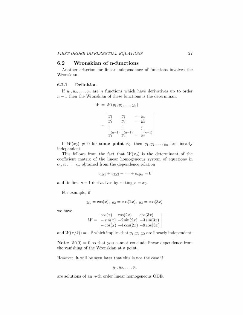
6.2 Wronskian of n-functionsAnother criterion for linear independence of functions involves the
Wronskian.
6.2.1 DefinitionIf y1, y2, . . . , yn are n functions which have derivatives up to order
n− 1 then the Wronskian of these functions is the determinant
W = W (y1, y2, . . . , yn)
=
∣∣∣∣∣∣∣∣∣∣
y1 y2 . . . yn
y′1 y′2 . . . y′n...
......
y(n−1)1 y
(n−1)2 . . . y
(n−1)n
∣∣∣∣∣∣∣∣∣∣
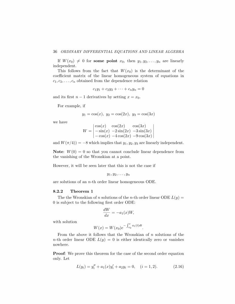
If W (x0) 6= 0 for some point x0, then y1, y2, . . . , yn are linearlyindependent.
This follows from the fact that W (x0) is the determinant of thecoefficient matrix of the linear homogeneous system of equations inc1, c2, . . . , cn obtained from the dependence relation
c1y1 + c2y2 + · · ·+ cnyn = 0
and its first n− 1 derivatives by setting x = x0.
For example, if
y1 = cos(x), y2 = cos(2x), y3 = cos(3x)
we have
W =
∣∣∣∣∣∣
cos(x) cos(2x) cos(3x)− sin(x) −2 sin(2x) −3 sin(3x)− cos(x) −4 cos(2x) −9 cos(3x)
∣∣∣∣∣∣
and W (π/4)) = −8 which implies that y1, y2, y3 are linearly independent.
Note: W (0) = 0 so that you cannot conclude linear dependence fromthe vanishing of the Wronskian at a point.
However, it will be seen later that this is not the case if
y1, y2, . . . , yn
are solutions of an n-th order linear homogeneous ODE.
28 ORDINARY DIFFERENTIAL EQUATIONS AND LINEAR ALGEBRA
6.2.2 Theorem 1The the Wronskian of n solutions of the n-th order linear ODE L(y) =
0 is subject to the following first order ODE:
dW
dx= −a1(x)W,
with solutionW (x) = W (x0)e
−∫ x
x0a1(t)dt
.
From the above it follows that the Wronskian of n solutions of then-th order linear ODE L(y) = 0 is either identically zero or vanishesnowhere.
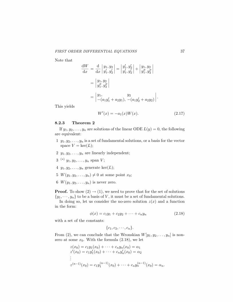
Proof: We prove this theorem for the case of the second order equationonly. Let
L(yi) = y′′i + a1(x)y′i + a2yi = 0, (i = 1, 2). (2.12)
Note that
dW
dx=
ddx
∣∣∣∣y1, y2
y′1, y′2
∣∣∣∣ =∣∣∣∣y′1, y′2y′1, y′2
∣∣∣∣ +∣∣∣∣y1, y2
y′′1 , y′′2
∣∣∣∣
=∣∣∣∣y1, y2
y′′1 , y′′2
∣∣∣∣
=∣∣∣∣y1, y2
−(a1y′1 + a2y1), −(a1y
′2 + a2y2)
∣∣∣∣ .
This yields
W ′(x) = −a1(x)W (x). (2.13)
6.2.3 Theorem 2If y1, y2, . . . , yn are solutions of the linear ODE L(y) = 0, the following
are equivalent:
1 y1, y2, . . . , yn is a set of fundamental solutions, or a basis for the vectorspace V = ker(L);
2 y1, y2, . . . , yn are linearly independent;
3 (∗) y1, y2, . . . , yn span V ;
4 y1, y2, . . . , yn generate ker(L);
FIRST ORDER DIFFERENTIAL EQUATIONS 29
5 W (y1, y2, . . . , yn) 6= 0 at some point x0;
6 W (y1, y2, . . . , yn) is never zero.
Proof. To show (2) → (1), we need to prove that for the set of solutions{y1, · · · , yn} to be a basis of V , it must be a set of fundamental solutions.
In doing so, let us consider the no-zero solution z(x) and a functionin the form:
φ(x) = c1y1 + c2y2 + · · ·+ cnyn (2.14)
with a set of the constants:
{c1, c2, · · · , cn}.
From (2), we can conclude that the Wronskian W [y1, y2, . . . , yn] is non-zero at some x0. With the formula (2.18), we let
z(x0) = c1y1(x0) + · · ·+ cnyn(x0) = α1
z′(x0) = c1y′1(x0) + · · ·+ cny′n(x0) = α2
...z(n−1)(x0) = c1y
(n−1)1 (x0) + · · ·+ cny
(n−1)n (x0) = αn.
The above linear system we may determine a set of the constants:
{c1, c2, · · · , cn},
since its determinantW (x0) 6= 0.
The above results yield that the two solutions z(x) and φ(x) satisfythe same initial conditions at x = x0. From the theorem of uniquenessof solution, it follows that
z(x) ≡ φ(x), for all x ∈ (I).
The proof of (2) → (5) follows from the fact that if the Wronskian werezero at some point x0, the set of solutions {y1, · · · , yn} must be lineardependent.
In fact, with arbitrary {c1, c2, · · · , cn} let us consider the solution
φ(x) = c1y1 + c2y2 + · · ·+ cnyn,
30 ORDINARY DIFFERENTIAL EQUATIONS AND LINEAR ALGEBRA
and set up the following homogeneous system of equations
φ(x0) = c1y1(x0) + · · ·+ cnyn(x0) = 0φ′(x0) = c1y
′1(x0) + · · ·+ cny′n(x0) = 0
...φ(n−1)(x0) = c1y
(n−1)1 (x0) + · · ·+ cny
(n−1)n (x0) = 0.
Since the Wronskian W (x0) = 0, the above system must have a set ofnon-zero solution, would have a non-zero solution for {c1, c2, · · · , cn}.However, on the other hand, the function φ(x) is the solution of L(x) =0 with the zero initial conditions. From the fundamental theorem ofexistence and uniqueness, we deduce that
φ(x) = c1y1 + c2y2 + · · ·+ cnyn ≡ 0.
This implied y1, y2, . . . , yn are linearly dependent.QED
From the above, we see that to solve the n-th order linear DE L(y) =b(x) we first find linear n independent solutions y1, y2, . . . , yn of L(y) = 0.Then, if yP is a particular solution of L(y) = b(x), the general solutionof L(y) = b(x) is
y = c1y1 + c2y2 + · · ·+ cnyn + yP .
The initial conditions:
y(x0) = d1, y′(x0) = d2, . . . , y
(n−1)n (x0) = dn
then determine the constants c1, c2, . . . , cn uniquely.
6.2.4 The Solutions of L[y] = 0 as a Linear Vector SpaceSuppose that v1(x), v2(x), · · · , vn(x) are the linear independent solu-
tions of linear equation L[y] = 0. Then any solution of this equation canbe written in the form
v(x) = c1v1 + c2v2 + · · ·+ cnvn
with c1, c2, . . . , cn ∈ R. Especially The zero function v(x) = 0 is alsosolution. The all solutions of linear homogeneous equation form a vectorspace V with the basis
v1(x), v2(x), · · · , vn(x).
The vector space V consists of all possible linear combinations of thevectors:
{v1, v2, . . . , vn}.
FIRST ORDER DIFFERENTIAL EQUATIONS 31
7. Linear EquationsIn this chapter, we are only concerned with linear equations.
7.1 Basic Concepts and General PropertiesLet us now go to linear equations. The general form is
L(y) =
a0(x)y(n) + a1(x)y(n−1) + · · ·+ an(x)y = b(x). (2.15)
The function L is called a differential operator.
7.1.1 LinearityThe characteristic features of linear operator L is that
With any constants (C1, C2),
L(C1y1 + C2y2) = C1L(y1) + C2L(y2).
With any given functions of x, p1(x), p2(x), and the Linear operators,
L1(y) = a0(x)y(n) + a1(x)y(n−1) + · · ·+ an(x)y
L2(y) = b0(x)y(n) + b1(x)y(n−1) + · · ·+ bn(x)y,
the function
p1L1 + p2L2
defined by
(p1L1 + p2L2)(y) = p1(x)L1(y) + p2(x)L2(y)
=[p(x)a0(x) + p2(x)b0(x)
]y(n) + · · ·
+ [p1(x)an(x) + p2(x)bn(x)] y
is again a linear differential operator.
Linear operators in general are subject to the distributive law:
L(L1 + L2) = LL1 + LL2,
(L1 + L2)L = L1L + L2L.
32 ORDINARY DIFFERENTIAL EQUATIONS AND LINEAR ALGEBRA
7.1.2 Superposition of SolutionsThe solutions the linear of equation (10.3) have the following proper-
ties:
For any two solutions y1, y2 of (10.3), namely,
L(y1) = b(x), L(y2) = b(x),
the difference (y1 − y2) is a solution of the associated homogeneousequation
L(y) = 0.
For any pair of of solutions y1, y2 of the associated homogenous equa-tion:
L(y1) = 0, L(y2) = 0,
the linear combination(a1y1 + a2y2)
of solutions y1, y2 is again a solution of the homogenous equation:
L(y) = 0.
7.1.3 Kernel of Linear operator L(y)The solution space of L(y) = 0 is also called the kernel of L and is
denoted by ker(L). It is a subspace of the vector space of real valuedfunctions on some interval I. If yp is a particular solution of
L(y) = b(x),
the general solution ofL(y) = b(x)
isker(L) + yp = {y + yp | L(y) = 0}.
7.2 New NotationsThe differential operator
{L(y) = y′} =⇒ Dy.
The operatorL(y) = y′′ = D2y = D ◦Dy,
where ◦ denotes composition of functions. More generally, the operator
L(y) = y(n) = Dny.
FIRST ORDER DIFFERENTIAL EQUATIONS 33
The identity operator I is defined by
I(y) = y = D0y.
By definition D0 = I. The general linear n-th order ODE can thereforebe written
[a0(x)Dn + a1(x)Dn−1 + · · ·+ an(x)I
](y) = b(x).
8. Basic Theory of Linear DifferentialEquations
In this section we will develop the theory of linear differential equa-tions. The starting point is the fundamental existence theorem for thegeneral n-th order ODE L(y) = b(x), where
L(y) = Dn + a1(x)Dn−1 + · · ·+ an(x).
We will also assume that a0(x) 6= 0, a1(x), . . . , an(x), b(x) are continuousfunctions on the interval I.The fundamental theory says that for any x0 ∈ I, the initial valueproblem
L(y) = b(x)
with the initial conditions:
y(x0) = d1, y′(x0) = d2, . . . , y
(n−1)(x0) = dn
has a unique solution y = y(x) for any (d1, d2, . . . , dn) ∈ Rn.From the above, one may deduce that the general solution of n-th
order linear equation contains n arbitrary constants. It can be alsodeduced that the above solution can be expressed in the form:
y(x) = d1y1(x) + · · ·+ dnyn(x),
where the yi(x), (i = 1, 2, · · · , n) is the set of the solutions for the IVPwith IC’s: {
y(i−1)(x0) = 1, i = 1, 2, · · ·n)y(k−1)(x0) = 0, (k 6= i, 1 ≤ k ≤ n).
In general, if the equation L(y) = 0 has a set of n solutions: {y1(x), · · · yn(x)}of the equation, such that solution y(x) of the equation can be expressedin the form:
y(x) = c1y1(x) + · · ·+ cnyn(x),
with a proper set of constants {c1, · · · , cn}, then the solutions {yi(x), i =1, 2, · · · , n} is called a set of fundamental solutions of the equation.
34 ORDINARY DIFFERENTIAL EQUATIONS AND LINEAR ALGEBRA
8.1 Basics of Linear Vector Space8.1.1 Dimension and Basis of Vector Space
We call the vector space being n-dimensional with the notation bydim(V ) = n. This means that there exists a sequence of elements:y1, y2, . . . , yn ∈ V such that every y ∈ V can be uniquely written in theform
y = c1y1 + c2y2 + . . . cnyn
with c1, c2, . . . , cn ∈ R. Such a sequence of elements of a vector spaceV is called a basis for V . In the context of DE’s it is also known as afundamental set. The number of elements in a basis for V is calledthe dimension of V and is denoted by dim(V ). For instance,
e1 = (1, 0, . . . , 0), e2 = (0, 1, . . . , 0), . . . ,en = (0, 0, . . . , 1)
is the standard basis of geometric vector space Rn.A set of vectors v1, v2, · · · , vn in a vector space V is said to span or
generate V if every v ∈ V can be written in the form
v = c1v1 + c2v2 + · · ·+ cnvn
with c1, c2, . . . , cn ∈ R. Obviously, not any set of n vectors can spanthe vector space V . It will be seen that {v1, v2, · · · , vn} span the vectorspace V , if and only if they are linear independent.
8.1.2 Linear IndependencyThe vectors v1, v2, . . . , vn are said to be linearly independent if
c1v1 + c2v2 + . . . cnvn = 0
implies that the scalars c1, c2, . . . , cn are all zero. A basis can also becharacterized as a linearly independent generating set since the unique-ness of representation is equivalent to linear independence. More pre-cisely,
c1v1 + c2v2 + · · ·+ cnvn = c′1v1 + c′2v2 + · · ·+ c′nvn
impliesci = c′i for all i,
if and only if v1, v2, . . . , vn are linearly independent.To justify the linear independency of {v1(x), v2(x), v3(x)}, one may
pick any three point (x1, x2, x3) ∈ (I), we may derive a system linearequations:
c1v1(xi) + c2v2(xi) + c3v3(xi) = 0, (i = 1, 2, 3).
FIRST ORDER DIFFERENTIAL EQUATIONS 35
If the determinant of the coefficients of above equations is
∆ =
∣∣∣∣∣∣
v1(x1) v2(x1) v3(x1)v1(x2) v2(x2) v3(x2)v1(x3) v2(x3) v3(x3)
∣∣∣∣∣∣6= 0,
we derive c1 = c2 = c3 = 0. The set of function is linear independent.As an example of a linearly independent set of functions, consider
cos(x), cos(2x), sin(3x).
To prove their linear independence, suppose that c1, c2, c3 are scalarssuch that
c1 cos(x) + c2 cos(2x) + c3 sin(3x) = 0
for all x. Then setting x = 0, π/2, π, we get
c1 + c2 = 0,−c2 = 0,−c1 + c2 − c3 = 0,
from which ∆ 6= 0, hence c1 = c2 = c3 = 0. The set of function is (L.I.)An example of a linearly dependent set is
sin2(x), cos2(x), cos(2x)
sincecos(2x) = cos2(x)− sin2(x)
implies thatcos(2x) + sin2(x) + (−1) cos2(x) = 0.
8.2 Wronskian of n-functionsAnother criterion for linear independence of functions involves the
Wronskian.
8.2.1 DefinitionIf y1, y2, . . . , yn are n functions which have derivatives up to order
n− 1 then the Wronskian of these functions is the determinant
W = W (y1, y2, . . . , yn)
=
∣∣∣∣∣∣∣∣∣∣
y1 y2 . . . yn
y′1 y′2 . . . y′n...
......
y(n−1)1 y
(n−1)2 . . . y
(n−1)n
∣∣∣∣∣∣∣∣∣∣
36 ORDINARY DIFFERENTIAL EQUATIONS AND LINEAR ALGEBRA
If W (x0) 6= 0 for some point x0, then y1, y2, . . . , yn are linearlyindependent.
This follows from the fact that W (x0) is the determinant of thecoefficient matrix of the linear homogeneous system of equations inc1, c2, . . . , cn obtained from the dependence relation
c1y1 + c2y2 + · · ·+ cnyn = 0
and its first n− 1 derivatives by setting x = x0.
For example, if
y1 = cos(x), y2 = cos(2x), y3 = cos(3x)
we have
W =
∣∣∣∣∣∣
cos(x) cos(2x) cos(3x)− sin(x) −2 sin(2x) −3 sin(3x)− cos(x) −4 cos(2x) −9 cos(3x)
∣∣∣∣∣∣
and W (π/4)) = −8 which implies that y1, y2, y3 are linearly independent.
Note: W (0) = 0 so that you cannot conclude linear dependence fromthe vanishing of the Wronskian at a point.
However, it will be seen later that this is not the case if
y1, y2, . . . , yn
are solutions of an n-th order linear homogeneous ODE.
8.2.2 Theorem 1The the Wronskian of n solutions of the n-th order linear ODE L(y) =
0 is subject to the following first order ODE:
dW
dx= −a1(x)W,
with solutionW (x) = W (x0)e
−∫ x
x0a1(t)dt
.
From the above it follows that the Wronskian of n solutions of then-th order linear ODE L(y) = 0 is either identically zero or vanishesnowhere.
Proof: We prove this theorem for the case of the second order equationonly. Let
L(yi) = y′′i + a1(x)y′i + a2yi = 0, (i = 1, 2). (2.16)
FIRST ORDER DIFFERENTIAL EQUATIONS 37
Note thatdW
dx=
ddx
∣∣∣∣y1, y2
y′1, y′2
∣∣∣∣ =∣∣∣∣y′1, y′2y′1, y′2
∣∣∣∣ +∣∣∣∣y1, y2
y′′1 , y′′2
∣∣∣∣
=∣∣∣∣y1, y2
y′′1 , y′′2
∣∣∣∣
=∣∣∣∣y1, y2
−(a1y′1 + a2y1), −(a1y
′2 + a2y2)
∣∣∣∣ .
This yields
W ′(x) = −a1(x)W (x). (2.17)
8.2.3 Theorem 2If y1, y2, . . . , yn are solutions of the linear ODE L(y) = 0, the following
are equivalent:
1 y1, y2, . . . , yn is a set of fundamental solutions, or a basis for the vectorspace V = ker(L);
2 y1, y2, . . . , yn are linearly independent;
3 (∗) y1, y2, . . . , yn span V ;
4 y1, y2, . . . , yn generate ker(L);
5 W (y1, y2, . . . , yn) 6= 0 at some point x0;
6 W (y1, y2, . . . , yn) is never zero.
Proof. To show (2) → (1), we need to prove that for the set of solutions{y1, · · · , yn} to be a basis of V , it must be a set of fundamental solutions.
In doing so, let us consider the no-zero solution z(x) and a functionin the form:
φ(x) = c1y1 + c2y2 + · · ·+ cnyn (2.18)
with a set of the constants:
{c1, c2, · · · , cn}.From (2), we can conclude that the Wronskian W [y1, y2, . . . , yn] is non-zero at some x0. With the formula (2.18), we let
z(x0) = c1y1(x0) + · · ·+ cnyn(x0) = α1
z′(x0) = c1y′1(x0) + · · ·+ cny′n(x0) = α2
...z(n−1)(x0) = c1y
(n−1)1 (x0) + · · ·+ cny
(n−1)n (x0) = αn.
38 ORDINARY DIFFERENTIAL EQUATIONS AND LINEAR ALGEBRA
The above linear system we may determine a set of the constants:
{c1, c2, · · · , cn},since its determinant
W (x0) 6= 0.
The above results yield that the two solutions z(x) and φ(x) satisfythe same initial conditions at x = x0. From the theorem of uniquenessof solution, it follows that
z(x) ≡ φ(x), for all x ∈ (I).
The proof of (2) → (5) follows from the fact that if the Wronskian werezero at some point x0, the set of solutions {y1, · · · , yn} must be lineardependent.
In fact, with arbitrary {c1, c2, · · · , cn} let us consider the solution
φ(x) = c1y1 + c2y2 + · · ·+ cnyn,
and set up the following homogeneous system of equations
φ(x0) = c1y1(x0) + · · ·+ cnyn(x0) = 0φ′(x0) = c1y
′1(x0) + · · ·+ cny′n(x0) = 0
...φ(n−1)(x0) = c1y
(n−1)1 (x0) + · · ·+ cny
(n−1)n (x0) = 0.
Since the Wronskian W (x0) = 0, the above system must have a set ofnon-zero solution, would have a non-zero solution for {c1, c2, · · · , cn}.However, on the other hand, the function φ(x) is the solution of L(x) =0 with the zero initial conditions. From the fundamental theorem ofexistence and uniqueness, we deduce that
φ(x) = c1y1 + c2y2 + · · ·+ cnyn ≡ 0.
This implied y1, y2, . . . , yn are linearly dependent.QED
From the above, we see that to solve the n-th order linear DE L(y) =b(x) we first find linear n independent solutions y1, y2, . . . , yn of L(y) = 0.Then, if yP is a particular solution of L(y) = b(x), the general solutionof L(y) = b(x) is
y = c1y1 + c2y2 + · · ·+ cnyn + yP .
The initial conditions:
y(x0) = d1, y′(x0) = d2, . . . , y
(n−1)n (x0) = dn
then determine the constants c1, c2, . . . , cn uniquely.
FIRST ORDER DIFFERENTIAL EQUATIONS 39
8.2.4 The Solutions of L[y] = 0 as a Linear Vector SpaceSuppose that v1(x), v2(x), · · · , vn(x) are the linear independent solu-
tions of linear equation L[y] = 0. Then any solution of this equation canbe written in the form
v(x) = c1v1 + c2v2 + · · ·+ cnvn
with c1, c2, . . . , cn ∈ R. Especially The zero function v(x) = 0 is alsosolution. The all solutions of linear homogeneous equation form a vectorspace V with the basis
v1(x), v2(x), · · · , vn(x).
The vector space V consists of all possible linear combinations of thevectors:
{v1, v2, . . . , vn}.
9. Solutions for Equations with ConstantsCoefficients —The Method withUndetermined Parameters
In what follows, we shall first focus on the linear equations with con-stant coefficients:
L(y) = a0y(n) + a1y
(n−1) + · · ·+ any = b(x)
and present two different approaches to solve them.
9.1 The Method with Undetermined ParametersTo illustrate the idea, as a special case, let us first consider the 2-nd
order Linear equation with the constant coefficients:
L(y) = ay′′ + by′ + cy = f(x). (2.19)
The associate homogeneous equation is:
L(y) = ay′′ + by′ + cy = 0. (2.20)
9.2 Basic Equalities (I)We first give the following basic identities:
D(erx) = rerx; D2(erx) = r2erx;· · · Dn(erx) = rnerx. (2.21)
40 ORDINARY DIFFERENTIAL EQUATIONS AND LINEAR ALGEBRA
To solve this equation, we assume that the solution is in the formy(x) = erx, where r is a constant to be determined. Due to the propertiesof the exponential function erx:
y′(x) = ry(x); y′′(x) = r2y(x);
· · · y(n) = rny(x), (2.22)
we can write
L(erx) = φ(r)erx. (2.23)
for any given (r, x), where
φ(r) = ar2 + br + c.
is called the characteristic polynomial. From (2.23) it is seen that thefunction erx satisfies the equation (2.19), namely
L(erx) = 0,
as long as the constant r is the root of the characteristic polynomial, i.e.
φ(r) = 0.
In general, the polynomial φ(r) has two roots (r1, r2): One can write
φ(r) = ar2 + br + c = a(r − r1)(r − r2).
Accordingly, the equation (2.20) has two solutions:
{y1(x) = er1x; y2(x) = er2x}.Two cases should be discussed separately.
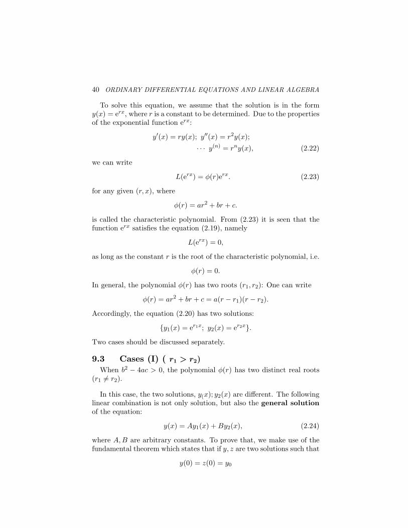
9.3 Cases (I) ( r1 > r2)
When b2 − 4ac > 0, the polynomial φ(r) has two distinct real roots(r1 6= r2).
In this case, the two solutions, y(x); y2(x) are different. The followinglinear combination is not only solution, but also the general solutionof the equation:
y(x) = Ay1(x) + By2(x), (2.24)
where A,B are arbitrary constants. To prove that, we make use of thefundamental theorem which states that if y, z are two solutions such that
y(0) = z(0) = y0
FIRST ORDER DIFFERENTIAL EQUATIONS 41
andy′(0) = z′(0) = y′0
then y = z. Let y be any solution and consider the linear equations inA,B
Ay1(0) + By2(0) = y(0),Ay′1(0) + By′2(0) = y′(0), (2.25)
or
A + B = y0,Ar1 + Br2 = y′0.
(2.26)
Due to r1 6= r2, these conditions leads to the unique solution A, B. Withthis choice of A, B the solution
z = Ay1 + By2
satisfiesz(0) = y(0), z′(0) = y′(0)
and hence y = z. Thus, (2.33) contains all possible solutions of theequation, so, it is indeed the general solution.
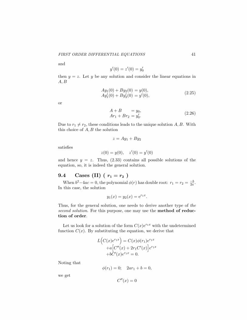
9.4 Cases (II) ( r1 = r2 )When b2−4ac = 0, the polynomial φ(r) has double root: r1 = r2 = −b
2a .In this case, the solution
y1(x) = y2(x) = er1x.
Thus, for the general solution, one needs to derive another type of thesecond solution. For this purpose, one may use the method of reduc-tion of order.
Let us look for a solution of the form C(x)er1x with the undeterminedfunction C(x). By substituting the equation, we derive that
L(C(x)er1x
)= C(x)φ(r1)er1x
+a[C ′′(x) + 2r1C
′(x)]er1x
+bC ′(x)er1x = 0.
Noting thatφ(r1) = 0; 2ar1 + b = 0,
we getC ′′(x) = 0
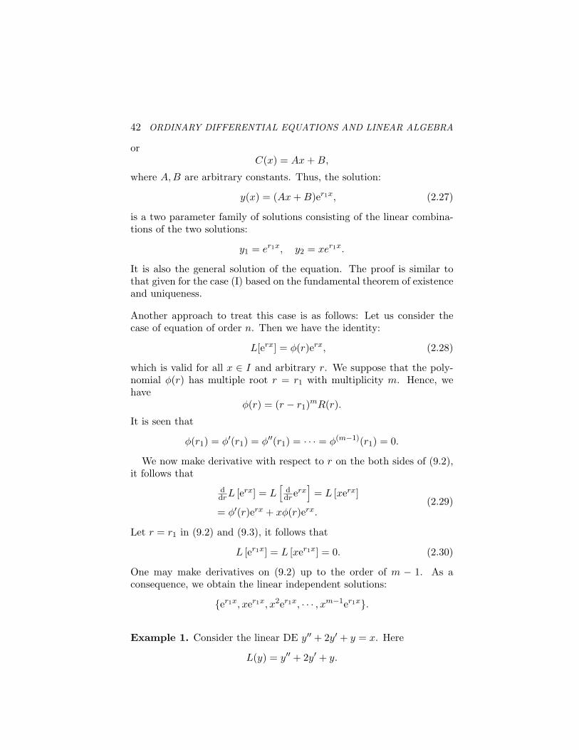
42 ORDINARY DIFFERENTIAL EQUATIONS AND LINEAR ALGEBRA
orC(x) = Ax + B,
where A,B are arbitrary constants. Thus, the solution:
y(x) = (Ax + B)er1x, (2.27)
is a two parameter family of solutions consisting of the linear combina-tions of the two solutions:
y1 = er1x, y2 = xer1x.
It is also the general solution of the equation. The proof is similar tothat given for the case (I) based on the fundamental theorem of existenceand uniqueness.
Another approach to treat this case is as follows: Let us consider thecase of equation of order n. Then we have the identity:
L[erx] = φ(r)erx, (2.28)
which is valid for all x ∈ I and arbitrary r. We suppose that the poly-nomial φ(r) has multiple root r = r1 with multiplicity m. Hence, wehave
φ(r) = (r − r1)mR(r).
It is seen that
φ(r1) = φ′(r1) = φ′′(r1) = · · · = φ(m−1)(r1) = 0.
We now make derivative with respect to r on the both sides of (9.2),it follows that
ddrL [erx] = L
[ddrerx
]= L [xerx]
= φ′(r)erx + xφ(r)erx.(2.29)
Let r = r1 in (9.2) and (9.3), it follows that
L [er1x] = L [xer1x] = 0. (2.30)
One may make derivatives on (9.2) up to the order of m − 1. As aconsequence, we obtain the linear independent solutions:
{er1x, xer1x, x2er1x, · · · , xm−1er1x}.
Example 1. Consider the linear DE y′′ + 2y′ + y = x. Here
L(y) = y′′ + 2y′ + y.
FIRST ORDER DIFFERENTIAL EQUATIONS 43
A particular solution of the DE L(y) = x is
yp = x− 2.
The associated homogeneous equation is
y′′ + 2y′ + y = 0.
The characteristic polynomial
φ(r) = r2 + 2r + 1 = (r + 1)2
has double roots r1 = r2 = −1.
Thus the general solution of the DE
y′′ + 2y′ + y = x
isy = Axe−x + Be−x + x− 2.
This equation can be solved quite simply without the use of the fun-damental theorem if we make essential use of operators.
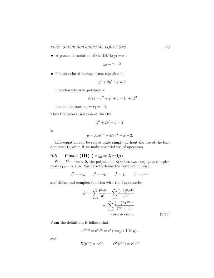
9.5 Cases (III) ( r1,2 = λ ± iµ)
When b2 − 4ac < 0, the polynomial φ(r) has two conjugate complexroots r1,2 = λ± iµ. We have to define the complex number,
i2 = −1; i3 = −i; i4 = 1; i5 = i, · · ·
and define and complex function with the Taylor series:
eix =∞∑
n=0
inxn
n!=
∞∑
n=0
(−1)nx2n
2n!
+i∞∑
n=0
(−1)nx2n+1
(2n + 1)!
= cosx + i sinx. (2.31)
From the definition, it follows that
ex+iy = exeiy = ex (cos y + i sin y) .
andD(erx) = rerx, Dn(erx) = rnerx
44 ORDINARY DIFFERENTIAL EQUATIONS AND LINEAR ALGEBRA
where r is a complex number. So that, the basic equalities are nowextended to the case with complex number r. Thus, we have the twocomplex solutions:
y1(x) = er1x = eλx(cosµx + i sinµx),
y2(x) = er2x = eλx(cosµx− i sinµx)
with a proper combination of these two solutions, one may derive tworeal solutions:
y1(x) =12[y1(x) + y2(x)] = eλx cosµx,
andy2(x) = −1
2i[y1(x)− y2(x)] = eλx sinµx
and the general solution:
y(x) = eλx(A cosµx + B sinµx).
10. Finding a Particular Solution forInhomogeneous Equation
In this section we shall discuss the methods for producing a particularsolution of a special kind for the general linear DE.
10.1 The Method of Variation of ParametersThe method of Variation of parameters is for producing a particular
solution of a special kind for the general linear DE in normal form
L(y) = y(n) + a1(x)y(n−1) + · · ·+ an(x)y = b(x)
from a fundamental set {y1, y2, . . . , yn} of solutions of the associatedhomogeneous equation.
In this method we try for a solution of the form
yP = C1(x)y1 + C2(x)y2 + · · ·+ Cn(x)yn.
Theny′P = C1(x)y′1 + C2(x)y′2 + · · ·+ Cn(x)y′n
+C ′1(x)y1 + C ′
2(x)y2 + · · ·+ C ′n(x)yn
and we impose the condition
C ′1(x)y1 + C ′
2(x)y2 + · · ·+ C ′n(x)yn = 0.
FIRST ORDER DIFFERENTIAL EQUATIONS 45
Theny′P = C1(x)y′1 + C2(x)y′2 + · · ·+ Cn(x)y′n
and hence
y′′P = C1(x)y′′1 + C2(x)y′′2 + · · ·+ Cn(x)y′′n+C ′
1(x)y′1 + C ′2(x)y′2 + · · ·+ C ′
n(x)y′n.
Again we impose the condition
C ′1(x)y′1 + C ′
2(x)y′2 + · · ·+ C ′n(x)y′n = 0
so thaty′′P = C1(x)y′′1 + C2(x)y′′2 + · · ·+ Cn(x)y′n.
We do this for the first n− 1 derivatives of y, so that
for 1 ≤ k ≤ n− 1
y(k)P = C1(x)y(k)
1 + C2(x)y(k)2 + · · ·Cn(x)y(k)
n ,
C ′1(x)y(k−1)
1 + C ′2(x)y(k−1)
2 + · · ·+ C ′n(x)y(k−1)
n = 0.
Now substituting yP , y′P , . . . , y(n−1)P in L(y) = b(x) we get
C1(x)L(y1) + C2(x)L(y2) + · · ·+ Cn(x)L(yn)
+C ′1(x)y(n−1)
1 + C ′2(x)y(n−1)
2 + · · ·+ C ′n(x)y(n−1)
n
= b(x).
But L(yi) = 0 for 1 ≤ k ≤ n so that
C ′1(x)y(n−1)
1 + C ′2(x)y(n−1)
2 + · · ·+ C ′n(x)y(n−1)
n = b(x).
We thus obtain the system of n linear equations for{C ′
1(x), . . . , C ′n(x)
}.
C ′1(x)y1 + C ′
2(x)y2 + · · ·+ C ′n(x)yn = 0,
C ′1(x)y′1 + C ′
2(x)y′2 + · · ·+ C ′n(x)y′n = 0,
...
C ′1(x)y(n−1)
1 + C ′2(x)y(n−1)
2 + · · ·+ C ′n(x)y(n−1)
n = b(x).
46 ORDINARY DIFFERENTIAL EQUATIONS AND LINEAR ALGEBRA
One can solve linear algebraic system by Cramer’s rule. Suppose that
(A)~x = ~b,
where
(A) =(~a1,~a2, · · · ,~an
)
~ai = [ai1, ai2, · · · , ain]T
~x = [x1, x2, · · · , xn]T
~b = [b1, b2, · · · , bn]T
Then we have the solution:
xj =det
(~a1,···,~aj−1,~b,~aj+1,···,~an
)
det
(~a1,···,~aj−1,~aj ,~aj+1,···,~an
) ,
n = 1, 2, · · · .
For our case, we have
~ai = [yi, y′i, · · · , yn−1
i ]T = ~yi, (i = 1, 2, · · ·)
~b = [0, 0, · · · , b(x)]T
hence, we solve
C ′j(x) =
det
(~y1,···,~yj−1,~b,~yj+1,···,~yn
)
det
(~y1,···,~yj−1,~yj ,~yj+1,···,~yn
) ,
(n = 1, 2, · · ·).Note that we can write
det(~y1, · · · , ~yj−1, ~yj , ~yj+1, · · · , ~yn
)= W (y1, y2, . . . yn),
where W (y1, y2, . . . yn) is the Wronskian. Moreover, in terms of thecofactor expansion theory, we can expand the determinant
det(~y1, · · · , ~yj−1,~b, ~yj+1, · · · , ~yn
)
along the column j. Since ~b only has one non-zero element, it followsthat
det(~y1, · · · , ~yj−1,~b, ~yj+1, · · · , ~yn
)
= (−1)n+jb(x)Wi.
FIRST ORDER DIFFERENTIAL EQUATIONS 47
Here we have use the notation:
Wi = W (y1, · · · , yj−1, yj , jj+1, · · · , yn),
where the yi means that yi is omitted from the Wronskian W .
Thus, we finally obtain we find
C ′i(x) = (−1)n+ib(t)
Wi
Wdt
and, after integration,
Ci(x) =∫ x
x0
(−1)n+ib(t)Wi
Wdt.
Note that the particular solution yP found in this way satisfies
yP (x0) = y′P (x0) = · · · = y(n−1)P = 0.
The point x0 is any point in the interval of continuity of the ai(x) andb(x). Note that yP is a linear function of the function b(x).
Example 2. Find the general solution of y′′ + y = 1/x on x > 0.The general solution of y′′ + y = 0 is
y = c1 cos(x) + c2 sin(x).
Using variation of parameters with
y1 = cos(x), y2 = sin(x), b(x) = 1/x
and x0 = 1, we have
W = 1, W1 = sin(x), W2 = cos(x)
and we obtain the particular solution
yp = C1(x) cos(x) + C2(x) sin(x)
whereC1(x) = −
∫ x
1
sin(t)t
dt, C2(x) =∫ x
1
cos(t)t
dt.
The general solution of y′′ + y = 1/x on x > 0 is therefore
y = c1 cos(x) + c2 sin(x)
−(∫ x
1sin(t)
t dt)
cos(x) +(∫ x
1cos(t)
t dt)
sin(x).
48 ORDINARY DIFFERENTIAL EQUATIONS AND LINEAR ALGEBRA
When applicable, the annihilator method is easier as one can see fromthe DE
y′′ + y = ex.
With(D − 1)ex = 0.
it is immediate that yp = ex/2 is a particular solution while variation ofparameters gives
yp = −(∫ x
0et sin(t)dt
)cos(x)
+(∫ x
0et cos(t)dt
)sin(x).
(2.32)
The integrals can be evaluated using integration by parts:∫ x
0et cos(t)dt = ex cos(x)− 1 +
∫ x
0et sin(t)dt
= ex cos(x) + ex sin(x)− 1
−∫ x
0et cos(t)dt
which gives∫ x
0et cos(t)dt =
[ex cos(x) + ex sin(x)− 1
]/2
∫ x
0et sin(t)dt = ex sin(x)
−∫ x
0et cos(t)dt
=[ex sin(x)− ex cos(x) + 1
]/2
so that after simplification
yp = ex/2− cos(x)/2− sin(x)/2.
10.2 Reduction of OrderIf y1 is a non-zero solution of a homogeneous linear n-th order DE
L[y] = 0, one can always find a new solution of the form
y = C(x)y1
for the inhomogeneous DE L[y] = b(x), where C ′(x) satisfies a homoge-neous linear DE of order n− 1. Since we can choose C ′(x) 6= 0, the new
FIRST ORDER DIFFERENTIAL EQUATIONS 49
solution y2 = C(x)y1 that we find in this way is not a scalar multiple ofy1.
In particular for n = 2, we obtain a fundamental set of solutions y1, y2.Let us prove this for the second order DE
p0(x)y′′ + p1(x)y′ + p2(x)y = 0.
If y1 is a non-zero solution we try for a solution of the form
y = C(x)y1.
Substituting y = C(x)y1 in the above we get
p0(x)(C ′′(x)y1 + 2C ′(x)y′1 + C(x)y′′1
)
+p1(x)(C ′(x)y1 + C(x)y′1
)+ p2(x)C(x)y1 = 0.
Simplifying, we get
p0y1C′′(x) + (2p0y
′1 + p1y1)C ′(x) = 0
sincep0y
′′1 + p1y
′1 + p2y1 = 0.
This is a linear first order homogeneous DE for C ′(x). Note that to solveit we must work on an interval where
y1(x) 6= 0.
However, the solution found can always be extended to the places wherey1(x) = 0 in a unique way by the fundamental theorem.
The above procedure can also be used to find a particularsolution of the non-homogenous DE
p0(x)y′′ + p1(x)y′ + p2(x)y = q(x)
from a non-zero solution of
p0(x)y′′ + p1(x)y′ + p2(x)y = 0.
Example 4. Solve y′′ + xy′ − y = 0.
Here y = x is a solution so we try for a solution of the form y = C(x)x.Substituting in the given DE, we get
C ′′(x)x + 2C ′(x) + x(C ′(x)x + C(x))− C(x)x = 0
50 ORDINARY DIFFERENTIAL EQUATIONS AND LINEAR ALGEBRA
which simplifies to
xC ′′(x) + (x2 + 2)C ′(x) = 0.
Solving this linear DE for C ′(x), we get
C ′(x) = Ae−x2/2/x2
so thatC(x) = A
∫dx
x2ex2/2+ B
Hence the general solution of the given DE is
y = A1x + A2x
∫dx
x2ex2/2.
Example 5. Solve y′′ + xy′ − y = x3ex.
By the previous example, the general solution of the associated ho-mogeneous equation is
yH = A1x + A2x
∫dx
x2ex2/2.
Substituting yp = xC(x) in the given DE we get
C ′′(x) + (x + x/2)C ′(x) = x2ex.
Solving for C ′(x) we obtain
C ′(x) = 1
x2ex2/2
(A2 +
∫x4ex+x2/2dx
)
= A21
x2ex2/2+ H(x),
whereH(x) =
1x2ex2/2
∫x4ex+x2/2dx.
This gives
C(x) = A1 + A2
∫dx
x2ex2/2+
∫H(x)dx,
We can therefore take
yp = x
∫H(x)dx,
so that the general solution of the given DE is
y = A1x + A2x
∫dx
x2ex2/2+ yp(x) = yH(x) + yp(x).
FIRST ORDER DIFFERENTIAL EQUATIONS 51
11. Solutions for Equations with VariableCoefficients
In this section we shall give a few techniques for solving certain lineardifferential equations with non-constant coefficients. We will mainlyrestrict our attention to second order equations. However, the techniquescan be extended to higher order equations. The general second orderlinear DE is
p0(x)y′′ + p1(x)y′ + p2(x)y = q(x).
This equation is called a non-constant coefficient equation if at least oneof the functions pi is not a constant function.
11.1 Euler EquationsAn important example of a non-constant linear DE is Euler’s equation
L[y] = xny(n) + a1xn−1y(n−1) + · · ·+ any = 0,
where a1, a2, . . . an are constants.This equation has singularity at x = 0. The fundamental theorem
of existence and uniqueness of solution holds in the region x > 0 andx < 0, respectively. So one must solve the problem in the region x > 0,or x < 0 separately. We first consider the region x > 0.
We assume that the solution has the following form: y = y(x) = xr,where r is a constant to be determined. Then it follows that
xy′(x) = ry(x),x2y′′(x) = r(r − 1)y(x),
· · ·xny(n)(x) = r(r − 1) · · · (r − n + 1)y(x)
Substitute into equation, we have
L[y(x)] = φ(r)xr = 0, for all x ∈ (I),
whereφ(r) = r(r − 1) · · · (r − n + 1)
+r(r − 1) · · · (r − n + 2)a1 + · · ·+r(r − 1)an−2 + ran−1 + an
is called the characteristic polynomial. It is derived that if r = r0 isa root of φ(r), such that φ(r0) = 0, then y(x) = xr0 must be a solutionof the Euler equation.
To demonstrate better, let us consider the special case (n = 2):
L[y] = x2y′′ + axy′ + by = 0,
52 ORDINARY DIFFERENTIAL EQUATIONS AND LINEAR ALGEBRA
where a, b are constants. In this case, we have the characteristic poly-nomial φ(r) = r(r− 1) + ar + b = r2 + (a− 1)r + b, which in general hastwo roots r = (r1, r2). Accordingly, the equation has two solutions:
{y1(x) = xr1 ; y2(x) = xr2}.Similar to the problem for the equations with constant coefficients, thereare three cases to be discussed separately.
11.2 Cases (I) ( r1 6= r2)
When (a − 1)2 − 4b > 0, the polynomial φ(r) has two distinct realroots (r1 6= r2). In this case, the two solutions, y1(x); y2(x) are linearindependent. The general solution of the equation is:
y(x) = Ay1(x) + By2(x), (2.33)
where A,B are arbitrary constants.
11.3 Cases (II) ( r1 = r2 )When (a− 1)2 − 4b = 0, the polynomial φ(r) has a double root r1 =
r2 = 1−a2 . In this case, the solution
y1(x) = y2(x) = xr1 .
Thus, for the general solution, one may derive the second solution byusing the method of reduction of order.
Let us look for a solution of the form C(x)y1(x) with the undeterminedfunction C(x). By substituting the equation, we derive that
L[C(x)y1(x)
]= C(x)φ(r1)y1(x) + C ′′(x)x2y1(x)
+C ′(x)[2x2y′1(x) + axy1(x)
]= 0.
Noting thatφ(r1) = 0; 2r1 + a = 1,
we getxC ′′(x) + C ′(x) = 0
or C ′(x) = Ax , and
C(x) = A ln |x|+ B,
where A,B are arbitrary constants. Thus, the solution:
y(x) = (A ln |x|+ B)x1−a2 . (2.34)
is a two parameter family of solutions consisting of the linear combina-tions of the two solutions:
y1 = xr1 , y2 = xr1 ln |x|.
FIRST ORDER DIFFERENTIAL EQUATIONS 53
11.4 Cases (III) ( r1,2 = λ ± iµ)
When (a−1)2−4b < 0, the polynomial φ(r) has two conjugate complexroots r1,2 = λ± iµ. Thus, we have the two complex solutions:
y1(x) = xr1 = er1 ln |x|
= eλ ln |x|[ cos(µ ln |x|) + i sin(µ ln |x|)]= |x|λ[ cos(µ ln |x|) + i sin(µ ln |x|)],
y2(x) = xr2 = er2 ln |x|
= eλ ln |x|[ cos(µ ln |x|)− i sin(µ ln |x|)]= |x|λ[ cos(µ ln |x|)− i sin(µ ln |x|)].
With a proper combination of these two solutions, one may derive tworeal solutions:
y1(x) =12[y1(x) + y2(x)] = |x|λ cos(µ ln |x|),
andy2(x) = −1
2i[y1(x)− y2(x)] = |x|λ sin(µ ln |x|).
and the general solution:
|x|λ[A cos(µ ln |x|) + B sin(µ ln |x|)].
Example 1. Solve x2y′′ + xy′ + y = 0, (x > 0).
The characteristic polynomial for the equation is
φ(r) = r(r − 1) + r + 1 = r2 + 1.
whose roots are r1,2 = ±i. The general solution of DE is
y = A cos(lnx) + B sin(lnx).
Example 2. Solve x3y′′′ + 2x2y′′ + xy′ − y = 0, (x > 0).
This is a third order Euler equation. Its characteristic polynomial is
φ(r) = r(r − 1)(r − 2) + 2r(r − 1) + r − 1= (r − 1)[r(r − 2) + 2r + 1]= (r − 1)(r2 + 1).
whose roots are r1,2,3 = (1,±i). The general solution od DE:
y = c1x + c2 sin(ln |x|) + c3 cos(ln |x|).
54 ORDINARY DIFFERENTIAL EQUATIONS AND LINEAR ALGEBRA
11.5 (*)Exact EquationsThe DE p0(x)y′′ + p1(x)y′ + p2(x)y = q(x) is said to be exact if
p0(x)y′′ + p1(x)y′ + p2(x)y =d
dx(A(x)y′ + B(x)y).
In this case the given DE is reduced to solving the linear DE
A(x)y′ + B(x)y =∫
q(x)dx + C
a linear first order DE. The exactness condition can be expressed inoperator form as
p0D2 + p1D + p2 = D(AD + B).
Sinced
dx(A(x)y′ + B(x)y) = A(x)y′′ + (A′(x)
+B(x))y′ + B′(x)y,
the exactness condition holds if and only if A(x), B(x) satisfy
A(x) = p0(x), B(x) = p1(x)− p′0(x), B′(x) = p2(x).
Since the last condition holds if and only if
p′1(x)− p′′0(x) = p2(x),
we see that the given DE is exact if and only if
p′′0 − p′1 + p2 = 0
in which case
p0(x)y′′ + p1(x)y′ + p2(x)y =ddx [p0(x)y′ + (p1(x)− p′0(x))y].
Example 3. Solve the DE xy′′ + xy′ + y = x, (x > 0).
This is an exact equation since the given DE can be written
d
dx(xy′ + (x− 1)y) = x.
Integrating both sides, we get
xy′ + (x− 1)y = x2/2 + A
which is a linear DE. The solution of this DE is left as an exercise.
Chapter 3
LAPLACE TRANSFORMS
1. IntroductionWe begin our study of the Laplace Transform with a motivating ex-
ample: Solve the differential equation
y′′ + y = f(t) =
0, 0 ≤ t < 10,1, 10 ≤ t < 10 + 2π,0, 10 + 2π ≤ t.
with IC’s:
y(0) = 0, y′(0) = 0 (3.1)
Here, f(t) is piecewise continuous and any solution would alsohave y′′ piecewise continuous. To describe the motion of the ball
using techniques previously developed we have to divide the probleminto three parts:
(I) 0 ≤ t < 10;
(II) 10 ≤ t < 10 + 2π;
(III) 10 + 2π ≤ t.
(I). The initial value problem determining the motion in part I is
y′′ + y = 0, y(0) = y′(0) = 0.
The solution isy(t) = 0, 0 ≤ t < 10.
55
56 ORDINARY DIFFERENTIAL EQUATIONS AND LINEAR ALGEBRA
Taking limits as t → 10 from the left, we find
y(10) = y′(10) = 0.
(II). The initial value problem determining the motion in part II is
y′′ + y = 1, y(10) = y′(10) = 0.
The solution is
y(t) = 1− cos(t− 10), 10 ≤ t < 2π + 10.
Taking limits as t → 10 + 2π from the left, we get
y(10 + 2π) = y′(10 + 2π) = 0.
(III). The initial value problem for the last part is
y′′ + y = 0, y(10 + 2π) = y′(10 + 2π) = 0
which has the solution
y(t) = 0, 10 + 2π ≤ t < ∞.
Putting all this together, we have
y(t) =
0, 0 ≤ t < 10,1− cos(t− 10), 10 ≤ t < 10 + 2π,0, 10 + 2π ≤ t.
The function y(t) is continuous with continuous derivative
y′(t) =
0, 0 ≤ t < 10,sin(t− 10), 10 ≤ t < 10 + 2π,0, 10 + 2π ≤ t.
However the function y′(t) is not differentiable at t = 10 and t = 10+2π.In fact
y′′(t) =
0, 0 ≤ t < 10,cos(t− 10), 10 < t < 10 + 2π,0, 10 + 2π < t.
The left-hand and right-hand limits of y′′(t) at t = 10 are 0 and 1respectively. At t = 10 + 2π they are 1 and 0.
By a solution we mean any function y = y(t) satisfying the DE for thoset not equal to the points of discontinuity of f(t). In this case we have
LAPLACE TRANSFORMS 57
shown that a solution exists with y(t), y′(t) continuous. In the same way,one can show that in general such solutions exist using the fundamentaltheorem.
We now want to describe is an approach for doing such problems withouthaving to divide the problem into parts. Such an approach is theLaplace transform.
2. Laplace Transform2.1 Definition2.1.1 Piecewise Continuous Function
Let f(t) be a function defined for t ≥ 0. The function f(t) is said tobe piecewise continuous, if
(1) f(t) converges to a finite limit f(0+) as t → 0+
(2) for any c > 0, the left and right hand limits f(c−), f(c+) of f(t)at c exist and are finite.
(3) f(c−) = f(c+) = f(c) for every c > 0 except possibly a finite setof points or an infinite sequence of points converging to +∞.
Thus the only points of discontinuity of f(t) are jump discontinuities.The function is said to be normalized if f(c) = f(c+) for every c ≥ 0.
2.1.2 Laplace TransformThe Laplace transform F (s) = L{{(t)} of given function f(x) is the
function of a new variable s defined by
F (s) =∫ ∞
0e−stf(t)dt = lim
N→+∞
∫ N
0e−stf(t)dt, (3.2)
provided that the improper integral exists.
2.2 Existence of Laplace TransformFor the function of exponential order, its Laplace transform exists.
The function f(t) is said to be of exponential order, if there are con-stants a,M such that
|f(t)| ≤ Meat
for all t.
very large of class of functions is of exponential order. For instance,the solutions of constant coefficient homogeneous DE’s are all of ex-ponential order.
58 ORDINARY DIFFERENTIAL EQUATIONS AND LINEAR ALGEBRA
For a function f(t) of exponential order, the convergence of theimproper integral in (3.2) is guaranteed. In fact, from
∫ N
0|e−stf(t)|dt ≤ M
∫ N
0e−(s−a)tdt
= M
{1
s− a− e−(s−a)N
s− a
}(3.3)
which shows that the improper integral converges absolutely whens > a. It shows that |F (s)| < M
s−a as N →∞.
3. Basic Properties and Formulas ofLaplace Transform
3.1 Linearity of Laplace Transform
L{af(t) + bg(t)} = aL{f(t)}+ bL{g(t)}.
3.2 Laplace Transforms for f(t) = eat
The calculation (3.3) shows that
L{eat} =1
s− a
for s > a. Setting a = 0, we get L{1} = 1s for s > 0.
The above holds when f(t) is complex valued and a = λ+iµ, s = σ + iτare complex numbers. The integral exists in this case for σ > λ.
For example, this yields
L{eit} =1
s− i, L{e−it} =
1s + i
.
3.3 Laplace Transforms for f(t) = {sin(bt) andcos(bt)}
Using the linearity property of the Laplace transform
L{af(t) + bf(t)} = aL{f(t)}+ bL{g(t)},
by using
sin(t) = (eit − e−it)/2i,
cos(t) = (eit + e−it)/2,
LAPLACE TRANSFORMS 59
we findL{sin(bt)} =
12i
( 1s− bi
− 1s + bi
)=
b
s2 + b2,
andL{cos(bt)} =
12
( 1s− bi
+1
s + bi
)=
s
s2 + b2,
for s > 0.
3.4 Laplace Transforms for {eatf(t); f(bt)}From the definition of the Laplace transform, we derive the following
two identities after a change of variable.
L{eatf(t)}(s) = L{f(t)}(s− a) = F (s− a),
L{f(bt)}(s) = 1bL{f(t)}(s/b) = 1
bF (s/b).
Using the first of these formulas, we get
L{eat sin(bt)} = b(s−a)2+b2
,
L{eat cos(bt)} = s−a(s−a)2+b2
.
3.5 Laplace Transforms for {tnf(t)}From the definition of the Laplace transform,
F (s) = L{f(t)}(s) =∫ ∞
0e−stf(t)dt, (3.4)
by taking the derivative with respect to s inside the integral, we canderive:
L{tnf(t)}(s) = (−1)n dn
dsnL{f(t)}(s).
For n = 1, one can verify the formula directly by differentiating withrespect s on the definition of the Laplace transform, whereas the generalcase follows by induction.
For example, using this formula, we obtain using f(t) = 1
L{tn}(s) = (−1)n dn
dsn
1s
=n!
sn+1.
With f(t) = sin(t) and f(t) = cos(t) we get
L{t sin(bt)}(s) = − dds
b
s2 + b2=
2bs
(s2 + b2)2,
60 ORDINARY DIFFERENTIAL EQUATIONS AND LINEAR ALGEBRA
L{t cos(bt)}(s) = − dds
s
s2 + b2=
s2 − b2
(s2 + b2)2
=1
s2 + b2− 2b2
(s2 + b2)2.
3.6 Laplace Transforms for {f ′(t)}The following formula shows how to compute the Laplace transform
of f ′(t) in terms of the Laplace transform of f(t):
L{f ′(t)}(s) = sL{f(t)}(s)− f(0).
This follows from
L{f ′(t)}(s) =∫ ∞
0e−stf ′(t)dt
= e−stf(t)∣∣∣∞0
+ s
∫ ∞
0e−stf(t)dt
= s
∫ ∞
0e−stf(t)dt− f(0), (3.5)
since e−stf(t) converges to 0 as t → +∞ in the domain of definition ofthe Laplace transform of f(t). To ensure that the first integral is defined,we have to assume f ′(t) is piecewise continuous. Repeated applicationsof this formula give
L{f (n)(t)}(s) = snL{f(t)}(s)− sn−1f(0)
−sn−2f ′(0)− · · · − fn−1(0).
The following theorem is important for the application of the Laplacetransform to differential equations.
4. Inverse Laplace Transform4.1 Theorem:
If f(t), g(t) are normalized piecewise continuous functions of expo-nential order then
L{f(t)} = L{g(t)}implies
f = g.
LAPLACE TRANSFORMS 61
4.2 DefinitionIf F (s) is the Laplace of the normalized piecewise continuous func-
tion f(t) of exponential order then f(t) is called the inverse Laplacetransform of F (s). This is denoted by
f(t) = L−1{F (s)}.Note that the inverse Laplace transform is also linear. Using the Laplacetransforms we found for t sin(bt), t cos(bt) we find
L−1{
s
(s2 + b2)2
}=
12b
t sin(bt),
andL−1
{1
(s2 + b2)2
}=
12b3
sin(bt)− 12b2
t cos(bt).
5. Solve IVP of DE’s with Laplace TransformMethod
In this lecture we will, by using examples, show how to use Laplacetransforms in solving differential equations with constant coefficients.
5.1 Example 1Consider the initial value problem
y′′ + y′ + y = sin(t), y(0) = 1, y′(0) = −1.
Step 1Let Y (s) = L{y(t)}, we have
L{y′(t)} = sY (s)− y(0) = sY (s)− 1,
L{y′′(t)} = s2Y (s)− sy(0)− y′(0)
= s2Y (s)− s + 1.
Taking Laplace transforms of the DE, we get
(s2 + s + 1)Y (s)− s =1
s2 + 1.
Step 2Solving for Y (s), we get
Y (s) =s
s2 + s + 1+
1(s2 + s + 1)(s2 + 1)
.
62 ORDINARY DIFFERENTIAL EQUATIONS AND LINEAR ALGEBRA
Step 3Finding the inverse laplace transform.
y(t) = L−1{Y (s)} = L−1{
ss2+s+1
}
+L−1{
1(s2+s+1)(s2+1)
}.
Since
s
s2 + s + 1=
s
(s + 1/2)2 + 3/4
=s + 1/2
(s + 1/2)2 + (√
3/2)2
− 1√3
√3/2
(s + 1/2)2 + (√
3/2)2
we have
L−1{
s
s2 + s + 1
}= e−t/2 cos(
√3 t/2)
− 1√3e−t/2 sin(
√3 t/2). (3.6)
Using partial fractions we have
1(s2 + s + 1)(s2 + 1)
=As + B
s2 + s + 1+
Cs + D
s2 + 1.
Multiplying both sides by (s2 + 1)(s2 + s + 1) and collecting terms, wefind
1 = (A + C)s3 + (B + C + D)s2 + (A + C + D)s + B + D.
Equating coefficients, we get A+C = 0, B +C +D = 0, A+C +D = 0,B + D = 1,
from which we get A = B = 1, C = −1, D = 0, so that
L−1{
1(s2 + s + 1)(s2 + 1)
}= L−1
{s + 1
s2 + s + 1
}
−L−1{
s
s2 + 1
}.
LAPLACE TRANSFORMS 63
Since
L−1{
1s2 + s + 1
}=
2√3e−t/2 sin(
√3 t/2),
L−1{
s
s2 + 1
}= cos(t)
we obtainy(t) = 2e−t/2 cos(
√3 t/2)− cos(t).
5.2 Example 2As we have known, a higher order DE can be reduced to a system of
DE’s. Let us consider the system
dx
dt= −2x + y,
dy
dt= x− 2y
(3.7)
with the initial conditions x(0) = 1, y(0) = 2.
Step 1Taking Laplace transforms the system becomes
sX(s)− 1 = −2X(s) + Y (s),
sY (s)− 2 = X(s)− 2Y (s),(3.8)
where X(s) = L{x(t)}, Y (s) = L{y(t)}.
Step 2Solving for X(s), Y (s). The above linear system of equations can bewritten in the form:
(s + 2)X(s)− Y (s) = 1,
−X(s) + (s + 2)Y (s) = 2.(3.9)
The determinant of the coefficient matrix is
s2 + 4s + 3 = (s + 1)(s + 3).
Using Cramer’s rule we get
X(s) =s + 4
s2 + 4s + 3, Y (s) =
2s + 5s2 + 4s + 3
.
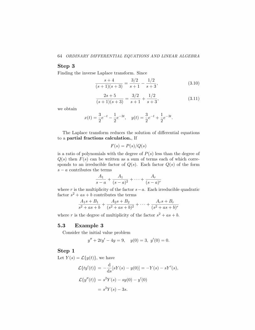
64 ORDINARY DIFFERENTIAL EQUATIONS AND LINEAR ALGEBRA
Step 3Finding the inverse Laplace transform. Since
s + 4(s + 1)(s + 3)
=3/2
s + 1− 1/2
s + 3, (3.10)
2s + 5(s + 1)(s + 3)
=3/2
s + 1+
1/2s + 3
, (3.11)
we obtain
x(t) =32e−t − 1
2e−3t, y(t) =
32e−t +
12e−3t.
The Laplace transform reduces the solution of differential equationsto a partial fractions calculation., If
F (s) = P (s)/Q(s)
is a ratio of polynomials with the degree of P (s) less than the degree ofQ(s) then F (s) can be written as a sum of terms each of which corre-sponds to an irreducible factor of Q(s). Each factor Q(s) of the forms− a contributes the terms
A1
s− a+
A1
(s− a)2+ · · ·+ Ar
(s− a)r
where r is the multiplicity of the factor s−a. Each irreducible quadraticfactor s2 + as + b contributes the terms
A1s + B1
s2 + as + b+
A2s + B2
(s2 + as + b)2+ · · ·+ Ars + Br
(s2 + as + b)r
where r is the degree of multiplicity of the factor s2 + as + b.
5.3 Example 3Consider the initial value problem
y′′ + 2ty′ − 4y = 9, y(0) = 3, y′(0) = 0.
Step 1Let Y (s) = L{y(t)}, we have
L{ty′(t)} = − dds
[sY (s)− y(0)] = −Y (s)− sY ′(s),
L{y′′(t)} = s2Y (s)− sy(0)− y′(0)
= s2Y (s)− 3s.
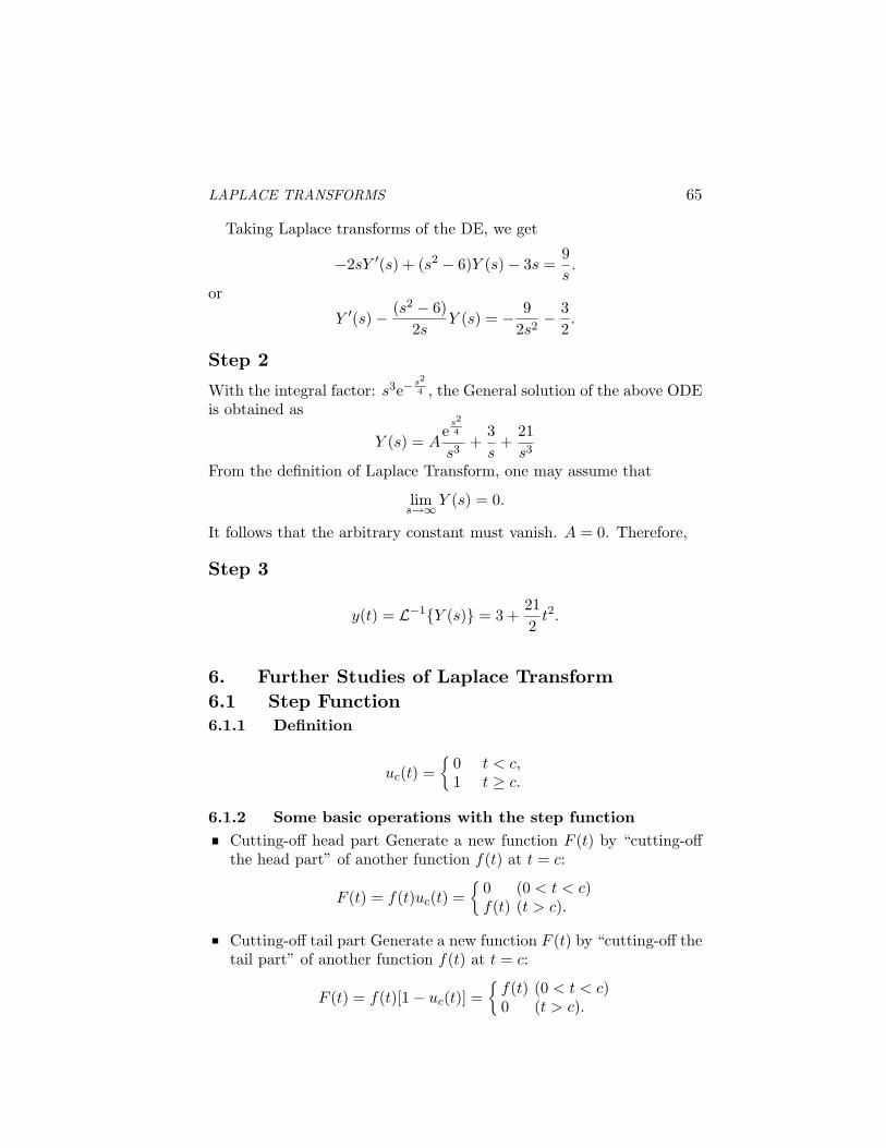
LAPLACE TRANSFORMS 65
Taking Laplace transforms of the DE, we get
−2sY ′(s) + (s2 − 6)Y (s)− 3s =9s.
or
Y ′(s)− (s2 − 6)2s
Y (s) = − 92s2
− 32.
Step 2
With the integral factor: s3e−s2
4 , the General solution of the above ODEis obtained as
Y (s) = Ae
s2
4
s3+
3s
+21s3
From the definition of Laplace Transform, one may assume that
lims→∞Y (s) = 0.
It follows that the arbitrary constant must vanish. A = 0. Therefore,
Step 3
y(t) = L−1{Y (s)} = 3 +212
t2.
6. Further Studies of Laplace Transform6.1 Step Function6.1.1 Definition
uc(t) ={
0 t < c,1 t ≥ c.
6.1.2 Some basic operations with the step functionCutting-off head part Generate a new function F (t) by “cutting-offthe head part” of another function f(t) at t = c:
F (t) = f(t)uc(t) ={
0 (0 < t < c)f(t) (t > c).
Cutting-off tail part Generate a new function F (t) by “cutting-off thetail part” of another function f(t) at t = c:
F (t) = f(t)[1− uc(t)] ={
f(t) (0 < t < c)0 (t > c).
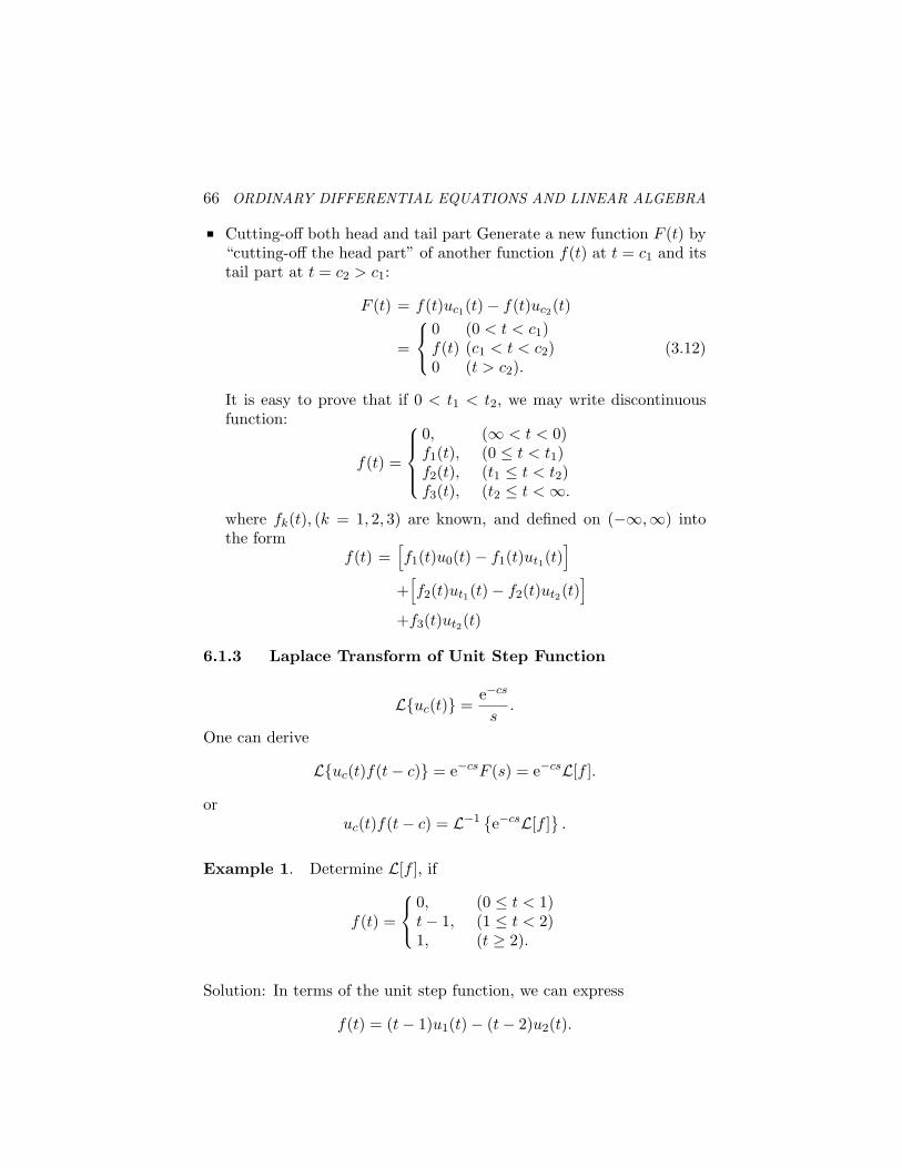
66 ORDINARY DIFFERENTIAL EQUATIONS AND LINEAR ALGEBRA
Cutting-off both head and tail part Generate a new function F (t) by“cutting-off the head part” of another function f(t) at t = c1 and itstail part at t = c2 > c1:
F (t) = f(t)uc1(t)− f(t)uc2(t)
=
0 (0 < t < c1)f(t) (c1 < t < c2)0 (t > c2).
(3.12)
It is easy to prove that if 0 < t1 < t2, we may write discontinuousfunction:
f(t) =
0, (∞ < t < 0)f1(t), (0 ≤ t < t1)f2(t), (t1 ≤ t < t2)f3(t), (t2 ≤ t < ∞.
where fk(t), (k = 1, 2, 3) are known, and defined on (−∞,∞) intothe form
f(t) =[f1(t)u0(t)− f1(t)ut1(t)
]
+[f2(t)ut1(t)− f2(t)ut2(t)
]
+f3(t)ut2(t)
6.1.3 Laplace Transform of Unit Step Function
L{uc(t)} =e−cs
s.
One can derive
L{uc(t)f(t− c)} = e−csF (s) = e−csL[f ].
oruc(t)f(t− c) = L−1 {
e−csL[f ]}
.
Example 1. Determine L[f ], if
f(t) =
0, (0 ≤ t < 1)t− 1, (1 ≤ t < 2)1, (t ≥ 2).
Solution: In terms of the unit step function, we can express
f(t) = (t− 1)u1(t)− (t− 2)u2(t).
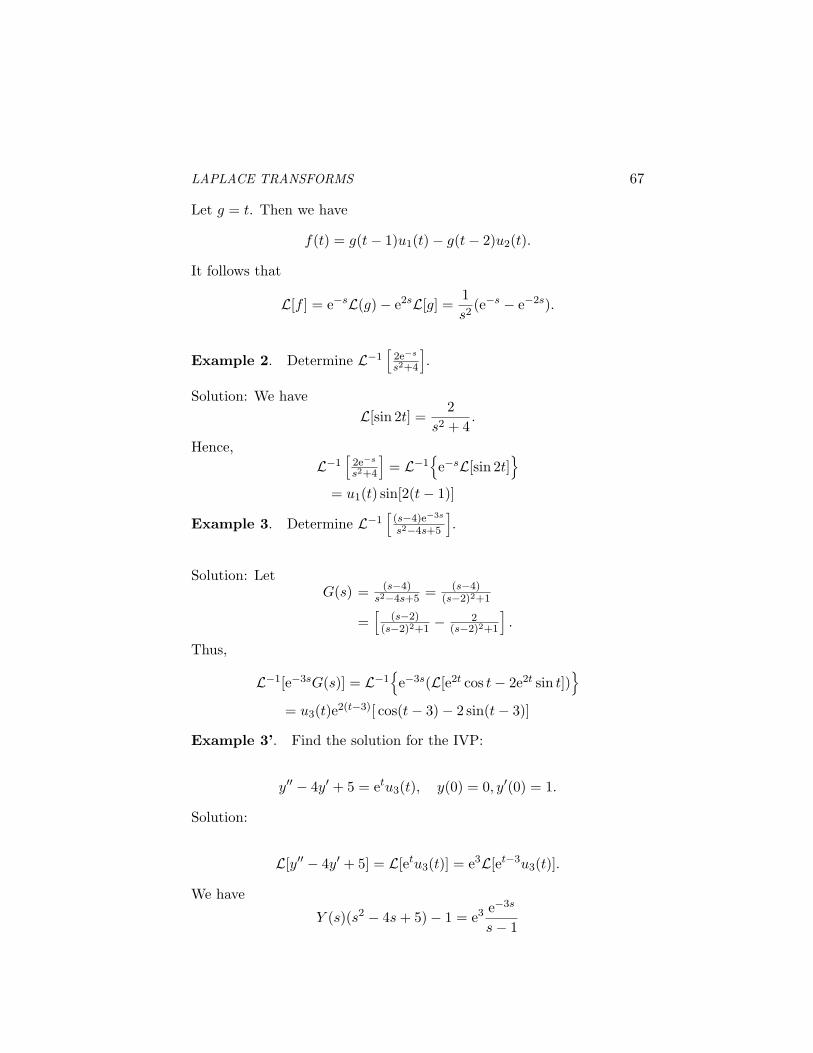
LAPLACE TRANSFORMS 67
Let g = t. Then we have
f(t) = g(t− 1)u1(t)− g(t− 2)u2(t).
It follows that
L[f ] = e−sL(g)− e2sL[g] =1s2
(e−s − e−2s).
Example 2. Determine L−1[
2e−s
s2+4
].
Solution: We haveL[sin 2t] =
2s2 + 4
.
Hence,L−1
[2e−s
s2+4
]= L−1
{e−sL[sin 2t]
}
= u1(t) sin[2(t− 1)]
Example 3. Determine L−1[
(s−4)e−3s
s2−4s+5
].
Solution: LetG(s) = (s−4)
s2−4s+5= (s−4)
(s−2)2+1
=[
(s−2)(s−2)2+1
− 2(s−2)2+1
].
Thus,
L−1[e−3sG(s)] = L−1{e−3s(L[e2t cos t− 2e2t sin t])
}
= u3(t)e2(t−3)[ cos(t− 3)− 2 sin(t− 3)]
Example 3’. Find the solution for the IVP:
y′′ − 4y′ + 5 = etu3(t), y(0) = 0, y′(0) = 1.
Solution:
L[y′′ − 4y′ + 5] = L[etu3(t)] = e3L[et−3u3(t)].
We have
Y (s)(s2 − 4s + 5)− 1 = e3 e−3s
s− 1
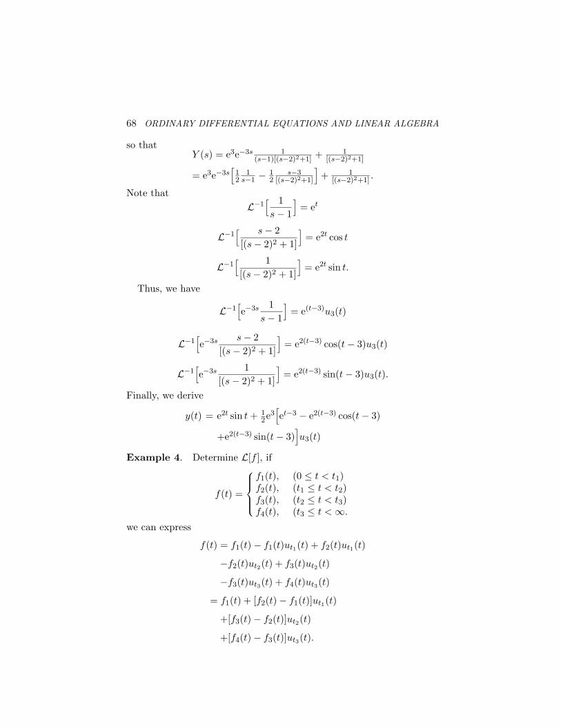
68 ORDINARY DIFFERENTIAL EQUATIONS AND LINEAR ALGEBRA
so thatY (s) = e3e−3s 1
(s−1)[(s−2)2+1]+ 1
[(s−2)2+1]
= e3e−3s[
12
1s−1 − 1
2s−3
[(s−2)2+1]
]+ 1
[(s−2)2+1].
Note thatL−1
[ 1s− 1
]= et
L−1[ s− 2[(s− 2)2 + 1]
]= e2t cos t
L−1[ 1[(s− 2)2 + 1]
]= e2t sin t.
Thus, we have
L−1[e−3s 1
s− 1
]= e(t−3)u3(t)
L−1[e−3s s− 2
[(s− 2)2 + 1]
]= e2(t−3) cos(t− 3)u3(t)
L−1[e−3s 1
[(s− 2)2 + 1]
]= e2(t−3) sin(t− 3)u3(t).
Finally, we derive
y(t) = e2t sin t + 12e3
[et−3 − e2(t−3) cos(t− 3)
+e2(t−3) sin(t− 3)]u3(t)
Example 4. Determine L[f ], if
f(t) =
f1(t), (0 ≤ t < t1)f2(t), (t1 ≤ t < t2)f3(t), (t2 ≤ t < t3)f4(t), (t3 ≤ t < ∞.
we can express
f(t) = f1(t)− f1(t)ut1(t) + f2(t)ut1(t)
−f2(t)ut2(t) + f3(t)ut2(t)
−f3(t)ut3(t) + f4(t)ut3(t)
= f1(t) + [f2(t)− f1(t)]ut1(t)
+[f3(t)− f2(t)]ut2(t)
+[f4(t)− f3(t)]ut3(t).
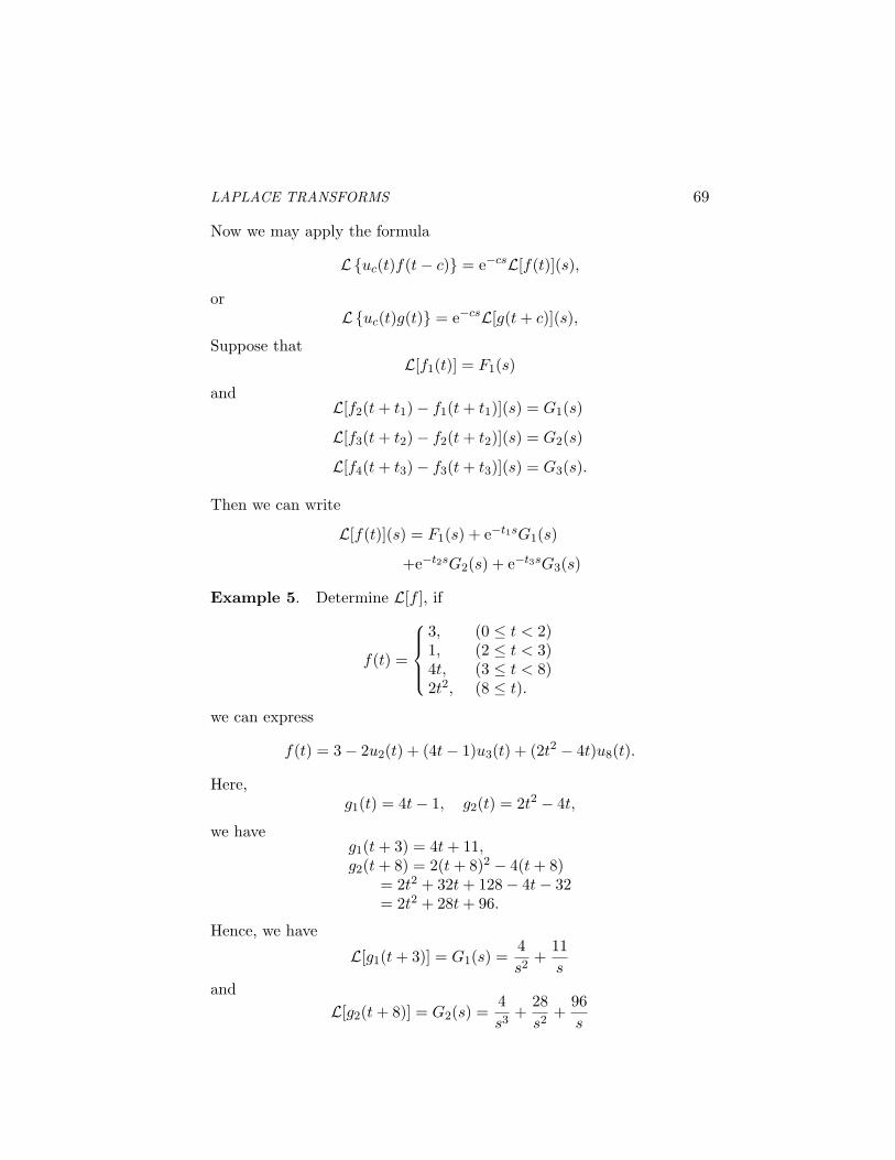
LAPLACE TRANSFORMS 69
Now we may apply the formula
L{uc(t)f(t− c)} = e−csL[f(t)](s),
orL{uc(t)g(t)} = e−csL[g(t + c)](s),
Suppose thatL[f1(t)] = F1(s)
andL[f2(t + t1)− f1(t + t1)](s) = G1(s)
L[f3(t + t2)− f2(t + t2)](s) = G2(s)
L[f4(t + t3)− f3(t + t3)](s) = G3(s).
Then we can write
L[f(t)](s) = F1(s) + e−t1sG1(s)
+e−t2sG2(s) + e−t3sG3(s)
Example 5. Determine L[f ], if
f(t) =
3, (0 ≤ t < 2)1, (2 ≤ t < 3)4t, (3 ≤ t < 8)2t2, (8 ≤ t).
we can express
f(t) = 3− 2u2(t) + (4t− 1)u3(t) + (2t2 − 4t)u8(t).
Here,g1(t) = 4t− 1, g2(t) = 2t2 − 4t,
we haveg1(t + 3) = 4t + 11,g2(t + 8) = 2(t + 8)2 − 4(t + 8)
= 2t2 + 32t + 128− 4t− 32= 2t2 + 28t + 96.
Hence, we have
L[g1(t + 3)] = G1(s) =4s2
+11s
andL[g2(t + 8)] = G2(s) =
4s3
+28s2
+96s
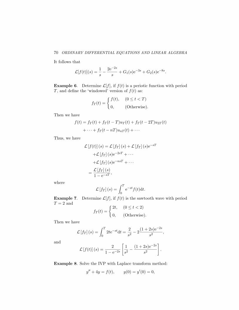
70 ORDINARY DIFFERENTIAL EQUATIONS AND LINEAR ALGEBRA
It follows that
L[f(t)](s) =1s− 2e−2s
s+ G1(s)e−3s + G2(s)e−8s.
Example 6. Determine L[f ], if f(t) is a periotic function with periodT , and define the ‘windowed’ version of f(t) as:
fT (t) =
{f(t), (0 ≤ t < T )
0, (Otherwise).
Then we have
f(t) = fT (t) + fT (t− T )uT (t) + fT (t− 2T )u2T (t)
+ · · ·+ fT (t− nT )unT (t) + · · ·Thus, we have
L [f(t)] (s) = L [fT ] (s) + L [fT ] (s)e−sT
+L [fT ] (s)e−2sT + · · ·+L [fT ] (s)e−nsT + · · ·
=L [fT ] (s)1− e−sT
,
where
L [fT ] (s) =∫ T
0e−stf(t)dt.
Example 7. Determine L[f ], if f(t) is the sawtooth wave with periodT = 2 and
fT (t) =
{2t, (0 ≤ t < 2)
0, (Otherwise).
Then we have
L [fT ] (s) =∫ T
02te−stdt =
2s2− 2
(1 + 2s)e−2s
s2,
and
L [f(t)] (s) =2
1− e−2s
[1s2− (1 + 2s)e−2s
s2
].
Example 8. Solve the IVP with Laplace transform method:
y′′ + 4y = f(t), y(0) = y′(0) = 0,
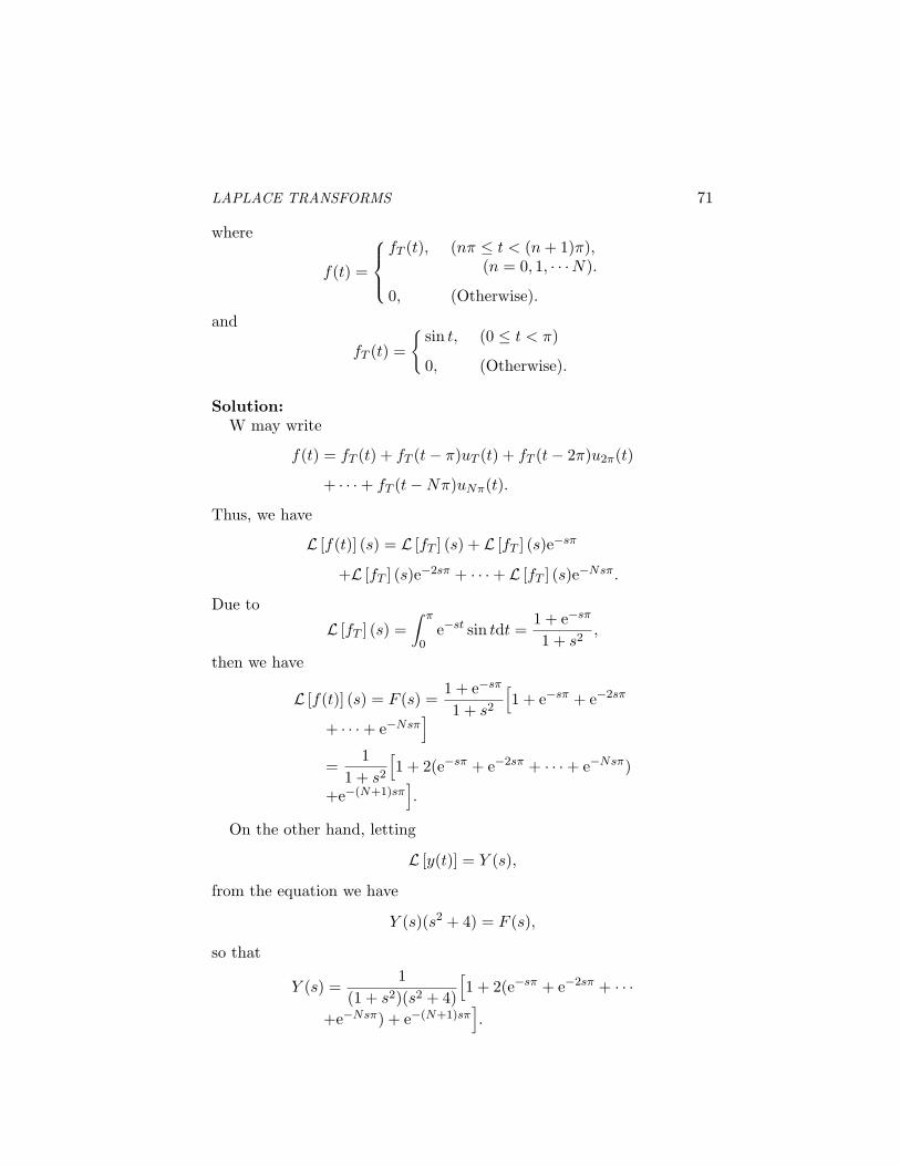
LAPLACE TRANSFORMS 71
where
f(t) =
fT (t), (nπ ≤ t < (n + 1)π),(n = 0, 1, · · ·N).
0, (Otherwise).
and
fT (t) =
{sin t, (0 ≤ t < π)
0, (Otherwise).
Solution:W may write
f(t) = fT (t) + fT (t− π)uT (t) + fT (t− 2π)u2π(t)
+ · · ·+ fT (t−Nπ)uNπ(t).
Thus, we have
L [f(t)] (s) = L [fT ] (s) + L [fT ] (s)e−sπ
+L [fT ] (s)e−2sπ + · · ·+ L [fT ] (s)e−Nsπ.
Due to
L [fT ] (s) =∫ π
0e−st sin tdt =
1 + e−sπ
1 + s2,
then we have
L [f(t)] (s) = F (s) =1 + e−sπ
1 + s2
[1 + e−sπ + e−2sπ
+ · · ·+ e−Nsπ]
=1
1 + s2
[1 + 2(e−sπ + e−2sπ + · · ·+ e−Nsπ)
+e−(N+1)sπ].
On the other hand, letting
L [y(t)] = Y (s),
from the equation we have
Y (s)(s2 + 4) = F (s),
so that
Y (s) =1
(1 + s2)(s2 + 4)
[1 + 2(e−sπ + e−2sπ + · · ·
+e−Nsπ) + e−(N+1)sπ].
72 ORDINARY DIFFERENTIAL EQUATIONS AND LINEAR ALGEBRA
LetH(s) =
1(1 + s2)(s2 + 4)
=13
[1
(1 + s2)− 1
(s2 + 4)
].
We haveh(t) = L−1 [H(s)] =
(13
sin t− 16
sin 2t
).
Therefore, we may derive
y(t) = L−1 [Y (s)] =(
13 sin t− 1
6 sin 2t)
+2uπ
[13 sin(t− π)− 1
6 sin 2(t− π)]
+2u2π
[13 sin(t− 2π)
−16 sin 2(t− 2π)
]+ · · ·
+2uNπ
[13 sin(t−Nπ)− 1
6 sin 2(t−Nπ)]
+u(N+1)π
[13 sin(t− (N + 1)π)
−16 sin 2(t− (N + 1)π)
]
ory(t) = L−1 [Y (s)] =
(13 sin t− 1
6 sin 2t)
+2uπ
[−1
3 sin t− 16 sin 2t
]
+2u2π
[13 sin t− 1
6 sin 2t]+ · · ·
+2uNπ
[13(−1)N sin t− 1
6 sin 2t]
+u(N+1)π
[13(−1)N+1 sin t− 1
6 sin 2t].
6.2 Impulse Function6.2.1 Definition
Let
dτ (t) ={ 1
2τ |t| < τ,0 |t| ≥ τ.
It follows thatI(τ) =
∫ ∞
−∞dτ (t)dt = 1.
Now, consider the limit,
δ(t) = limτ→0
dτ (t) ={
0 t 6= 0,∞ t = 0,
LAPLACE TRANSFORMS 73
which is called the Dirac δ-function. Evidently, the Dirac δ-functionhas the following properties:
1 ∫ ∞
−∞δ(t)dt = 1.
2 ∫ B
Aδ(t− c)dt =
{0 c ∈(A,B),1 c ∈ (A,B).
3 ∫ B
Aδ(t− c)f(t)dt =
{0 c ∈(A,B),f(c) c ∈ (A,B).
6.2.2 Laplace Transform of Impulse Function
L{δ(t− c)} ={
e−cs c > 0,0 c < 0.
One can derive
L{δ(t− c)f(t)} = e−csf(c), (c > 0).
Example 1. Solve the IVP:
y′′ + 4y′ + 13y = δ(t− π),
withy(0) = 2, y′(0) = 1.
Solution: Take the Laplace transform of both sides, and impose IC’s. Itfollows that
[s2Y − 2s− 1] + 4[sY − 2] + 13Y = e−πs
We haveY = e−πs+2s+9
s2+4s+13= e−πs+2s+9
(s+2)2+9
= e−πs
(s+2)2+9+ 2(s+2)
(s+2)2+9+ 5
(s+2)2+9.
Take the inverse of the Laplace transform on both sides. we derive
y = L−1{
e−πs
3 L[e−2t sin 3t]}
+2[e−2t cos 3t] + 53 [e−2t sin 3t]
= 13uπ(t)e−2(t−π) sin 3(t− π)
+2[e−2t cos 3t] + 53 [e−2t sin 3t].
74 ORDINARY DIFFERENTIAL EQUATIONS AND LINEAR ALGEBRA
6.3 Convolution Integral6.3.1 Theorem
GivenL{f(t)} = F (s), L{g(t)} = G(s),
one can deriveL−1{F (s) ·G(s)} = f(t) ∗ g(t)
= L−1{F (s)} ∗ L−1{G(s)}where
f(t) ∗ g(t) =∫ t
0f(t− τ)g(τ)dτ
is called the convolution integral.
Proof:
L{f ∗ g(t)} =∫ ∞
0e−st
{∫ t
0f(t− τ)g(τ)dτ
}dt
=∫ ∞
0
{∫ t
0e−stf(t− τ)g(τ)dτ
}dt.
However, it can be proven that
∫∞0
{∫ t0 e−stf(t− τ)g(τ)dτ
}dt
=∫∞0
{∫∞τ e−stf(t− τ)g(τ)dt
}dτ.
Now let u = t− τ . We get
L{f ∗ g(t)} =∫ ∞
0
{∫ ∞
0e−s(u+τ)f(u)g(τ)du
}dτ
= L{f(t)} · L{g(t)}
6.3.2 The properties of convolution integralf(t) ∗ g(t) = g(t) ∗ f(t).
[cf(t) + dg(t)] ∗ h(t) = c[f(t) ∗ h(t)] + d[g(t) ∗ h(t)].
1 ∗ g(t) 6= g(t)
0 ∗ g(t) = 0.
Example 1. Determine L−1[
G(s)(s−1)2+1
].
LAPLACE TRANSFORMS 75
Solution:
L−1[
G(s)(s−1)2+1
]= L−1[G(s)] ∗ L−1
[1
(s−1)2+1
]
= e−t sin t ∗ g(t).
Example 2. Solve the IVP:
y′′ + ω2y = f(t)
withy(0) = α, y′(0) = β.
Solution: Step #1: Taking Laplace transform of both sides, it follows
that[s2Y − αs− β] + ω2Y = F (s).
Step #2: We solve
Y (s) =F (s)
s2 + ω2+
αs
s2 + ω2+
β
s2 + ω2.
Step #3: Taking inverse Laplace transform of both sides, we obtain
y(t) = 1ω
∫ t0 sinω(t− τ)f(τ)dτ
+α cosωt + βω sinωt.

Chapter 4
SOLUTIONS OF SYSTEMS OF LINEARALGEBRAIC EQUATIONS
1. Introduction2. Introduction
The following chapters will devote the study of linear algebraicequations. A equation is generally written in the form, like
f(x) = 0.
It is called algebraic equation, if the function f(x) is polynomial,otherwise, called transcendental equation,
It is called Linear equation, if f(x) = a1x1 + a2x2 + · · · + a0,otherwise, called non-linear equation.
In this chapter, we are going to find the solution properties of a systemof (2× 3) linear algebraic equation, such as:
x1 + x2 − x3 = 1,
3x1 + 2x2 − 4x3 = 3. (4.1)
3. Solutions for general (m × n) System of LinearEquations
In general, a system of (m× n) equation is
a11x1 + a12x2 + · · ·+ a1nxn = b1,
a21x1 + a22x2 + · · ·+ a2nxn = b2,...
am1x1 + am2x2 + · · ·+ amnxn = bm.
77
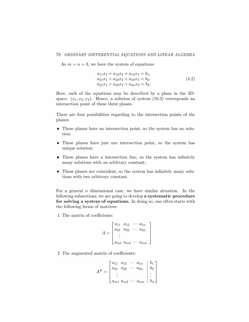
78 ORDINARY DIFFERENTIAL EQUATIONS AND LINEAR ALGEBRA
As m = n = 3, we have the system of equations:
a11x1 + a12x2 + a13x3 = b1,a21x1 + a22x2 + a23x3 = b2,a31x1 + a32x2 + a3nx3 = b3.
(4.2)
Here, each of the equations may be described by a plane in the 3D-space: (x1, x2, x3). Hence, a solution of system (10.3) corresponds anintersection point of these three planes.
There are four possibilities regarding to the intersection points of theplanes:
These planes have no intersection point, so the system has no solu-tion;
These planes have just one intersection point, so the system hasunique solution;
These planes have a intersection line, so the system has infinitelymany solutions with an arbitrary constant;
These planes are coincident, so the system has infinitely many solu-tions with two arbitrary constant.
For a general n dimensional case, we have similar situation. In thefollowing subsections, we are going to develop a systematic procedurefor solving a system of equations. In doing so, one often starts withthe following forms of matrices:
1 The matrix of coefficients:
A =
a11 a12 · · · a1n
a21 a22 · · · a2n...
am1 am2 · · · amn
2 The augmented matrix of coefficients:
A# =
a11 a12 · · · a1n
a21 a22 · · · a2n...
am1 am2 · · · amn
∣∣∣∣∣∣∣∣∣
b1
b2...bn
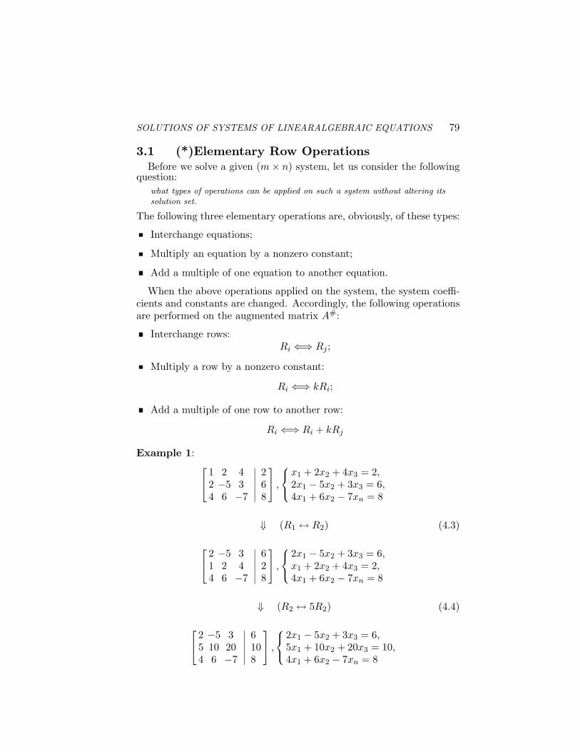
SOLUTIONS OF SYSTEMS OF LINEARALGEBRAIC EQUATIONS 79
3.1 (*)Elementary Row OperationsBefore we solve a given (m× n) system, let us consider the following
question:what types of operations can be applied on such a system without altering itssolution set.
The following three elementary operations are, obviously, of these types:
Interchange equations;
Multiply an equation by a nonzero constant;
Add a multiple of one equation to another equation.
When the above operations applied on the system, the system coeffi-cients and constants are changed. Accordingly, the following operationsare performed on the augmented matrix A#:
Interchange rows:Ri ⇐⇒ Rj ;
Multiply a row by a nonzero constant:
Ri ⇐⇒ kRi;
Add a multiple of one row to another row:
Ri ⇐⇒ Ri + kRj
Example 1:
1 2 42 −5 34 6 −7
∣∣∣∣∣∣
268
,
x1 + 2x2 + 4x3 = 2,2x1 − 5x2 + 3x3 = 6,4x1 + 6x2 − 7xn = 8
⇓ (R1 ↔ R2) (4.3)
2 −5 31 2 44 6 −7
∣∣∣∣∣∣
628
,
2x1 − 5x2 + 3x3 = 6,x1 + 2x2 + 4x3 = 2,4x1 + 6x2 − 7xn = 8
⇓ (R2 ↔ 5R2) (4.4)
2 −5 35 10 204 6 −7
∣∣∣∣∣∣
6108
,
2x1 − 5x2 + 3x3 = 6,5x1 + 10x2 + 20x3 = 10,4x1 + 6x2 − 7xn = 8
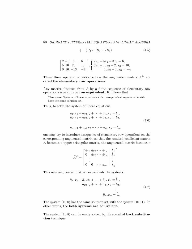
80 ORDINARY DIFFERENTIAL EQUATIONS AND LINEAR ALGEBRA
⇓ (R3 ↔ R3 − 2R1) (4.5)
2 −5 35 10 200 16 −13
∣∣∣∣∣∣
610−4
,
2x1 − 5x2 + 3x3 = 6,5x1 + 10x2 + 20x3 = 10,
16x2 − 13x3 = −4
These three operations performed on the augmented matrix A# arecalled the elementary row operations.
Any matrix obtained from A by a finite sequence of elementary rowoperations is said to be row-equivalent. It follows that
Theorem: Systems of linear equations with row-equivalent augmented matrixhave the same solution set.
Thus, to solve the system of linear equations,
a11x1 + a12x2 + · · ·+ a1nxn = b1,a21x1 + a22x2 + · · ·+ a2nxn = b2,
...an1x1 + an2x2 + · · ·+ annxn = bn,
(4.6)
one may try to introduce a sequence of elementary row operations on thecorresponding augmented matrix, so that the resulted coefficient matrixA becomes a upper triangular matrix, the augmented matrix becomes :
A# =
a11 a12 · · · a1n
0 a22 · · · a2n...
0 0 · · · ann
∣∣∣∣∣∣∣∣∣
b1
b2...bn
This new augmented matrix corresponds the systems:
a11x1 + a12x2 + · · ·+ a1nxn = b1,
a22x2 + · · ·+ a2nxn = b2,...
annxn = bn
(4.7)
The system (10.8) has the same solution set with the system (10.11). Inother words, the both systems are equivalent.
The system (10.8) can be easily solved by the so-called back substitu-tion technique.
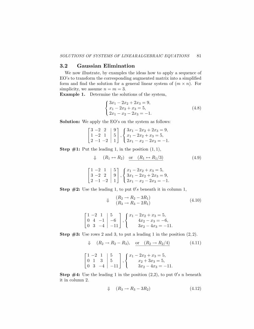
SOLUTIONS OF SYSTEMS OF LINEARALGEBRAIC EQUATIONS 81
3.2 Gaussian EliminationWe now illustrate, by examples the ideas how to apply a sequence of
EO’s to transform the corresponding augmented matrix into a simplifiedform and find the solution for a general linear system of (m × n). Forsimplicity, we assume n = m = 3.Example 1. Determine the solutions of the system,
3x1 − 2x2 + 2x3 = 9,x1 − 2x2 + x3 = 5,2x1 − x2 − 2x3 = −1.
(4.8)
Solution: We apply the EO’s on the system as follows:
3 −2 21 −2 12 −1 −2
∣∣∣∣∣∣
951
,
3x1 − 2x2 + 2x3 = 9,x1 − 2x2 + x3 = 5,2x1 − x2 − 2x3 = −1.
Step #1: Put the leading 1, in the position (1, 1),
⇓ (R1 ↔ R2) or (R1 ↔ R1/3) (4.9)
1 −2 13 −2 22 −1 −2
∣∣∣∣∣∣
591
,
x1 − 2x2 + x3 = 5,3x1 − 2x2 + 2x3 = 9,2x1 − x2 − 2x3 = −1.
Step #2: Use the leading 1, to put 0′s beneath it in column 1,
⇓ (R2 → R2 − 3R1)(R3 → R3 − 2R1)
(4.10)
1 −2 10 4 −10 3 −4
∣∣∣∣∣∣
5−6−11
,
x1 − 2x2 + x3 = 5,4x2 − x3 = −6,3x2 − 4x3 = −11.
Step #3: Use rows 2 and 3, to put a leading 1 in the position (2, 2).
⇓ (R2 → R2 −R3), or (R2 → R2/4) (4.11)
1 −2 10 1 30 3 −4
∣∣∣∣∣∣
55−11
,
x1 − 2x2 + x3 = 5,x2 + 3x3 = 5,3x2 − 4x3 = −11.
Step #4: Use the leading 1 in the position (2,2), to put 0′s n beneathit in column 2.
⇓ (R3 → R3 − 3R2) (4.12)
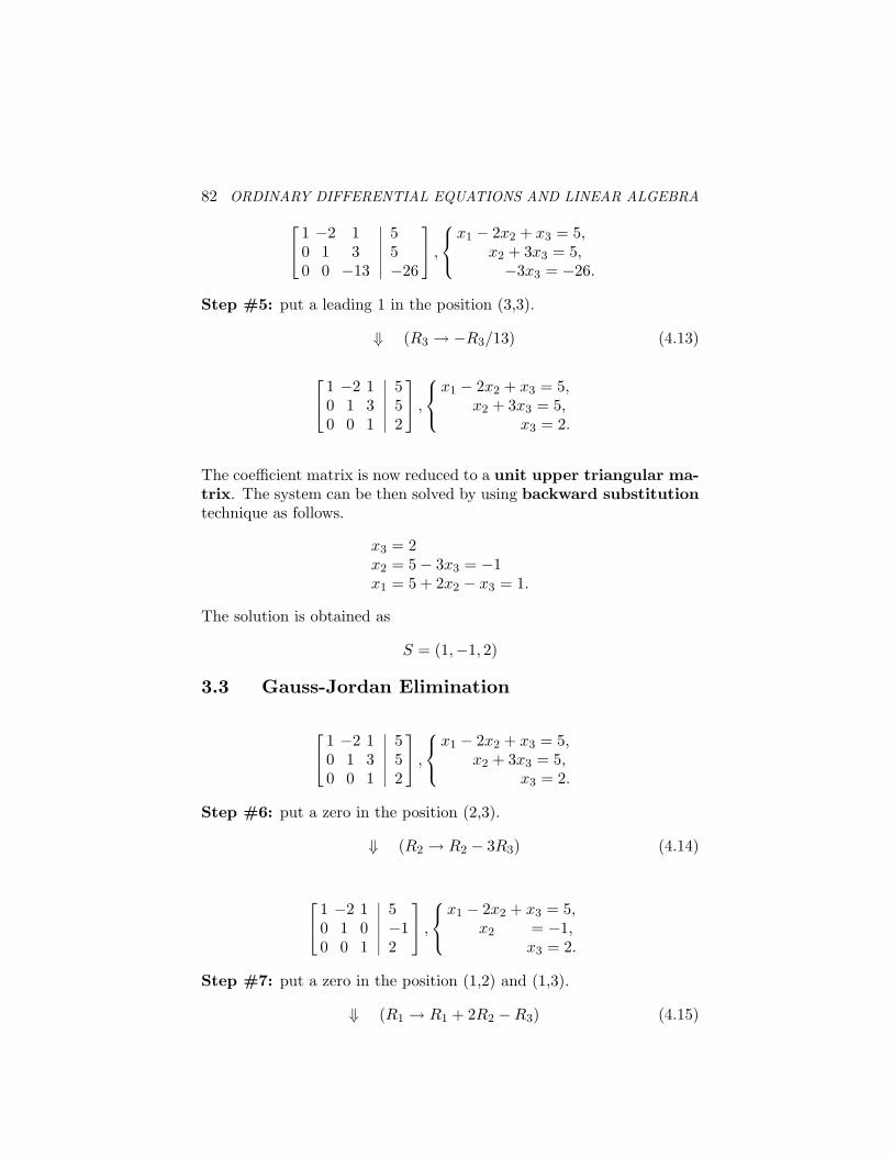
82 ORDINARY DIFFERENTIAL EQUATIONS AND LINEAR ALGEBRA
1 −2 10 1 30 0 −13
∣∣∣∣∣∣
55−26
,
x1 − 2x2 + x3 = 5,x2 + 3x3 = 5,−3x3 = −26.
Step #5: put a leading 1 in the position (3,3).
⇓ (R3 → −R3/13) (4.13)
1 −2 10 1 30 0 1
∣∣∣∣∣∣
552
,
x1 − 2x2 + x3 = 5,x2 + 3x3 = 5,
x3 = 2.
The coefficient matrix is now reduced to a unit upper triangular ma-trix. The system can be then solved by using backward substitutiontechnique as follows.
x3 = 2x2 = 5− 3x3 = −1x1 = 5 + 2x2 − x3 = 1.
The solution is obtained as
S = (1,−1, 2)
3.3 Gauss-Jordan Elimination
1 −2 10 1 30 0 1
∣∣∣∣∣∣
552
,
x1 − 2x2 + x3 = 5,x2 + 3x3 = 5,
x3 = 2.
Step #6: put a zero in the position (2,3).
⇓ (R2 → R2 − 3R3) (4.14)
1 −2 10 1 00 0 1
∣∣∣∣∣∣
5−12
,
x1 − 2x2 + x3 = 5,x2 = −1,
x3 = 2.
Step #7: put a zero in the position (1,2) and (1,3).
⇓ (R1 → R1 + 2R2 −R3) (4.15)
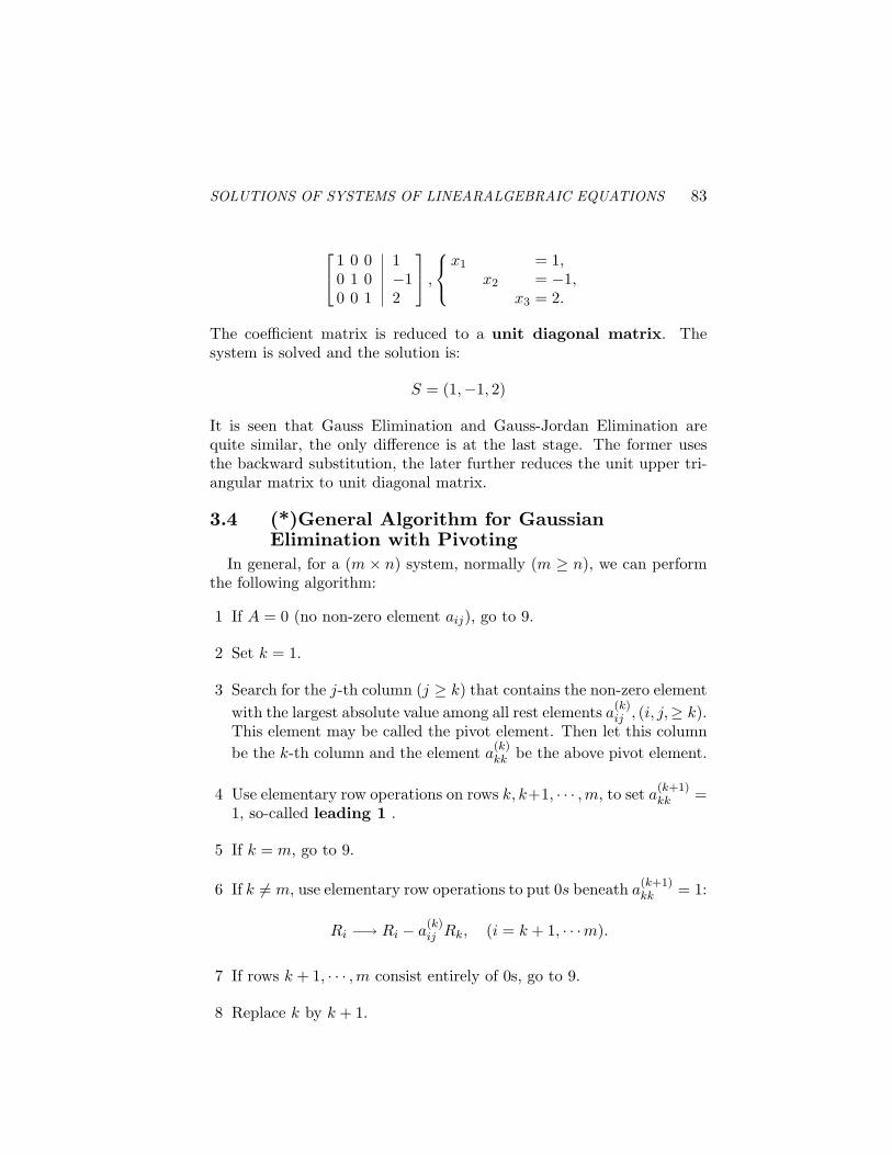
SOLUTIONS OF SYSTEMS OF LINEARALGEBRAIC EQUATIONS 83
1 0 00 1 00 0 1
∣∣∣∣∣∣
1−12
,
x1 = 1,x2 = −1,
x3 = 2.
The coefficient matrix is reduced to a unit diagonal matrix. Thesystem is solved and the solution is:
S = (1,−1, 2)
It is seen that Gauss Elimination and Gauss-Jordan Elimination arequite similar, the only difference is at the last stage. The former usesthe backward substitution, the later further reduces the unit upper tri-angular matrix to unit diagonal matrix.
3.4 (*)General Algorithm for GaussianElimination with Pivoting
In general, for a (m× n) system, normally (m ≥ n), we can performthe following algorithm:
1 If A = 0 (no non-zero element aij), go to 9.
2 Set k = 1.
3 Search for the j-th column (j ≥ k) that contains the non-zero elementwith the largest absolute value among all rest elements a
(k)ij , (i, j,≥ k).
This element may be called the pivot element. Then let this columnbe the k-th column and the element a
(k)kk be the above pivot element.
4 Use elementary row operations on rows k, k+1, · · · , m, to set a(k+1)kk =
1, so-called leading 1 .
5 If k = m, go to 9.
6 If k 6= m, use elementary row operations to put 0s beneath a(k+1)kk = 1:
Ri −→ Ri − a(k)ij Rk, (i = k + 1, · · ·m).
7 If rows k + 1, · · · , m consist entirely of 0s, go to 9.
8 Replace k by k + 1.
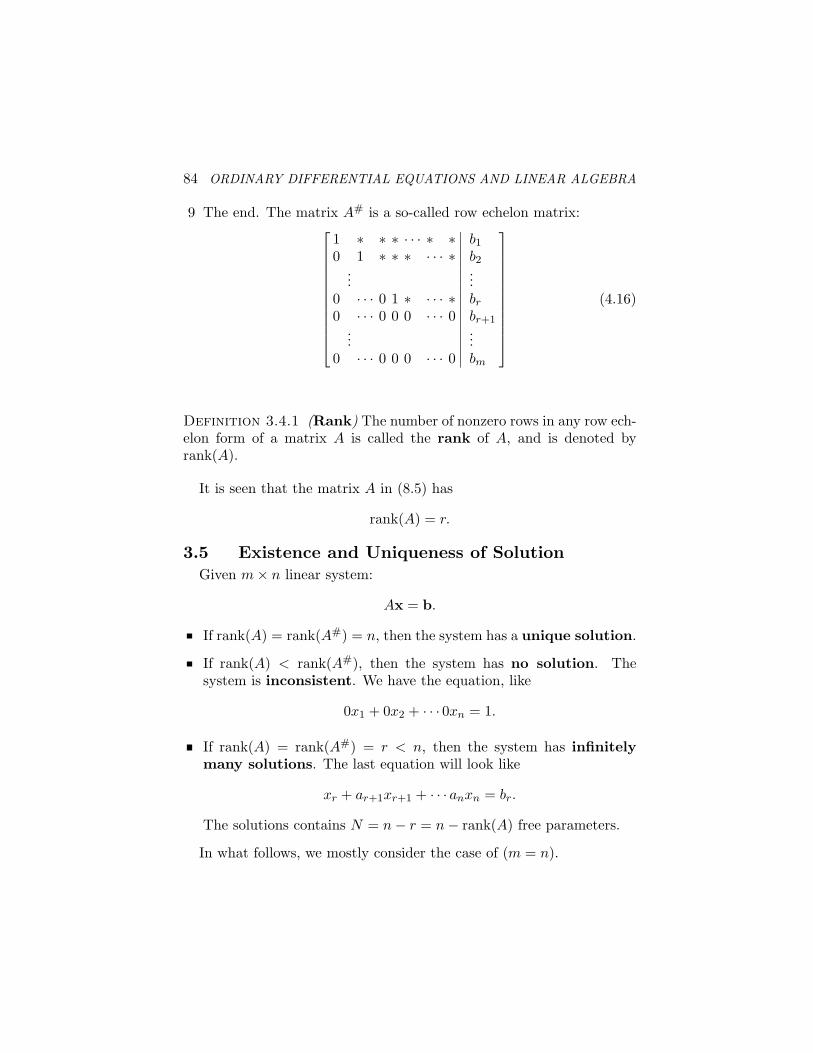
84 ORDINARY DIFFERENTIAL EQUATIONS AND LINEAR ALGEBRA
9 The end. The matrix A# is a so-called row echelon matrix:
1 ∗ ∗ ∗ · · · ∗ ∗0 1 ∗ ∗ ∗ · · · ∗
...0 · · · 0 1 ∗ · · · ∗0 · · · 0 0 0 · · · 0
...0 · · · 0 0 0 · · · 0
∣∣∣∣∣∣∣∣∣∣∣∣∣∣∣∣∣
b1
b2...br
br+1...bm
(4.16)
Definition 3.4.1 (Rank) The number of nonzero rows in any row ech-elon form of a matrix A is called the rank of A, and is denoted byrank(A).
It is seen that the matrix A in (8.5) has
rank(A) = r.
3.5 Existence and Uniqueness of SolutionGiven m× n linear system:
Ax = b.
If rank(A) = rank(A#) = n, then the system has a unique solution.
If rank(A) < rank(A#), then the system has no solution. Thesystem is inconsistent. We have the equation, like
0x1 + 0x2 + · · · 0xn = 1.
If rank(A) = rank(A#) = r < n, then the system has infinitelymany solutions. The last equation will look like
xr + ar+1xr+1 + · · · anxn = br.
The solutions contains N = n− r = n− rank(A) free parameters.
In what follows, we mostly consider the case of (m = n).
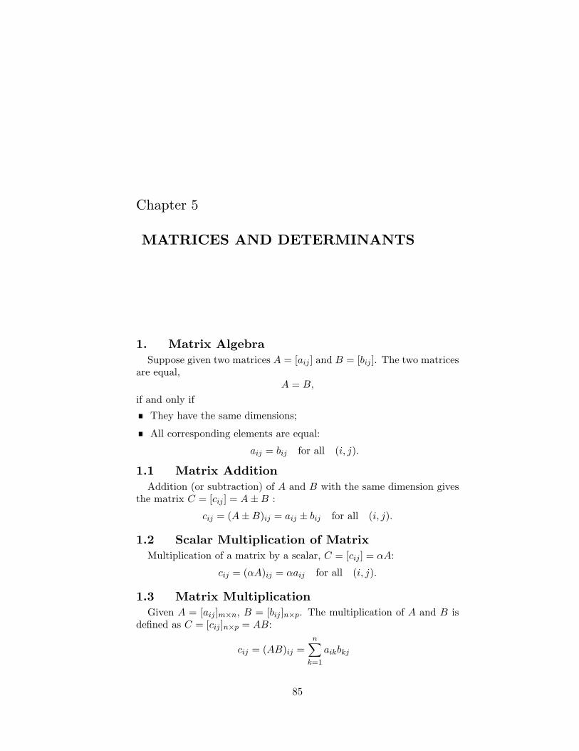
Chapter 5
MATRICES AND DETERMINANTS
1. Matrix AlgebraSuppose given two matrices A = [aij ] and B = [bij ]. The two matrices
are equal,A = B,
if and only if
They have the same dimensions;
All corresponding elements are equal:
aij = bij for all (i, j).
1.1 Matrix AdditionAddition (or subtraction) of A and B with the same dimension gives
the matrix C = [cij ] = A±B :
cij = (A±B)ij = aij ± bij for all (i, j).
1.2 Scalar Multiplication of MatrixMultiplication of a matrix by a scalar, C = [cij ] = αA:
cij = (αA)ij = αaij for all (i, j).
1.3 Matrix MultiplicationGiven A = [aij ]m×n, B = [bij ]n×p. The multiplication of A and B is
defined as C = [cij ]n×p = AB:
cij = (AB)ij =n∑
k=1
aikbkj
85
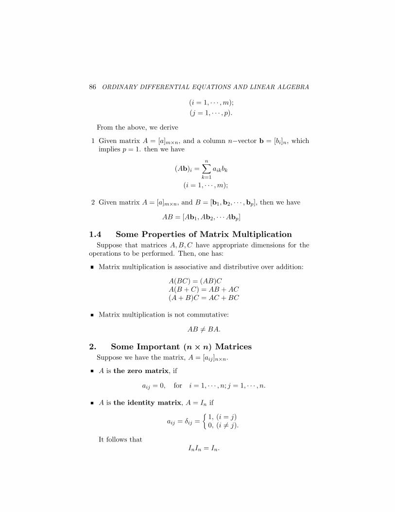
86 ORDINARY DIFFERENTIAL EQUATIONS AND LINEAR ALGEBRA
(i = 1, · · · ,m);(j = 1, · · · , p).
From the above, we derive
1 Given matrix A = [a]m×n, and a column n−vector b = [bi]n, whichimplies p = 1. then we have
(Ab)i =n∑
k=1
aikbk
(i = 1, · · · ,m);
2 Given matrix A = [a]m×n, and B = [b1,b2, · · · ,bp], then we have
AB = [Ab1, Ab2, · · ·Abp]
1.4 Some Properties of Matrix MultiplicationSuppose that matrices A,B, C have appropriate dimensions for the
operations to be performed. Then, one has:
Matrix multiplication is associative and distributive over addition:
A(BC) = (AB)CA(B + C) = AB + AC(A + B)C = AC + BC
Matrix multiplication is not commutative:
AB 6= BA.
2. Some Important (n × n) MatricesSuppose we have the matrix, A = [aij ]n×n.
A is the zero matrix, if
aij = 0, for i = 1, · · · , n; j = 1, · · · , n.
A is the identity matrix, A = In if
aij = δij ={
1, (i = j)0, (i 6= j).
It follows thatInIn = In.
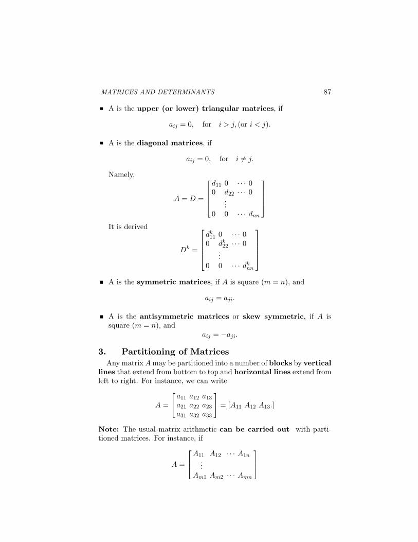
MATRICES AND DETERMINANTS 87
A is the upper (or lower) triangular matrices, if
aij = 0, for i > j, (or i < j).
A is the diagonal matrices, if
aij = 0, for i 6= j.
Namely,
A = D =
d11 0 · · · 00 d22 · · · 0
...0 0 · · · dnn
It is derived
Dk =
dk11 0 · · · 0
0 dk22 · · · 0
...0 0 · · · dk
nn
A is the symmetric matrices, if A is square (m = n), and
aij = aji.
A is the antisymmetric matrices or skew symmetric, if A issquare (m = n), and
aij = −aji.
3. Partitioning of MatricesAny matrix A may be partitioned into a number of blocks by vertical
lines that extend from bottom to top and horizontal lines extend fromleft to right. For instance, we can write
A =
a11 a12 a13
a21 a22 a23
a31 a32 a33
= [A11 A12 A13.]
Note: The usual matrix arithmetic can be carried out with parti-tioned matrices. For instance, if
A =
A11 A12 · · · A1n...
Am1 Am2 · · · Amn
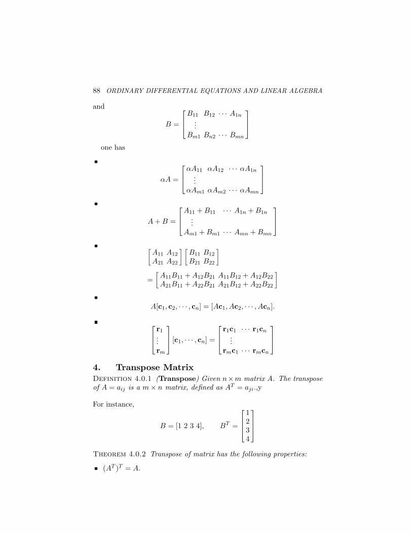
88 ORDINARY DIFFERENTIAL EQUATIONS AND LINEAR ALGEBRA
and
B =
B11 B12 · · · A1n...
Bm1 Bn2 · · · Bmn
one has
αA =
αA11 αA12 · · · αA1n...
αAm1 αAm2 · · · αAmn
A + B =
A11 + B11 · · · A1n + B1n...
Am1 + Bm1 · · · Amn + Bmn
[A11 A12
A21 A22
] [B11 B12
B21 B22
]
=[A11B11 + A12B21 A11B12 + A12B22
A21B11 + A22B21 A21B12 + A22B22
]
A[c1, c2, · · · , cn] = [Ac1, Ac2, · · · , Acn].
r1...rm
[c1, · · · , cn] =
r1c1 · · · r1cn...
rmc1 · · · rmcn
4. Transpose MatrixDefinition 4.0.1 (Transpose) Given n×m matrix A. The transposeof A = aij is a m× n matrix, defined as AT = aji.,y
For instance,
B = [1 2 3 4], BT =
1234
Theorem 4.0.2 Transpose of matrix has the following properties:
(AT )T = A.
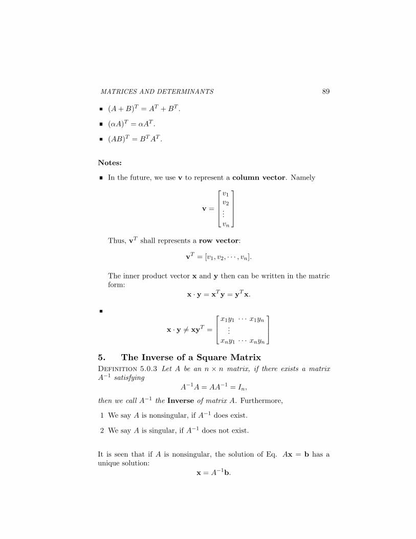
MATRICES AND DETERMINANTS 89
(A + B)T = AT + BT .
(αA)T = αAT .
(AB)T = BT AT .
Notes:
In the future, we use v to represent a column vector. Namely
v =
v1
v2...vn
Thus, vT shall represents a row vector:
vT = [v1, v2, · · · , vn].
The inner product vector x and y then can be written in the matricform:
x · y = xTy = yTx.
x · y 6= xyT =
x1y1 · · · x1yn...
xny1 · · · xnyn
5. The Inverse of a Square MatrixDefinition 5.0.3 Let A be an n × n matrix, if there exists a matrixA−1 satisfying
A−1A = AA−1 = In,
then we call A−1 the Inverse of matrix A. Furthermore,
1 We say A is nonsingular, if A−1 does exist.
2 We say A is singular, if A−1 does not exist.
It is seen that if A is nonsingular, the solution of Eq. Ax = b has aunique solution:
x = A−1b.
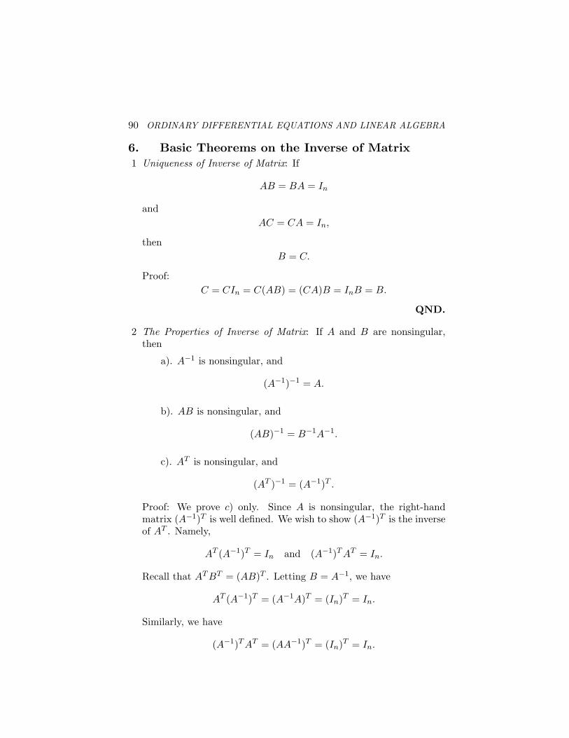
90 ORDINARY DIFFERENTIAL EQUATIONS AND LINEAR ALGEBRA
6. Basic Theorems on the Inverse of Matrix1 Uniqueness of Inverse of Matrix: If
AB = BA = In
andAC = CA = In,
thenB = C.
Proof:C = CIn = C(AB) = (CA)B = InB = B.
QND.
2 The Properties of Inverse of Matrix: If A and B are nonsingular,then
a). A−1 is nonsingular, and
(A−1)−1 = A.
b). AB is nonsingular, and
(AB)−1 = B−1A−1.
c). AT is nonsingular, and
(AT )−1 = (A−1)T .
Proof: We prove c) only. Since A is nonsingular, the right-handmatrix (A−1)T is well defined. We wish to show (A−1)T is the inverseof AT . Namely,
AT (A−1)T = In and (A−1)T AT = In.
Recall that AT BT = (AB)T . Letting B = A−1, we have
AT (A−1)T = (A−1A)T = (In)T = In.
Similarly, we have
(A−1)T AT = (AA−1)T = (In)T = In.
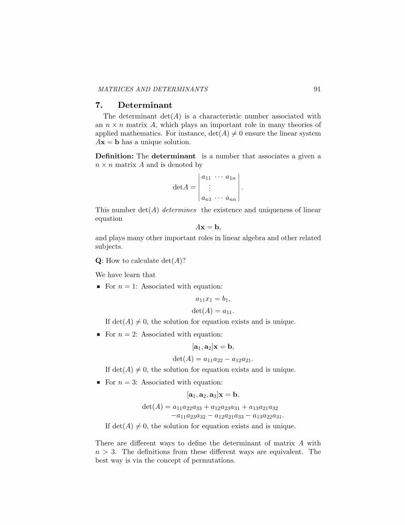
MATRICES AND DETERMINANTS 91
7. DeterminantThe determinant det(A) is a characteristic number associated with
an n × n matrix A, which plays an important role in many theories ofapplied mathematics. For instance, det(A) 6= 0 ensure the linear systemAx = b has a unique solution.
Definition: The determinant is a number that associates a given an× n matrix A and is denoted by
detA =
∣∣∣∣∣∣∣
a11 · · · a1n...
an1 · · · ann
∣∣∣∣∣∣∣.
This number det(A) determines the existence and uniqueness of linearequation
Ax = b,
and plays many other important roles in linear algebra and other relatedsubjects.
Q: How to calculate det(A)?
We have learn that
For n = 1: Associated with equation:
a11x1 = b1,
det(A) = a11.
If det(A) 6= 0, the solution for equation exists and is unique.
For n = 2: Associated with equation:
[a1,a2]x = b,
det(A) = a11a22 − a12a21.
If det(A) 6= 0, the solution for equation exists and is unique.
For n = 3: Associated with equation:
[a1,a2,a3]x = b,
det(A) = a11a22a33 + a12a23a31 + a13a21a32
−a11a23a32 − a12a21a33 − a13a22a31.
If det(A) 6= 0, the solution for equation exists and is unique.
There are different ways to define the determinant of matrix A withn > 3. The definitions from these different ways are equivalent. Thebest way is via the concept of permutations.
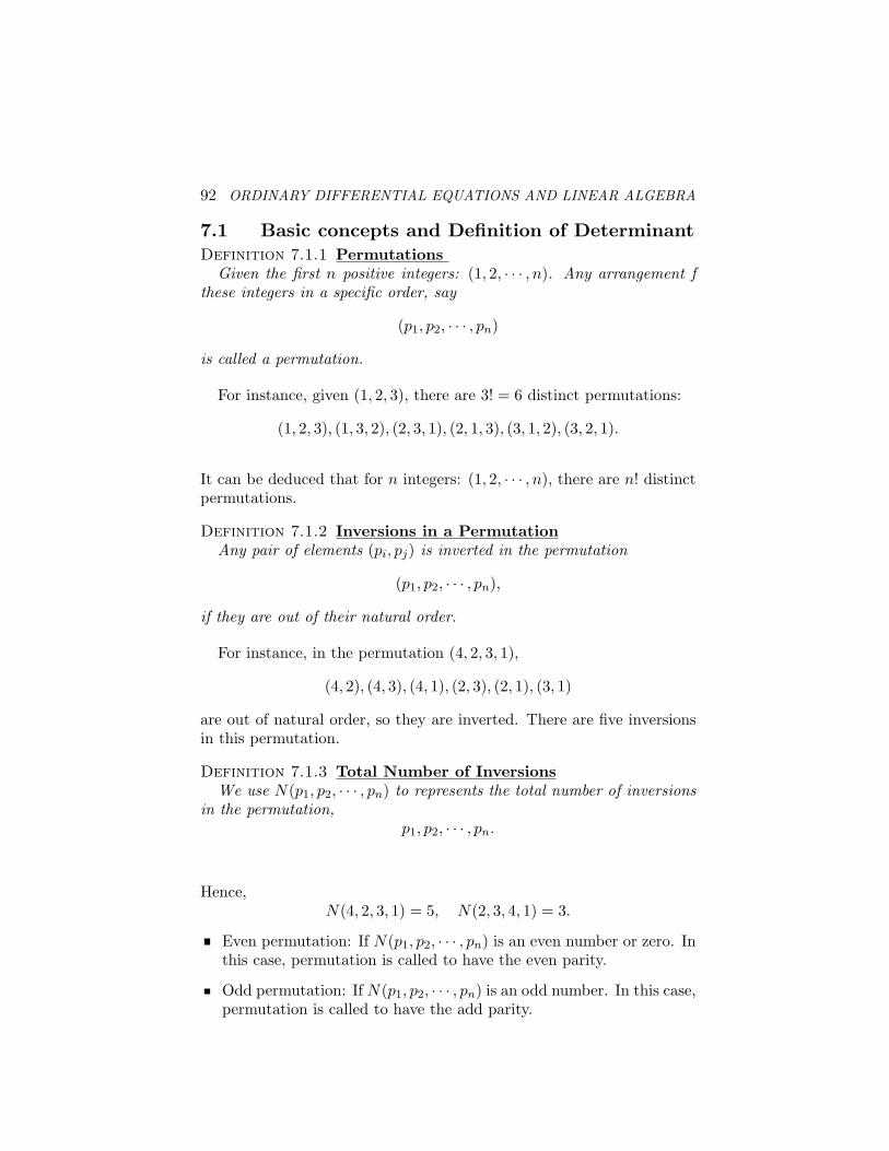
92 ORDINARY DIFFERENTIAL EQUATIONS AND LINEAR ALGEBRA
7.1 Basic concepts and Definition of DeterminantDefinition 7.1.1 Permutations
Given the first n positive integers: (1, 2, · · · , n). Any arrangement fthese integers in a specific order, say
(p1, p2, · · · , pn)
is called a permutation.
For instance, given (1, 2, 3), there are 3! = 6 distinct permutations:
(1, 2, 3), (1, 3, 2), (2, 3, 1), (2, 1, 3), (3, 1, 2), (3, 2, 1).
It can be deduced that for n integers: (1, 2, · · · , n), there are n! distinctpermutations.
Definition 7.1.2 Inversions in a PermutationAny pair of elements (pi, pj) is inverted in the permutation
(p1, p2, · · · , pn),
if they are out of their natural order.
For instance, in the permutation (4, 2, 3, 1),
(4, 2), (4, 3), (4, 1), (2, 3), (2, 1), (3, 1)
are out of natural order, so they are inverted. There are five inversionsin this permutation.
Definition 7.1.3 Total Number of InversionsWe use N(p1, p2, · · · , pn) to represents the total number of inversions
in the permutation,p1, p2, · · · , pn.
Hence,N(4, 2, 3, 1) = 5, N(2, 3, 4, 1) = 3.
Even permutation: If N(p1, p2, · · · , pn) is an even number or zero. Inthis case, permutation is called to have the even parity.
Odd permutation: If N(p1, p2, · · · , pn) is an odd number. In this case,permutation is called to have the add parity.
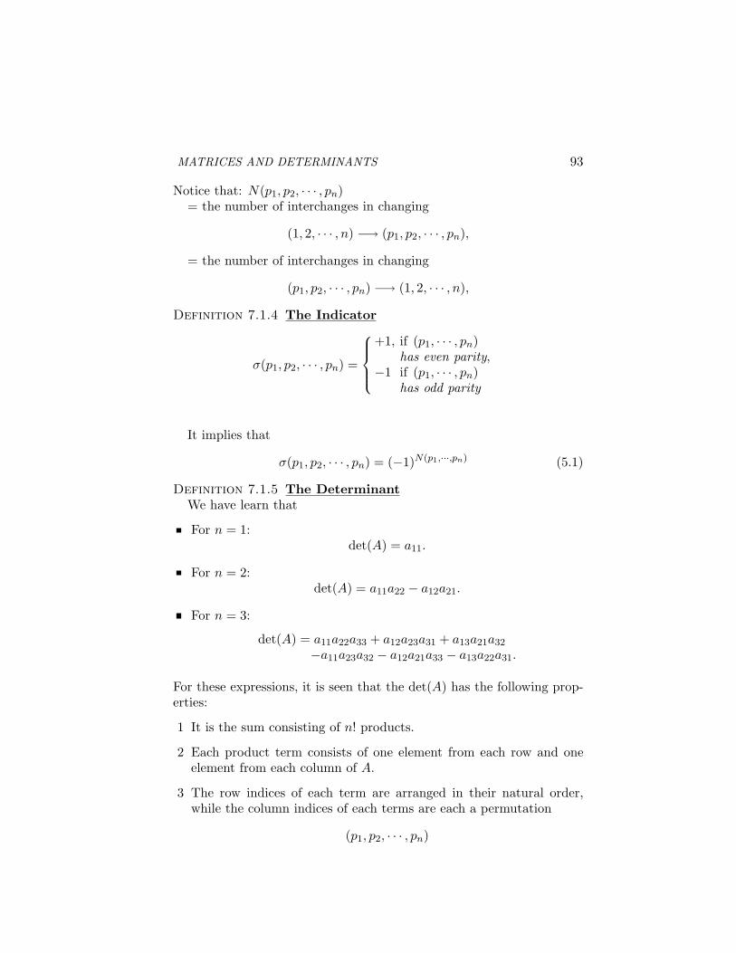
MATRICES AND DETERMINANTS 93
Notice that: N(p1, p2, · · · , pn)= the number of interchanges in changing
(1, 2, · · · , n) −→ (p1, p2, · · · , pn),
= the number of interchanges in changing
(p1, p2, · · · , pn) −→ (1, 2, · · · , n),
Definition 7.1.4 The Indicator
σ(p1, p2, · · · , pn) =
+1, if (p1, · · · , pn)has even parity,
−1 if (p1, · · · , pn)has odd parity
It implies that
σ(p1, p2, · · · , pn) = (−1)N(p1,···,pn) (5.1)
Definition 7.1.5 The DeterminantWe have learn that
For n = 1:det(A) = a11.
For n = 2:det(A) = a11a22 − a12a21.
For n = 3:
det(A) = a11a22a33 + a12a23a31 + a13a21a32
−a11a23a32 − a12a21a33 − a13a22a31.
For these expressions, it is seen that the det(A) has the following prop-erties:
1 It is the sum consisting of n! products.
2 Each product term consists of one element from each row and oneelement from each column of A.
3 The row indices of each term are arranged in their natural order,while the column indices of each terms are each a permutation
(p1, p2, · · · , pn)
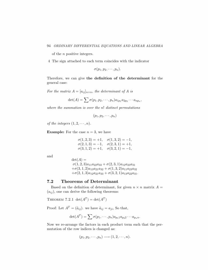
94 ORDINARY DIFFERENTIAL EQUATIONS AND LINEAR ALGEBRA
of the n positive integers.
4 The sign attached to each term coincides with the indicator
σ(p1, p2, · · · , pn).
Therefore, we can give the definition of the determinant for thegeneral case:
For the matrix A = [aij ]n×n, the determinant of A is
det(A) =∑
σ(p1, p2, · · · , pn)a1p1a2p2 · · · anpn ,
where the summation is over the n! distinct permutations
(p1, p2, · · · , pn)
of the integers (1, 2, · · · , n).
Example: For the case n = 3, we have
σ(1, 2, 3) = +1, σ(1, 3, 2) = −1,σ(2, 1, 3) = −1, σ(2, 3, 1) = +1,σ(3, 1, 2) = +1, σ(3, 2, 1) = −1,
anddet(A) =σ(1, 2, 3)a11a22a33 + σ(2, 3, 1)a12a23a31
+σ(3, 1, 2)a13a21a32 + σ(1, 3, 2)a11a23a32
+σ(2, 1, 3)a12a21a33 + σ(3, 2, 1)a13a22a31.
7.2 Theorems of DeterminantBased on the definition of determinant, for given n × n matrix A =
(aij), one can derive the following theorems:
Theorem 7.2.1 det(AT ) = det(AT )
Proof: Let AT = (aij). we have aij = aji, So that,
det(AT ) =∑
σ(p1, · · · , pn)ap11ap22 · · · apnn.
Now we re-arrange the factors in each product term such that the per-mutation of the row indices is changed as:
(p1, p2, · · · , pn) −→ (1, 2, · · · , n).
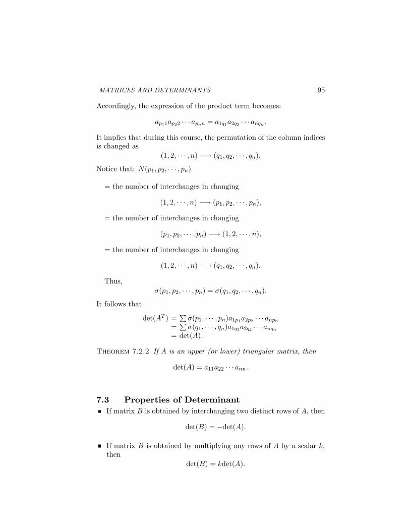
MATRICES AND DETERMINANTS 95
Accordingly, the expression of the product term becomes:
ap11ap22 · · · apnn = a1q1a2q2 · · · anqn .
It implies that during this course, the permutation of the column indicesis changed as
(1, 2, · · · , n) −→ (q1, q2, · · · , qn).
Notice that: N(p1, p2, · · · , pn)
= the number of interchanges in changing
(1, 2, · · · , n) −→ (p1, p2, · · · , pn),
= the number of interchanges in changing
(p1, p2, · · · , pn) −→ (1, 2, · · · , n),
= the number of interchanges in changing
(1, 2, · · · , n) −→ (q1, q2, · · · , qn).
Thus,σ(p1, p2, · · · , pn) = σ(q1, q2, · · · , qn).
It follows that
det(AT ) =∑
σ(p1, · · · , pn)a1p1a2p2 · · · anpn
=∑
σ(q1, · · · , qn)a1q1a2q2 · · · anqn
= det(A).
Theorem 7.2.2 If A is an upper (or lower) triangular matrix, then
det(A) = a11a22 · · · ann.
7.3 Properties of DeterminantIf matrix B is obtained by interchanging two distinct rows of A, then
det(B) = −det(A).
If matrix B is obtained by multiplying any rows of A by a scalar k,then
det(B) = kdet(A).
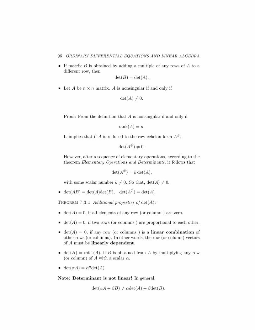
96 ORDINARY DIFFERENTIAL EQUATIONS AND LINEAR ALGEBRA
If matrix B is obtained by adding a multiple of any rows of A to adifferent row, then
det(B) = det(A).
Let A be n× n matrix. A is nonsingular if and only if
det(A) 6= 0.
Proof: From the definition that A is nonsingular if and only if
rank(A) = n.
It implies that if A is reduced to the row echelon form A#,
det(A#) 6= 0.
However, after a sequence of elementary operations, according to thetheorem Elementary Operations and Determinants, it follows that
det(A#) = k det(A),
with some scalar number k 6= 0. So that, det(A) 6= 0.
det(AB) = det(A)det(B), det(AT ) = det(A)
Theorem 7.3.1 Additional properties of det(A):
det(A) = 0, if all elements of any row (or column ) are zero.
det(A) = 0, if two rows (or columns ) are proportional to each other.
det(A) = 0, if any row (or columns ) is a linear combination ofother rows (or columns). In other words, the row (or column) vectorsof A must be linearly dependent.
det(B) = αdet(A), if B is obtained from A by multiplying any row(or column) of A with a scalar α.
det(αA) = αndet(A).
Note: Determinant is not linear! In general,
det(αA + βB) 6= αdet(A) + βdet(B).
MATRICES AND DETERMINANTS 97
7.4 Minor, Co-factors, AdjointDefinition 7.4.1 (Minor) Let A be n × n matrix. The minor, Mij,of the element aij is the determinant of the matrix obtained by deletingthe ith row vector and jth column vector of A .
Definition 7.4.2 (Co-factor) Let A be n × n matrix. The co-factor,Aij, of the element aij is defined as
Aij = (−1)i+jMij .
Definition 7.4.3 (matrix of co-factor) Let A = (aij) be n × n ma-trix. The matrix of co-factor is defined as
(Aij) =
A11, A12, · · · , A1n
A21, A22, · · · , A2n...An1, An2, · · · , Ann
.
Definition 7.4.4 (adjoint of matrix ) Let A = (aij) be n×n matrix.The adjoint of matrix A is defined as
adj(A) = (Aij)T = (Aji) =
A11, A21, · · · , An1
A12, A22, · · · , An2...A1n, A2n, · · · , Ann
.
We give the following important theorem without proving.
Theorem 7.4.5 (Co-factor Expansion Theorem) Let A be n × n
matrix. We can make the following expansions.The expansion along ith row:
det(A) = ai1Ai1 + ai2Ai2 + · · ·+ ainAin. (5.2)
The expansion along ith column:
det(A) = a1iA1i + a2iA2i + · · ·+ aniAni. (5.3)
Theorem 7.4.6 (Summation of elements of ith row (or column)multiplied by the co-factors of j-th row’s (or column’s) element)
Let A be n× n matrix. We have the following summations.
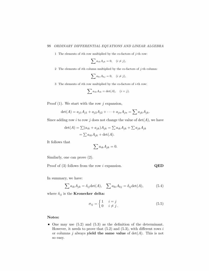
98 ORDINARY DIFFERENTIAL EQUATIONS AND LINEAR ALGEBRA
1 The elements of ith row multiplied by the co-factors of j-th row:
∑aikAjk = 0, (i 6= j),
2 The elements of ith column multiplied by the co-factors of j-th column:
∑akiAkj = 0, (i 6= j),
3 The elements of ith row multiplied by the co-factors of i-th row:
∑aikAik = det(A), (i = j).
Proof (1). We start with the row j expansion,
det(A) = aj1Aj1 + aj2Aj2 + · · ·+ ajnAjn =∑
ajkAjk.
Since adding row i to row j does not change the value of det(A), we have
det(A) =∑
(aik + ajk)Ajk =∑
aikAjk +∑
ajkAjk
=∑
aikAjk + det(A).
It follows that ∑aikAjk = 0.
Similarly, one can prove (2).
Proof of (3) follows from the row i expansion. QED
In summary, we have:∑
aikAjk = δijdet(A),∑
akiAkj = δijdet(A), (5.4)
where δij is the Kronecker delta:
σij ={
1 i = j0 i 6= j .
(5.5)
Notes:
One may use (5.2) and (5.3) as the definition of the determinant.However, it needs to prove that (5.2) and (5.3), with different rows ior columns j always yield the same value of det(A). This is notso easy.
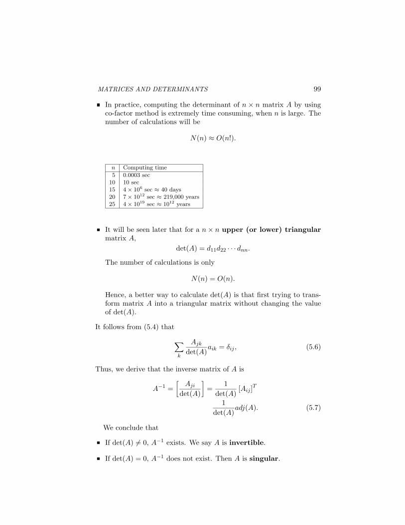
MATRICES AND DETERMINANTS 99
In practice, computing the determinant of n × n matrix A by usingco-factor method is extremely time consuming, when n is large. Thenumber of calculations will be
N(n) ≈ O(n!).
n Computing time
5 0.0003 sec10 10 sec15 4× 10⁶ sec ≈ 40 days20 7× 10¹² sec ≈ 219,000 years25 4× 10¹⁹ sec ≈ 1012 years
It will be seen later that for a n× n upper (or lower) triangularmatrix A,
det(A) = d11d22 · · · dnn.
The number of calculations is only
N(n) = O(n).
Hence, a better way to calculate det(A) is that first trying to trans-form matrix A into a triangular matrix without changing the valueof det(A).
It follows from (5.4) that
∑
k
Ajk
det(A)aik = δij , (5.6)
Thus, we derive that the inverse matrix of A is
A−1 =[
Aji
det(A)
]=
1det(A)
[Aij ]T
1det(A)
adj(A). (5.7)
We conclude that
If det(A) 6= 0, A−1 exists. We say A is invertible.
If det(A) = 0, A−1 does not exist. Then A is singular.
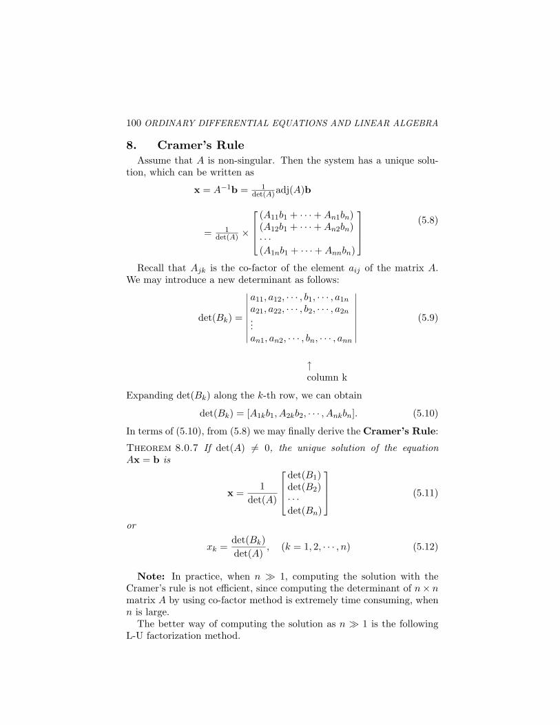
100 ORDINARY DIFFERENTIAL EQUATIONS AND LINEAR ALGEBRA
8. Cramer’s RuleAssume that A is non-singular. Then the system has a unique solu-
tion, which can be written as
x = A−1b = 1det(A)adj(A)b
= 1det(A) ×
(A11b1 + · · ·+ An1bn)(A12b1 + · · ·+ An2bn)· · ·(A1nb1 + · · ·+ Annbn)
(5.8)
Recall that Ajk is the co-factor of the element aij of the matrix A.We may introduce a new determinant as follows:
det(Bk) =
∣∣∣∣∣∣∣∣∣
a11, a12, · · · , b1, · · · , a1n
a21, a22, · · · , b2, · · · , a2n...an1, an2, · · · , bn, · · · , ann
∣∣∣∣∣∣∣∣∣(5.9)
↑column k
Expanding det(Bk) along the k-th row, we can obtain
det(Bk) = [A1kb1, A2kb2, · · · , Ankbn]. (5.10)
In terms of (5.10), from (5.8) we may finally derive the Cramer’s Rule:
Theorem 8.0.7 If det(A) 6= 0, the unique solution of the equationAx = b is
x =1
det(A)
det(B1)det(B2)· · ·det(Bn)
(5.11)
or
xk =det(Bk)det(A)
, (k = 1, 2, · · · , n) (5.12)
Note: In practice, when n À 1, computing the solution with theCramer’s rule is not efficient, since computing the determinant of n× nmatrix A by using co-factor method is extremely time consuming, whenn is large.
The better way of computing the solution as n À 1 is the followingL-U factorization method.
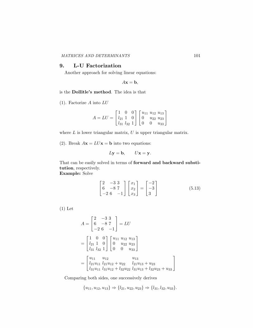
MATRICES AND DETERMINANTS 101
9. L-U FactorizationAnother approach for solving linear equations:
Ax = b,
is the Dollitle’s method. The idea is that
(1). Factorize A into LU
A = LU =
1 0 0l21 1 0l31 l32 1
u11 u12 u13
0 u22 u23
0 0 u33
where L is lower triangular matrix, U is upper triangular matrix.
(2). Break Ax = LUx = b into two equations:
Ly = b, Ux = y.
That can be easily solved in terms of forward and backward substi-tution, respectively.Example: Solve
2 −3 36 −8 7−2 6 −1
x1
x2
x3
=
−2−33
(5.13)
(1) Let
A =
2 −3 36 −8 7−2 6 −1
= LU
=
1 0 0l21 1 0l31 l32 1
u11 u12 u13
0 u22 u23
0 0 u33
=
u11 u12 u13
l21u11 l21u12 + u22 l21u13 + u23
l31u11 l31u12 + l32u22 l31u13 + l32u23 + u33
Comparing both sides, one successively derives
{u11, u12, u13} ⇒ {l21, u22, u23} ⇒ {l31, l32, u33}.
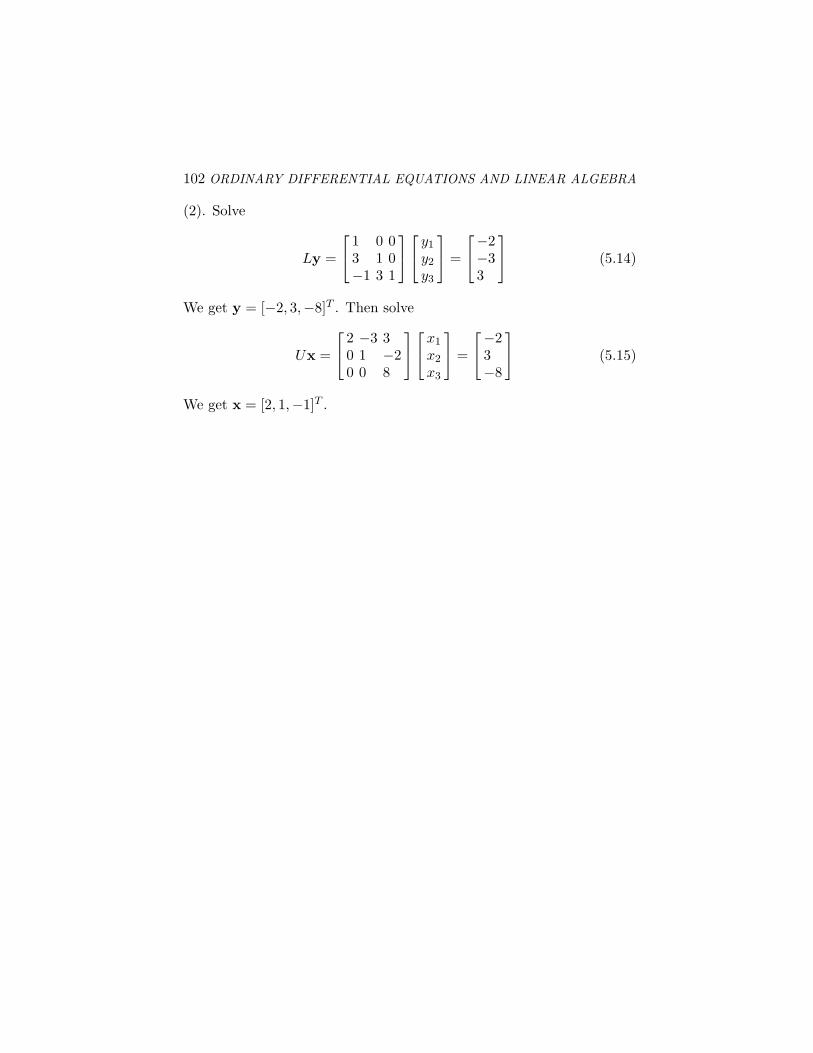
102 ORDINARY DIFFERENTIAL EQUATIONS AND LINEAR ALGEBRA
(2). Solve
Ly =
1 0 03 1 0−1 3 1
y1
y2
y3
=
−2−33
(5.14)
We get y = [−2, 3,−8]T . Then solve
Ux =
2 −3 30 1 −20 0 8
x1
x2
x3
=
−23−8
(5.15)
We get x = [2, 1,−1]T .
Chapter 6
VECTOR SPACE—DEFINITIONS AND BASICCONCEPTS
1. Introduction and Motivation1.1 A brief Review of Geometric Vectors in 3D
spaceWe meet vectors for the first time in studying calculus and mechan-
ics. There, a vector v in 3D physical space, represents some physicalquantity, such as velocity, force, ... .
A vector v can be described geometrically by an arrow, which isdetermined by its magnitude and direction.
However, if one introduces a coordinate system {e1, e2, e3} in the 3Dspace, the geometric vector v can be described by its coordinatesas
v = (v1, v2, v3) = v1e1 + v2e2 + v3e3.
under this coordinate system.
The most important properties of a set of vectors in 3D space are thatone can introduce the following operations on it:
Addition: w = v + v;
Scalar Multiplication: w=cv.
Now, let us consider linear problems,
L(x) = 0,
where L is any type of linear operators:
103
104 ORDINARY DIFFERENTIAL EQUATIONS AND LINEAR ALGEBRA
The two typical cases are
Linear homogeneous algebraic equation:
Ax = 0, L = A =
1 − 1 22 − 2 43 − 3 6
.
It has a general solution:
x1 = (x2 − 2x3), x2 = r, x3 = s
with any numbers r, s. We may write
x = c1(1, 1, 0) + c2(−2, 0, 1),
orx = c1x1 + c2x2,
where c1, c2 are arbitrary constants, while
x1 = (1, 1, 0), x2 = (−2, 0, 1),
are a pair of fundamental solutions.
Linear homogeneous ODE:
y′′ + y = 0, L = (D2 + 1).
It has a general solution:
y = c1y1(x) + c2y2(x),
where c1, c2 are arbitrary constants, while
y1 = cosx, y2 = sinx,
are a pair of fundamental solutions.
These two problems with different operators have very similar mathe-matical structure:
1 The operators both act on some types of mathematical objects, like
x, triples of ordered numbers;y(x), all differentiable functions defined on some interval (I).
These objects may be generally called as vectors.
2 The general solutions of both systems can be expressed by linearcombination of a set of fundamental solutions.
Thus, one can attempt to discuss all linear problems in the sameframe-work, as some abstract concepts are introduced.
VECTOR SPACE—DEFINITIONS AND BASIC CONCEPTS 105
2. Definition of a Vector SpaceWe start with considering the set of all geometric vectors denoted by
V .
It is known that one can define two operations on all elements of V :
The addition.
Multiply a vector by a real number
The important thing is that these two operations are subject to thefollowing properties:
1 V is closed under these operations, namely
For any pair u;v ∈ V ,
u + v = w ∈ V.
for any vector u ∈ V , and any real number r:
ru = w ∈ V.
2 The vector addition is communicative and associative:
u + v = v + u,
u + (v + w) = (u + v) + w,
3 There exists a vector called the zero vector, 0 ∈ V , such that
u + 0 = u.
4 For any u ∈ V , there exits a vector −u, called the additive inversevector of u, such that
u + (−u) = 0.
5 For any pair u;v ∈ V , and any real numbers r, s:
r(u + v) = ru + rv, (r + s)u = ru + su,
rsu = r(su), 1u = u.
Now, one may extend the above geometrical vectors to the generalvector space.
106 ORDINARY DIFFERENTIAL EQUATIONS AND LINEAR ALGEBRA
Definition 2.0.1 (Vector Space ) A nonempty set V whose elementsare called vectors is said to form a vector space (over F), provided thefollowing conditions are satisfied:
1 The two operations: the addition and scalar multiplication with anyscalars in F can be defined over V ;
2 These two operation are subjects the rules the same as given to geo-metric vectors described as above.
Remark 2.0.2 The key point is that the vector space has four compo-nents ( V, F , +, · ):
1 A nonempty set of vectors, V .
2 A set of scalars F (either R, or C ).
3 The operation (+) defined on V .
4 The operation of scalar multiplication (·) defined on V .
3. Examples of Vector Spaces1 V = Rn is the set of all ordered n-tuples:
x = (x1, x2, · · · , xn), xi ∈ R (i =, 2, · · · , n)
with the zero vector,(0, 0, · · · , 0);
and the operations:
x + y = (x1, x2, · · · , xn) + (y1, y2, · · · , yn)(x1 + y1, x2 + y2, · · · , xn + yn)
andrx = r(x1, x2, · · · , xn) = (rx1, rx2, · · · , rxn).
This (V,R,+ ·) is a vector space and called the vector space Rn.
2 V = C0[a, b] is a set of all real valued continuous functions {f(x)}defined on the interval (I) = [a, b] with the operations:
(f + g)(x) = f(x) + g(x); (rf)(x) = rf(x);
the zero vector,f(x) ≡ 0.
This real function space (V,R, + ·) is a vector space.
3 V = M2 is the set of all real matrices A of 2× 2 with real elements,and the zero vector, (
0 00 0
)= 02
This (V,R,+ ·) is a vector space.
VECTOR SPACE—DEFINITIONS AND BASIC CONCEPTS 107
4. SubspacesDefinition 4.0.3 Let S is a nonempty subset of vector space V . If Sitself is a vector space under the same operations of addition and scalarmultiplication as in V , then we say that S is a subspace of V .
Theorem 4.0.4 S is a subspace of V , if and only if S is closed underthe operations of addition and scalar multiplication
5. Linear Combinations andSpanning Sets
Definition 5.0.5 A vector v in vector space V is said to be lineat com-bination of vectors v1,v2, · · · ,vk in V , if there exists scalars c1, c2, · · · , ck,such that
v = c1v1 + c2v2 + · · · ,+ckvk.
Definition 5.0.6 Let v1,v2, · · · ,vn be vectors in a vector space V . Ifevery vector in V can be written in a linear combination of v1,v2, · · · ,vn,then
we say V is spanned by v1,v2, · · · ,vn; and write
V = span{v1,v2, · · · ,vn}.
and call the set of v1,v2, · · · ,vn a spanning set in V .
For examples:
1 R3 is spanned by vectors:
v1 = (1, 0, 0),v2 = (0, 1, 0),v3 = (0, 0, 1),
because any vector v = (a, b, c) ∈ R3 can be written in the linearcombination:
v = av1 + bv2 + v3.
Hence, we haveR3 = span{v1,v2,v3}.
2 R2 is spanned by vectors:
v1 = (1, 1),v2 = (−1, 1),
108 ORDINARY DIFFERENTIAL EQUATIONS AND LINEAR ALGEBRA
because for any vector v = (a, b) ∈ R2, one can find a pair of con-stants c1, c2, such that
v = (a, b) = c1v1 + c2v2
= (c1 − c2, c1 + c2).
3 Let S be the set of all solutions of ODE:
y′′ + y = 0, x ∈ (I).
ThenS = span{ cos(x), sin(x)}
6. Linear Dependence and IndependenceDefinition 6.0.7 A set of vector {v1,v1, · · · ,vn} in a vector space Vis linear dependence, if there exists scalars
c1, c2, · · · , cn,
not all zero, such that
c1v1 + c2v2 + · · ·+ cnvn = 0.
Definition 6.0.8 A set of vector {v1,v1, · · · ,vn} in a vector space Vis linear independence, if the only values of scalars c1, c2, · · · , cn, forwhich
c1v1 + c2v2 + · · ·+ cnvn = 0,
arec1 = c2 = · · · = cn = 0.
7. Bases and DimensionsDefinition 7.0.9 A set of vectors {v1,v1, · · · ,vn} in a vector space Vis called a basis for V , if
These vectors are linearly independent;
These vectors span V . Namely,
V = span{v1,v1, · · · ,vn}.
Definition 7.0.10 If the number of vectors in the base of vector spaceV is finite, then
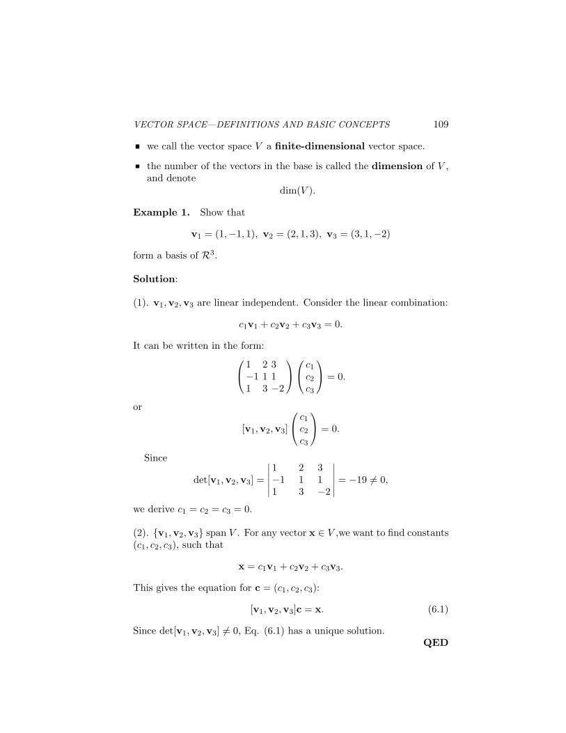
VECTOR SPACE—DEFINITIONS AND BASIC CONCEPTS 109
we call the vector space V a finite-dimensional vector space.
the number of the vectors in the base is called the dimension of V ,and denote
dim(V ).
Example 1. Show that
v1 = (1,−1, 1), v2 = (2, 1, 3), v3 = (3, 1,−2)
form a basis of R3.
Solution:
(1). v1,v2,v3 are linear independent. Consider the linear combination:
c1v1 + c2v2 + c3v3 = 0.
It can be written in the form:
1 2 3−1 1 11 3 −2
c1
c2
c3
= 0.
or
[v1,v2,v3]
c1
c2
c3
= 0.
Since
det[v1,v2,v3] =
∣∣∣∣∣∣
1 2 3−1 1 11 3 −2
∣∣∣∣∣∣= −19 6= 0,
we derive c1 = c2 = c3 = 0.
(2). {v1,v2,v3} span V . For any vector x ∈ V ,we want to find constants(c1, c2, c3), such that
x = c1v1 + c2v2 + c3v3.
This gives the equation for c = (c1, c2, c3):
[v1,v2,v3]c = x. (6.1)
Since det[v1,v2,v3] 6= 0, Eq. (6.1) has a unique solution.QED
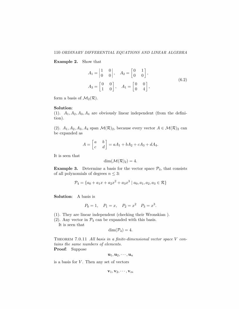
110 ORDINARY DIFFERENTIAL EQUATIONS AND LINEAR ALGEBRA
Example 2. Show that
A1 =∣∣∣∣1 00 0
∣∣∣∣ , A2 =[0 10 0
],
A3 =[0 01 0
], A1 =
[0 00 4
],
(6.2)
form a basis of M2(R).
Solution:(1). A1, A2, A3, A4 are obviously linear independent (from the defini-tion).
(2). A1, A2, A3, A4 span M(R)2, because every vector A ∈ M(R)2 canbe expanded as
A =[a bc d
]= aA1 + bA2 + cA3 + dA4.
It is seen thatdim(M(R)2) = 4.
Example 3. Determine a basis for the vector space P4, that consistsof all polynomials of degrees n ≤ 3:
P4 = {a0 + a1x + a2x2 + a3x
3 | a0, a1, a2, a3 ∈ R}
Solution: A basis is
P0 = 1, P1 = x, P2 = x2 P3 = x3.
(1). They are linear independent (checking their Wronskian ).(2). Any vector in P4 can be expanded with this basis.
It is seen thatdim(P4) = 4.
Theorem 7.0.11 All basis in a finite-dimensional vector space V con-tains the same numbers of elements.Proof: Suppose
u1,u2, · · · ,un
is a basis for V . Then any set of vectors
v1,v2, · · · ,vm
VECTOR SPACE—DEFINITIONS AND BASIC CONCEPTS 111
with (m > n), must be linear dependent. Based on the fact that everyvector of vk, (k = 1, · · ·m) can be expanded with the basis
u1,u2, · · · ,un,
it is easy to show that one can find c1, · · · , cm not all zero, such that
c1v1 + c2v2 + · · ·+ cmvm = 0.
Theorem 7.0.12 If a finite-dimensional vector has a basis consisting ofn numbers of elements, then any set of more than n vectors is linearlydependentProof: The proof is similar to the previous one. In fact, suppose
u1,u2, · · · ,un
is a basis for V and we have a set of vectors
v1,v2, · · · ,vm
with (m > n). To prove {v1,v2, · · · ,vm} is linearly dependent, oneneeds to show that there exists constants c1, · · · , cm not all zero, suchthat
c1v1 + c2v2 + · · ·+ cmvm = 0. (6.3)
However, we can make the expansions:
vj =m∑
i=1
aijui, (j = 1, 2, · · · ,m). (6.4)
By substituting (6.4) into (6.3), it results in a system of algebraic equa-tions of (m× n), which has non zero solutions, c1, · · · , cm.
Theorem 7.0.13 If a finite-dimensional vector has a basis consistingof n numbers of elements, then any spanning set for V must contains atleast n vectors.Proof: Suppose
u1,u2, · · · ,un
is a basis for V , and
V = span{v1,v2, · · · ,vm}.We need to prove m ≥ n. In fact, if m < n, then {v1, · · · ,vm} must belinear dependent, otherwise, it would be a basis of V . That is not true,as m < n.
112 ORDINARY DIFFERENTIAL EQUATIONS AND LINEAR ALGEBRA
However, from linear dependent vectors {v1, · · · ,vm}, we can alwaysfind a subset of linear independent vectors:
{v1, · · · ,vk}, (k < m).
Thus,V = span{v1,v2, · · · ,vk}, (k < m < n).
It implies that{v1,v2, · · · ,vk}, (k < m < n).
is a basis for V , and dim(V ) = k < n. It leads to the contradiction.
Theorem 7.0.14 If dim(V ) = n, the any set of n linear independentvectors in V must form a basis for V .Proof: Suppose
u1,u2, · · · ,un
are linear independent. We need to prove that any vector u ∈ V can beexpanded with this set of vectors. This is true, because the set of (n+1)vectors,
{u,u1,u2, · · · ,un}must be linear dependent.
Chapter 7
INNER PRODUCT SPACES AND THE GRAM-SCHMIDT ORTHOGONALIZATIONPROCEDURE
1. IntroductionIn this section, we are going to extend the the idea of dot product
for geometric vectors to a general vector space. With the dot product,one can define length and orthogonality in the vector space.
Recall that for two geometric vectors in R3 space,
x = (x1, x2, x3) y = (y1, y2, y3),
one has the inner product
x · y = ‖x‖ ‖y‖ cos θ
= (x1y1 + x2y2 + x3y3).
Based on this inner product, one can introduce the length of thevector,
‖x‖2 = x · x = x21 + x2
2 + x23.
and further the angle between two vectors:
cos θ =x · y
‖x‖ ‖y‖ .
Thus, one may define two vectors x, y orthogonal, if and only if
x · y = 0.
Now for a general vector space, by defining the inner product, we canalso introduce the geometric concepts of length or norm, orthogonality.
We start with the vector space Rn.
113
114 ORDINARY DIFFERENTIAL EQUATIONS AND LINEAR ALGEBRA
1.1 Definition of Inner Product in Rn
Definition 1.1.1 Given two vectors in Rn,
x = (x1, x2, · · · , xn), y = (y1, y2, · · · , yn).
We define the standard inner product, < x,y >, in Rn by
< x,y >= x · y = x1y1 + x2y2 + · · ·+ xnyn. (7.1)
The norm of x is
‖x‖ =√
< x,x > =√
x21 + x2
2 + · · ·+ x2n. (7.2)
Due to ‖x‖ ≥ 0 for any x ∈ V , we can prove that
1.1.1 Schwarz Inequality
| < x,y > | = |x · y| ≤ ‖x‖ ‖y‖ .
or|x · y|‖x‖ ‖y‖ ≤ 1.
Thus, it is possible to define the angle θ between two vectors:
cos θ =x · y
‖x‖ ‖y‖ .
Proof: As for any number α,
‖x + αy‖ = (x + αy) · (x + αy) ≥ 0,
we haveF (α) = ‖x‖2 + 2α < x,y > +α2 ‖y‖2
= aα2 + 2bα + c ≥ 0,
F (α) is a quadratic function of α, which cannot have two real roots.Therefore, we deduce that b2 − ac ≤ 0, namely
< x,y >2 −‖x‖2 ‖y‖2 ≤ 0.
INNER PRODUCT SPACES 115
1.1.2 Triangle Inequality
‖x + y‖ ≤ ‖x‖+ ‖y‖ .
Proof:‖x + y‖2 = (x + y) · (x + y)
= x · x + 2x · y + y · y≤ ‖x‖2 + 2 ‖x‖ ‖y‖+ ‖y‖2 ≤ (‖x‖+ ‖y‖)2
1.2 Basic Properties of the Inner Product in Rn
It is seen that for all vectors, x,y, z in Rn, and all real number c, wehave
1 < x,x >≥ 0, and < x,x >= 0, if and only if x = 0.
2 < x,y >=< y,x > .
3 < cx,y >= c < x,y > .
4 < x + y, z >=< x, z > + < y, z > .
2. Definition of a Real Inner ProductSpace
Definition 2.0.1 (inner product) Let V be a real vector space. Aninner product in V is a mapping that associates a real number withany pair of vectors x,y ∈ V , denoted by
< x,y >= x · y,
and satisfies the following properties:For all vectors, x,y, z in V , and all real number c,
1 < x,x >≥ 0, and < x,x >= 0, if and only if x = 0.
2 < x,y >=< y,x > .
3 < cx,y >= c < x,y > .
4 < x + y, z >=< x, z > + < y, z > .
Definition 2.0.2 (inner product space) A vector space is called in-ner product space, provided an inner product is defined in it.
Definition 2.0.3 (Norm) Let V be an inner product vector space, anorm is number that associates with every vector x in V , denoted by‖x‖ and satisfies the following properties:
116 ORDINARY DIFFERENTIAL EQUATIONS AND LINEAR ALGEBRA
1 ‖x‖ ≥ 0, and ‖x‖ = 0, if and only if x = 0.
2 ‖cx‖ = |c| ‖x‖ .
3 Triangle inequality: ‖x + y‖ ≤ ‖x‖+ ‖y‖ .
Notes:
The standard norm is defined through the inner product. Namely,‖x‖2 = x · x.
With the standard norm, the Schwarz inequality and triangle inequal-ity automatically hold.
Example: Let C0[a, b] denote the vector space of all continuous func-tions on interval [a, b]. We can define the inner product:
< f, g >=∫ b
af(x)g(x)dx.
One can prove that
< f, f >=∫ b
af2(x)dx ≥ 0;
and
< f, f >=∫ b
af2(x)dx = 0,
if and only if f(x) = 0 on [a, b]. Other inner properties are easy to proveas well.
3. Definition of a Complex Inner ProductSpace
Definition 3.0.4 Let V be a complex vector space. An inner prod-uct in V is a mapping that associates a complex number with any pairof vectors u,v ∈ V , denoted by < u,v >, and satisfies the followingproperties.
For all vectors, u,v,w in V , and all scalars (real or complex number)c,
1 < u,u >≥ 0, and < u,u >= 0, if and only if u = 0.(Note: < u,u > must be a real number!)
2 < u,v >= < v,u >.
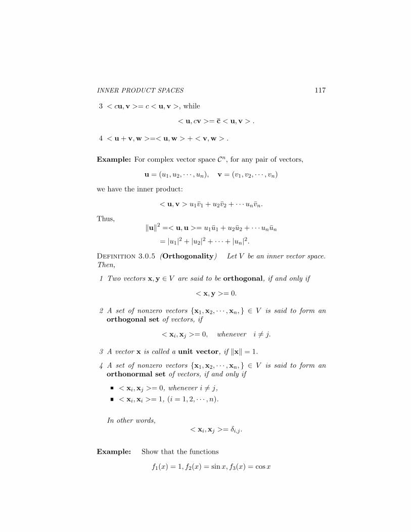
INNER PRODUCT SPACES 117
3 < cu,v >= c < u,v >, while
< u, cv >= c < u,v > .
4 < u + v,w >=< u,w > + < v,w > .
Example: For complex vector space Cn, for any pair of vectors,
u = (u1, u2, · · · , un), v = (v1, v2, · · · , vn)
we have the inner product:
< u,v > u1v1 + u2v2 + · · ·unvn.
Thus,‖u‖2 =< u,u >= u1u1 + u2u2 + · · ·unun
= |u1|2 + |u2|2 + · · ·+ |un|2.Definition 3.0.5 (Orthogonality) Let V be an inner vector space.Then,
1 Two vectors x,y ∈ V are said to be orthogonal, if and only if
< x,y >= 0.
2 A set of nonzero vectors {x1,x2, · · · ,xn, } ∈ V is said to form anorthogonal set of vectors, if
< xi,xj >= 0, whenever i 6= j.
3 A vector x is called a unit vector, if ‖x‖ = 1.
4 A set of nonzero vectors {x1,x2, · · · ,xn, } ∈ V is said to form anorthonormal set of vectors, if and only if
< xi,xj >= 0, whenever i 6= j,< xi,xi >= 1, (i = 1, 2, · · · , n).
In other words,< xi,xj >= δi,j .
Example: Show that the functions
f1(x) = 1, f2(x) = sinx, f3(x) = cosx
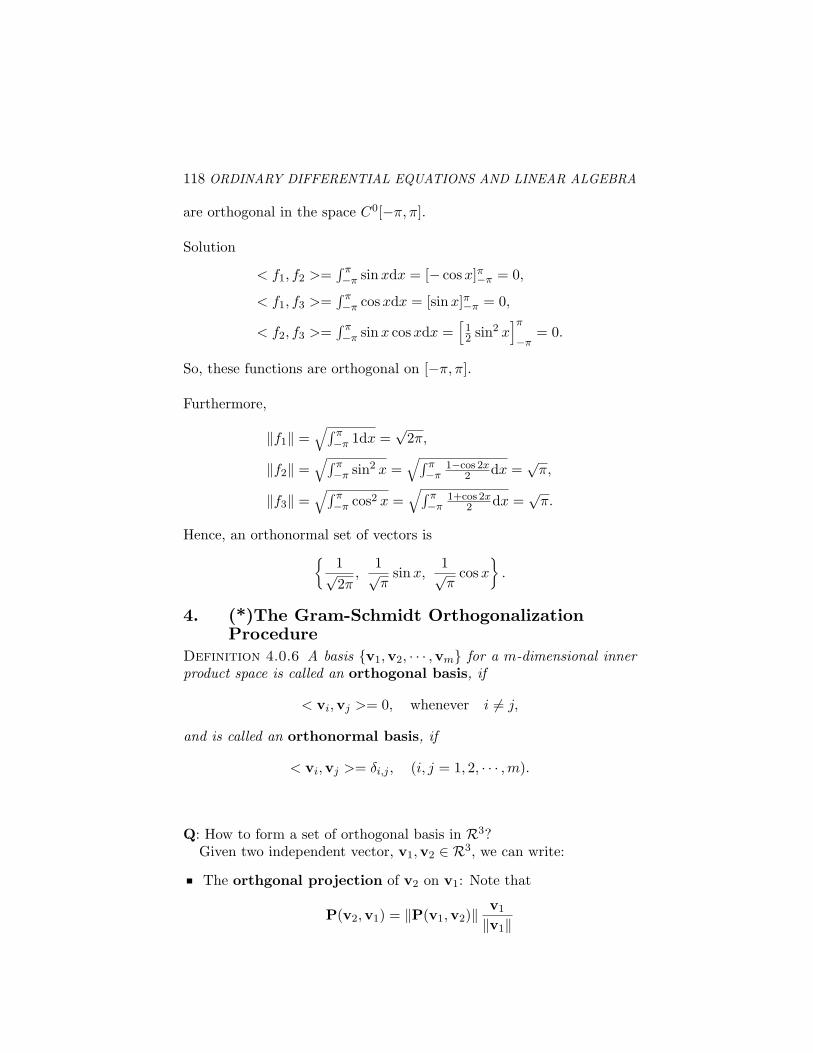
118 ORDINARY DIFFERENTIAL EQUATIONS AND LINEAR ALGEBRA
are orthogonal in the space C0[−π, π].
Solution
< f1, f2 >=∫ π−π sinxdx = [− cosx]π−π = 0,
< f1, f3 >=∫ π−π cosxdx = [sinx]π−π = 0,
< f2, f3 >=∫ π−π sinx cosxdx =
[12 sin2 x
]π
−π= 0.
So, these functions are orthogonal on [−π, π].
Furthermore,
‖f1‖ =√∫ π
−π 1dx =√
2π,
‖f2‖ =√∫ π
−π sin2 x =√∫ π
−π1−cos 2x
2 dx =√
π,
‖f3‖ =√∫ π
−π cos2 x =√∫ π
−π1+cos 2x
2 dx =√
π.
Hence, an orthonormal set of vectors is{
1√2π
,1√π
sinx,1√π
cosx
}.
4. (*)The Gram-Schmidt OrthogonalizationProcedure
Definition 4.0.6 A basis {v1,v2, · · · ,vm} for a m-dimensional innerproduct space is called an orthogonal basis, if
< vi,vj >= 0, whenever i 6= j,
and is called an orthonormal basis, if
< vi,vj >= δi,j , (i, j = 1, 2, · · · , m).
Q: How to form a set of orthogonal basis in R3?Given two independent vector, v1,v2 ∈ R3, we can write:
The orthgonal projection of v2 on v1: Note that
P(v2,v1) = ‖P(v1,v2)‖ v1
‖v1‖
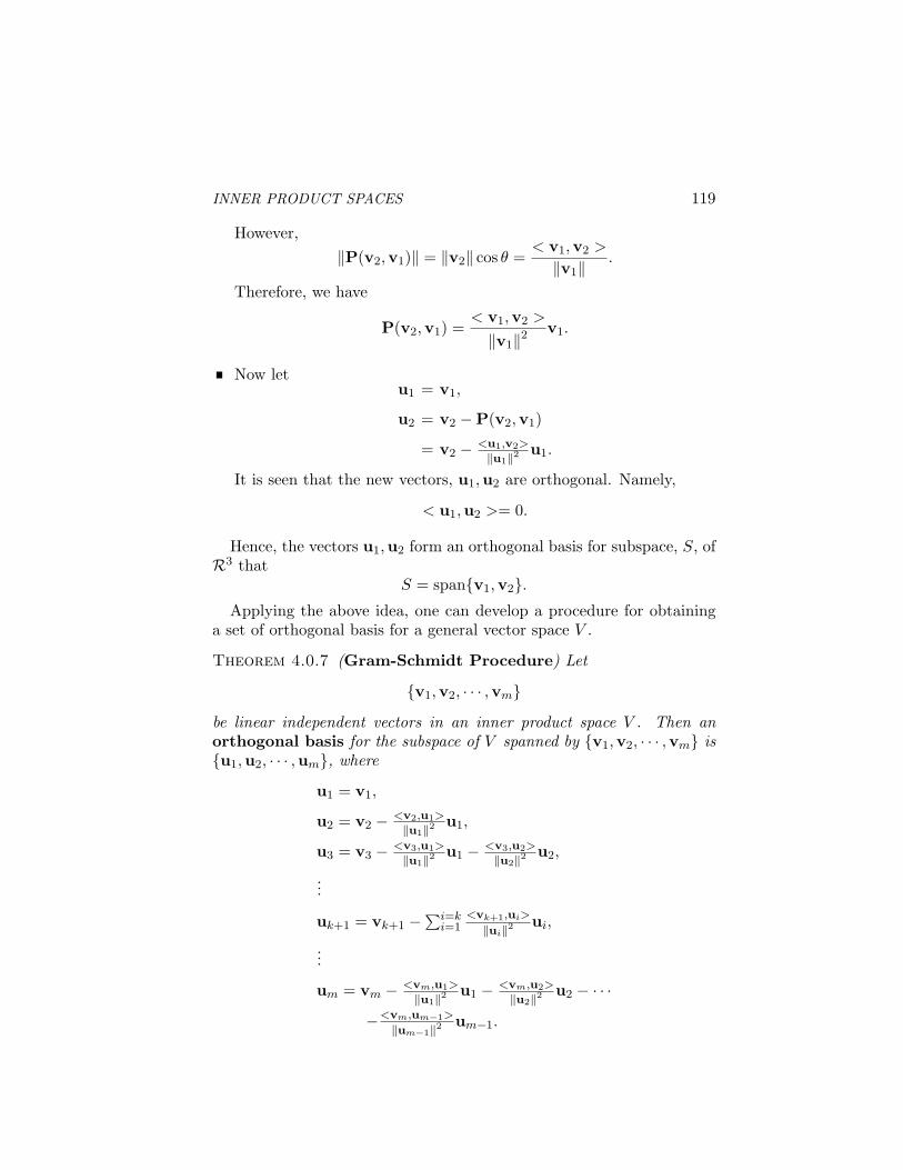
INNER PRODUCT SPACES 119
However,‖P(v2,v1)‖ = ‖v2‖ cos θ =
< v1,v2 >
‖v1‖ .
Therefore, we have
P(v2,v1) =< v1,v2 >
‖v1‖2 v1.
Now letu1 = v1,
u2 = v2 −P(v2,v1)
= v2 − <u1,v2>
‖u1‖2 u1.
It is seen that the new vectors, u1,u2 are orthogonal. Namely,
< u1,u2 >= 0.
Hence, the vectors u1,u2 form an orthogonal basis for subspace, S, ofR3 that
S = span{v1,v2}.Applying the above idea, one can develop a procedure for obtaining
a set of orthogonal basis for a general vector space V .
Theorem 4.0.7 (Gram-Schmidt Procedure) Let
{v1,v2, · · · ,vm}be linear independent vectors in an inner product space V . Then anorthogonal basis for the subspace of V spanned by {v1,v2, · · · ,vm} is{u1,u2, · · · ,um}, where
u1 = v1,
u2 = v2 − <v2,u1>
‖u1‖2 u1,
u3 = v3 − <v3,u1>
‖u1‖2 u1 − <v3,u2>
‖u2‖2 u2,
...
uk+1 = vk+1 −∑i=k
i=1<vk+1,ui>
‖ui‖2 ui,
...
um = vm − <vm,u1>
‖u1‖2 u1 − <vm,u2>
‖u2‖2 u2 − · · ·−<vm,um−1>
‖um−1‖2 um−1.
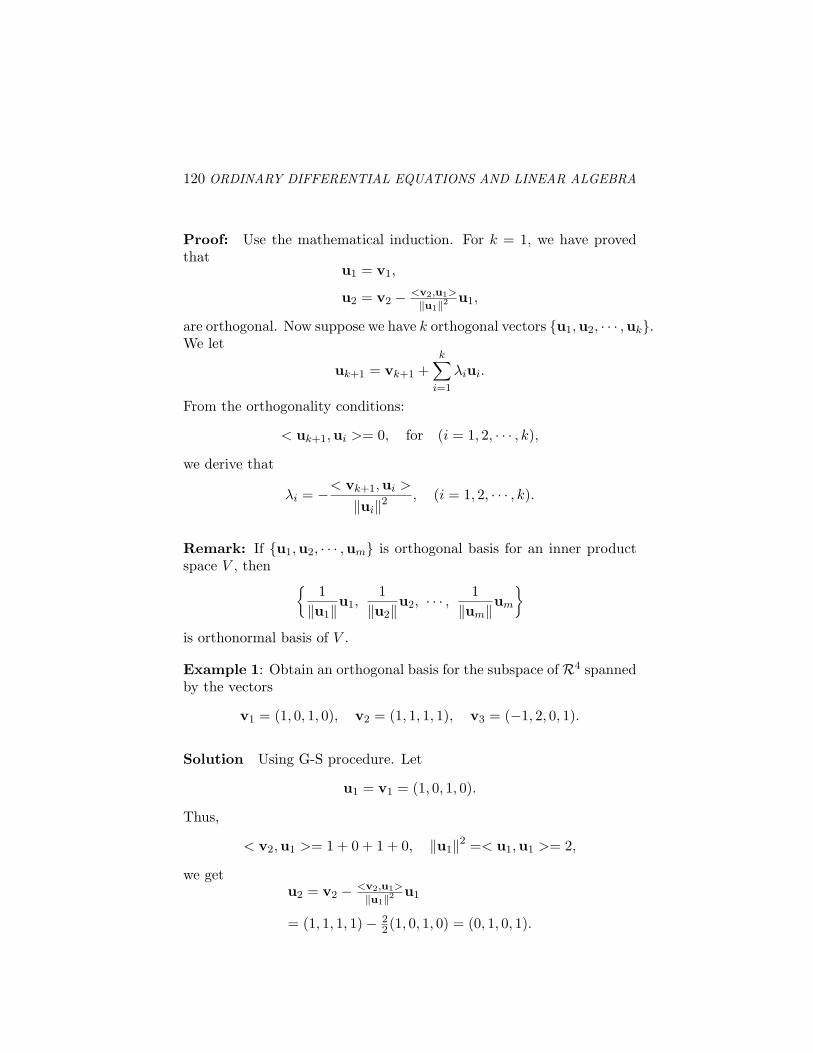
120 ORDINARY DIFFERENTIAL EQUATIONS AND LINEAR ALGEBRA
Proof: Use the mathematical induction. For k = 1, we have provedthat
u1 = v1,
u2 = v2 − <v2,u1>
‖u1‖2 u1,
are orthogonal. Now suppose we have k orthogonal vectors {u1,u2, · · · ,uk}.We let
uk+1 = vk+1 +k∑
i=1
λiui.
From the orthogonality conditions:
< uk+1,ui >= 0, for (i = 1, 2, · · · , k),
we derive that
λi = −< vk+1,ui >
‖ui‖2 , (i = 1, 2, · · · , k).
Remark: If {u1,u2, · · · ,um} is orthogonal basis for an inner productspace V , then
{1
‖u1‖u1,1
‖u2‖u2, · · · , 1‖um‖um
}
is orthonormal basis of V .
Example 1: Obtain an orthogonal basis for the subspace ofR4 spannedby the vectors
v1 = (1, 0, 1, 0), v2 = (1, 1, 1, 1), v3 = (−1, 2, 0, 1).
Solution Using G-S procedure. Let
u1 = v1 = (1, 0, 1, 0).
Thus,
< v2,u1 >= 1 + 0 + 1 + 0, ‖u1‖2 =< u1,u1 >= 2,
we getu2 = v2 − <v2,u1>
‖u1‖2 u1
= (1, 1, 1, 1)− 22(1, 0, 1, 0) = (0, 1, 0, 1).
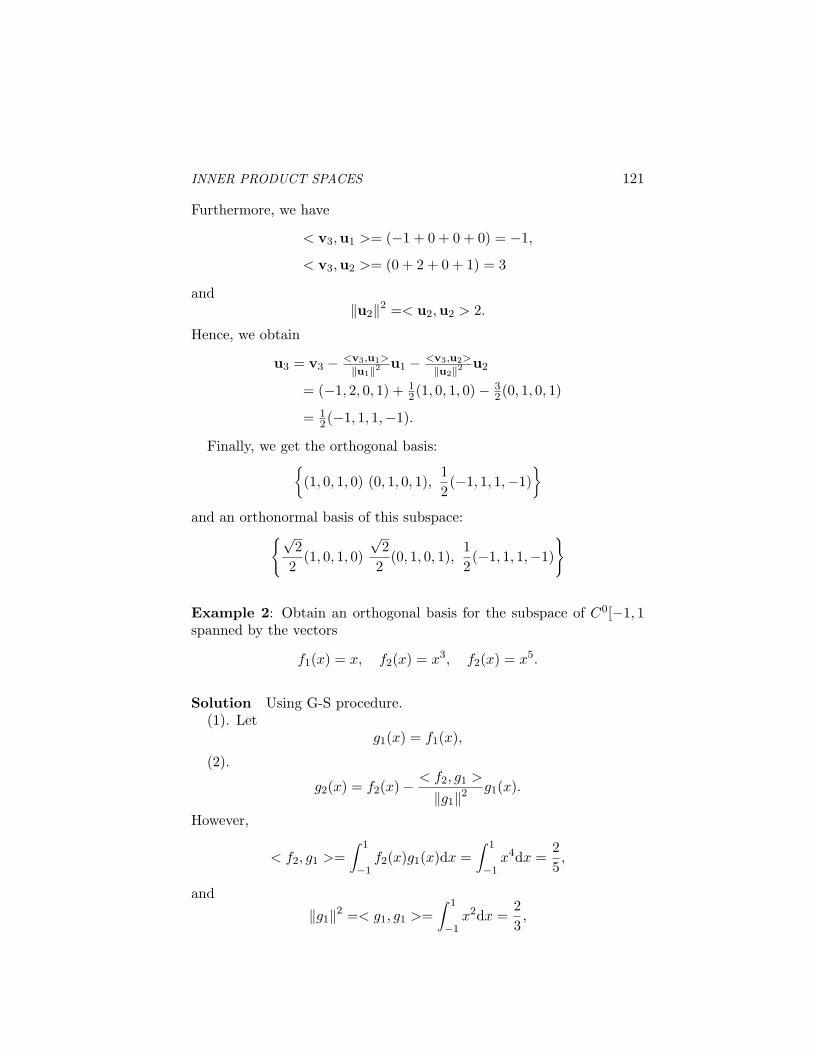
INNER PRODUCT SPACES 121
Furthermore, we have
< v3,u1 >= (−1 + 0 + 0 + 0) = −1,
< v3,u2 >= (0 + 2 + 0 + 1) = 3
and‖u2‖2 =< u2,u2 > 2.
Hence, we obtain
u3 = v3 − <v3,u1>
‖u1‖2 u1 − <v3,u2>
‖u2‖2 u2
= (−1, 2, 0, 1) + 12(1, 0, 1, 0)− 3
2(0, 1, 0, 1)
= 12(−1, 1, 1,−1).
Finally, we get the orthogonal basis:{
(1, 0, 1, 0) (0, 1, 0, 1),12(−1, 1, 1,−1)
}
and an orthonormal basis of this subspace:{√
22
(1, 0, 1, 0)√
22
(0, 1, 0, 1),12(−1, 1, 1,−1)
}
Example 2: Obtain an orthogonal basis for the subspace of C0[−1, 1spanned by the vectors
f1(x) = x, f2(x) = x3, f2(x) = x5.
Solution Using G-S procedure.(1). Let
g1(x) = f1(x),
(2).
g2(x) = f2(x)− < f2, g1 >
‖g1‖2 g1(x).
However,
< f2, g1 >=∫ 1
−1f2(x)g1(x)dx =
∫ 1
−1x4dx =
25,
and
‖g1‖2 =< g1, g1 >=∫ 1
−1x2dx =
23,
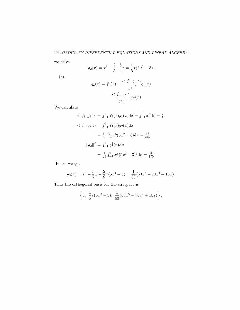
122 ORDINARY DIFFERENTIAL EQUATIONS AND LINEAR ALGEBRA
we driveg2(x) = x3 − 2
5· 32x =
15x(5x2 − 3).
(3).
g3(x) = f3(x)− < f3, g1 >
‖g1‖2 g1(x)
−< f3, g2 >
‖g2‖2 g2(x).
We calculate
< f3, g1 > =∫ 1−1 f3(x)g1(x)dx =
∫ 1−1 x6dx = 2
7 ,
< f3, g2 > =∫ 1−1 f3(x)g2(x)dx
= 15
∫ 1−1 x6(5x2 − 3)dx = 16
315 ,
‖g2‖2 =∫ 1−1 g2
2(x)dx
= 125
∫ 1−1 x2(5x2 − 3)2dx = 8
175
Hence, we get
g3(x) = x3 − 37x− 2
9x(5x2 − 3) =
163
(63x5 − 70x3 + 15x).
Thus,the orthogonal basis for the subspace is{
x,15x(5x2 − 3),
163
(63x5 − 70x3 + 15x)}
.
Chapter 8
LINEAR TRANSFORMATIONS
1. IntroductionWe now are going to study the operations defined in a vector space,
or say, the mappings between two vector spaces This concept is a gen-eralization of the idea of a function of real variable.
2. DefinitionsDefinition 2.0.8 (Mapping) Let V and W be two vector spaces. Amapping, T , from V into W is a rule that associates with each vector,
x ∈ (V ) =⇒ y ∈ (W );
and write asT (x) = y.
Moreover, in this case,
vector space (V ), is called the domain of mapping T .
the set of vectors y ∈ (W ) that we can map onto is called range ofthe mapping T .
Definition 2.0.9 (Linear Transformations) Let V and W be vec-tor spaces. A mapping, T : V −→ W , from V into W is called lineartransformation (or linear operator) from V to W , if it has the followingproperties:
T (x + y) = T (x) + T (y).
T (cx) = cT (x), for all x ∈ V and all scalars c ∈ R, or c ∈ C.
123
124 ORDINARY DIFFERENTIAL EQUATIONS AND LINEAR ALGEBRA
Therefore, for a linear transformation we have
T (c1v1 + c2v2 + · · ·+ cmvm)
= c1T (v1) + c2T (v2) + · · ·+ cmT (vm).
Examples: Linear Transformations:
T : C1(I) → C0(I), byT (f) = f ′.
T : R2 → R2, by
T (x1, x2) = (x1 − x2, x1 + x2).
T : Rn →Rm, byT (x) = Ax,
where A is an m× n matrix.
Definition 2.0.10 If T1 : V → W and T2 : V → W are two lineartransformations. We say T1 = T2, if and only if
T1(v) = T2(v)
for all v ∈ V .
Definition 2.0.11 Let T1 : V → W and T2 : V → W be lineartransformations, and C be a scalar. We define the sum and scalarproduct as follows:
(T1 + T2)(v) = T1(v) + T2(v), for all v ∈ V .
(cT1)(v) = cT1(v), for all v ∈ V .
Theorem 2.0.12 Let V and W be real vector spaces. Consider theset of all linear transformation T : V → W together with the operationsof the addition and scalar multiplications defined above. Then this setforms a vector space, L(V,W ).
Proof: Leave to readers as an excise. Note that the zero vector 0 ∈L(V, W ) is the transformation: O : V → W , namely,
O(v) = 0, for all v ∈ V.
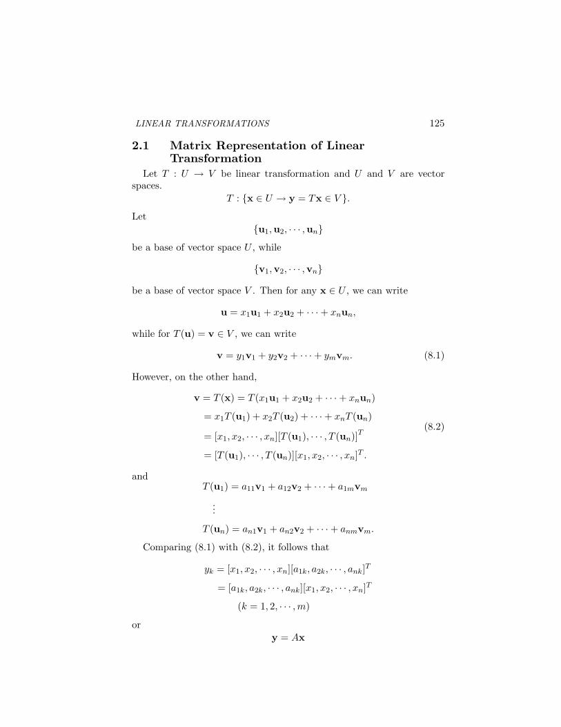
LINEAR TRANSFORMATIONS 125
2.1 Matrix Representation of LinearTransformation
Let T : U → V be linear transformation and U and V are vectorspaces.
T : {x ∈ U → y = Tx ∈ V }.Let
{u1,u2, · · · ,un}be a base of vector space U , while
{v1,v2, · · · ,vn}
be a base of vector space V . Then for any x ∈ U , we can write
u = x1u1 + x2u2 + · · ·+ xnun,
while for T (u) = v ∈ V , we can write
v = y1v1 + y2v2 + · · ·+ ymvm. (8.1)
However, on the other hand,
v = T (x) = T (x1u1 + x2u2 + · · ·+ xnun)
= x1T (u1) + x2T (u2) + · · ·+ xnT (un)
= [x1, x2, · · · , xn][T (u1), · · · , T (un)]T
= [T (u1), · · · , T (un)][x1, x2, · · · , xn]T .
(8.2)
andT (u1) = a11v1 + a12v2 + · · ·+ a1mvm
...
T (un) = an1v1 + an2v2 + · · ·+ anmvm.
Comparing (8.1) with (8.2), it follows that
yk = [x1, x2, · · · , xn][a1k, a2k, · · · , ank]T
= [a1k, a2k, · · · , ank][x1, x2, · · · , xn]T
(k = 1, 2, · · · ,m)
ory = Ax
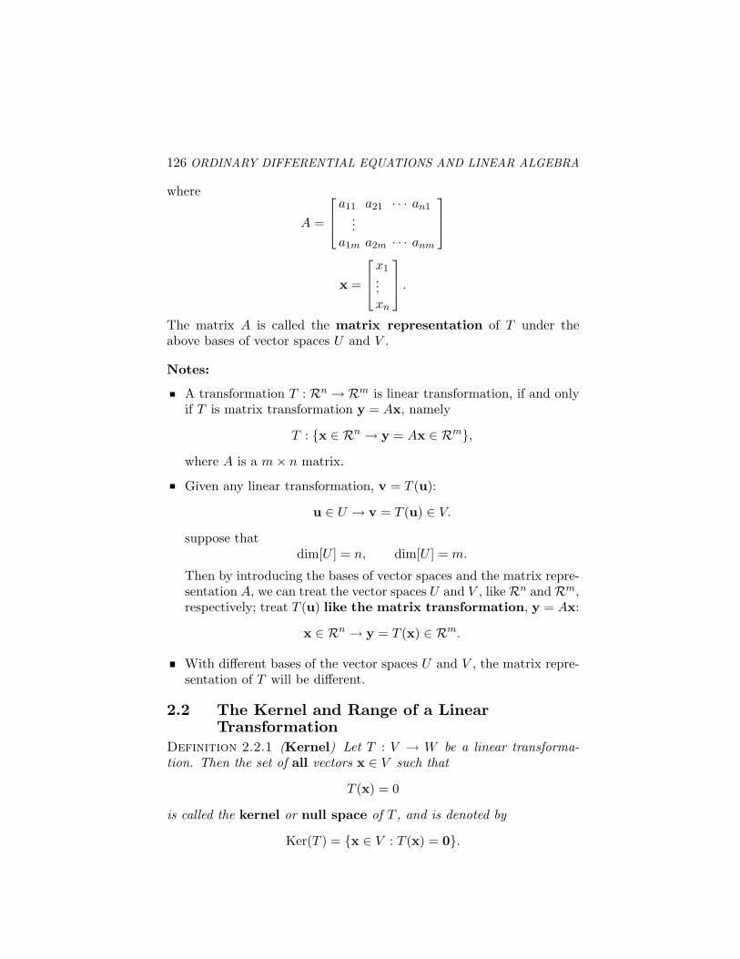
126 ORDINARY DIFFERENTIAL EQUATIONS AND LINEAR ALGEBRA
where
A =
a11 a21 · · · an1...
a1m a2m · · · anm
x =
x1...xn
.
The matrix A is called the matrix representation of T under theabove bases of vector spaces U and V .
Notes:
A transformation T : Rn → Rm is linear transformation, if and onlyif T is matrix transformation y = Ax, namely
T : {x ∈ Rn → y = Ax ∈ Rm},where A is a m× n matrix.
Given any linear transformation, v = T (u):
u ∈ U → v = T (u) ∈ V.
suppose thatdim[U ] = n, dim[U ] = m.
Then by introducing the bases of vector spaces and the matrix repre-sentation A, we can treat the vector spaces U and V , likeRn andRm,respectively; treat T (u) like the matrix transformation, y = Ax:
x ∈ Rn → y = T (x) ∈ Rm.
With different bases of the vector spaces U and V , the matrix repre-sentation of T will be different.
2.2 The Kernel and Range of a LinearTransformation
Definition 2.2.1 (Kernel) Let T : V → W be a linear transforma-tion. Then the set of all vectors x ∈ V such that
T (x) = 0
is called the kernel or null space of T , and is denoted by
Ker(T ) = {x ∈ V : T (x) = 0}.
LINEAR TRANSFORMATIONS 127
Note that T (0) = T (0v) = 0T (v) = 0. Hence,
0 ∈ Ker(T ).
Definition 2.2.2 (Range) Let T : V → W be a linear transformation.Then the set of all vectors y ∈ W such that
T (x) = y,
for at least one x ∈ V , is called the range of T , and is denoted by
Rng(T ) = {y ∈ W : T (x) = y for at least one x ∈ V }.Examples: Let T : Rn →Rm is defined by
T (x) = Ax,
where A is a m× n matrix. Then,
Ker(T ) = {x ∈ Rn : Ax = 0}.It is the set of all solutions for the homogeneous linear equation:
Ax = 0.
Furthermore,
Rng(T ) = {y ∈ Rm : Ax = y for some x ∈ Rn}.This is set vectors in Rm for which the non-homogenous system
Ax = y
is consistent.There are several important theorems regarding to the kernel and
range of T .
Theorem 2.2.3 Let T : V → W be a linear transformation. Then
Ker(T ) is a subspace of V .
Rng(T ) is a subspace of W .
Proof: It is easy. Just start from the definition of subspace.
Theorem 2.2.4 Let T : V → W be a linear transformation and V isa finite-dimensional vector space. Then
dim[Ker(T )] + dim[Rng(T )] = dim[V ].
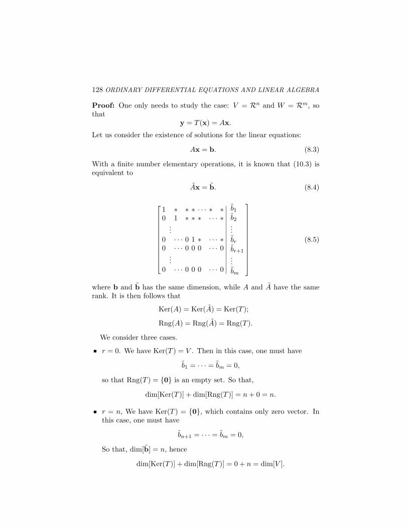
128 ORDINARY DIFFERENTIAL EQUATIONS AND LINEAR ALGEBRA
Proof: One only needs to study the case: V = Rn and W = Rm, sothat
y = T (x) = Ax.
Let us consider the existence of solutions for the linear equations:
Ax = b. (8.3)
With a finite number elementary operations, it is known that (10.3) isequivalent to
Ax = b. (8.4)
1 ∗ ∗ ∗ · · · ∗ ∗0 1 ∗ ∗ ∗ · · · ∗
...0 · · · 0 1 ∗ · · · ∗0 · · · 0 0 0 · · · 0
...0 · · · 0 0 0 · · · 0
∣∣∣∣∣∣∣∣∣∣∣∣∣∣∣∣∣
b1
b2...br
br+1...bm
(8.5)
where b and b has the same dimension, while A and A have the samerank. It is then follows that
Ker(A) = Ker(A) = Ker(T );
Rng(A) = Rng(A) = Rng(T ).
We consider three cases.
r = 0. We have Ker(T ) = V . Then in this case, one must have
b1 = · · · = bm = 0,
so that Rng(T ) = {0} is an empty set. So that,
dim[Ker(T )] + dim[Rng(T )] = n + 0 = n.
r = n, We have Ker(T ) = {0}, which contains only zero vector. Inthis case, one must have
bn+1 = · · · = bm = 0,
So that, dim[b] = n, hence
dim[Ker(T )] + dim[Rng(T )] = 0 + n = dim[V ].
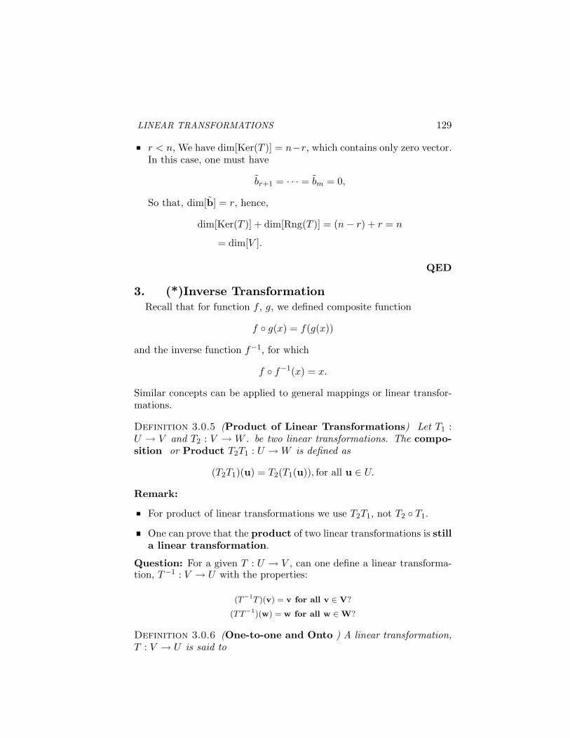
LINEAR TRANSFORMATIONS 129
r < n, We have dim[Ker(T )] = n−r, which contains only zero vector.In this case, one must have
br+1 = · · · = bm = 0,
So that, dim[b] = r, hence,
dim[Ker(T )] + dim[Rng(T )] = (n− r) + r = n
= dim[V ].
QED
3. (*)Inverse TransformationRecall that for function f , g, we defined composite function
f ◦ g(x) = f(g(x))
and the inverse function f−1, for which
f ◦ f−1(x) = x.
Similar concepts can be applied to general mappings or linear transfor-mations.
Definition 3.0.5 (Product of Linear Transformations) Let T1 :U → V and T2 : V → W . be two linear transformations. The compo-sition or Product T2T1 : U → W is defined as
(T2T1)(u) = T2(T1(u)), for all u ∈ U.
Remark:
For product of linear transformations we use T2T1, not T2 ◦ T1.
One can prove that the product of two linear transformations is stilla linear transformation.
Question: For a given T : U → V , can one define a linear transforma-tion, T−1 : V → U with the properties:
(T−1T )(v) = v for all v ∈ V?
(TT−1)(w) = w for all w ∈ W?
Definition 3.0.6 (One-to-one and Onto ) A linear transformation,T : V → U is said to
130 ORDINARY DIFFERENTIAL EQUATIONS AND LINEAR ALGEBRA
One-to-one: If x 6= y, then T (x) 6= T (y), for all x,y ∈ V .
Onto: Rng(T ) = U . Namely, every vector y ∈ U must be an imageof some vector x ∈ V .
Theorem 3.0.7 Let T : V → U be a linear transformation. Then T isone-to-one if and only if
Ker(T ) = 0.
Proof: If Ker(T ) = 0, for any x 6= y, T (x− y) 6= (0).
Definition 3.0.8 (Inverse Transformation) Let T : V → U be alinear transformation. If T is both one-to-one and onto then thelinear transformation T−1 : U → V is defined by
T−1(u) = v, if and only if T (v) = u.
Theorem 3.0.9 Consider T : Rn →Rm defined by
T (x) = Ax.
Then T−1 exists if and only if A is a non-singular n×n matrix. In sucha case,
T−1y = A−1y.
Proof: (1). A must be n× n matrix:
If n > m, Ker(T ) = 0, the transformation T cannot be not one-to-one.
If m > n, Rng(T ) 6= Rm = U , as one can prove that
dim[Ker(T )] = 0, and dim[Rng(T )] = n < m.
Furthermore,(2). A must be non-singular. Because if and only if
der(A) 6= 0,
the system of linear inhomogeneous equations
Ax = y
has a unique solution for any y ∈ U = Rn.
Example 1: Define the linear transformation, T : P2 → P2 by
T (ax + b) = (a + b)x + (a− b).
LINEAR TRANSFORMATIONS 131
Show that T−1 exists and find it.
Solution: (1). T is one-to-one.
Ker(T ) = {ax + b : (a + b)x + (a− b) = 0 ∈ P2}.It leads to
a + b = 0 a− b = 0,
so that a = b = 0. This shows Ker(T ) contains only zero polynomial,i.e.
Ker(T ) = {0}.Therefore, T is one-to-one.
(2). T is onto. From the theorem,
dim[Ker(T )] + dim[Rng(T )] = 0 + dim[Rng(T )]
= dim[V ] = dim[P2],
ordim[Rng(T )] = dim[P2] = 2
On the other hand, Rng(T ) ∈ U = P2. It is a subspace of P2. It followsthat Rng(T ) = P2. So, we deduce that T is onto
(3) From T−1((a + b)x + (a− b)) = ax + b, we derive that for any vectory,
y = Ax + b ∈ U,=⇒ x = ax + b ∈ V,
whereA = a + b, B = a− b.
It is solved that
a =12(A−B), b =
12(A + B).
Finally, we obtain
T−1(Ax + B) =12(A−B)x +
12(A + B).
Example 2: Give an IVP of ODE:
L[y] = y′′ + y = 0,y(1) = a, y′(1) = b.
(8.6)
132 ORDINARY DIFFERENTIAL EQUATIONS AND LINEAR ALGEBRA
Its solutions y(x) (1 ≤ x ≤ π) forms a vector space: V = spansinx, cosx.Define the linear transformation, T : V → R2. Show that T−1 existsand find it.
Solution: Let y1(x) = cosx, y2(x) = sinx be the basis of V ; while letx1 = [0, 1];x2 = [1, 0] be the basis of R2. Then any solution y(x) of theequation can be expressed in the form:
y(x) = c1y1 + c2y2 = c1 cosx + c2 sinx,
andy(1) = c1 cos 1 + c2 sin 1, y′(1) = −c1 sin 1 + c2 cos 1.
On the other hand, any vector x ∈ R2 is expressed as
x = ax1 + bx2.
The linear transformation can be described as
T : c = [c1, c2]T → x = [a, b]T
where[a, b]T = [c1 cos 1 + c2 sin 1,−c1 sin 1 + c2 cos 1]T
its matrix representation is:
x = [a, b]T = A[c1, c2]T
where
A =[cos 1 sin 1− sin 1 cos 1
].
The inverse of T exists, since det(A) 6= 0, and
A−1 =[cos 1 − sin 1sin 1 cos 1
].
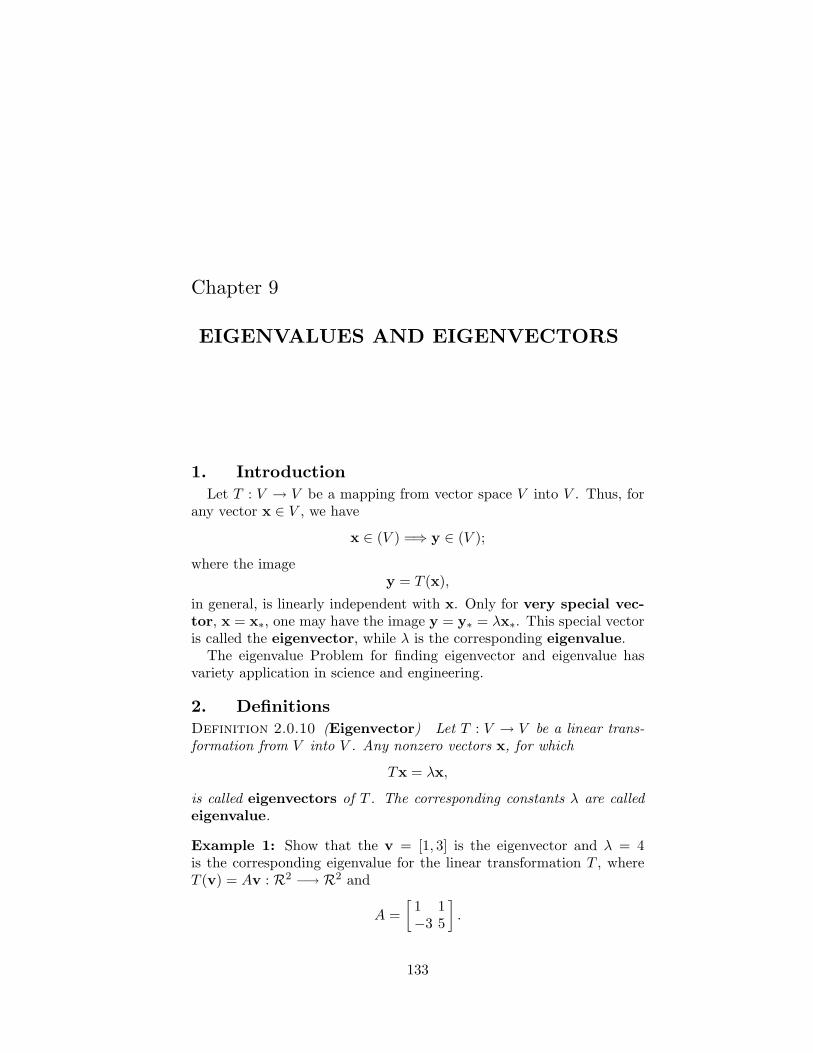
Chapter 9
EIGENVALUES AND EIGENVECTORS
1. IntroductionLet T : V → V be a mapping from vector space V into V . Thus, for
any vector x ∈ V , we have
x ∈ (V ) =⇒ y ∈ (V );
where the imagey = T (x),
in general, is linearly independent with x. Only for very special vec-tor, x = x∗, one may have the image y = y∗ = λx∗. This special vectoris called the eigenvector, while λ is the corresponding eigenvalue.
The eigenvalue Problem for finding eigenvector and eigenvalue hasvariety application in science and engineering.
2. DefinitionsDefinition 2.0.10 (Eigenvector) Let T : V → V be a linear trans-formation from V into V . Any nonzero vectors x, for which
Tx = λx,
is called eigenvectors of T . The corresponding constants λ are calledeigenvalue.
Example 1: Show that the v = [1, 3] is the eigenvector and λ = 4is the corresponding eigenvalue for the linear transformation T , whereT (v) = Av : R2 −→ R2 and
A =[1 1−3 5
].
133
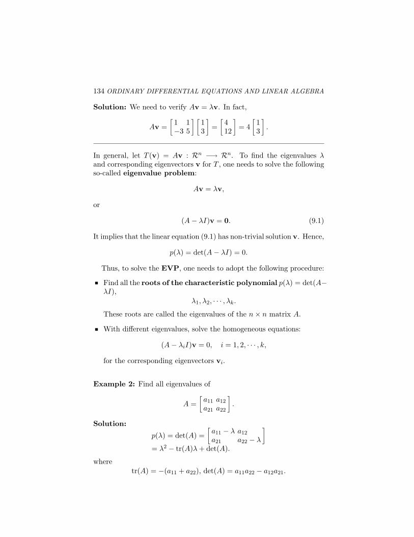
134 ORDINARY DIFFERENTIAL EQUATIONS AND LINEAR ALGEBRA
Solution: We need to verify Av = λv. In fact,
Av =[1 1−3 5
] [13
]=
[412
]= 4
[13
].
In general, let T (v) = Av : Rn −→ Rn. To find the eigenvalues λand corresponding eigenvectors v for T , one needs to solve the followingso-called eigenvalue problem:
Av = λv,
or
(A− λI)v = 0. (9.1)
It implies that the linear equation (9.1) has non-trivial solution v. Hence,
p(λ) = det(A− λI) = 0.
Thus, to solve the EVP, one needs to adopt the following procedure:
Find all the roots of the characteristic polynomial p(λ) = det(A−λI),
λ1, λ2, · · · , λk.
These roots are called the eigenvalues of the n× n matrix A.
With different eigenvalues, solve the homogeneous equations:
(A− λiI)v = 0, i = 1, 2, · · · , k,
for the corresponding eigenvectors vi.
Example 2: Find all eigenvalues of
A =[a11 a12
a21 a22
].
Solution:
p(λ) = det(A) =[a11 − λ a12
a21 a22 − λ
]
= λ2 − tr(A)λ + det(A).
wheretr(A) = −(a11 + a22), det(A) = a11a22 − a12a21.
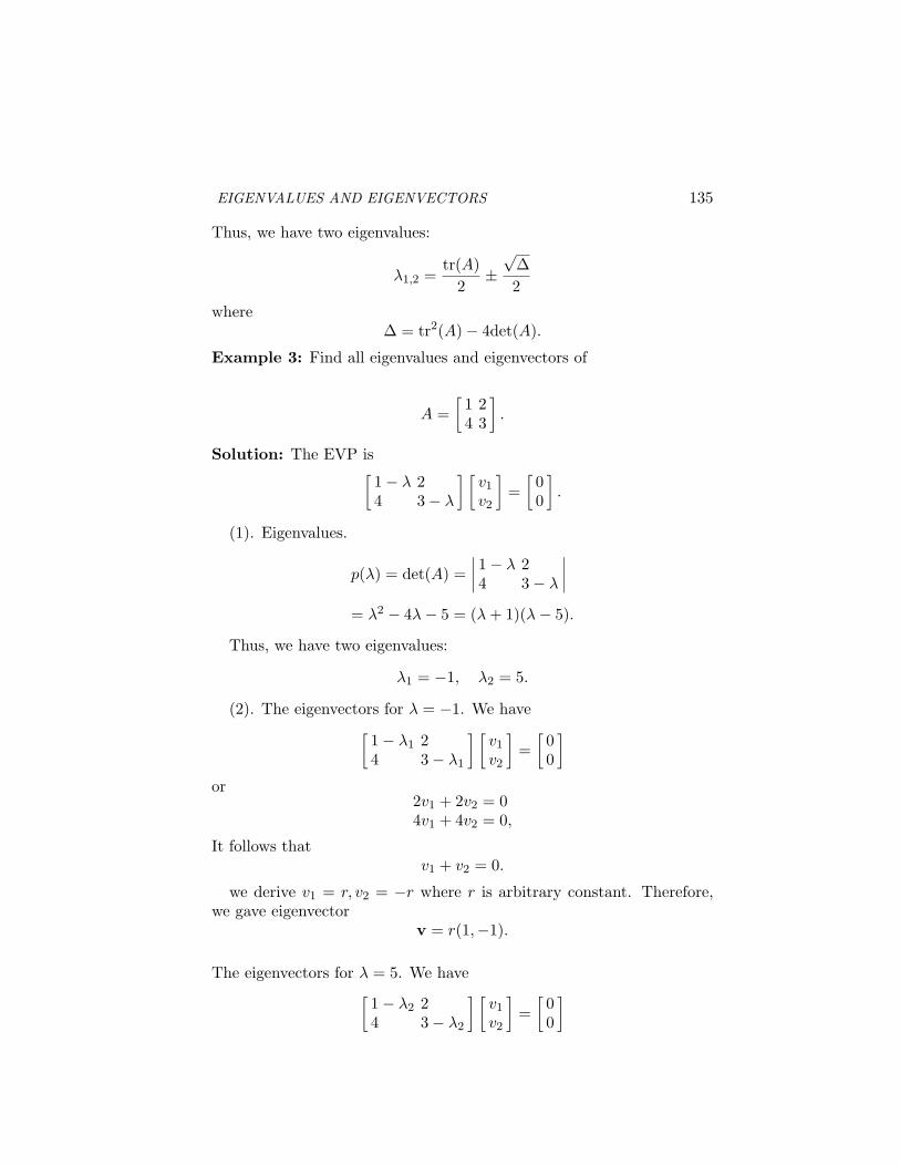
EIGENVALUES AND EIGENVECTORS 135
Thus, we have two eigenvalues:
λ1,2 =tr(A)
2±√
∆2
where∆ = tr2(A)− 4det(A).
Example 3: Find all eigenvalues and eigenvectors of
A =[1 24 3
].
Solution: The EVP is[1− λ 24 3− λ
] [v1
v2
]=
[00
].
(1). Eigenvalues.
p(λ) = det(A) =∣∣∣∣1− λ 24 3− λ
∣∣∣∣
= λ2 − 4λ− 5 = (λ + 1)(λ− 5).
Thus, we have two eigenvalues:
λ1 = −1, λ2 = 5.
(2). The eigenvectors for λ = −1. We have[1− λ1 24 3− λ1
] [v1
v2
]=
[00
]
or2v1 + 2v2 = 04v1 + 4v2 = 0,
It follows thatv1 + v2 = 0.
we derive v1 = r, v2 = −r where r is arbitrary constant. Therefore,we gave eigenvector
v = r(1,−1).
The eigenvectors for λ = 5. We have[1− λ2 24 3− λ2
] [v1
v2
]=
[00
]
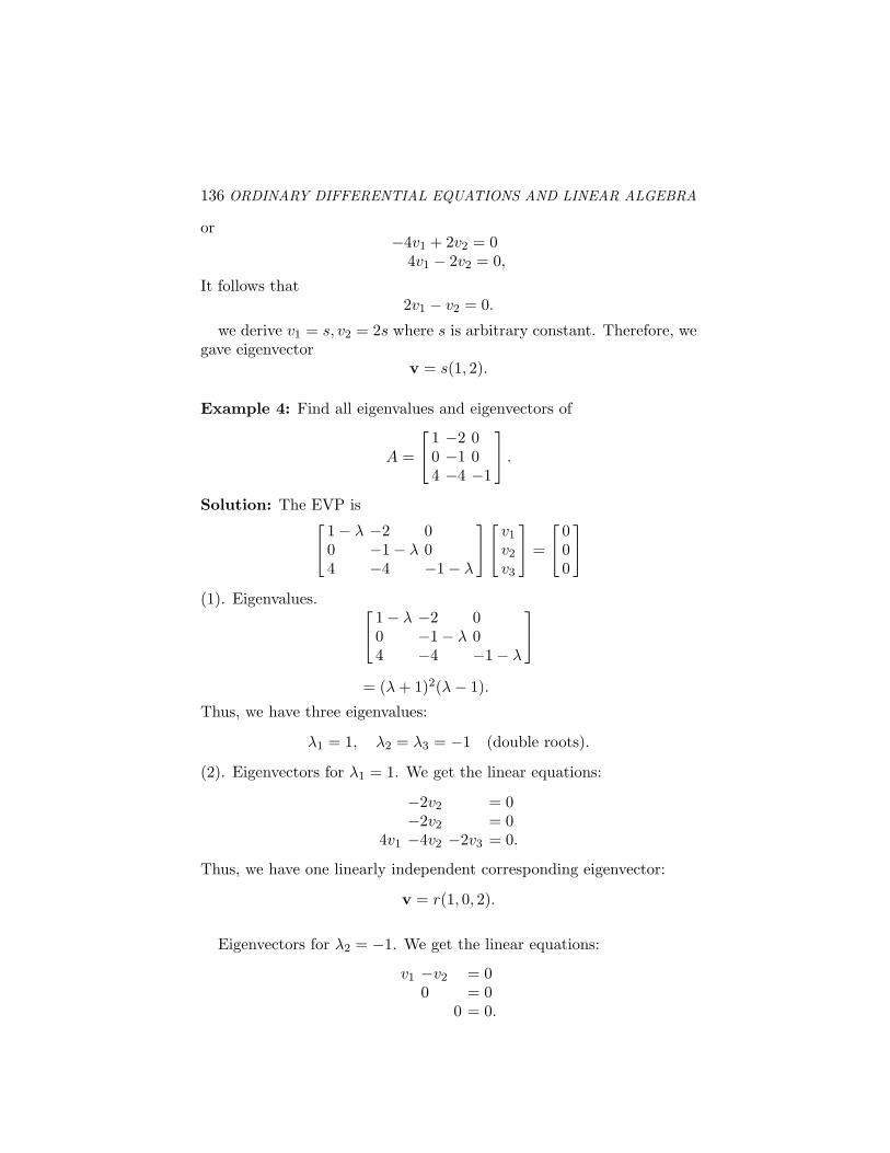
136 ORDINARY DIFFERENTIAL EQUATIONS AND LINEAR ALGEBRA
or−4v1 + 2v2 = 0
4v1 − 2v2 = 0,
It follows that2v1 − v2 = 0.
we derive v1 = s, v2 = 2s where s is arbitrary constant. Therefore, wegave eigenvector
v = s(1, 2).
Example 4: Find all eigenvalues and eigenvectors of
A =
1 −2 00 −1 04 −4 −1
.
Solution: The EVP is
1− λ −2 00 −1− λ 04 −4 −1− λ
v1
v2
v3
=
000
(1). Eigenvalues.
1− λ −2 00 −1− λ 04 −4 −1− λ
= (λ + 1)2(λ− 1).
Thus, we have three eigenvalues:
λ1 = 1, λ2 = λ3 = −1 (double roots).
(2). Eigenvectors for λ1 = 1. We get the linear equations:
−2v2 = 0−2v2 = 0
4v1 −4v2 −2v3 = 0.
Thus, we have one linearly independent corresponding eigenvector:
v = r(1, 0, 2).
Eigenvectors for λ2 = −1. We get the linear equations:
v1 −v2 = 00 = 0
0 = 0.
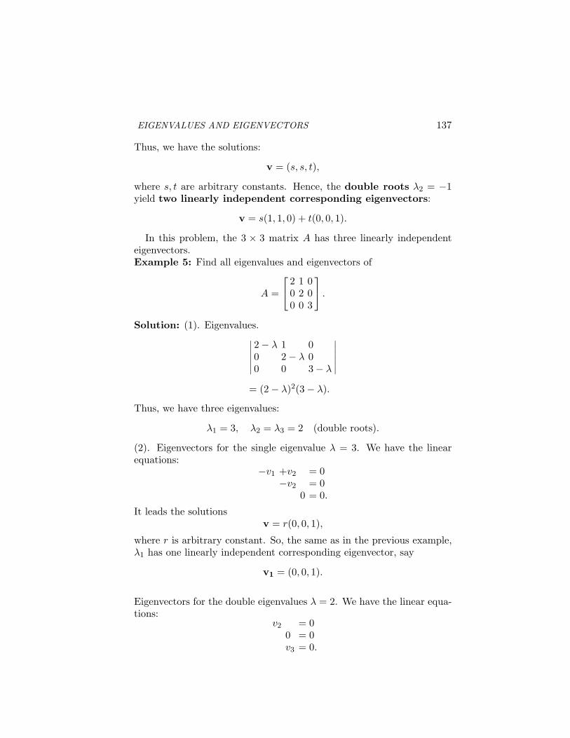
EIGENVALUES AND EIGENVECTORS 137
Thus, we have the solutions:
v = (s, s, t),
where s, t are arbitrary constants. Hence, the double roots λ2 = −1yield two linearly independent corresponding eigenvectors:
v = s(1, 1, 0) + t(0, 0, 1).
In this problem, the 3 × 3 matrix A has three linearly independenteigenvectors.Example 5: Find all eigenvalues and eigenvectors of
A =
2 1 00 2 00 0 3
.
Solution: (1). Eigenvalues.∣∣∣∣∣∣
2− λ 1 00 2− λ 00 0 3− λ
∣∣∣∣∣∣
= (2− λ)2(3− λ).
Thus, we have three eigenvalues:
λ1 = 3, λ2 = λ3 = 2 (double roots).
(2). Eigenvectors for the single eigenvalue λ = 3. We have the linearequations:
−v1 +v2 = 0−v2 = 0
0 = 0.
It leads the solutionsv = r(0, 0, 1),
where r is arbitrary constant. So, the same as in the previous example,λ1 has one linearly independent corresponding eigenvector, say
v1 = (0, 0, 1).
Eigenvectors for the double eigenvalues λ = 2. We have the linear equa-tions:
v2 = 00 = 0v3 = 0.
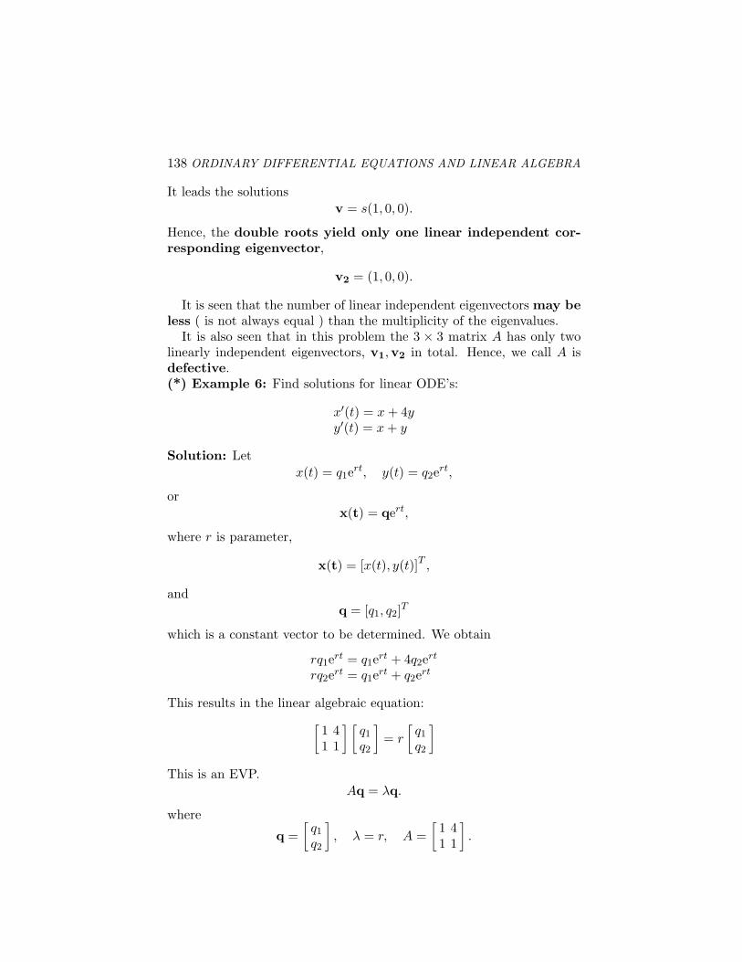
138 ORDINARY DIFFERENTIAL EQUATIONS AND LINEAR ALGEBRA
It leads the solutionsv = s(1, 0, 0).
Hence, the double roots yield only one linear independent cor-responding eigenvector,
v2 = (1, 0, 0).
It is seen that the number of linear independent eigenvectors may beless ( is not always equal ) than the multiplicity of the eigenvalues.
It is also seen that in this problem the 3 × 3 matrix A has only twolinearly independent eigenvectors, v1,v2 in total. Hence, we call A isdefective.(*) Example 6: Find solutions for linear ODE’s:
x′(t) = x + 4yy′(t) = x + y
Solution: Letx(t) = q1ert, y(t) = q2ert,
orx(t) = qert,
where r is parameter,
x(t) = [x(t), y(t)]T ,
andq = [q1, q2]T
which is a constant vector to be determined. We obtain
rq1ert = q1ert + 4q2ert
rq2ert = q1ert + q2ert
This results in the linear algebraic equation:[1 41 1
] [q1
q2
]= r
[q1
q2
]
This is an EVP.Aq = λq.
where
q =[q1
q2
], λ = r, A =
[1 41 1
].
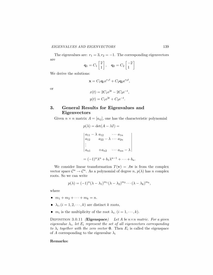
EIGENVALUES AND EIGENVECTORS 139
The eigenvalues are: r1 = 3, r2 = −1. The corresponding eigenvectorsare
q1 = C1
[21
], q2 = C2
[−21
]
We derive the solutions:
x = C1q1er1t + C2q2er2t,
orx(t) = 2C1e3t − 2C2e−t,
y(t) = C1e3t + C2e−t.
3. General Results for Eigenvalues andEigenvectors
Given n× n matrix A = [aij ], one has the characteristic polynomial
p(λ) = det(A− λI) =
∣∣∣∣∣∣∣∣∣
a11 − λ a12 · · · a1n
a12 a22 − λ · · · a2n...an1 +an2 · · · ann − λ
∣∣∣∣∣∣∣∣∣
= (−1)nλn + b1λn−1 + · · ·+ bn.
We consider linear transformation T (v) = Av is from the complexvector space Cn → Cn. As a polynomial of degree n, p(λ) has n complexroots. So we can write
p(λ) = (−1)n(λ− λ1)m1(λ− λ2)m2 · · · (λ− λk)mk ,
where
m1 + m2 + · · ·+ mk = n.
λi, (i = 1, 2, · · · , k) are distinct k roots,
mi is the multiplicity of the root λi, (i = 1, · · · , k).
Definition 3.0.11 (Eigenspace) Let A be n×n matric. For a giveneigenvalue λi, let Ei represent the set of all eigenvectors correspondingto λi together with the zero vector 0. Then Ei is called the eigenspaceof A corresponding to the eigenvalue λi
Remarks:
140 ORDINARY DIFFERENTIAL EQUATIONS AND LINEAR ALGEBRA
Eigenspace Ei of A must be a subspace of A. For example 5, corre-sponding to λ2 = 2,
E2 = {v ∈ R3 : v = s(1, 0, 0), s ∈ R}.while For example 4, corresponding to λ2 = −1,
E2 = {v ∈ R3 : v = s(1, 1, 0) + t(0, 0, 1), s, t ∈ R}.
Ei is the set of all solutions of the linear equations:
(A− λiI)v = 0.
or say,Ei = Ker{A− λI}.
Theorem 3.0.12 Let Ei is the eigenspace of A corresponding to mul-tiple eigenvalue λi with multiplicity mi. Let ni is the dimension of Ei,namely
ni = dim(Ei).
Then, we haveni ≤ mi.
Note: ni is the number of linearly independent eigenvectors correspond-ing to λi. We have previously shown by example that we may haveni < mi.
However, We did not show that ni > mi is impossible.
mi is called the algebraic multiplicity;
ni is called the geometric multiplicity;
The proof of the theorem is omitted.
Theorem 3.0.13 Eigenvectors corresponding to distinct eigenvaluesare linearly independent.
Proof: We adopt mathematical induction method to prove the result.Let {λ1, λ2, · · · , λm} be distinct eigenvalues of A, which has the corre-sponding eigenvectors:
{v1,v2, · · · ,vm}.
(1). For k = 1, {v1} is linearly independent.
EIGENVALUES AND EIGENVECTORS 141
(2). Assume that for k < m,
{v1,v2, · · · ,vk}are linearly independent. We consider
{v1,v2, · · · ,vk,vk+1}and wish to show they are also linearly independent.
(3). Let us to consider the linear combination:
u = {c1v1 + · · ·+ ckvk + ck+1vk+1} = 0. (9.2)
One derive that
Au = c1λ1v1 + c2λ2v2 + · · ·+ckλkvk + ck+1λk+1vk+1 = 0,
(9.3)
However, from (9.2), we have
ck+1vk+1 = −(c1v1 + c2v2 + · · ·+ ckvk),
then (9.3) is changed to
c1λ1v1 + c2λ2v2 + · · ·+ ckλkvk
−λk+1(c1v1 + c2v2 + · · ·+ ckvk) = 0,(9.4)
or
c1(λ1 − λk+1)v1 + c2(λ2 − λk+1)v2 + · · ·+ck(λk − λk+1)vk = 0,
(9.5)
However, as we assumed that
{v1,v2, · · · ,vk}are linearly independent, we derive
c1(λ1 − λk+1) = c2(λ2 − λk+1) = · · ·= ck(λk − λk+1) = 0.
Since λi are distinct, we derive
c1 = c2 = · · · = ck = 0.
142 ORDINARY DIFFERENTIAL EQUATIONS AND LINEAR ALGEBRA
Moreover, from (9.2), since vk+1 6= 0, we derive
ck+1 = 0.
Hence, we prove{v1,v2, · · · ,vk,vk+1}
are linear independent.
Definition 3.0.14 An n×n matrix A has n linearly independent eigen-vectors is said to have a complete set of eigenvectors, and we say A isnon-defective. If A does not have a complete set of eigenvectors, wesay A is defective.
Based on the above definition and theorem, it follows that
If A has n distinct eigenvalues, then it possess a complete set ofeigenvectors.
An n× n matrix A has a complete set of eigenvectors, if and only ifthe dimensions of each eigenspace is the same as the multiplicity ofthe corresponding eigenvalue. Namely,
ni = mi, for each i.
4. Symmetric MatricesSymmetric matrices (A = AT ) are very important type in applica-
tions. This type of matrices has important properties.
Theorem 4.0.15 (Real Eigenvalues) If A is symmetric , then alleigenvalues are real.Remark: If the eigenvalues are all real, the matrix A may be not sym-metric.
Proof: Omit.
Theorem 4.0.16 (Dimension of Eigen-space) If A is symmetricand λ is its eigenvalue of multiplicity k, then the eigen-space correspond-ing λ is of dimension k.
Proof: Omit.
Theorem 4.0.17 (Orthogonality of Eigenvectors) If A is sym-metric, then eigenvectors corresponding to distinct eigenvalues are or-thogonal.
EIGENVALUES AND EIGENVECTORS 143
Remark: If A is not symmetric, these eigenvectors are linearly inde-pendent, but they may be not orthogonal to each other.
Proof: Let thatAei = λiei, Aej = λjej .
Note that orthogonality of column vectors x,y ∈ Rm implies the dot(inner) product
x · y = 0.
However, the inner product can be calculated by the matrix multiplica-tion of column vectors in the form:
x · y = xTy.
Thus, we haveej · (Aei) = ej · (λiei),
so,eT
j Aei = λieTj ei
On the other hand, we have
(Aej) · ei = (λjej) · ei
so,(Aej)
Tei = (λjej)Tei.
This yields:eT
j ATei = λjeTj ei.
Since A = AT , we derive
0 = (λj − λi)eTj ei.
Due to (λj − λi) 6= 0, we prove
eTj ei = ej · ei = 0.
Theorem 4.0.18 (Orthogonality of Eigenvectors) If an n×n ma-trix A is symmetric, then its eigenvectors provides an orthogonal basisfor n-space.
Proof: We consider two cases separately.
1 All n eigenvalues are distinct. Then the system has n eigenvectorsorthogonal to each other. They form an orthogonal basis for then-space.
144 ORDINARY DIFFERENTIAL EQUATIONS AND LINEAR ALGEBRA
2 Suppose all eigenvalues are distinct, except one λ∗, which is of mul-tiplicity k. Then
the system has n− k simple eigenvalues, and n = k eigenvectors,which orthogonal to each other, as well orthogonal to all vectorsin the eigenspace S∗ corresponding to λ∗.
As dim(S∗) = k, it has an orthogonal basis with k vectors.
Thus, the system has a basis with (n− k)+ k = 0 orthogonal vectorsin total.
5. DiagonalizationA linear system with diagonal matrix is particularly easy to solve.
Especially for the case of very large n. In this case, the equations, like:
Ax = b,dxdt
= Ax, (9.6)
are uncoupled. Therefore, if A is not diagonal matrix, it is naturalto think that by introducing a variable transformation, such that thematrix of new problem becomes diagonal.
In doing so, Letx = Qv,
where Q is an invertible matrix. Then, (9.6) is changed to
Qdvdt
= AQv, (9.7)
or
dvdt
= Q−1AQv. (9.8)
If one can find a proper matrix Q such that
Q−1AQ = D =
d1 0 · · · 00 d2 · · · 0...0 0 · · · dn
then the new problem (9.8) can be easy to solve, and the solution oforiginal problem for x follows.
Theorem 5.0.19 (Diagonalization) Let A be n× n, then
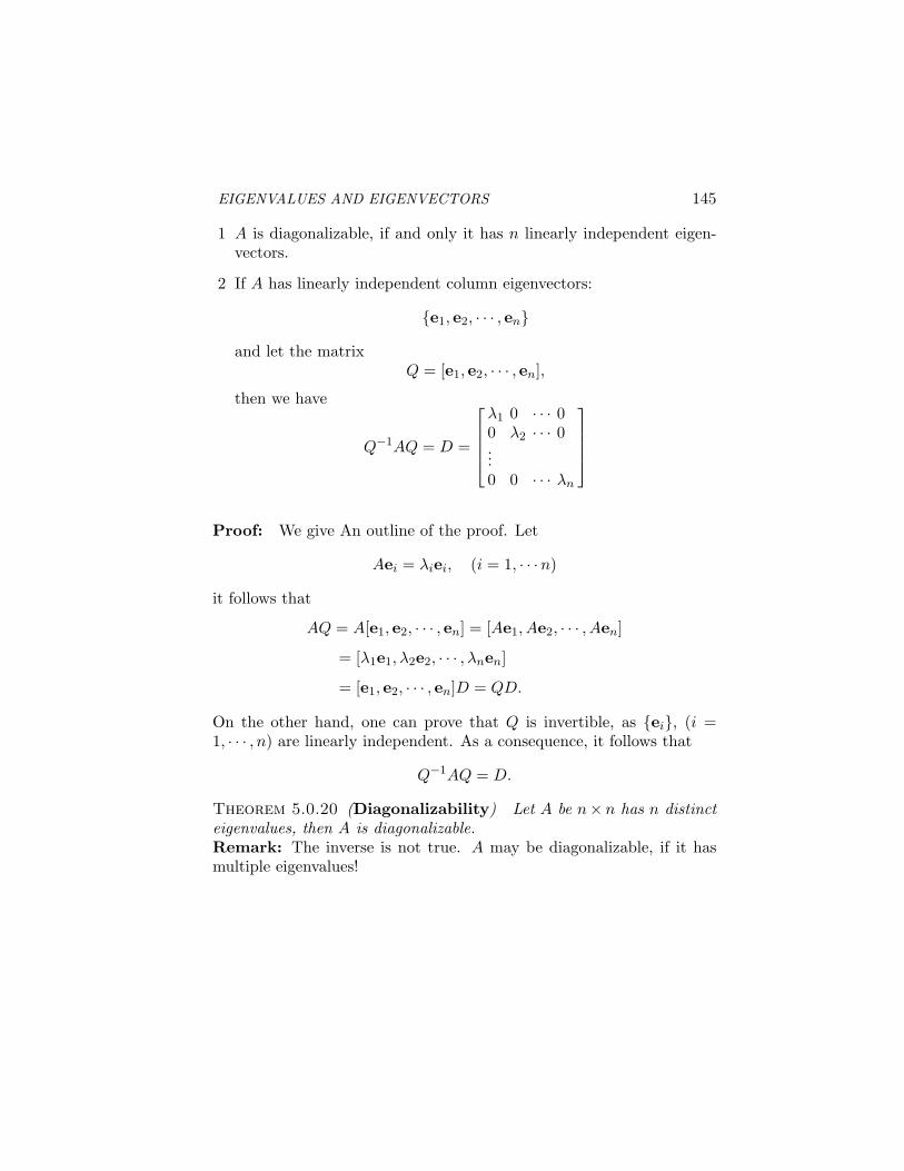
EIGENVALUES AND EIGENVECTORS 145
1 A is diagonalizable, if and only it has n linearly independent eigen-vectors.
2 If A has linearly independent column eigenvectors:
{e1, e2, · · · , en}and let the matrix
Q = [e1, e2, · · · , en],
then we have
Q−1AQ = D =
λ1 0 · · · 00 λ2 · · · 0...0 0 · · · λn
Proof: We give An outline of the proof. Let
Aei = λiei, (i = 1, · · ·n)
it follows that
AQ = A[e1, e2, · · · , en] = [Ae1, Ae2, · · · , Aen]
= [λ1e1, λ2e2, · · · , λnen]
= [e1, e2, · · · , en]D = QD.
On the other hand, one can prove that Q is invertible, as {ei}, (i =1, · · · , n) are linearly independent. As a consequence, it follows that
Q−1AQ = D.
Theorem 5.0.20 (Diagonalizability) Let A be n× n has n distincteigenvalues, then A is diagonalizable.Remark: The inverse is not true. A may be diagonalizable, if it hasmultiple eigenvalues!

Chapter 10
SYSTEMS OF LINEAR DIFFERENTIAL EQUATIONS:EIGENVECTOR METHOD
1. IntroductionIn this and the following lecture we will give an introduction to sys-
tems of differential equations. To start with, we consider a system oftwo first order equations is
dx1
dt= a11x1 + a12x2
dx2
dt= a21x1 + u22x2.
(10.1)
The system can be written in matrix form as
dudt
= Au
where
u =(
x1
x2
)
and
A =(
a11 a12
a21 a22
).
The problem of 2 × 2 system can be solved by transforming into asecond order equation. As matter of fact, we may discuss two cases:
Case (I): Assume a12 = 0.The first equation is decoupled from the second one:
dx1
dt= a11x1
dx2
dt= a21x1 + u22x2.
(10.2)
147
148 ORDINARY DIFFERENTIAL EQUATIONS AND LINEAR ALGEBRA
The system can be solved as 1-st order equations.
Case (II): Assume a12 6= 0.The first equation gives
x2 =1
a12
[dx1
dt− a11x1
].
Substituting this in the second equation and simplifying, we get 2-ndorder equation:
d2x1
dt2− tr(A)
dx1
dt+ det(A)x1 = 0. (10.3)
where tr(A) is the trace of A (sum of diagonal entries) and det(A) is thedeterminant of A, namely,
tr(A) = a11 + a22, det(A) =∣∣∣∣a11 a12
a21 a22
∣∣∣∣ .
As it is known that its solution has the form:
x1(t) = c1ert,
hence,x2(t) = c2ert.
The exponent r satisfy the characteristic equation:
φ(r) = r2 − tr(A)r + det(A) = 0. (10.4)
The characteristic polynomial in (10.4) has roots:
r1,2 =tr(A)±
√tr2(A)− 4det(A)
2.
If r1 6= r2, as we know that the general solution of this DE (10.3) is
x1(t) = c11er1t + c12e
r2t.
x2(t) = c21er1t + c22e
r2t.
wherec21/c11 =
1a12
[r1 − a11] ,
c22/c12 =1
a12[r2 − a11] .
EIGENVECTOR METHOD 149
Or, in the form of vector:
x = c1er1t + c2e
r2t. (10.5)
In general, one has a n × n system of equations, which can be writtenin the matrix form:
dxdt
= Ax
where column vector
x =
x1
x2...
xn
while
A =
a11 a12 · · · a1n
a21 a22 · · · a2n...
an1 an2 · · · ann
.
In general, a n × n system cannot be transformed in a n-th orderdifferential equation. in that case, the above elimination method is notapplicable. To find the solutions, we need to another way.
2. (n × n) System of Linear Equations andEigenvector Method
Let us consider the system
dxdt
= Ax. (10.6)
with an arbitrary n× n matrix A.Suppose that the solution can be written in the form:
x(t) = v eλt, (10.7)
where λ is a parameter, while
v = [v1, v2, · · · , vn]T
is a constant column vector, both are to be determined. Substituting(10.12) into (10.11), we derive
Av = λv,
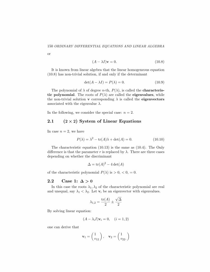
150 ORDINARY DIFFERENTIAL EQUATIONS AND LINEAR ALGEBRA
or
(A− λI)v = 0. (10.8)
It is known from linear algebra that the linear homogeneous equation(10.8) has non-trivial solution, if and only if the determinant
det(A− λI) = P (λ) = 0. (10.9)
The polynomial of λ of degree n-th, P (λ), is called the characteris-tic polynomial. The roots of P (λ) are called the eigenvalues, whilethe non-trivial solution v corresponding λ is called the eigenvectorsassociated with the eigenvalue λ.
In the following, we consider the special case: n = 2.
2.1 (2 × 2) System of Linear Equations
In case n = 2, we have
P (λ) = λ2 − tr(A)λ + det(A) = 0. (10.10)
The characteristic equation (10.13) is the same as (10.4). The Onlydifference is that the parameter r is replaced by λ. There are three casesdepending on whether the discriminant
∆ = tr(A)2 − 4 det(A)
of the characteristic polynomial P (λ) is > 0, < 0, = 0.
2.2 Case 1: ∆ > 0
In this case the roots λ1, λ2 of the characteristic polynomial are realand unequal, say λ1 < λ2. Let vi be an eigenvector with eigenvalues.
λ1,2 =tr(A)
2±√
∆2
By solving linear equation:
(A− λiI)vi = 0, (i = 1, 2)
one can derive that
v1 =(
1v12
), v2 =
(1v22.
)
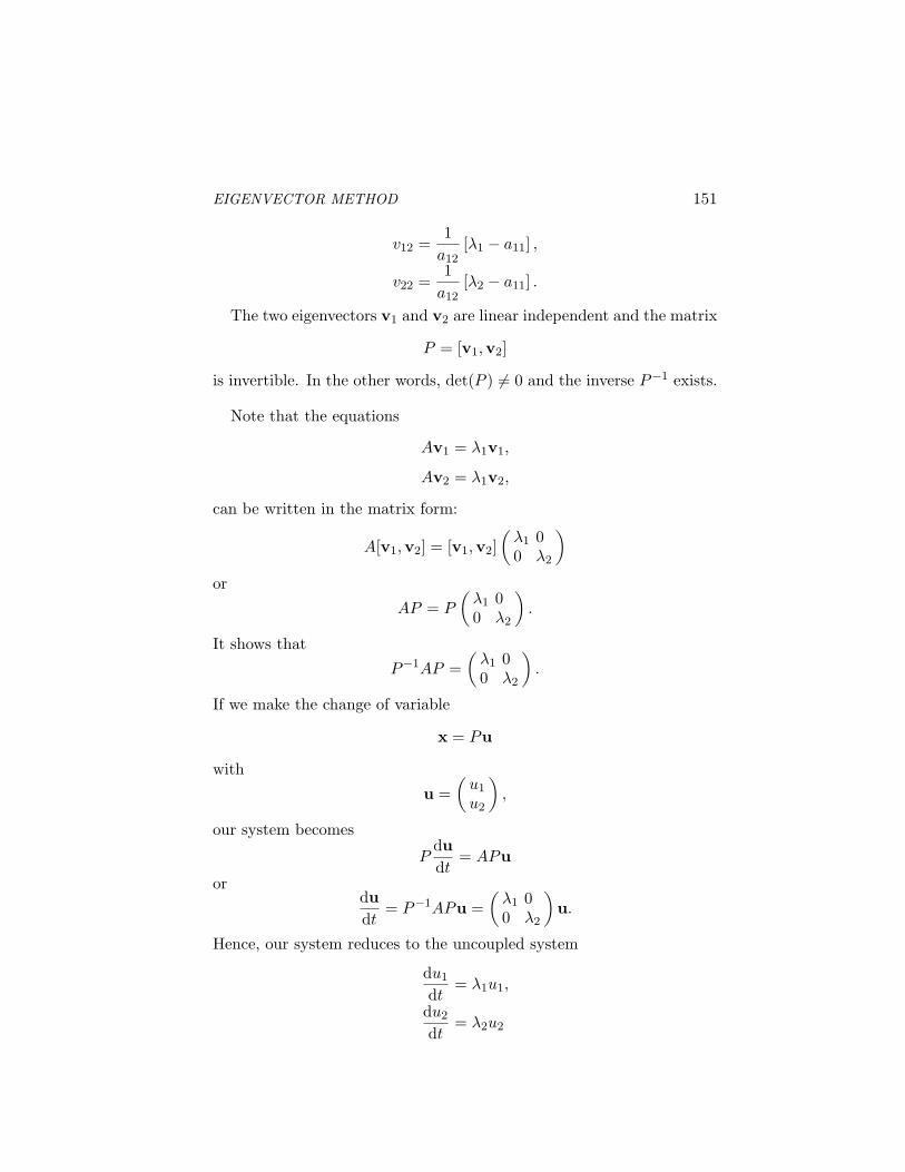
EIGENVECTOR METHOD 151
v12 =1
a12[λ1 − a11] ,
v22 =1
a12[λ2 − a11] .
The two eigenvectors v1 and v2 are linear independent and the matrix
P = [v1,v2]
is invertible. In the other words, det(P ) 6= 0 and the inverse P−1 exists.
Note that the equations
Av1 = λ1v1,
Av2 = λ1v2,
can be written in the matrix form:
A[v1,v2] = [v1,v2](
λ1 00 λ2
)
or
AP = P
(λ1 00 λ2
).
It shows that
P−1AP =(
λ1 00 λ2
).
If we make the change of variable
x = Pu
with
u =(
u1
u2
),
our system becomes
Pdudt
= APu
ordudt
= P−1APu =(
λ1 00 λ2
)u.
Hence, our system reduces to the uncoupled system
du1
dt= λ1u1,
du2
dt= λ2u2
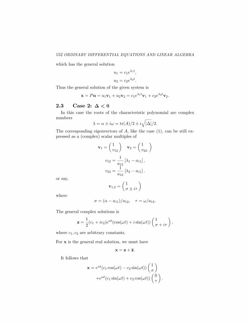
152 ORDINARY DIFFERENTIAL EQUATIONS AND LINEAR ALGEBRA
which has the general solution
u1 = c1eλ1t,
u2 = c2eλ2t.
Thus the general solution of the given system is
x = Pu = u1v1 + u2v2 = c1eλ1tv1 + c2e
λ2tv2.
2.3 Case 2: ∆ < 0
In this case the roots of the characteristic polynomial are complexnumbers
λ = α± iω = tr(A)/2± i√|∆|/2.
The corresponding eigenvectors of A, like the case (1), can be still ex-pressed as a (complex) scalar multiples of
v1 =(
1v12
)v2 =
(1v22.
)
v12 =1
a12[λ1 − a11] ,
v22 =1
a12[λ2 − a11] .
or say,
v1,2 =(
1σ ± iτ
)
whereσ = (α− a11)/a12, τ = ω/a12.
The general complex solutions is
z =12(c1 + ic2)eαt(cos(ωt) + i sin(ωt))
(1σ + iτ
),
where c1, c2 are arbitrary constants.
For x is the general real solution, we must have
x = z + z.
It follows that
x = eαt(c1 cos(ωt)− c2 sin(ωt))(
1σ
)
+eαt(c1 sin(ωt) + c2 cos(ωt))(
0τ
).
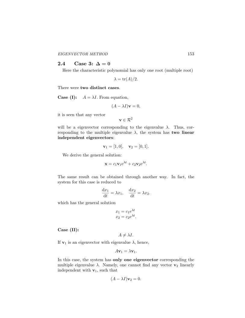
EIGENVECTOR METHOD 153
2.4 Case 3: ∆ = 0
Here the characteristic polynomial has only one root (multiple root)
λ = tr(A)/2.
There were two distinct cases.
Case (I): A = λI. From equation,
(A− λI)v = 0,
it is seen that any vectorv ∈ R2
will be a eigenvector corresponding to the eigenvalue λ. Thus, cor-responding to the multiple eigenvalue λ, the system has two linearindependent eigenvectors:
v1 = [1, 0], v2 = [0, 1].
We derive the general solution:
x = c1v1eλt + c2v2eλt.
The same result can be obtained through another way. In fact, thesystem for this case is reduced to
dx1
dt= λx1,
dx2
dt= λx2.
which has the general solution
x1 = c1eλt
x2 = c2eλt.
Case (II):A 6= λI.
If v1 is an eigenvector with eigenvalue λ, hence,
Av1 = λv1.
In this case, the system has only one eigenvector corresponding themultiple eigenvalue λ. Namely, one cannot find any vector v2 linearlyindependent with v1, such that
(A− λI)v2 = 0.
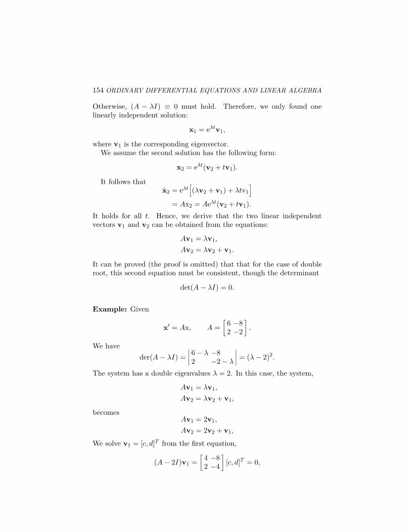
154 ORDINARY DIFFERENTIAL EQUATIONS AND LINEAR ALGEBRA
Otherwise, (A − λI) ≡ 0 must hold. Therefore, we only found onelinearly independent solution:
x1 = eλtv1,
where v1 is the corresponding eigenvector.We assume the second solution has the following form:
x2 = eλt(v2 + tv1).
It follows thatx2 = eλt
[(λv2 + v1) + λtv1
]
= Ax2 = Aeλt(v2 + tv1).
It holds for all t. Hence, we derive that the two linear independentvectors v1 and v2 can be obtained from the equations:
Av1 = λv1,
Av2 = λv2 + v1.
It can be proved (the proof is omitted) that that for the case of doubleroot, this second equation must be consistent, though the determinant
det(A− λI) = 0.
Example: Given
x′ = Ax, A =[6 −82 −2
].
We have
der(A− λI) =∣∣∣∣6− λ −82 −2− λ
∣∣∣∣ = (λ− 2)2.
The system has a double eigenvalues λ = 2. In this case, the system,
Av1 = λv1,
Av2 = λv2 + v1,
becomesAv1 = 2v1,
Av2 = 2v2 + v1,
We solve v1 = [c, d]T from the first equation,
(A− 2I)v1 =[4 −82 −4
][c, d]T = 0,
EIGENVECTOR METHOD 155
and obtainv1 = r[2, 1]T
the second equation for v2 = [a, b]T becomes
(A− 2I)v2 =[4 −82 −4
][a, b]T = r[2, 1]T .
It is seen that this equation is consistent and has the solutions:
v2 =[r
2+ 2s, s
],
where r, s are arbitrary constants. Let r = 2, s = 0, we get
v1 = [4, 2]T , v2 = [1, 0]T .
Note: For the case under discussion, one may introduce the matrix
P = [v1,v2],
we have
AP = P
(λ 10 λ
).
Since P is invertible, we may write
P−1AP =(
λ 10 λ
).
Setting as beforex = Pu
with
u =(
u1
u2
),
our system becomes
Pdudt
= APu
ordudt
= P−1APu =(
λ 10 λ
)u.
Hence, our system reduces to the uncoupled system
du1dt = λu1 + u2,
du2dt = λu2
156 ORDINARY DIFFERENTIAL EQUATIONS AND LINEAR ALGEBRA
which has the general solution
u2 = c2eλt,
u1 = c1eλt + c2teλt.
Thus the general solution of the given system is
x = Pu = u1v1 + u2v2
= (c1eλt + c2t)eλtv1 + c2eλtv2.
3. Stability of Solutions3.1 Definition of Stability
We now study the stability of the solutions for (2×2) system of linearequations:
dxdt
= Ax. (10.11)
with an arbitrary 2× 2 matrix A. Every solution
x(t) = {x1(t), x2(t)}can be geometrically described by a trajectory of moving point on thephase plane (x1, x2).
Definition 3.1.1 The constant solution x(t) = y(t) = 0 is called anequilibrium solution of our system.
This solution is said to be asymptotically stable if the generalsolution converges to it as t →∞.
A system is called stable if the trajectories are all bounded ast →∞.
A system is called unstable if it is not stable. Hence, some of thetrajectories must be unbounded as t →∞.
As we have known, the solution can be derived in the form:
x(t) = v eλt, (10.12)
where the eigenvalue λ satisfies the characteristic equation:
P (λ) = λ2 − tr(A)λ + det(A) = 0. (10.13)
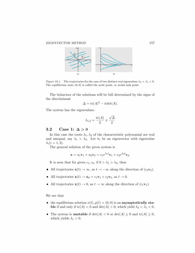
EIGENVECTOR METHOD 157
Figure 10.1. The trajectories for the case of two distinct real eigenvalues λ2 < λ1 < 0.The equilibrium state (0, 0) is called the node point, or nodal sink point
The behaviors of the solutions will be full determined by the signs ofthe discriminant
∆ = tr(A)2 − 4 det(A).
The system has the eigenvalues:
λ1,2 =tr(A)
2±√
∆2
3.2 Case 1: ∆ > 0
In this case the roots λ1, λ2 of the characteristic polynomial are realand unequal, say λ1 > λ2. Let vi be an eigenvector with eigenvalueλi(i = 1, 2).
The general solution of the given system is
x = u1v1 + u2v2 = c1eλ1tv1 + c2e
λ2tv2.
It is seen that for given c1, c2, if 0 > λ1 > λ2, then
All trajectories x(t) →∞, as t → −∞ along the direction of (c2v2).
All trajectories x(t) → x0 = c1v1 + c2v2, as t → 0.
All trajectories x(t) → 0, as t →∞ along the direction of (c1v1).
We see that
the equilibrium solution x(t), y(t) = (0, 0) is an asymptotically sta-ble if and only if tr(A) < 0 and det(A) > 0, which yield λ2 < λ1 < 0.
The system is unstable if det(A) < 0 or det(A) ≥ 0 and tr(A) ≥ 0,which yields λ1 > 0.
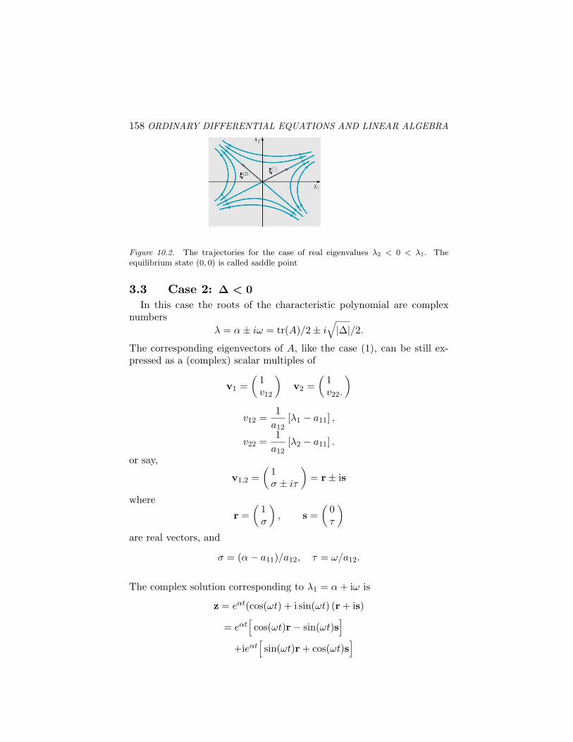
158 ORDINARY DIFFERENTIAL EQUATIONS AND LINEAR ALGEBRA
Figure 10.2. The trajectories for the case of real eigenvalues λ2 < 0 < λ1. Theequilibrium state (0, 0) is called saddle point
3.3 Case 2: ∆ < 0
In this case the roots of the characteristic polynomial are complexnumbers
λ = α± iω = tr(A)/2± i√|∆|/2.
The corresponding eigenvectors of A, like the case (1), can be still ex-pressed as a (complex) scalar multiples of
v1 =(
1v12
)v2 =
(1v22.
)
v12 =1
a12[λ1 − a11] ,
v22 =1
a12[λ2 − a11] .
or say,
v1,2 =(
1σ ± iτ
)= r± is
where
r =(
1σ
), s =
(0τ
)
are real vectors, and
σ = (α− a11)/a12, τ = ω/a12.
The complex solution corresponding to λ1 = α + iω is
z = eαt(cos(ωt) + i sin(ωt) (r + is)
= eαt[cos(ωt)r− sin(ωt)s
]
+ieαt[sin(ωt)r + cos(ωt)s
]
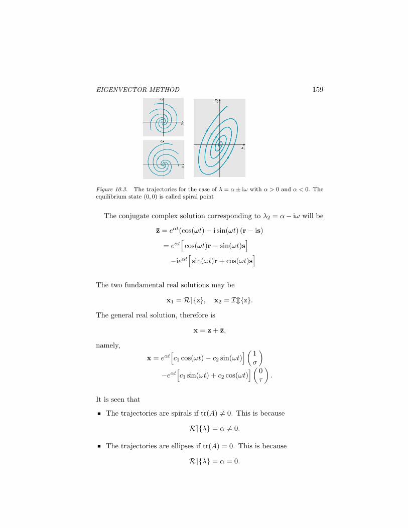
EIGENVECTOR METHOD 159
Figure 10.3. The trajectories for the case of λ = α± iω with α > 0 and α < 0. Theequilibrium state (0, 0) is called spiral point
The conjugate complex solution corresponding to λ2 = α− iω will be
z = eαt(cos(ωt)− i sin(ωt) (r− is)
= eαt[cos(ωt)r− sin(ωt)s
]
−ieαt[sin(ωt)r + cos(ωt)s
]
The two fundamental real solutions may be
x1 = Re{z}, x2 = Im{z}.The general real solution, therefore is
x = z + z,
namely,
x = eαt[c1 cos(ωt)− c2 sin(ωt)
] (1σ
)
−eαt[c1 sin(ωt) + c2 cos(ωt)
] (0τ
).
It is seen that
The trajectories are spirals if tr(A) 6= 0. This is because
Re{λ} = α 6= 0.
The trajectories are ellipses if tr(A) = 0. This is because
Re{λ} = α = 0.
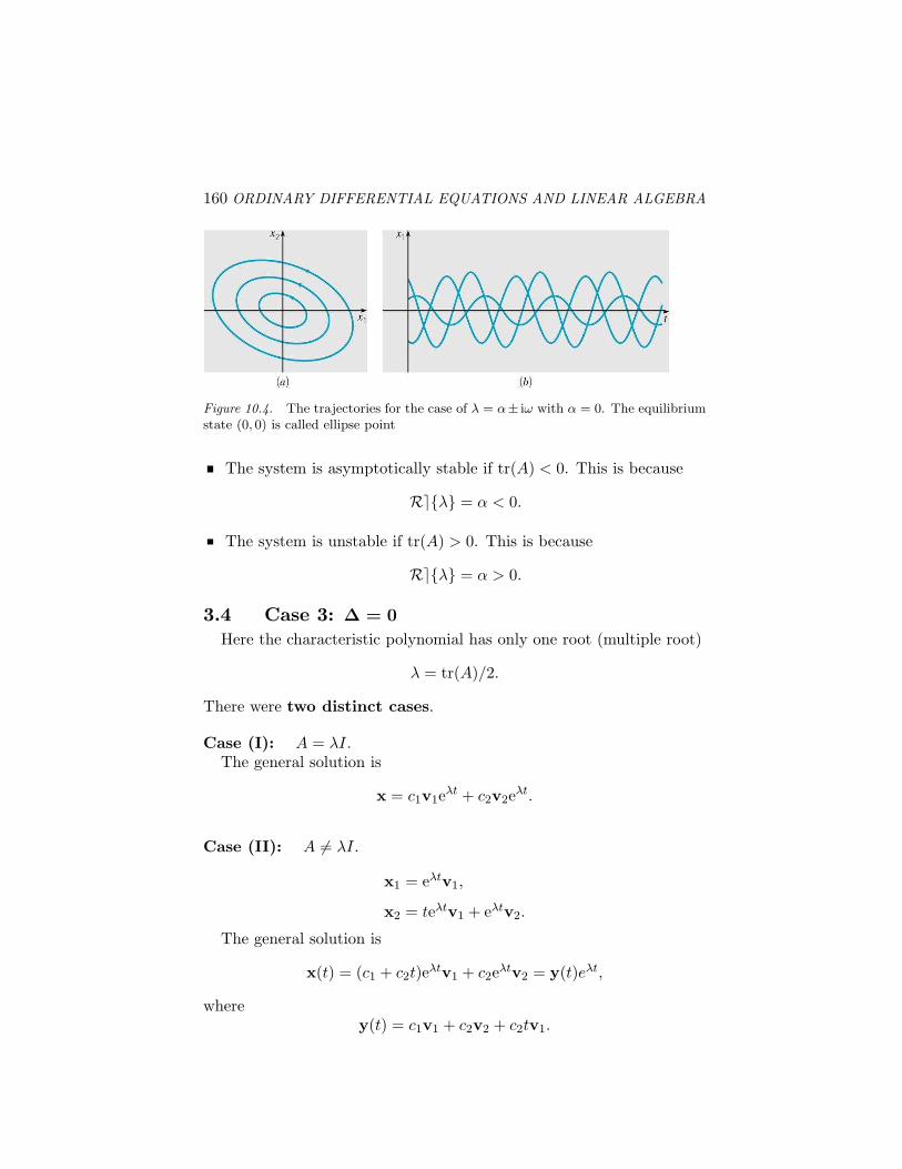
160 ORDINARY DIFFERENTIAL EQUATIONS AND LINEAR ALGEBRA
Figure 10.4. The trajectories for the case of λ = α± iω with α = 0. The equilibriumstate (0, 0) is called ellipse point
The system is asymptotically stable if tr(A) < 0. This is because
Re{λ} = α < 0.
The system is unstable if tr(A) > 0. This is because
Re{λ} = α > 0.
3.4 Case 3: ∆ = 0
Here the characteristic polynomial has only one root (multiple root)
λ = tr(A)/2.
There were two distinct cases.
Case (I): A = λI.The general solution is
x = c1v1eλt + c2v2eλt.
Case (II): A 6= λI.
x1 = eλtv1,
x2 = teλtv1 + eλtv2.
The general solution is
x(t) = (c1 + c2t)eλtv1 + c2eλtv2 = y(t)eλt,
wherey(t) = c1v1 + c2v2 + c2tv1.
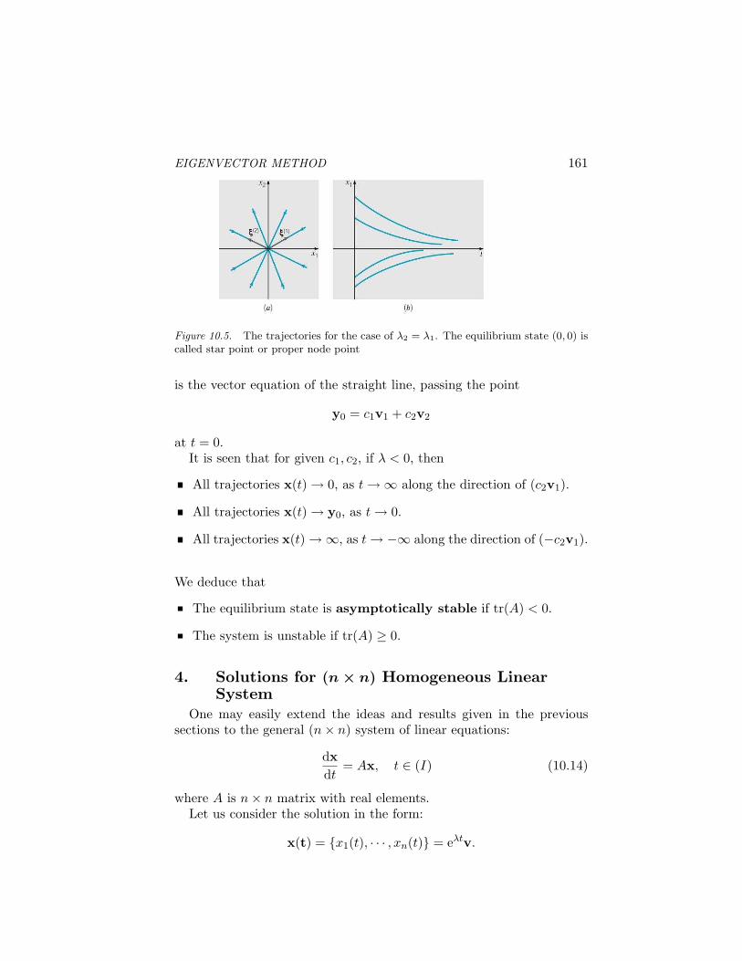
EIGENVECTOR METHOD 161
Figure 10.5. The trajectories for the case of λ2 = λ1. The equilibrium state (0, 0) iscalled star point or proper node point
is the vector equation of the straight line, passing the point
y0 = c1v1 + c2v2
at t = 0.It is seen that for given c1, c2, if λ < 0, then
All trajectories x(t) → 0, as t →∞ along the direction of (c2v1).
All trajectories x(t) → y0, as t → 0.
All trajectories x(t) →∞, as t → −∞ along the direction of (−c2v1).
We deduce that
The equilibrium state is asymptotically stable if tr(A) < 0.
The system is unstable if tr(A) ≥ 0.
4. Solutions for (n × n) Homogeneous LinearSystem
One may easily extend the ideas and results given in the previoussections to the general (n× n) system of linear equations:
dxdt
= Ax, t ∈ (I) (10.14)
where A is n× n matrix with real elements.Let us consider the solution in the form:
x(t) = {x1(t), · · · , xn(t)} = eλtv.
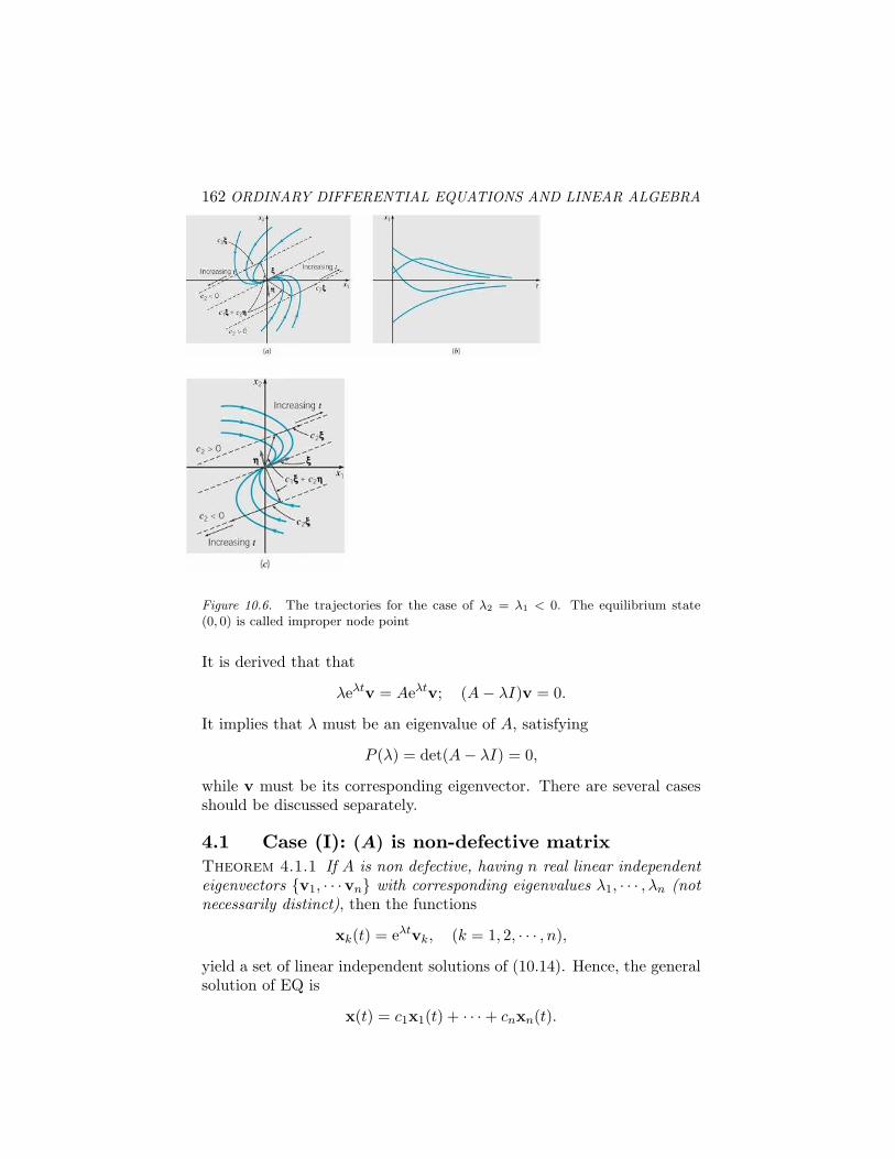
162 ORDINARY DIFFERENTIAL EQUATIONS AND LINEAR ALGEBRA
Figure 10.6. The trajectories for the case of λ2 = λ1 < 0. The equilibrium state(0, 0) is called improper node point
It is derived that that
λeλtv = Aeλtv; (A− λI)v = 0.
It implies that λ must be an eigenvalue of A, satisfying
P (λ) = det(A− λI) = 0,
while v must be its corresponding eigenvector. There are several casesshould be discussed separately.
4.1 Case (I): (A) is non-defective matrixTheorem 4.1.1 If A is non defective, having n real linear independenteigenvectors {v1, · · ·vn} with corresponding eigenvalues λ1, · · · , λn (notnecessarily distinct), then the functions
xk(t) = eλtvk, (k = 1, 2, · · · , n),
yield a set of linear independent solutions of (10.14). Hence, the generalsolution of EQ is
x(t) = c1x1(t) + · · ·+ cnxn(t).
EIGENVECTOR METHOD 163
Proof: We have just shown that xk(t) are solution. So, we only need toprove the n vector functions are linear independent. This can be doneby shown their determinant
det[x1, · · ·xn] = e(λ1+···+λn)t det[v1, · · · ,vn] 6= 0,
for all t ∈ (I).
Example 1: Find the general solution for EQ x′ = Ax with
A =
0 2 −3−2 4 −3−2 2 −1
.
solution: It is calculated that
P (λ) = −(λ + 1)(λ− 2)2,
so that A has simple EV λ = −1 and double EV λ = 2. We now proceedto find the corresponding eigenvectors.
For λ1 = −1, we solve the system:
v1 + 2v2 − 3v3 = 0,−2v1 + 5v2 − 3v3 = 0−2v1 + 2v2 = 0.
It yields the solution v = (v1, v2, v3) = r(1, 1, 1), where r is arbitraryconstant. Thus, we have the corresponding eigenvector
v1 = (1, 1, 1).
For λ2 = 2, the multiplicity is m2 = 2, the system may reduce to asingle EQ:
2v1 − 2v2 + 3v3 = 0,
which has the general solution v = r(1, 1, 0) + s(−3, 0, 2), where r, sare arbitrary constants. Thus, we have the two corresponding eigen-vectors
v2 = (1, 1, 0), v3 = (−3, 0, 2).The dimension of eigen-space E2 is n2 = dim(E2) = 2.
Thus, the system is non-defective, we have three L.I. solutions:
x1 = e−t(1, 1, 1)T ;x2 = e2t(1, 1, 0)T ;x3 = e2t(−3, 0, 2)T .
The general solution is
x(t) = c1x1(t) + c2x2(t) + c3x3(t).
164 ORDINARY DIFFERENTIAL EQUATIONS AND LINEAR ALGEBRA
4.2 Case (II): (A) has a pair of complexconjugate eigen-values
Theorem 4.2.1 If A has a pair of complex conjugate EV’s, (λ, λ) =a ± ib, with corresponding complex conjugate eigenvector are (v, v) =vR ± ivI, then the functions
x1(t) = eat[cos(bt)vR − sin(bt)vI
],
x2(t) = eat[sin(bt)vR + cos(bt)vI
],
yield a pair of linear independent real solutions of (10.14).
Proof: The theorem for case (I) is applicable for the complex EV. Hence,the system has a pair of the complex solutions:
x(t) = eλtv; x(t) = eλtv.
Taking real part and imaginary part, respectively, we obtain the realsolutions:
x1(t) = <{x(t)}; x2(t) = ={x(t)}.
4.3 Case (III): (A) is a defective matrixTheorem 4.3.1 Assume that A is defective with multiple eigenvalue λwith the multiplicity m ≥ 1; the dimension of the eigen-space dim(E) =k < m, and the corresponding the eigenvectors in the eigen-space are(v1, · · ·vk). Then beside of solutions given by these eigenvectors:
xi(t) = eλtvi, (i = 1, 2, · · · k).
one may look for the following forms (m− k) solutions for the system:
x1(t) = eλt[v1,0 + tv1,1
],
x2(t) = eλt[v2,0 + tv2,1 + t2
2! v2,2
],
...xj(t) = eλt
[vj,0 + tvj,1 + · · ·+ tj
j! vj,j
],
...(j = 1, 2, · · ·m− k).
To determine the vectors {vj,i, (i = 0, 1, · · · j)}, we may substitutexj(t) into EQ (10.14):
x′j(t) = λeλt[vj,0 + tvj,1 + · · ·+ tj
j! vj,j
]
+eλt[vj,1 + tvj,2 + · · ·+ tj−1
(j−1)! vj,j
]
= Aeλt[vj,0 + tvj,1 + · · ·+ tj
j! vj,j
].
EIGENVECTOR METHOD 165
It holds for all t ∈ (I). Equating the coefficients of each power term oft of both sides, if follows that
(A− λI)vj,j = 0,(A− λI)vj,j−1 = vj,j
(A− λI)vj,j−2 = vj,j−1...
(A− λI)vj,0 = vj,1.
(10.15)
It is seen that vj,j is one of the eigenvector corresponding to λ. It canbe proved that the system (10.15) allows a set of non-zero solutions{vj,i, (i = 0, 1, · · · j)}.The whole set of solutions {xi(t); xj(t)} yield m linear independent so-lutions of (10.14).
We do not give the proof of the above statement, but show the ideasvia the following example.
Example 2: Find the general solution for EQ: x′ = Ax with
A =
6 3 61 4 2−2 −2 −1
.
Solution: It is calculate that P (λ) = (λ − 3)3. One has EV, λ = 3,multiplicity m = 3. The corresponding eigenvectors v = r(−1, 1, 0) +s(−2, 0, 1), where (r, s) are two arbitrary constants. Hence, we havev1 = (−1, 1, 0)T ; v2 = (−2, 0, 1)T , and dim(E) = k = 2 < m. (A) isdefective matrix. Thus, we have two solutions:
x1(t) = e3tv1; x2(t) = e3tv2.
The third solution can be expressed in the form:
x1(t) = e3t(v1 + tv2),
where (v1; v2) are subject to the system:
(A− 3I)v1 = 0,(A− 3I)v0 = v1.
(10.16)
It is seen that v1 = r(−1, 1, 0) + s(−2, 0, 1), r, s are to be determined.Furthermore, let us denote v0 = (a, b, c)T . (10.16) can be written as
3a + 3b + 6c = −r − 2sa + b + c = r−2a− 2b− 4c = s
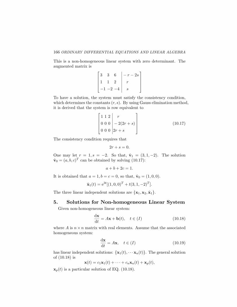
166 ORDINARY DIFFERENTIAL EQUATIONS AND LINEAR ALGEBRA
This is a non-homogeneous linear system with zero determinant. Theaugmented matrix is
3 3 6∣∣∣− r − 2s
1 1 2∣∣∣ r
−1 −2 −4∣∣∣ s
To have a solution, the system must satisfy the consistency condition,which determines the constants (r, s). By using Gauss elimination method,it is derived that the system is row equivalent to
1 1 2∣∣∣ r
0 0 0∣∣∣− 2(2r + s)
0 0 0∣∣∣2r + s
(10.17)
The consistency condition requires that
2r + s = 0.
One may let r = 1, s = −2. So that, v1 = (3, 1,−2). The solutionv0 = (a, b, c)T can be obtained by solving (10.17):
a + b + 2c = 1.
It is obtained that a = 1, b = c = 0, so that, v0 = (1, 0, 0).
x1(t) = e3t[(1, 0, 0)T + t(3, 1,−2)T ].
The three linear independent solutions are {x1,x2, x1}.
5. Solutions for Non-homogeneous Linear SystemGiven non-homogeneous linear system:
dxdt
= Ax + b(t), t ∈ (I) (10.18)
where A is n×n matrix with real elements. Assume that the associatedhomogeneous system:
dxdt
= Ax, t ∈ (I) (10.19)
has linear independent solutions: {x1(t), · · ·xn(t)}. The general solutionof (10.18) is
x(t) = c1x1(t) + · · ·+ cnxn(t) + xp(t),
xp(t) is a particular solution of EQ. (10.18).
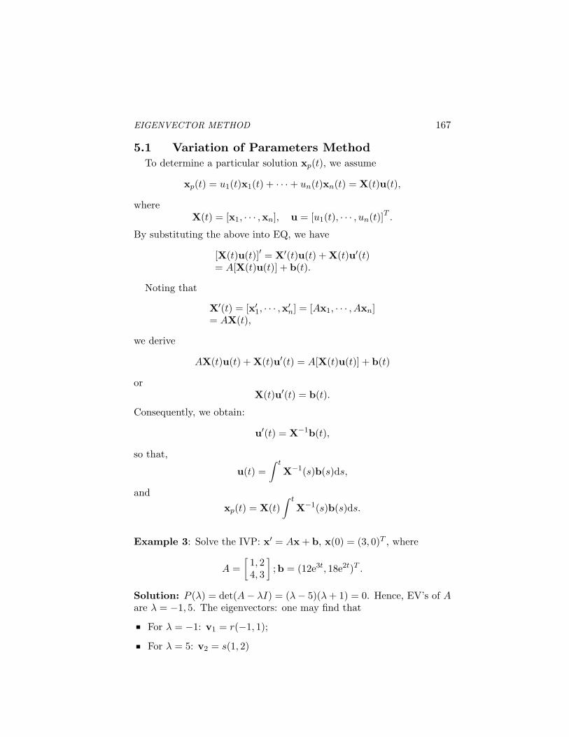
EIGENVECTOR METHOD 167
5.1 Variation of Parameters MethodTo determine a particular solution xp(t), we assume
xp(t) = u1(t)x1(t) + · · ·+ un(t)xn(t) = X(t)u(t),
whereX(t) = [x1, · · · ,xn], u = [u1(t), · · · , un(t)]T .
By substituting the above into EQ, we have
[X(t)u(t)]′ = X′(t)u(t) + X(t)u′(t)= A[X(t)u(t)] + b(t).
Noting that
X′(t) = [x′1, · · · ,x′n] = [Ax1, · · · , Axn]= AX(t),
we derive
AX(t)u(t) + X(t)u′(t) = A[X(t)u(t)] + b(t)
orX(t)u′(t) = b(t).
Consequently, we obtain:
u′(t) = X−1b(t),
so that,
u(t) =∫ t
X−1(s)b(s)ds,
andxp(t) = X(t)
∫ t
X−1(s)b(s)ds.
Example 3: Solve the IVP: x′ = Ax + b, x(0) = (3, 0)T , where
A =[1, 24, 3
];b = (12e3t, 18e2t)T .
Solution: P (λ) = det(A− λI) = (λ− 5)(λ + 1) = 0. Hence, EV’s of Aare λ = −1, 5. The eigenvectors: one may find that
For λ = −1: v1 = r(−1, 1);
For λ = 5: v2 = s(1, 2)
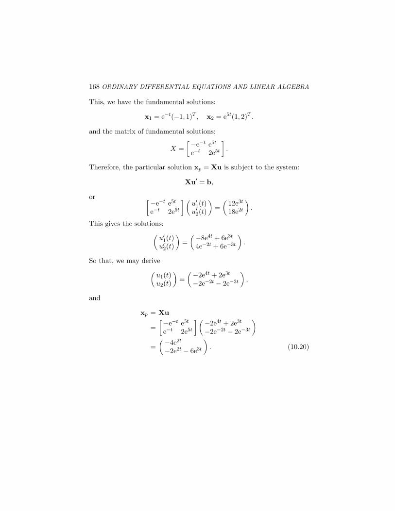
168 ORDINARY DIFFERENTIAL EQUATIONS AND LINEAR ALGEBRA
This, we have the fundamental solutions:
x1 = e−t(−1, 1)T , x2 = e5t(1, 2)T .
and the matrix of fundamental solutions:
X =[−e−t e5t
e−t 2e5t
].
Therefore, the particular solution xp = Xu is subject to the system:
Xu′ = b,
or [−e−t e5t
e−t 2e5t
] (u′1(t)u′2(t)
)=
(12e3t
18e2t
).
This gives the solutions:(
u′1(t)u′2(t)
)=
(−8e4t + 6e3t
4e−2t + 6e−3t
).
So that, we may derive(
u1(t)u2(t)
)=
(−2e4t + 2e3t
−2e−2t − 2e−3t
),
and
xp = Xu
=[−e−t e5t
e−t 2e5t
] (−2e4t + 2e3t
−2e−2t − 2e−3t
)
=(−4e2t
−2e2t − 6e3t
). (10.20)
Appendix AASSIGNMENTS AND SOLUTIONS
169
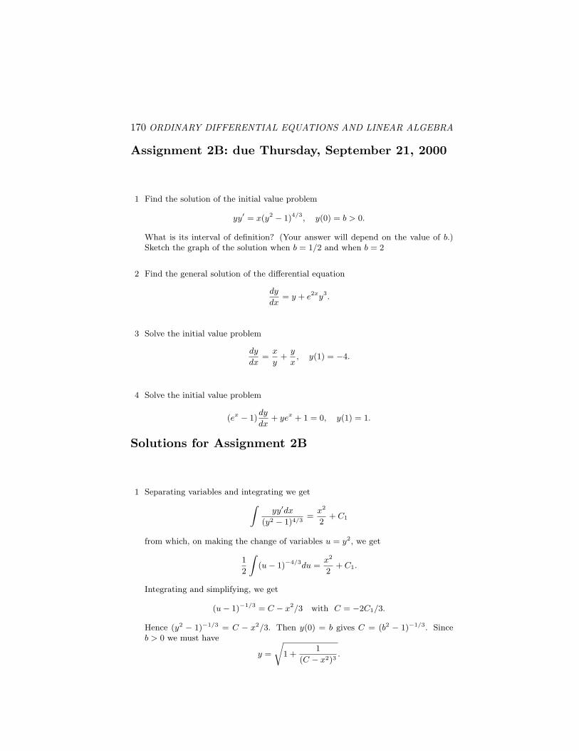
170 ORDINARY DIFFERENTIAL EQUATIONS AND LINEAR ALGEBRA
Assignment 2B: due Thursday, September 21, 2000
1 Find the solution of the initial value problem
yy′ = x(y2 − 1)4/3, y(0) = b > 0.
What is its interval of definition? (Your answer will depend on the value of b.)Sketch the graph of the solution when b = 1/2 and when b = 2
2 Find the general solution of the differential equation
dy
dx= y + e2xy3.
3 Solve the initial value problem
dy
dx=
x
y+
y
x, y(1) = −4.
4 Solve the initial value problem
(ex − 1)dy
dx+ yex + 1 = 0, y(1) = 1.
Solutions for Assignment 2B
1 Separating variables and integrating we get
∫yy′dx
(y2 − 1)4/3=
x2
2+ C1
from which, on making the change of variables u = y2, we get
1
2
∫(u− 1)−4/3du =
x2
2+ C1.
Integrating and simplifying, we get
(u− 1)−1/3 = C − x2/3 with C = −2C1/3.
Hence (y2 − 1)−1/3 = C − x2/3. Then y(0) = b gives C = (b2 − 1)−1/3. Sinceb > 0 we must have
y =
√1 +
1
(C − x2)3.
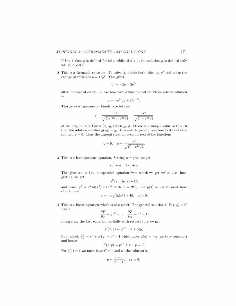
APPENDIX A: ASSIGNMENTS AND SOLUTIONS 171
If b < 1 then y is defined for all x while, if b > 1, the solution y is defined onlyfor |x| < √
3C.
2 This is a Bernoulli equation. To solve it, divide both sides by y3 and make thechange of variables u = 1/y2. This gives
u′ = −2u− 2e2x
after multiplication by −2. We now have a linear equation whose general solutionis
u = −e2x/2 + Ce−2x.
This gives a 1-parameter family of solutions
y =±1√
Ce−2x − e2x/2=
±ex
√C − e4x/2
of the original DE. Given (x0, y0) with y0 6= 0 there is a unique value of C suchthat the solution satisfies y(x0) = y0. It is not the general solution as it omits thesolution y = 0. Thus the general solution is comprised of the functions
y = 0, y =±ex
√C − e4x/2
.
3 This is a homogeneous equation. Setting u = y/x, we get
xu′ + u = 1/u + u.
This gives xu′ = 1/u, a separable equation from which we get uu′ = 1/x. Inte-grating, we get
u2/2 = ln |x|+ C1
and hence y2 = x2 ln(x2) + Cx2 with C = 2C1. For y(1) = −4 we must haveC = 16 and
y = −x√
ln(x2) + 16, x > 0.
4 This is a linear equation which is also exact. The general solution is F (x, y) = Cwhere
∂F
∂x= yex − 1,
∂F
∂y= ey − 1.
Integrating the first equation partially with respect to x we get
F (x, y) = yex + x + φ(y)
from which ∂F∂y
= ex + φ′(y) = ey − 1 which gives φ(y) = −y (up to a constant)and hence
F (x, y) = yex + x− y = C.
For y(1) = 1 we must have C = e and so the solution is
y =e− x
ex − 1, (x > 0).
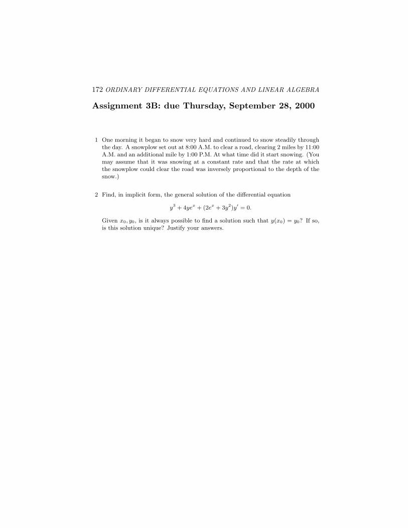
172 ORDINARY DIFFERENTIAL EQUATIONS AND LINEAR ALGEBRA
Assignment 3B: due Thursday, September 28, 2000
1 One morning it began to snow very hard and continued to snow steadily throughthe day. A snowplow set out at 8:00 A.M. to clear a road, clearing 2 miles by 11:00A.M. and an additional mile by 1:00 P.M. At what time did it start snowing. (Youmay assume that it was snowing at a constant rate and that the rate at whichthe snowplow could clear the road was inversely proportional to the depth of thesnow.)
2 Find, in implicit form, the general solution of the differential equation
y3 + 4yex + (2ex + 3y2)y′ = 0.
Given x0, y0, is it always possible to find a solution such that y(x0) = y0? If so,is this solution unique? Justify your answers.
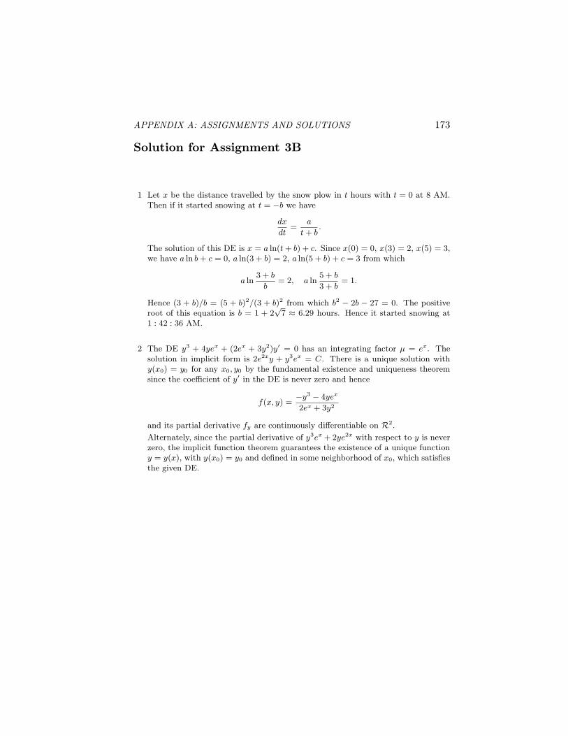
APPENDIX A: ASSIGNMENTS AND SOLUTIONS 173
Solution for Assignment 3B
1 Let x be the distance travelled by the snow plow in t hours with t = 0 at 8 AM.Then if it started snowing at t = −b we have
dx
dt=
a
t + b.
The solution of this DE is x = a ln(t + b) + c. Since x(0) = 0, x(3) = 2, x(5) = 3,we have a ln b + c = 0, a ln(3 + b) = 2, a ln(5 + b) + c = 3 from which
a ln3 + b
b= 2, a ln
5 + b
3 + b= 1.
Hence (3 + b)/b = (5 + b)2/(3 + b)2 from which b2 − 2b − 27 = 0. The positiveroot of this equation is b = 1 + 2
√7 ≈ 6.29 hours. Hence it started snowing at
1 : 42 : 36 AM.
2 The DE y3 + 4yex + (2ex + 3y2)y′ = 0 has an integrating factor µ = ex. Thesolution in implicit form is 2e2xy + y3ex = C. There is a unique solution withy(x0) = y0 for any x0, y0 by the fundamental existence and uniqueness theoremsince the coefficient of y′ in the DE is never zero and hence
f(x, y) =−y3 − 4yex
2ex + 3y2
and its partial derivative fy are continuously differentiable on R2.
Alternately, since the partial derivative of y3ex + 2ye2x with respect to y is neverzero, the implicit function theorem guarantees the existence of a unique functiony = y(x), with y(x0) = y0 and defined in some neighborhood of x0, which satisfiesthe given DE.
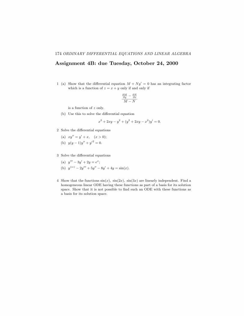
174 ORDINARY DIFFERENTIAL EQUATIONS AND LINEAR ALGEBRA
Assignment 4B: due Tuesday, October 24, 2000
1 (a) Show that the differential equation M + Ny′ = 0 has an integrating factorwhich is a function of z = x + y only if and only if
∂M∂y
− ∂N∂x
M −N
is a function of z only.
(b) Use this to solve the differential equation
x2 + 2xy − y2 + (y2 + 2xy − x2)y′ = 0.
2 Solve the differential equations
(a) xy′′ = y′ + x, (x > 0);
(b) y(y − 1)y′′ + y′2 = 0.
3 Solve the differential equations
(a) y′′′ − 3y′ + 2y = ex;
(b) y(iv) − 2y′′′ + 5y′′ − 8y′ + 4y = sin(x).
4 Show that the functions sin(x), sin(2x), sin(3x) are linearly independent. Find ahomogeneous linear ODE having these functions as part of a basis for its solutionspace. Show that it is not possible to find such an ODE with these functions asa basis for its solution space.
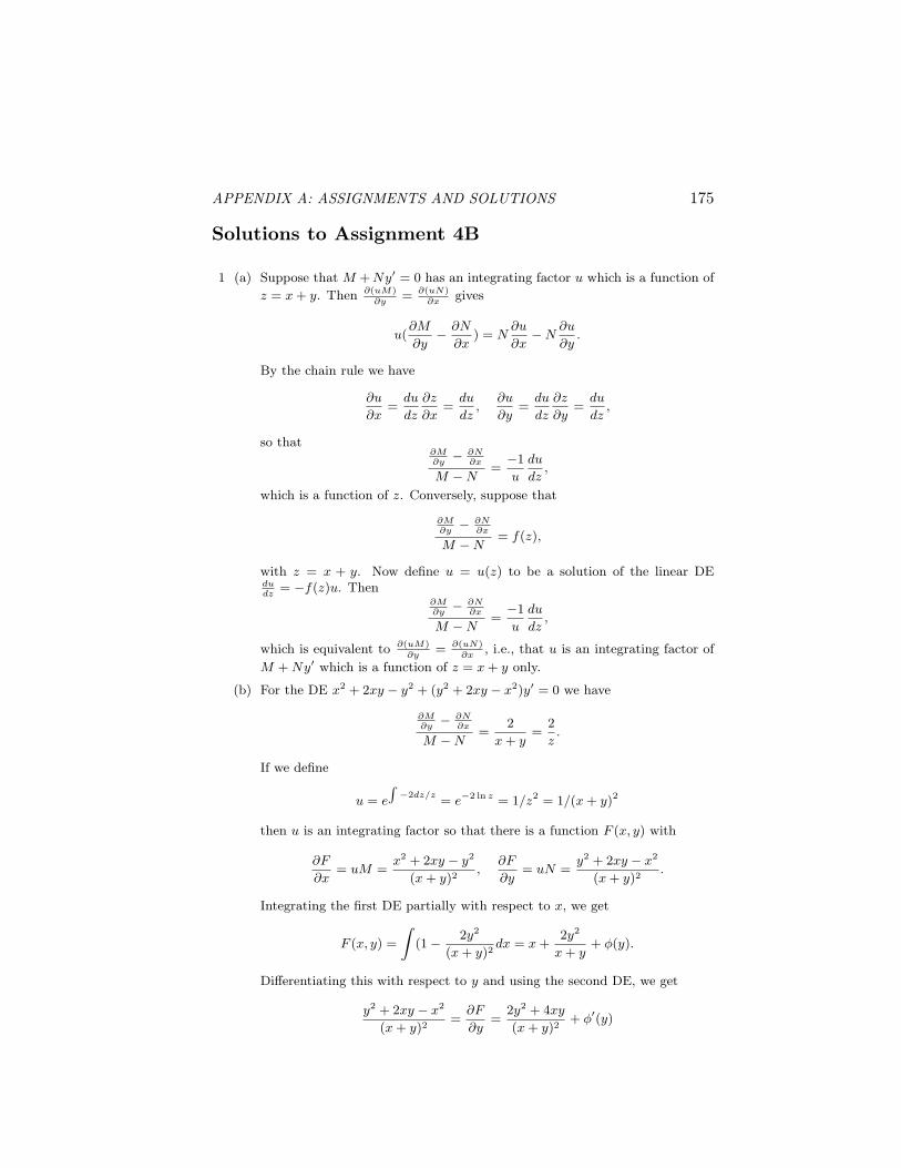
APPENDIX A: ASSIGNMENTS AND SOLUTIONS 175
Solutions to Assignment 4B
1 (a) Suppose that M + Ny′ = 0 has an integrating factor u which is a function of
z = x + y. Then ∂(uM)∂y
= ∂(uN)∂x
gives
u(∂M
∂y− ∂N
∂x) = N
∂u
∂x−N
∂u
∂y.
By the chain rule we have
∂u
∂x=
du
dz
∂z
∂x=
du
dz,
∂u
∂y=
du
dz
∂z
∂y=
du
dz,
so that∂M∂y
− ∂N∂x
M −N=−1
u
du
dz,
which is a function of z. Conversely, suppose that
∂M∂y
− ∂N∂x
M −N= f(z),
with z = x + y. Now define u = u(z) to be a solution of the linear DEdudz
= −f(z)u. Then∂M∂y
− ∂N∂x
M −N=−1
u
du
dz,
which is equivalent to ∂(uM)∂y
= ∂(uN)∂x
, i.e., that u is an integrating factor of
M + Ny′ which is a function of z = x + y only.
(b) For the DE x2 + 2xy − y2 + (y2 + 2xy − x2)y′ = 0 we have
∂M∂y
− ∂N∂x
M −N=
2
x + y=
2
z.
If we define
u = e
∫−2dz/z
= e−2 ln z = 1/z2 = 1/(x + y)2
then u is an integrating factor so that there is a function F (x, y) with
∂F
∂x= uM =
x2 + 2xy − y2
(x + y)2,
∂F
∂y= uN =
y2 + 2xy − x2
(x + y)2.
Integrating the first DE partially with respect to x, we get
F (x, y) =
∫(1− 2y2
(x + y)2dx = x +
2y2
x + y+ φ(y).
Differentiating this with respect to y and using the second DE, we get
y2 + 2xy − x2
(x + y)2=
∂F
∂y=
2y2 + 4xy
(x + y)2+ φ′(y)
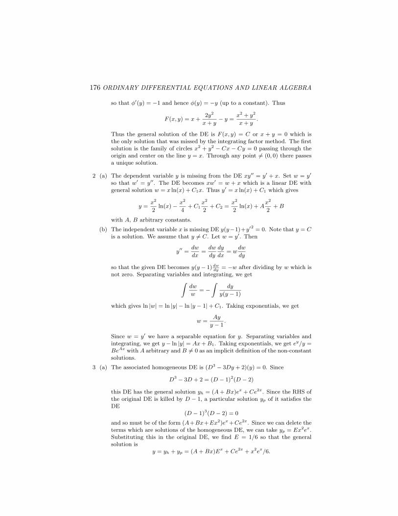
176 ORDINARY DIFFERENTIAL EQUATIONS AND LINEAR ALGEBRA
so that φ′(y) = −1 and hence φ(y) = −y (up to a constant). Thus
F (x, y) = x +2y2
x + y− y =
x2 + y2
x + y.
Thus the general solution of the DE is F (x, y) = C or x + y = 0 which isthe only solution that was missed by the integrating factor method. The firstsolution is the family of circles x2 + y2 − Cx − Cy = 0 passing through theorigin and center on the line y = x. Through any point 6= (0, 0) there passesa unique solution.
2 (a) The dependent variable y is missing from the DE xy′′ = y′ + x. Set w = y′
so that w′ = y′′. The DE becomes xw′ = w + x which is a linear DE withgeneral solution w = x ln(x) + C1x. Thus y′ = x ln(x) + C1 which gives
y =x2
2ln(x)− x2
4+ C1
x2
2+ C2 =
x2
2ln(x) + A
x2
2+ B
with A, B arbitrary constants.
(b) The independent variable x is missing DE y(y−1)+y′2 = 0. Note that y = Cis a solution. We assume that y 6= C. Let w = y′. Then
y′′ =dw
dx=
dw
dy
dy
dx= w
dw
dy
so that the given DE becomes y(y− 1) dwdy
= −w after dividing by w which isnot zero. Separating variables and integrating, we get
∫dw
w= −
∫dy
y(y − 1)
which gives ln |w| = ln |y| − ln |y − 1|+ C1. Taking exponentials, we get
w =Ay
y − 1.
Since w = y′ we have a separable equation for y. Separating variables andintegrating, we get y− ln |y| = Ax + B1. Taking exponentials, we get ey/y =BeAx with A arbitrary and B 6= 0 as an implicit definition of the non-constantsolutions.
3 (a) The associated homogeneous DE is (D3 − 3Dy + 2)(y) = 0. Since
D3 − 3D + 2 = (D − 1)2(D − 2)
this DE has the general solution yh = (A + Bx)ex + Ce2x. Since the RHS ofthe original DE is killed by D − 1, a particular solution yp of it satisfies theDE
(D − 1)3(D − 2) = 0
and so must be of the form (A+Bx+Ex2)ex +Ce2x. Since we can delete theterms which are solutions of the homogeneous DE, we can take yp = Ex2ex.Substituting this in the original DE, we find E = 1/6 so that the generalsolution is
y = yh + yp = (A + Bx)Ex + Ce2x + x2ex/6.
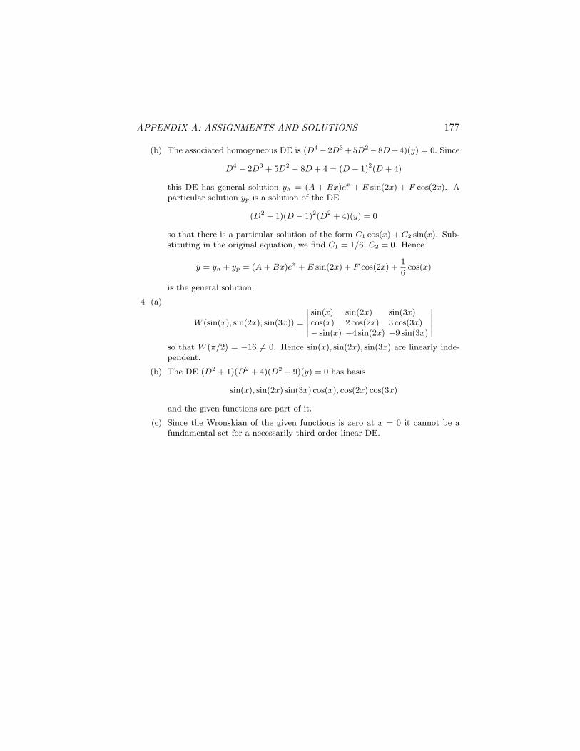
APPENDIX A: ASSIGNMENTS AND SOLUTIONS 177
(b) The associated homogeneous DE is (D4− 2D3 +5D2− 8D +4)(y) = 0. Since
D4 − 2D3 + 5D2 − 8D + 4 = (D − 1)2(D + 4)
this DE has general solution yh = (A + Bx)ex + E sin(2x) + F cos(2x). Aparticular solution yp is a solution of the DE
(D2 + 1)(D − 1)2(D2 + 4)(y) = 0
so that there is a particular solution of the form C1 cos(x) + C2 sin(x). Sub-stituting in the original equation, we find C1 = 1/6, C2 = 0. Hence
y = yh + yp = (A + Bx)ex + E sin(2x) + F cos(2x) +1
6cos(x)
is the general solution.
4 (a)
W (sin(x), sin(2x), sin(3x)) =
∣∣∣∣∣sin(x) sin(2x) sin(3x)cos(x) 2 cos(2x) 3 cos(3x)− sin(x) −4 sin(2x) −9 sin(3x)
∣∣∣∣∣so that W (π/2) = −16 6= 0. Hence sin(x), sin(2x), sin(3x) are linearly inde-pendent.
(b) The DE (D2 + 1)(D2 + 4)(D2 + 9)(y) = 0 has basis
sin(x), sin(2x) sin(3x) cos(x), cos(2x) cos(3x)
and the given functions are part of it.
(c) Since the Wronskian of the given functions is zero at x = 0 it cannot be afundamental set for a necessarily third order linear DE.
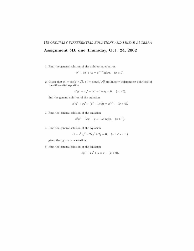
178 ORDINARY DIFFERENTIAL EQUATIONS AND LINEAR ALGEBRA
Assignment 5B: due Thursday, Oct. 24, 2002
1 Find the general solution of the differential equation
y′′ + 4y′ + 4y = e−2x ln(x), (x > 0).
2 Given that y1 = cos(x)/√
x, y2 = sin(x)/√
x are linearly independent solutions ofthe differential equation
x2y′′ + xy′ + (x2 − 1/4)y = 0, (x > 0),
find the general solution of the equation
x2y′′ + xy′ + (x2 − 1/4)y = x5/2, (x > 0).
3 Find the general solution of the equation
x2y′′ + 3xy′ + y = 1/x ln(x), (x > 0).
4 Find the general solution of the equation
(1− x2)y′′ − 2xy′ + 2y = 0, (−1 < x < 1)
given that y = x is a solution.
5 Find the general solution of the equation
xy′′ + xy′ + y = x, (x > 0).
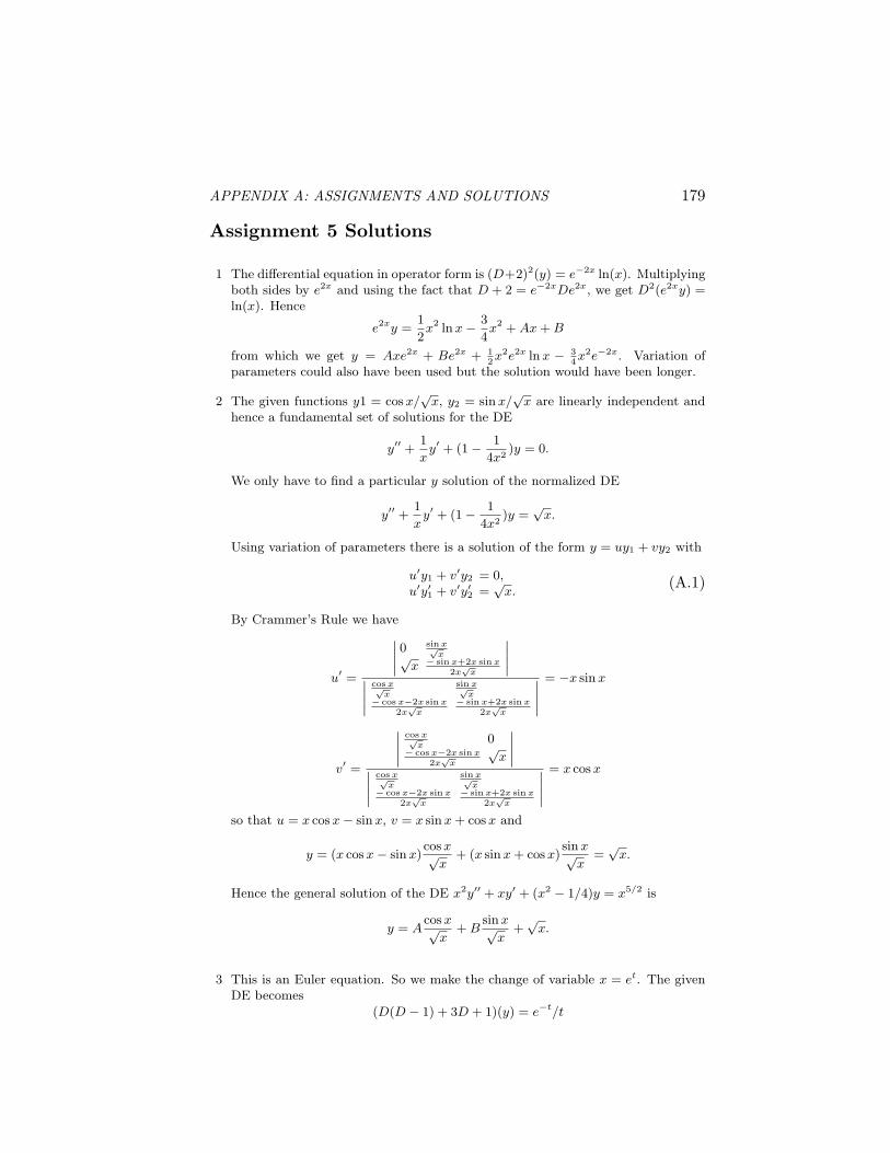
APPENDIX A: ASSIGNMENTS AND SOLUTIONS 179
Assignment 5 Solutions
1 The differential equation in operator form is (D+2)2(y) = e−2x ln(x). Multiplyingboth sides by e2x and using the fact that D + 2 = e−2xDe2x, we get D2(e2xy) =ln(x). Hence
e2xy =1
2x2 ln x− 3
4x2 + Ax + B
from which we get y = Axe2x + Be2x + 12x2e2x ln x − 3
4x2e−2x. Variation of
parameters could also have been used but the solution would have been longer.
2 The given functions y1 = cos x/√
x, y2 = sin x/√
x are linearly independent andhence a fundamental set of solutions for the DE
y′′ +1
xy′ + (1− 1
4x2)y = 0.
We only have to find a particular y solution of the normalized DE
y′′ +1
xy′ + (1− 1
4x2)y =
√x.
Using variation of parameters there is a solution of the form y = uy1 + vy2 with
u′y1 + v′y2 = 0,u′y′1 + v′y′2 =
√x.
(A.1)
By Crammer’s Rule we have
u′ =
∣∣∣∣0 sin x√
x√x − sin x+2x sin x
2x√
x
∣∣∣∣∣∣∣∣
cos x√x
sin x√x
− cos x−2x sin x2x√
x− sin x+2x sin x
2x√
x
∣∣∣∣= −x sin x
v′ =
∣∣∣∣cos x√
x0
− cos x−2x sin x2x√
x
√x
∣∣∣∣∣∣∣∣
cos x√x
sin x√x
− cos x−2x sin x2x√
x− sin x+2x sin x
2x√
x
∣∣∣∣= x cos x
so that u = x cos x− sin x, v = x sin x + cos x and
y = (x cos x− sin x)cos x√
x+ (x sin x + cos x)
sin x√x
=√
x.
Hence the general solution of the DE x2y′′ + xy′ + (x2 − 1/4)y = x5/2 is
y = Acos x√
x+ B
sin x√x
+√
x.
3 This is an Euler equation. So we make the change of variable x = et. The givenDE becomes
(D(D − 1) + 3D + 1)(y) = e−t/t
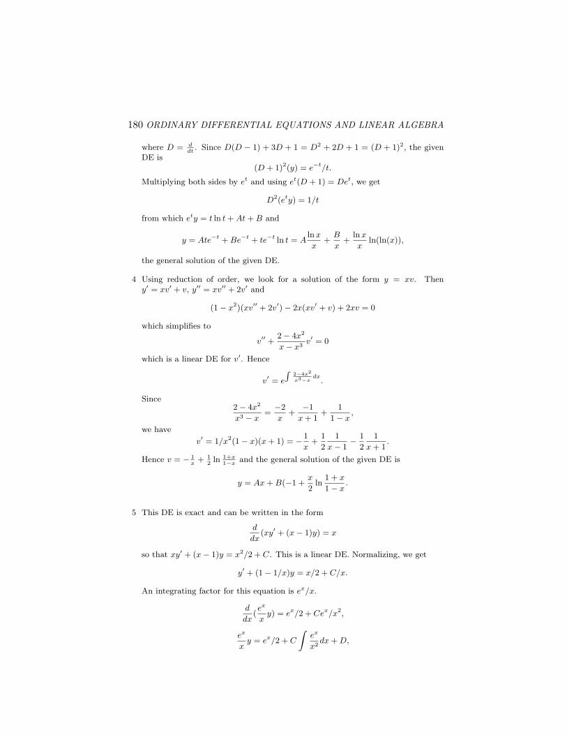
180 ORDINARY DIFFERENTIAL EQUATIONS AND LINEAR ALGEBRA
where D = ddt
. Since D(D − 1) + 3D + 1 = D2 + 2D + 1 = (D + 1)2, the givenDE is
(D + 1)2(y) = e−t/t.
Multiplying both sides by et and using et(D + 1) = Det, we get
D2(ety) = 1/t
from which ety = t ln t + At + B and
y = Ate−t + Be−t + te−t ln t = Aln x
x+
B
x+
ln x
xln(ln(x)),
the general solution of the given DE.
4 Using reduction of order, we look for a solution of the form y = xv. Theny′ = xv′ + v, y′′ = xv′′ + 2v′ and
(1− x2)(xv′′ + 2v′)− 2x(xv′ + v) + 2xv = 0
which simplifies to
v′′ +2− 4x2
x− x3v′ = 0
which is a linear DE for v′. Hence
v′ = e
∫2−4x2
x3−xdx
.
Since2− 4x2
x3 − x=−2
x+
−1
x + 1+
1
1− x,
we have
v′ = 1/x2(1− x)(x + 1) = − 1
x+
1
2
1
x− 1− 1
2
1
x + 1.
Hence v = − 1x
+ 12
ln 1+x1−x
and the general solution of the given DE is
y = Ax + B(−1 +x
2ln
1 + x
1− x.
5 This DE is exact and can be written in the form
d
dx(xy′ + (x− 1)y) = x
so that xy′ + (x− 1)y = x2/2 + C. This is a linear DE. Normalizing, we get
y′ + (1− 1/x)y = x/2 + C/x.
An integrating factor for this equation is ex/x.
d
dx(ex
xy) = ex/2 + Cex/x2,
ex
xy = ex/2 + C
∫ex
x2dx + D,
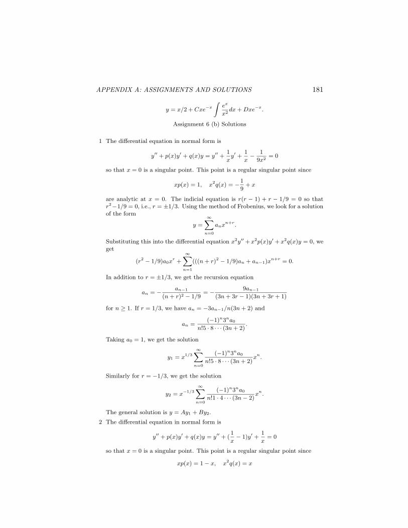
APPENDIX A: ASSIGNMENTS AND SOLUTIONS 181
y = x/2 + Cxe−x
∫ex
x2dx + Dxe−x.
Assignment 6 (b) Solutions
1 The differential equation in normal form is
y′′ + p(x)y′ + q(x)y = y′′ +1
xy′ +
1
x− 1
9x2= 0
so that x = 0 is a singular point. This point is a regular singular point since
xp(x) = 1, x2q(x) = −1
9+ x
are analytic at x = 0. The indicial equation is r(r − 1) + r − 1/9 = 0 so thatr2−1/9 = 0, i.e., r = ±1/3. Using the method of Frobenius, we look for a solutionof the form
y =
∞∑n=0
anxn+r.
Substituting this into the differential equation x2y′′ + x2p(x)y′ + x2q(x)y = 0, weget
(r2 − 1/9)a0xr +
∞∑n=1
(((n + r)2 − 1/9)an + an−1)xn+r = 0.
In addition to r = ±1/3, we get the recursion equation
an = − an−1
(n + r)2 − 1/9= − 9an−1
(3n + 3r − 1)(3n + 3r + 1)
for n ≥ 1. If r = 1/3, we have an = −3an−1/n(3n + 2) and
an =(−1)n3na0
n!5 · 8 · · · (3n + 2).
Taking a0 = 1, we get the solution
y1 = x1/3
∞∑n=0
(−1)n3na0
n!5 · 8 · · · (3n + 2)xn.
Similarly for r = −1/3, we get the solution
y2 = x−1/3
∞∑n=0
(−1)n3na0
n!1 · 4 · · · (3n− 2)xn.
The general solution is y = Ay1 + By2.
2 The differential equation in normal form is
y′′ + p(x)y′ + q(x)y = y′′ + (1
x− 1)y′ +
1
x= 0
so that x = 0 is a singular point. This point is a regular singular point since
xp(x) = 1− x, x2q(x) = x
182 ORDINARY DIFFERENTIAL EQUATIONS AND LINEAR ALGEBRA
are analytic at x = 0. The indicial equation is r(r − 1) + r = 0 so that r2 = 0,i.e., r = 0. Using the method of Frobenius, we look for a solution of the form
y =
∞∑n=0
anxn+r.
Substituting this into the differential equation x2y′′ + x2p(x)y′ + x2q(x)y = 0, weget
r2a0xr +
∞∑n=0
((n + r)2an − (n + r − 2)an−1)xn+r = 0.
This yields the recursion equation
an =n + r − 2
(n + r)2an−1, (n ≥ 1).
Hence
an(r) =(r − 1)r(r + 1) · · · (r + n− 2)
(r + 1)2(r + 2)2 · · · (r + n)2a0.
Taking r = 0, a0 = 1, we get the solution
y1 = 1− x.
To get a second solution we compute a′n(0).
a′n(r) =(r − 1)(r + 1) · · · (r + n− 2)
(r + 1)2(r + 2)2 · · · (r + n)2a0 + rbn(r).
Hence a′1(0) = 3a0. Setting r = 0, we get for n ≥ 2
a′n(0) =(−1) · 1 · 2 · · · · (n− 2)
(n!)2a0
from which an = −(n − 2)!a0/(n!)2 for n ≥ 2. Taking a0 = 1, we get as secondsolution
y2 = y1 ln(x) + 3x−∞∑
n=2
(n− 2)!
(n!)2xn.
Assignment 7(b) Solutions
1 (a) L{t sin(t)} = − dds
1s2+1
= −2s(s2+1)2
, L{t cos(t)} = − dds
ss2+1
= s2−1(s2+1)2
=1
s2+1− 2
(s2+1)2,
L{t2 sin(t)} = − d
ds
−2s
(s2 + 1)2=
6
(s2 + 1)2− 8
(s2 + 1)3, L{t2 cos(t)} = − 8s
(s2 + 1)3+
2s
(s2 + 1)2.
(b) L−1{ s(s2+1)3
} = −t2 cos(t)/8+t sin(t)/8, L−1{ 1(s2+1)3
} = 3 sin(t)/8−3t cos(t)/8−t2 sin(t)/8.
2 If Y (s) = L{y(t)}, we have (s4 − 1)Y (s)− s3 − s2 + s + 1 = 1s2+1
. Hence
Y (s) = 1(s4−1)(s2+1)
+ ((s+1)(s2−1)
s4−1= 1
(s4−1)(s2+1)+ ((s+1)
s2+1
= 18
1s−1
− 18
1s+1
+ 34
1s2+1
− 12
1(s2+1)2
+ ss2+1
.
APPENDIX A: ASSIGNMENTS AND SOLUTIONS 183
y(t) = et/8− e−t/8 + sin(t)/2 + cos(t) + t cos(t)/4.
3 If X(s) = L{x(t)}, Y (s) = L{y(t)} we have
sX(s)− 1 = −2X(s) + 3Y (s), sY (s) + 1 = X(s)− Y (s).
Hence X(s) = (s− 2)/(s2 + 3s− 1), Y (s) = (−1− s)/(s2 + 3s− 1) and
X(s) = ( 7√
1326
+ 12) 1
s+(3+√
13)/2+ (−7
√13
26+ 1
2) 1
s−(√
13−3)/2,
Y (s) = −(√
1326
+ 12) 1
s+(3+√
13)/2+ (
√13
26− 1
2) 1
s−(√
13−3)/2,
x(t) = ( 7√
1326
+ 12)e−(3+
√13)t/2 + (−7
√13
26+ 1
2)e(
√13−3)t/2,
y(t) = −(√
1326
+ 12)e−(3+
√13)t/2 + (
√13
26− 1
2)e(
√13−3)t/2
4 We have y′′ + 3y′ + 2y = 1− 2u1(t) + (sin(t) + 1)uπ(t). If Y (s) = L{y(t)}
(s2 + 3s + 2)Y (s) =1
2− 2
e−s
s+ e−πs(
−1
s2 + 1+
1
s),
since sin(t + π) = − sin(t). Hence
Y (s) =1
s(s + 1)(s + 2)+e−s −2
s(s + 1)(s + 2)+e−πs(
−1
(s2 + 1)(s + 1)(s + 2)+
1
s(s + 1)(s + 2).
Since1
s(s + 1)(s + 2)=
1
2s− 1
s + 1+
1
2(s + 2),
1
(s2 + 1)(s + 1)(s + 2)=
1
2(s + 1)− 1
5(s + 2)+
1− 3s
10(s2 + 1),
we haveY (s) = 1
2s− 1
s+1+ 1
2(s+2)+ (−1
s+ 2
s+1− 1
s+2)e−s
+( 12s− 3
2(s+1)+ 7
10(s+2)− 1
10(s2+1)− 3s
10(s2+1))e−πs.
y(t) = 12− e−t + e−2t
2+ (−1 + 2e1−t − e2−2t)u1(t)
+( 12− 3eπ−t
2+ 7e2π−2t
10+ sin(t)
10− 3 cos(t)
10)uπ(t).
y(t) =
12− e−t + 1
2e−2t, 0 ≤ t < 1,
− 12
+ (2e− 1)e−t + ( 12− e2)e−2t, 1 ≤ t < π,
(2e− 1− 32eπ)e−t + ( 1
2− e2 + 7
10e2π)e−2t + 1
10sin(t)− 3
10cos(t), π ≤ t.
184 ORDINARY DIFFERENTIAL EQUATIONS AND LINEAR ALGEBRA
Assignment #8 B Solutions
1 Taking the determinant of (1− λ −2
3 −4− λ
)
we find the characteristic polynomial to be P (λ) = λ2+3λ+2 = (λ+1)(λ+2) = 0,so the eigenvalues are λ1 = −1 and λ2 = −2. We find ∆ = tr(A)2 − 4det(A) =9 − 8 = 1 which is > 0. This indicates the eigenvalues are real and unequal,as we have found them to be. Now we need to find v1 and v2. We get v12 =
1a12
(λ1 − a11) = 1−2
(−1− 1) = 1 and v22 = 1a12
(λ2 − a11) = 1−2
(−2− 1) = 32.
This gives two linearly independent eigenvectors
v1 =
(11
)and v2 =
(132
)
Thus the general solution for this system is x(t) = c1e−tv1 + c2e
−2tv2, where c1
and c2 are arbitrary constants.As t →∞, x(t) → 0.Below are plots with c1 = c2 = 1, for the first solution (top component of x(t)),and then the second solution (bottom component of x(t)).
2 In this case, the characteristic polynomial is det(A−λI) = P (λ) = (λ+3)(λ−2) =0, hence the eigenvalues are -3 and 2, real and unequal. From the eigenvalues, weget v12 = 1
1(−3− 1) = −4 and v22 = 1
1(2− 1) = 1. The eigenvectors are
v1 =
(1−4
)and v2 =
(11
)
From this, the general solution is x(t) = c1e−3tv1 + c2e
2tv2 where c1 and c2 arearbitrary constants.As t →∞, x(t) →∞.Below are plots with c1 = c2 = 1, for the first solution (top component of x(t)),and then the second solution (bottom component of x(t)).
3 The characteristic polynomial is P (λ) = λ2 + 9 = 0. Therefore, we get complexeigenvalues λ1 = 3i and its complex conjugate λ2 = −3i. Finding v12 = 1
2(3i− 1)
and v22 = 12(−3i− 1), we get
v1,2 = r± is =
(1
−12± 3i
2
)
The general solution is x(t) = c1e−3itv1 + c2e
3itv2 where c1 and c2 are arbitraryconstants.
4 The characteristic polynomial is P (λ) = λ2 +2λ+5 = (λ+1−2i)(λ+1+2i) = 0.The complex eigenvalues are λ1 = −1+2i and its complex conjugate λ2 = −1−2i.We get v12 = 1
−4(−1 + 2i− (−1)) = −i
2and v22 = 1
−4(−1− 2i− (−1)) = i
2. The
eigenvectors are
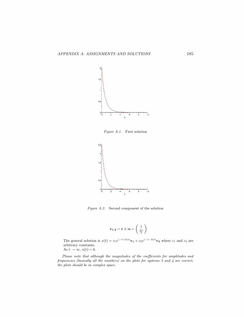
APPENDIX A: ASSIGNMENTS AND SOLUTIONS 185
Figure A.1. First solution
Figure A.2. Second component of the solution
v1,2 = r± is =
(1±i2
)
The general solution is x(t) = c1e(−1+2i)tv1 + c2e
(−1−2i)tv2 where c1 and c2 arearbitrary constants.As t →∞, x(t)→ 0.
Please note that although the magnitudes of the coefficients for amplitudes andfrequencies (basically all the numbers) on the plots for systems 3 and 4 are correct,the plots should be in complex space.
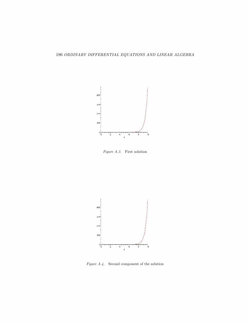
186 ORDINARY DIFFERENTIAL EQUATIONS AND LINEAR ALGEBRA
Figure A.3. First solution
Figure A.4. Second component of the solution
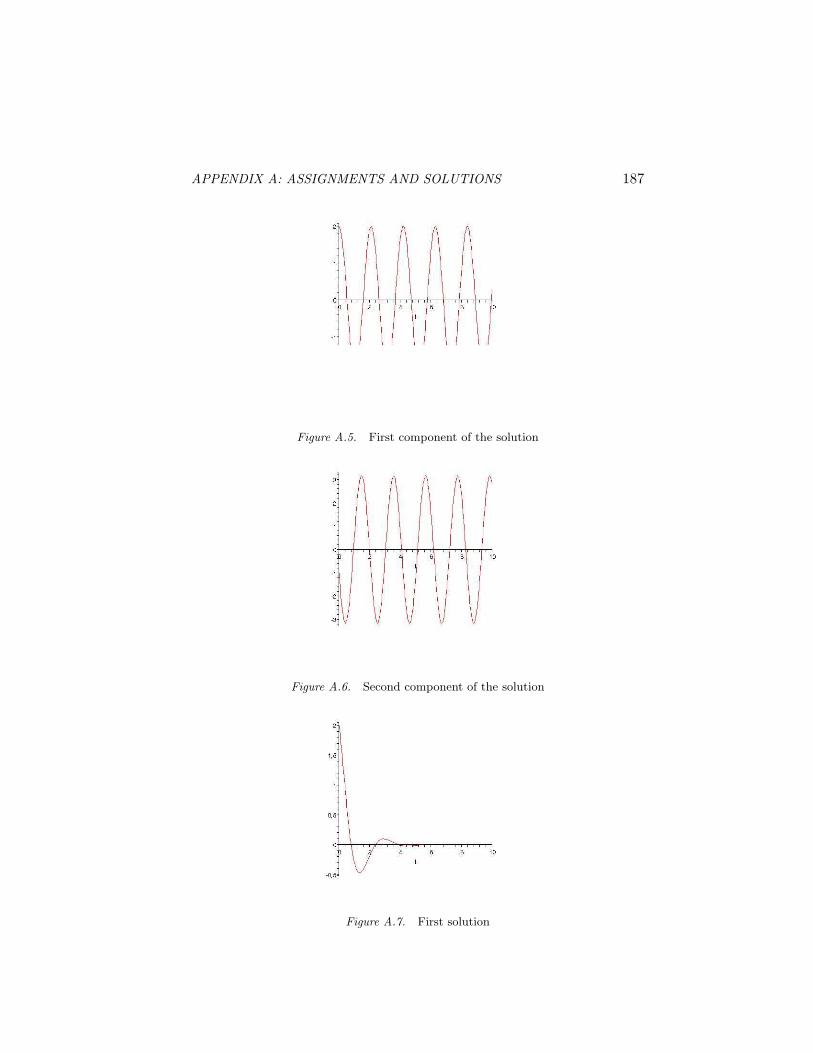
APPENDIX A: ASSIGNMENTS AND SOLUTIONS 187
Figure A.5. First component of the solution
Figure A.6. Second component of the solution
Figure A.7. First solution
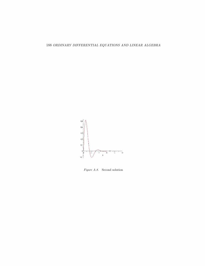
188 ORDINARY DIFFERENTIAL EQUATIONS AND LINEAR ALGEBRA
Figure A.8. Second solution
Recommended