www.studymafia.org
A
Seminar report
On
Blue Gene
Submitted in partial fulfillment of the requirement for the award of degree
Of Civil
SUBMITTED TO: SUBMITTED BY:
www.studymafia.org www.studymafia.org

www.studymafia.org
Preface
I have made this report file on the topic Blue Gene; I have tried my best to elucidate all the
relevant detail to the topic to be included in the report. While in the beginning I have tried to give
a general view about this topic.
My efforts and wholehearted co-corporation of each and everyone has ended on a successful
note. I express my sincere gratitude to …………..who assisting me throughout the preparation
of this topic. I thank him for providing me the reinforcement, confidence and most importantly
the track for the topic whenever I needed it.

www.studymafia.org
Acknowledgement
I would like to thank respected Mr…….. and Mr. ……..for giving me such a wonderful
opportunity to expand my knowledge for my own branch and giving me guidelines to present a
seminar report. It helped me a lot to realize of what we study for.
Secondly, I would like to thank my parents who patiently helped me as i went through my work
and helped to modify and eliminate some of the irrelevant or un-necessary stuffs.
Thirdly, I would like to thank my friends who helped me to make my work more organized and
well-stacked till the end.
Next, I would thank Microsoft for developing such a wonderful tool like MS Word. It helped
my work a lot to remain error-free.
Last but clearly not the least, I would thank The Almighty for giving me strength to complete
my report on time.
www.studymafia.org
Content
Introduction
The performance spectrum
Design and Analysis of the Blue Gene/L Torus Interconnection Network
Torus Network
Simulator Overview
Sample Performance Studies
Application
The protein folding problem.
Current view of folding mechanisms
References

www.studymafia.org
Introduction
The first computer in the Blue Gene series, Blue Gene/L, developed through a partnership with
Lawrence Livermore National Laboratory, cost US$100 million and is intended to scale to
speeds in the hundreds of TFLOPS, with a theoretical peak performance of 360 TFLOPS. This is
almost ten times as fast as the Earth Simulator, the fastest supercomputer in the world before
Blue Gene. In June 2004, two Blue Gene/L prototypes scored in the TOP500 Supercomputer List
at the #4 and #8 positions.
On September 29, 2004, IBM announced that a Blue Gene/L prototype at IBM Rochester
(Minnesota) had overtaken NEC's Earth Simulator as the fastest computer in the world, with a
speed of 36.01 TFLOPS, beating Earth Simulator's 35.86 TFLOPS. The machine later reached a
speed of 70.72 TFLOPS.
Linux will be the main operating system for IBM's upcoming family of "Blue Gene"
supercomputers--a major endorsement for the operating system and the open-source computing
model it represents. The decision to adopt Linux came, in part, as a result of the growing size and
strength of the open-source community. Thousands of developers around the world are
participating in the evolution of Linux. Creating a new OS inside of IBM would require a
massive engineering effort.
On March 24, 2005, the US Department of Energy announced that Blue Gene/L broke its current
world speed record, reaching 135.5 TFLOPS. This feat was possible because of doubling the
number of racks to 32 with each rack holding 1,024 compute nodes. This is still only half of the
final configuration with 65,536 compute nodes. The final Blue Gene/L installation will have a
total of 65,536 compute nodes (i.e., 216 nodes) and an additional 1024 I/O nodes. Each compute
or IO node is a single ASIC with associated DRAM memory chips. The ASIC integrates two
PowerPC 440 embedded processors, a cache sub-system and communication sub-systems. Each
node is attached to three parallel communications networks: a 3D toroidal network for peer-to-
peer communication between compute nodes, a collective network for collective communication,
and a global interrupt network for fast barriers. The I/O nodes, which run the Linux operating

www.studymafia.org
system, provide communication with the world via an Ethernet network. Finally, a separate and
private Ethernet network provides access to any node for configuration, booting and diagnostics.
Blue Gene/L compute nodes use on a minimal operating system supporting a single process
thread, and lacking interrupts and virtual memory. To allow multiple programs to run
concurrently, compute nodes can be partitioned into electronically isolated sets of nodes. The
number of nodes in a partition must be a positive integer power of 2, and must contain at least 25
= 32 nodes. The maximum partition is all nodes in the computer. To run a program on Blue
Gene/L, a partition of the computer must first be reserved. The program is then run on all the
nodes within the partition, and no other program may access nodes within the partition while it is
in use. Upon completion, the partition nodes are released for future programs to use.
With so many nodes, components will be failing frequently. Thus, the system will be able to
electrically isolate faulty hardware to allow the machine to continue to run.
In public relations terms, it is being positioned as the successor of IBM's Deep Blue chess
computer; however it bears little architectural resemblance to Deep Blue.
www.studymafia.org
Applications
Veselin Topalov, the challenger to the World Chess Champion title in 2010, confirmed in
an interview that he had used a Blue Gene/P supercomputer during his preparation for the
match.
The Blue Gene/P computer has been used to simulate approximately one percent of a
human cerebral cortex, containing 1.6 billion neurons with approximately 9 trillion
connections.
The IBM Kittyhawk project team has ported Linux to the compute nodes and
demonstrated generic Web 2.0 workloads running at scale on a Blue Gene/P. Their paper,
published in the ACM Operating Systems Review, describes a kernel driver that tunnels
Ethernet over the tree network, which results in all-to-all TCP/IP connectivity. Running
standard Linux software like MySQL, their performance results on SpecJBB rank among
the highest on record
In 2011, a Rutgers University / IBM / University of Texas team linked the KAUST Shah
een installation together with a Blue Gene/P installation at the IBM Watson Research
Center into a "federated high performance computing cloud", winning the IEEE SCALE
2011 challenge with an oil reservoir optimization application
www.studymafia.org
Technical Details
The performance spectrum
In computing, FLOPS is an abbreviation of FLoating point Operations Per Second. This is used
as a measure of a computer's performance, especially in fields of scientific calculations that make
heavy use of floating point calculations. (Note: a hertz is a cycle (or operation) per second.
Compare to MIPS -- million instructions per second.) One should speak in the singular of a
FLOPS and not of a FLOP, although the latter is frequently encountered. The final S stands for
second and does not indicate a plural. Computing devices exhibit an enormous range of
performance levels in floating-point applications, so it makes sense to introduce larger units than
the FLOPS. The standard SI prefixes can be used for this purpose, resulting in such units as the
megaFLOPS (MFLOPS, 106 FLOPS), the gigaFLOPS (GFLOPS, 109 FLOPS), the teraFLOPS
(TFLOPS, 1012 FLOPS), and the petaFLOPS (PFLOPS, 1015 FLOPS).
A cheap but modern desktop computer using, for example, a Pentium 4 or Athlon 64 CPU,
typically runs at a clock frequency in excess of 2 GHz and provides computational performance
in the range of a few GFLOPS. Even some video game consoles of the late 1990s' vintage, such
as the Gamecube and Dreamcast had performance in excess of one GFLOPS .
The original supercomputer, the Cray-1, was set up at Los Alamos National Laboratory in 1976.
The Cray-1 was capable of 80 MFLOPS (or, according to another source, 138–250 MFLOPS). In
fewer than 30 years since then, the computational speed of supercomputers has jumped a
millionfold.
The fastest computer in the world as of November 5, 2004, the IBM Blue Gene supercomputer,
measures 70.72 TFLOPS. This supercomputer was a prototype of the Blue Gene/L machine IBM
is building for the Lawrence Livermore National Laboratory in California. During a speed test on
24 March 2005, it was rated at 135.5 TFLOPS. Blue Gene's new record was achieved by
doubling the number of current racks to 32. Each rack holds 1,024 processors, yet the chips are

www.studymafia.org
the same as those found in high-end computers. The complete version will have a total of 64
racks and a theoretical speed measured at 360 TFLOPS.

www.studymafia.org
Major features
The Blue Gene/L supercomputer was unique in the following aspects:
Trading the speed of processors for lower power consumption. Blue Gene/L used low
frequency and low power embedded PowerPC cores with floating point accelerators.
While the performance of each chip was relatively low, the system could achieve better
performance to energy ratio, for applications that could use larger numbers of nodes.
Dual processors per node with two working modes: co-processor mode where one
processor handles computation and the other handles communication; and virtual-node
mode, where both processors are available to run user code, but the processors share both
the computation and the communication load.
System-on-a-chip design. All node components were embedded on one chip, with the
exception of 512 MB external DRAM.
A large number of nodes (scalable in increments of 1024 up to at least 65,536)
Three-dimensional torus interconnect with auxiliary networks for global communications
(broadcast and reductions), I/O, and management
Lightweight OS per node for minimum system overhead (system noise).

www.studymafia.org
Architecture Details
Blue Gene/L (BG/L) is a scientific and engineering, message-passing, supercomputer that IBM is
developing with partial funding from the U.S. Department of Energy Lawrence Livermore
National Laboratory. A 64K node system is scheduled to be delivered to Livermore, while a 20K
node system will be installed at the IBM T.J. Watson Research Center for use in life sciences
computing, primarily protein folding.
BG/L is built using system-on-a-chip technology in which all functions of a node (except for
main memory) are integrated onto a single ASIC. This ASIC includes two 32- bit Power PC
cores (the 440); the 440 was developed for embedded applications. Associated with each core is
a 64- bit “double” floating-point unit (FPU) that can operate in SIMD mode. Each (single) FPU
can execute up to two multiply-adds per cycle, meaning that the peak performance of the chip is
8 floating-point operations per cycle. Each 440 has its own instruction and data caches (each
32KB), a small L2 cache that primarily serves as a pre-fetch buffer, a 4MB shared L3 cache built
from embedded DRAM, and a DDR memory controller. In addition, the logic for five different
networks is integrated onto the ASIC. These networks include a JTAG control and monitoring
network, a Gbit Ethernet macro, a global barrier and alert network, a “tree” network for
broadcasts and combining operations such as those used in the MPI collective communications
library, and a three dimensional torus network for point-point communications between nodes.
The ASIC can be used as either an I/O node or as a Compute node. I/O nodes have their Ethernet
macro connected to an external switch enabling connectivity to hosts, however they do not use
the torus network. Compute nodes do not connect their Ethernet, and talk to the I/O nodes over
the tree network. The Livermore machine will have 64 Compute nodes for each I/O node. I/O
nodes will have at least 512MB and Compute nodes will have at least 256 MB of memory,
depending on the cost of memory at the time of delivery. Because of the high level of integration
and relatively low target clock speed (700 MHz target), the system is designed to deliver
unprecedented aggregate performance at both low cost and low power consumption. At this
clock rate, each node has a peak of 5.6 GFlops, while the 64K node system has a peak of 367
Tera Flops. Each ASIC will consume only 12 watts of power. Because of the low power, a very
high density of packaging can be achieved.Two compute ASICs and their associated memory are
www.studymafia.org
packaged onto a compute card, 16 compute cards are mounted on a node card, and 16 node cards
are packaged in a 512 node midplane. Two midplanes are packaged in a 1024 node rack, which
is about the size of a large refrigerator. Because the 440 core does not contain shared memory
support, the L1 caches of the two cores on the same ASIC are not coherent. Memory is
consistent from the L2 on out, but software is required to appropriately manage the L1’s. The
system can operate in one of two modes. In communications coprocessor mode, one core is
responsible for computing while the other core handles most messaging functions. Careful
software coordination is required in this mode to overcome the lack of L1 coherence. When
configured in this mode, the peak performance of the 64K node system is 183 Tera Flops. In the
second mode, “virtual node” mode, each core has its own memory space and each core is
responsible for both computing and message handling; the system has two sets of network
injection and reception FIFOs, so that both cores can simultaneously access the network
interfaces.
www.studymafia.org
Design and Analysis of the Blue Gene/L Torus Interconnection
Network
Torus Network
Many of the design decisions were driven by simulation performance studies. The torus network
uses dynamic routing with virtual cut through buffering. A torus was chosen because it provides
high bandwidth nearest neighbor connectivity, which is common in scientific applications, but
also for its scalability, cost and packaging considerations. A torus requires no long cables and,
because the network is integrated onto the same chip that does computing, no separate switch is
required. Previous supercomputers such as the Cray T3E have also used torus networks. Torus
packets are variable in size – from 32 to 256 bytes in increments of 32 byte chunks. The first
eight bytes of each packet contain link level protocol information (e.g., sequence number) and
routing information including destination, virtual channel and size. A 24-bit CRC is appended to
each packet, along with a one byte valid indicator. The CRC permits link level checking of each
packet received, and a timeout mechanism is used for retransmission of corrupted packets. The
error detection and recovery protocol is similar to that used in IBM SP interconnection networks
as well as in the HIPPI standard. For routing, the header includes six “hint” bits, which indicate
in which directions the packet may be routed. For example, hint bits of 100100 means that the
packet can be routed in the x+ and y- directions. Either the x+ or x- hint bits, but not both, may
be set. If no x hops are required, the x hint bits are set to 0. Each node maintains registers that
contain the coordinates of its neighbors, and hint bits are set to 0 when a packet leaves a node in
a direction such that it will arrive at its destination in that dimension. These hint bits appear early
in the header, so that arbitration may be efficiently pipelined. The hint bits can be initialized
either by software or hardware; if done by hardware, a set of two registers per dimension is used
to determine the appropriate directions. These registers can be configured to provide minimal
hop routing. The routing is accomplished entirely by examining the hint bits and virtual
channels, i.e., there are no routing tables. Packets may be either dynamically or statically (xyz)
routed. Besides point-topoint packets, a bit in the header may be set that causes a packet to be
broadcast down any dimension. The hardware does not have the capability to route around
“dead” nodes or links, however, software can set the hint bits appropriately so that such nodes
www.studymafia.org
are avoided; full connectivity can be maintained when there are up to three faulty nodes,
provided they are not co-linear.
The torus logic consists of three major units, a processor interface, a send unit and a receive unit.
The processor interface consists of network injection and reception FIFOs. Access to these
FIFOs is via the double FPU registers, i.e., data is loaded into the FIFOs via 128 bit memory
mapped stores from a pair of FPU registers, and data is read from the FIFOs via 128 bit loads to
the FPU registers. There are a total of 8 injection FIFOs organized into two groups: two high
priority (for inter-node OS messages) and six normal priority FIFOs, which are sufficient for
nearest neighbor connectivity. Packets in all FIFOs can go out in any direction. Each group of
reception FIFOs contains 7 FIFOs, one high priority and one dedicated to each of the incoming
directions. More specifically, there is a dedicated bus between each receiver and its
corresponding reception FIFO. Up to six injection and six reception FIFOs may be
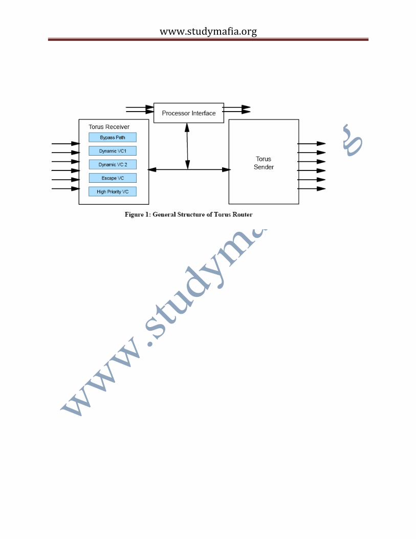
simultaneously active. Each of the six receivers, as shown in Figure 1, has four virtual channels
(VCs). Multiple VCs help reduce head-ofline blocking [4], but in addition, mesh networks
including tori with dynamic routing, can deadlock unless appropriate additional “escape” VCs
are provided. We use a recent, elegant solution to this problem, the “bubble” escape VC as
proposed in BG/L has two dynamic VCs, one bubble escape VC that can be used both for
deadlock prevention and static routing, and one high priority bubble VC. Each VC has 1 KB of
buffering, enough for four full-sized packets. In addition to the VCs, the receivers include a
“bypass” channel so that packets can flow through a node without entering the VC buffers, under
appropriate circumstances. Dynamic packets can only enter the bubble escape VC if no valid
dynamic VCs are available. A token flow control algorithm is used to prevent overflowing the
VC buffers. Each token represents a 32B chunk. For simplicity in the arbiters, a VC is marked as
unavailable unless 8 tokens (a full-sized packet) are available. However, token counts for packets
on dynamic VCs are incremented and decremented according to the size of the packet. The
bubble rules, as outlined in require that tokens for one full-sized packet are required for a packet
already on the bubble VC to advance, but that tokens for two full-sized packets are required for a
packet to enter the bubble VC, upon either injection, a turn into a new direction, or when a
dynamic VC packet enters the bubble. This rule ensures that buffer space for one packet is
always available after an insertion and thus some packet can always, eventually move. However,
www.studymafia.org
we discovered that this rule is incomplete for variable-sized packets when our simulator
deadlocked using this rule. With this rule, the remaining free space for one full-sized packet can
become fragmented resulting in a potential deadlock. To prevent this, the bubble rules are simply
modified so that each packet on the bubble is accounted for as if it were a fullsized (8 chunk)
packet. Eight byte acknowledgement (ack-only) or combined token-acknowledgement (token-
ack) packets are returned when packets are either successfully received, or when space has freed
up in a VC. Acknowledgements permit the torus send units to delete packets from their
retransmission FIFOs, which are used in the error recovery protocol. The send units also arbitrate
between requests from the receiver and injection units. Due to the density of packaging and pin
constraints, each link is bit serial. The torus is internally clocked at onefourth the rate of the
processor, so at the target 700 MHz clock rate, each torus link is 175 MB/sec. There are
sufficient internal busses so that each of the 6 outgoing and 6 incoming links can be
simultaneously busy; thus each node can be sending and receiving 1.05 GB/sec. In addition,
there are two transfer busses (paths) coming out of each receiver that connect with the senders.
Thus, a single receiver can have up to 4 simultaneous transfers, e.g., one to its normal reception
FIFO, one to the high priority reception FIFO, and two to two different senders.
Arbitration is distributed and pipelined, but occurs in three basic phases. It generalizes an
approach used in [3] and represents tradeoffs between complexity, performance, and ability to
meet timing constraints. First, each packet at the head of the injection or VC FIFOs decides in
which direction and on what VC it prefers to move. For statically routed packets, there is only
one valid choice, but dynamically routed packets may have many choices. The preferred
direction and VC are selected using a modified “Join the Shortest Queue” (JSQ) algorithm as
follows. The senders provide the receivers and injection FIFOs with a bit indicating both link and
token availability for each VC in each direction. This bit vector is and-ed with a bit vector of
possible moves constructed from the packet’s hint bits and VC. This defines the set of possible
and available arbitration requests. In addition, the sender provides 2 bits for each VC indicting
one of four ranges of available downstream tokens. Of all the possible and available dynamic
direction/VC pairs, the packet selects the one with the most available downstream tokens. Ties
are randomly broken. If no dynamic direction/VC combination is available, the packet will
request its bubble escape direction/VC pair (if available), and if that is also unavailable, the
www.studymafia.org
packet makes no arbitration request. This is a somewhat simplified description since bus
availability must also be taken into account. In addition, when a packet reaches its destination,
the “direction” requested is simply the corresponding reception FIFO. Second, since each
receiver has multiple VC FIFOs (plus the bypass) an arbitration phase is required to determine
which of the requesting packets in the receiver wins the right to request. If a high priority packet
is requesting, it wins. Barring that, a modified “Serve the Longest Queue” (SLQ) is used, based
on 2 bit (4 ranges) FIFO Fullness indicators, i.e., the packet from the most full VC (as measured
to within the 2 bits of granularity) wins. However, this cannot always be used since doing so may
completely block out a VC. Therefore, a certain (programmable) fraction of the arbitration cycles
are designated SLQ cycles in which the above algorithm is used, while the remaining cycles
select the winner
randomly. A packet on the bypass channel always receives the lowest priority (unless it is a high
priority packet). Third, the receivers and injection FIFOs present their requests to the senders.
Note that on a given cycle a receiver will present at most one request to the senders. Thus each
sender arbiter can operate independently. The sender gives highest priority to token-ack or ack-
only packets, if any. Barring that, the senders tend to favor packets already in the network and
use a similar modified SLQ algorithm in which there are SLQ cycles and random cycles. In
particular, a certain programmable fraction of cycles (typically 1.0) give priority to packets
already in the network (unless the only high priority packet requesting is in an injection FIFO).
On such cycles the modified SLQ algorithm is used. Higher priority can be given to injection
packets by lowering above in-network priority fraction. On cycles in which injection packets
receive priority (barring in-network high priority packets), the modified SLQ algorithm is also
used.

www.studymafia.org
Simulator Overview
Given the complexity and scale of the BG/L interconnection network, having an accurate
performance simulator was essential during the design phase of the project. Due to the potential
size of such a model, simulation speed was a significant concern and a proven shared memory
parallel simulation approach was selected. In particular, parallel simulation on shared memory
machines has been shown to be very effective in simulating interconnection networks whereas
success with message passing parallel interconnection network simulators is harder to come by
.We also recognized the difficulties in developing an execution driven simulator for a system
with up to 64K processes, and therefore decided upon a simulator that would primarily be driven
by application pseudo-codes, in which message passing calls could be easily passed to the
simulator; such calls include the time since the last call (the execution burst time), the destination
and size of the message, etc. This pseudo-code included a subset of the MPI point to point
messaging calls as a workload driver for the simulator. We also extended the IBM UTE trace
capture utility that runs on IBM SP machines and were able to use such traces as simulator inputs
(for up to several hundreds of nodes). The basic unit of simulation time is a network cycle, which
is defined to be the time it takes to transfer one byte. As BG/L is organized around 512 node
(8x8x8) midplanes, the simulator partitions its work on a midplane basis, i.e., all nodes on the
same midplane are simulated by the same processor (thread) and midplanes are assigned to
threads in as even a manner as possible.
Because different threads are concurrently executing, the local simulation clocks of the threads
need to be properly synchronized. To deal with this problem, we use a simple but effective
“conservative” parallel simulation protocol known as “YAWNS” .In particular, we take
advantage of the fact that the minimum transit time between midplanes is known and is at least
some constant w≥1 cycles. In this protocol, time “windows” of length w are simulated in parallel
by each of the threads. Consider an event that is executed during the window (starting at time t)
on processor i that is destined to arrive on processor j in the future; such an event represents the
arrival of the first byte of a packet. Since the minimum transit time is w, the arrival cannot occur
during the current window, represented by the interval [t, t+w-1]. Processor i simply puts a
pointer to the event on an i-to-j linked list. When each processor reaches the end of the window,
www.studymafia.org
it enters a barrier synchronization. Upon leaving the barrier, each processor is sure that every
other processor has executed all events up to time t+w-1 and that all inter-processor events are on
the appropriate inter-processor linked lists. Processor j can therefore go through all its i-to-j
linked lists, remove events from them, and put the events on its own future event list. Once this
is done, the processors can simulate the next window [t+w, t+2w-1]. If w=1, then this protocol
requires a barrier synchronization every cycle, however, on BG/L, the minimum inter-midplane
delay will be approximately w=10 network cycles. When a large number of BG/L nodes are
being simulated, each processor will execute many events during a window, i.e., between
barriers, and thus the simulator should obtain good speedups. The simulator runs on a 16-way
IBM “nighthawk” SMP with 64 GB of memory. The model of the torus hardware contains close
to 100 resources per node (links, VC token counters, busses, FIFOs, etc), so that a full 64K node
system can be thought of as a large queuing network with approximately 6 million resources. It
consumes a large amount of memory and runs slowly; a 32K node simulation of fully loaded
network advances at about 0.25 microseconds of BG/L time per second of wall clock time.
However, it obtains excellent speedup, typically more than 12 on 16 nodes, and sometimes
achieves superlinear speedup due to the private 8MB L3 caches on the SMP and the smaller per
node memory footprint of the parallel simulator. The model, which was written before the
VHDL, is thought to be a quite accurate representation of the BG/L hardware, although a number
of simplifications were made. For example, in BG/L the arbitration is pipelined and occurs over
several cycles. In the simulator, this is modeled as a delay of several cycles followed by
presentation of the arbitration request. Because the simulator focuses on what happens once
packets are inside the network, a gross simplification was the assumption that the injection
FIFOs were of infinite size, and that packets are placed in these FIFOs as early as possible rather
than as space frees up in the FIFOs. This has little effect on network response time and
throughput measurements during the middle of a run, but can affect the dynamics particularly
near the end of runs. The simulator also did not model the error recovery protocol, i.e., no link
errors were simulated and the ackonly packets that are occasionally sent if a link is idle for a long
time were not modeled. However, the arbitration algorithms and token flow control are modeled
to a high level of detail.
www.studymafia.org
Sample Performance Studies
In this section, we present some examples of use of the simulator to study design trade-offs in
BG/L. The studies presented are illustrative and sometimes use assumptions and corresponding
parameters about the system that do not reflect the final BG/L design.
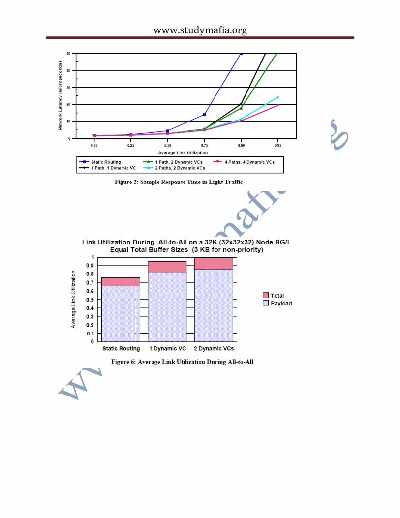
Response Time in Light Traffic: Figure 2 plots the response time for various 32K node BG/L
configurations when the workload driver generates packets for random destinations and the
packet generation rate is low enough so that the average link utilization is less than one. This
Figure compares static routing to dynamic routing with one or more dynamic VCs and one or
more busses (paths) connecting receivers to senders. Simpler, random, arbitration rules than SLQ
and JSQ were used and the plot was generated early in our studies when the target link
bandwidth was 350 MB/sec. (The 350 MB/sec. assumption essentially only affects results by a
rescaling of the y-axis.) The figure shows the clear benefit of dynamic over static routing. It also
shows that there is little benefit in increasing the number of dynamic VCs unless the number of
paths is also increased. Finally, it shows only marginal benefit in going from a 2 VC/2 path to 4
VC/4 path configuration.
All-to-All: MPI_AlltoAll is an important MPI collective communications operation in which
every node sends a different message to every other node. plots the average link utilization
during the communications pattern implied by this collective. The Figure again shows the benefit
of dynamic over static routing. For this pattern, there is marginal benefit in going from 1 to 2
dynamic VCs, but what is important is that the average link utilization is, at approximately 98%,
close to the theoretical peak. This peak includes the overhead for the token-ack packets, the
packet headers and the 4 byte CRC trailers. A reasonable assumption for the BG/L software is
that each packet carries 240 bytes of payload, and with this assumption the plot shows that the
payload occupies 87% of the links. Not shown in these plots is the fact that a very low
percentage of the traffic flows on the escape bubble VC and that statistics collected during the
run showed that few of the VC buffers are full. Three-dimensional FFT algorithms often require
the equivalent of an All-to-All, but on a subset of the nodes consisting of either a plane or a line
www.studymafia.org
in the torus. Simulations of these communications patterns also resulted in near-peak
performance. The above simulation was for a symmetric BG/L. However, the situation is not so
optimistic for an asymmetric BG/L. For example, the 64K node system will be a 64x32x32 node
torus. In such a system, the average number of hops in the x dimension is twice that of the y and
z dimensions, so that even if every x link is 100% busy, the y and z links can be at most 50%
busy. Thus, the peak link utilization is at most 66.7%. Since 12% of that is overhead, the best
possible payload utilization is 59%. However, we expect significantly more blocking and
throughput degradation due to full VC buffers. Indeed a simulation of the All-to-All
communications pattern on a 32x16x16 torus resulted in an average link utilization of 49% and
payload utilization of 44%, corresponding to 74% of the peak. This figure is probably somewhat
pessimistic due to the simulator artifact of infinite-sized injection FIFOs, which distorts the
effects at the end of the simulation. We also believe that appropriate injection flow control
software algorithms can reduce VC buffer blocking and achieve closer to peak performance.
Nevertheless, the above study points out a disadvantage of the torus architecture for asymmetric
machines in which the application cannot be easily mapped so as to result in a close proximity
communications pattern.
Virtual Channel Architecture: Here we consider several different deadlock prevention escape VC
architectures. The first proposed has two escape VCs per direction. Each dimension has a
“dateline.” Before crossing the dateline, the escape VC is the lower numbered of the pair, but
after crossing the dateline the escape VC is the higher numbered of the pair. In addition we
consider dimension ordered or direction ordered escape VCs. In dimension ordered, the escape
VC is x first, then y if no x hops remain, then z if no x or y hops remain. In direction ordered, the
escape VCs are ordered by x+, y+, z+, x-, y-, z- (other orderings are possible). We also consider
dimension and direction ordered escape VCs for the bubble escape. We again use the hot region
workload where the hot region starts at coordinates (0,0,0) and the datelines are set at the
maximum coordinate value in each dimension. plots the throughput as a function of time. The
dimension ordered dateline pair shows particularly poor and wild behavior, with a steep decline
in throughput, followed by a rise and then another steep decline. plots the throughput on a per
VC basis for a longer period of time. The decreasing and increasing bandwidth waves persist
even over this much longer time scale. An appreciable fraction of the traffic flows on the escape

www.studymafia.org
VCs, indicating a high level of VC buffer occupation. What causes these waves? First, the
placement of the dateline causes an asymmetry in the torus, whereas the bubble escape is
perfectly symmetrical in each dimension. Since there are two escape VCs, we thought it likely
that packets at the head of the VC buffers could be waiting for one of the escape VCs but tokens
are returned for the other escape VC. In such a situation, no packets could move even though the
link may be available and downstream buffer space is available. To confirm this, the simulator
was instrumented to collect additional statistics. In particular, we measured the fraction of time a
token-ack is returned that frees at least one previously blocked packet to move. plots this
unblocking probability along with the throughput as a function of time. The unblocking
probability is relatively constant for the bubble (after the initial decline), but varies directly with
the throughput for the dateline pair; when the unblocking probability increases, the throughput
increases and vice-versa.
Performance Verification: To verify the VHDL logic of the torus, we built a multi-node
verification testbench. This testbench, which runs on the Cadence VHDL simulator, consisted of
workload drivers that inject packets into the injection FIFOs, links between nodes on which bits
could be corrupted to test the error recovery protocol, and packet checkers that pull packets out
of the reception FIFOs and check them for a variety of conditions, such as whether the packet
arrived at the correct destination and whether its contents were received correctly. The workload
drivers could be flexibly configured to simulate a number of different traffic patterns. As we
neared the end of the logic verification process, we wanted to ensure that network performance
was as intended. One of the benchmarks we tested was the All-to- All. The VHDL simulator was
limited (by memory) to a maximum of 64 nodes, so we simulated both a 4x4x4 torus and an
8x8x1 torus and compared the average link utilizations to those predicted by the performance
simulator. While these agreed to within 2%, the VHDL (corresponding to the actual network
hardware) indicated that VC buffers were fuller than that predicted by the performance
simulator. A close inspection of the arbitration logic revealed that a one cycle gap in the
arbitration pipeline of the receivers could occur when all possible outgoing links/VCs were busy.
This gap was sufficient to permit packets from the injection FIFOs to sneak into the network,
leading to fuller VCs than intended. A simple fix to eliminate this possibility was implemented,
and subsequent VHDL simulations indicated greatly reduced levels of VC buffer occupation.
www.studymafia.org
www.studymafia.org
www.studymafia.org
Application
Machines like Blue Gene/L are designed to handle data-intensive applications like content
distribution, simulations, and modeling, webserving, data mining or business intelligence.
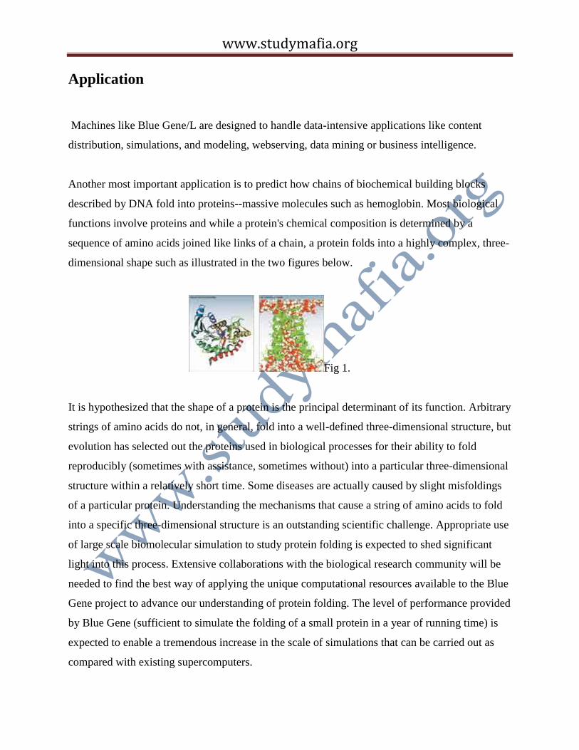
Another most important application is to predict how chains of biochemical building blocks
described by DNA fold into proteins--massive molecules such as hemoglobin. Most biological
functions involve proteins and while a protein's chemical composition is determined by a
sequence of amino acids joined like links of a chain, a protein folds into a highly complex, three-
dimensional shape such as illustrated in the two figures below.
Fig 1.
It is hypothesized that the shape of a protein is the principal determinant of its function. Arbitrary
strings of amino acids do not, in general, fold into a well-defined three-dimensional structure, but
evolution has selected out the proteins used in biological processes for their ability to fold
reproducibly (sometimes with assistance, sometimes without) into a particular three-dimensional
structure within a relatively short time. Some diseases are actually caused by slight misfoldings
of a particular protein. Understanding the mechanisms that cause a string of amino acids to fold
into a specific three-dimensional structure is an outstanding scientific challenge. Appropriate use
of large scale biomolecular simulation to study protein folding is expected to shed significant
light into this process. Extensive collaborations with the biological research community will be
needed to find the best way of applying the unique computational resources available to the Blue
Gene project to advance our understanding of protein folding. The level of performance provided
by Blue Gene (sufficient to simulate the folding of a small protein in a year of running time) is
expected to enable a tremendous increase in the scale of simulations that can be carried out as
compared with existing supercomputers.

www.studymafia.org
The scientific community considers protein folding one of the most significant "grand
challenges" -- a fundamental problem in science or engineering that has broad economic and
scientific impact and whose solution can be advanced only by applying high-performance
computing technologies.
Proteins control all cellular processes in the human body. Comprising strings of amino acids that
are joined like links of a chain, a protein folds into a highly complex, three-dimensional shape
that determines its function. Any change in shape
dramatically alters the function of a protein, and even the slightest change in the folding process
can turn a desirable protein into a disease.
Better understanding of how proteins fold will give scientists and doctors better insight into
diseases and ways to combat them. Pharmaceutical companies could design high-tech
prescription drugs customized to the specific needs of individual people. And doctors could
respond more rapidly to changes in bacteria and viruses that cause them to become drug-
resistant.
The human genome is currently thought to contain approximately 40000 genes, which code for a
much larger number of proteins through alternative splicing and post-translational modification,
a molecular toolkit assembled to handle a huge diversity of functions. An understanding of how
proteins function is essential for understanding the cell life cycle and metabolism, how cells send
signals to their environment, and how cells receive and process signals from their environment.
An understanding of protein structure and function can serve as a basis for innovation in new
therapies, diagnostic devices, and even industrial applications. When proteins fold into the
wrong structure, the results can be fatal, e.g., “mad cow” disease probably results from an
autocatalyzed wrong fold in the prion protein6 and cystic fibrosis is also connected with protein
(mis)folding.
Protein architecture. Protein architecture8 is based on three principles:
The formation of a polymer chain .
www.studymafia.org
The folding of this chain into a compact function-enabling structure, or native structure .
Post-translational modification of the folded structure .
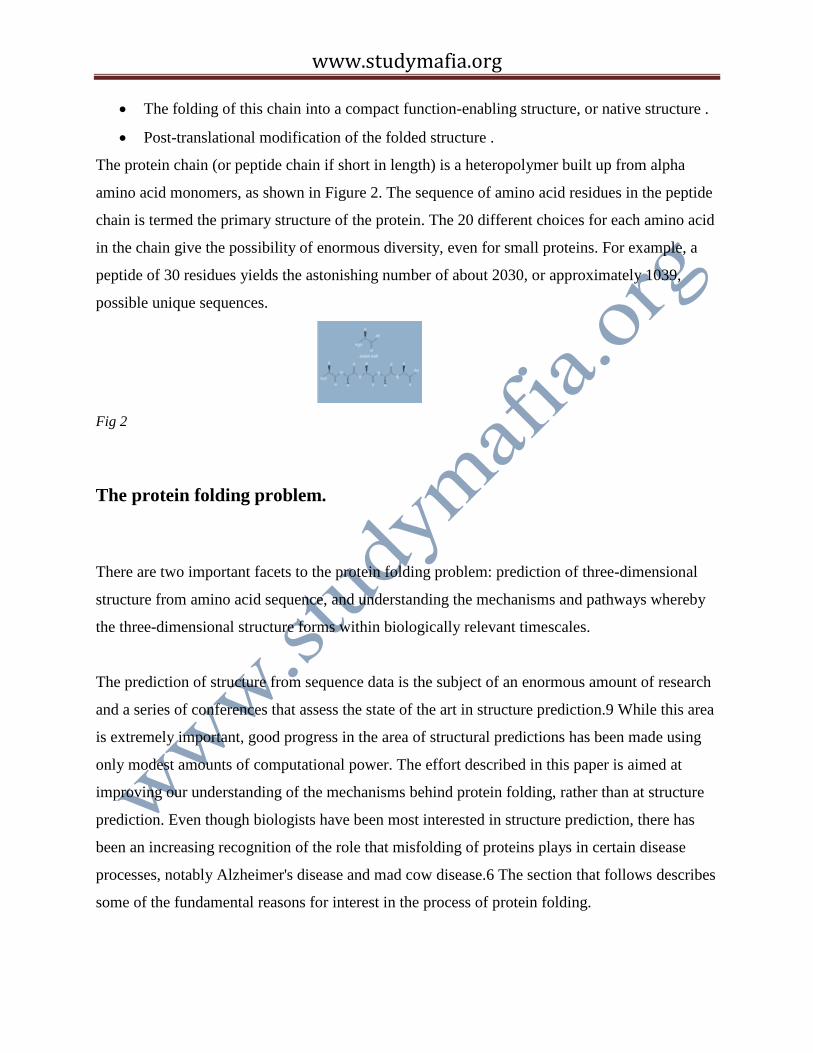
The protein chain (or peptide chain if short in length) is a heteropolymer built up from alpha
amino acid monomers, as shown in Figure 2. The sequence of amino acid residues in the peptide
chain is termed the primary structure of the protein. The 20 different choices for each amino acid
in the chain give the possibility of enormous diversity, even for small proteins. For example, a
peptide of 30 residues yields the astonishing number of about 2030, or approximately 1039,
possible unique sequences.
Fig 2
The protein folding problem.
There are two important facets to the protein folding problem: prediction of three-dimensional
structure from amino acid sequence, and understanding the mechanisms and pathways whereby
the three-dimensional structure forms within biologically relevant timescales.
The prediction of structure from sequence data is the subject of an enormous amount of research
and a series of conferences that assess the state of the art in structure prediction.9 While this area
is extremely important, good progress in the area of structural predictions has been made using
only modest amounts of computational power. The effort described in this paper is aimed at
improving our understanding of the mechanisms behind protein folding, rather than at structure
prediction. Even though biologists have been most interested in structure prediction, there has
been an increasing recognition of the role that misfolding of proteins plays in certain disease
processes, notably Alzheimer's disease and mad cow disease.6 The section that follows describes
some of the fundamental reasons for interest in the process of protein folding.
www.studymafia.org
Current view of folding mechanisms.
A simplistic but illustrative way of viewing protein folding is to note that the amino acid R
groups (see Figure 2, caption) fall into three main classes: (1) charged, (2) hydrophilic (“water-
loving”), and (3) hydrophobic (“water-hating”). In the simplest picture, the folded state of the
peptide chain is stabilized primarily (for a globular protein in water), by the sequestration of
much of the hydrophobic groups into the core of the protein—out of contact with water, while
the hydrophilic and charged groups remain in contact with water. The stability can be described
in terms of the Gibbs free-energy change G
G = H – TS,
where H is the enthalpy change and S is the entropy change. H is negative due to the more
favorable hydrophobic interactions in the folded state, but so is S because the folded state is
much more ordered and has lower entropy than the unfolded state. The balance between the
enthalpy and entropy terms is a delicate one, and the total free-energy change is only of order 15
kilocalories per mole. Evidently the internal hydrophobic/external hydrophilic packing
requirement places strong constraints on the amino acid sequence, as does the requirement that
the native state be kinetically accessible.
It is helpful to think of the physics of the folding process as a “free-energy funnel Since the
folding process is slow relative to motions at atomic scale, we can think of partially folded
configurations as having a quasi-equilibrium value of the free energy. The free energy surface
may be displayed as a function of some reduced dimensionality representation of the system
configuration in a given state of the protein.12 . The most unfolded configurations are the most
numerous, but have the highest free energy, and occur on the rim of the funnel. Going into the
funnel represents a loss of number of configurations (decrease of entropy), but a gradual
decrease in free energy, until the native state with very few configurations and the lowest free
energy is reached at the bottom of the funnel. The walls of the funnel contain only relatively
shallow subsidiary minima, which can trap the folding protein in non-native states, but only for a
short time. Now the evolution of the system as it folds can be described in terms of the funnel.
The system starts off in a physically probable state on the rim of the funnel, and then makes
www.studymafia.org
transitions to a series of physically accessible states within the funnel, until the bottom of the
funnel is gradually approached.
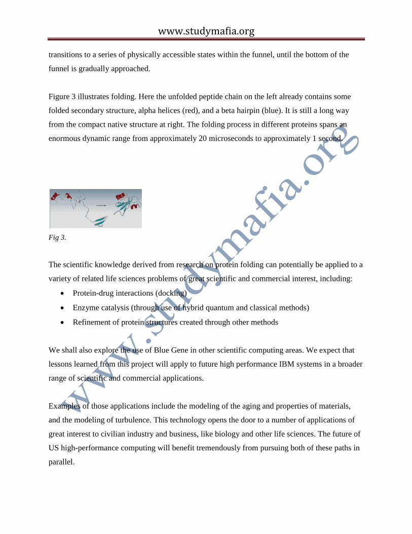
Figure 3 illustrates folding. Here the unfolded peptide chain on the left already contains some
folded secondary structure, alpha helices (red), and a beta hairpin (blue). It is still a long way
from the compact native structure at right. The folding process in different proteins spans an
enormous dynamic range from approximately 20 microseconds to approximately 1 second.
Fig 3.
The scientific knowledge derived from research on protein folding can potentially be applied to a
variety of related life sciences problems of great scientific and commercial interest, including:
Protein-drug interactions (docking)
Enzyme catalysis (through use of hybrid quantum and classical methods)
Refinement of protein structures created through other methods
We shall also explore the use of Blue Gene in other scientific computing areas. We expect that
lessons learned from this project will apply to future high performance IBM systems in a broader
range of scientific and commercial applications.
Examples of those applications include the modeling of the aging and properties of materials,
and the modeling of turbulence. This technology opens the door to a number of applications of
great interest to civilian industry and business, like biology and other life sciences. The future of
US high-performance computing will benefit tremendously from pursuing both of these paths in
parallel.

www.studymafia.org
"One day, you're going to be able to walk into a doctor's office and have a computer
analyze a tissue sample, identify the pathogen that ails you, and then instantly prescribe a
treatment best suited to your specific illness and individual genetic makeup."
Consider the following three types of protein science studies that might employ large-scale
numerical simulation techniques:
Structure prediction
Folding pathway characterization
Folding kinetics
Protein structure prediction can be carried out using a large number of techniques8 and, as
previously discussed, it is unnecessary to spend a “petaflop year” on the prediction of a single
protein structure. That said, there is some reason to believe that atomistic simulation techniques
may be useful in refining structures obtained by other methods.
Folding pathway characterization typically involves the study of thermodynamic properties of a
protein in quasi-equilibrium during the folding process. Mapping out the free-energy “landscape”
that the protein traverses as it samples conformations during the folding process can give insights
into the nature of intermediate states along the folding pathway and into the “ruggedness” of the
free-energy surface that is traversed during this process. Because such studies involve
computations of average values of selected functions of the system's state, one has the choice of
either averaging over time as the system samples a large number of states (molecular dynamics)
or averaging over configurations (Monte Carlo). Aggressive sampling techniques that may
improve the computational efficiency with which such averages can be computed can be used to
good effect in these studies. Simulation techniques to compute these averages over the
appropriate thermodynamic ensembles are available.
Simulation studies of folding kinetics are aimed at understanding the rates at which the protein
makes transitions between various conformations. In this case, the calculation of thermodynamic
averages is not enough; the actual dynamics of the system must be simulated with sufficient
accuracy to allow estimation of rates. Of course, a large number of transition events must be
simulated in order to derive rate estimates with reasonable statistical uncertainties. Another
www.studymafia.org
challenge faced in such simulations is that the simulation techniques used to reproduce
thermodynamic averages in ensembles other than constant particle number, volume, and energy
(NVE) are, strictly speaking, inappropriate for studies of folding kinetics.
Challenges for computational modeling
The current expectation is that it will be sufficient to use classical techniques, such as molecular
dynamics (MD), to model proteins in the Blue Gene project. This is because many aspects of the
protein folding process do not involve the making and breaking of covalent bonds. While
disulfide bonds play a role in many protein structures, their formation will not be addressed by
classical atomistic simulations. In classical atomistic approaches, a model for the interatomic
interactions is used. This is known as a potential, or force field, since the forces on all the
particles can be computed from it, if one has its mathematical expression and all its parameters.
The MD approach is to compute all the forces on all the atoms of the computer model of the
protein and solvent, then use that force to compute the new positions of all the atoms a very short
time later. By doing this repeatedly, a trajectory of the atoms of the system can be traced out,
producing atomic coordinates as a function of time.
system samples a large number of states (molecular dynamics) or averaging over configurations
(Monte Carlo). Aggressive sampling techniques that may improve the computational efficiency
with which such averages can be computed can be used to good effect in these studies.
Simulation techniques to compute these averages over the appropriate thermodynamic ensembles
are available.
Simulation studies of folding kinetics are aimed at understanding the rates at which the protein
makes transitions between various conformations. In this case, the calculation of thermodynamic
averages is not enough; the actual dynamics of the system must be simulated with sufficient
accuracy to allow estimation of rates. Of course, a large number of transition events must be
simulated in order to derive rate estimates with reasonable statistical uncertainties. Another

www.studymafia.org
challenge faced in such simulations is that the simulation techniques used to reproduce
thermodynamic averages in ensembles other than constant particle number, volume, and energy
(NVE) are, strictly speaking, inappropriate for studies of folding kinetics.
Conclusion
"Blue Gene" is an ambitious project to expand the horizons of supercomputing, with the
ultimate goal of creating a system that can perform one quadrillion calculations per second, or
one petaflop. IBM is hoping that expanded performance, more efficient data access for
processors, and lower operational costs will give Blue Gene a big leg up in the world of high-
performance computing.
The Blue Gene project represents a unique opportunity to explore novel research into a number
of areas, including machine architecture, programming models, algorithmic techniques, and
biomolecular simulation science. Every aspect of this highly adventurous project involves
significant challenges. Carrying out our planned program will require a collaborative effort
across many disciplines and the involvement of the worldwide scientific and technical
community. In particular, the scientific program will engage with the life sciences community in
order to make best use of this unique computational resource.

www.studymafia.org
References
www.google.com
www.wikipedia.com
www.studymafia.org
Recommended