BETTER DESIGN AND ANALYSISFOR LONG-TERM EXPERIMENTS
Thomas M. Loughin
Department of Statistics
Kansas State University
The ASA-CSSA-SSSA International Annual Meetings
November 6-10, 2005 Salt Lake City, UT
1

BETTER DESIGN AND ANALYSISFOR LONG-TERM EXPERIMENTS
Collaborators:
Mollie Poehlman Roediger
University of Minnesota
George A. Milliken
Kansas State University
John P. Schmidt
USDA, State College, PA
Slides from talk available at
www-personal.ksu.edu/~loughin/STATPAGE.html
2

Who am I ?
I was born here:
3

Who am I ?
• MS Stat 1987 (UNC-CH)
• 2 Years at Quintiles (Stat consulting for Pharmaceutical
Companies)
• PhD Stat 1993 (Iowa St.)
– 4 years in Ag Experiment Station Stat Consulting Center
• At Kansas State since 1993
– 12-month appointment, including 50% funding from K-State
Research and Extension (one of 6 faculty consultants)
4
Why am I here?
• Spent one afternoon/week for 12 years in Plant Sciences Center
• Have helped to design and analyze hundreds of experiments in
plant sciences
• Have handled dozens of problems on Long-Term Experiments
– Have never been satisfied with my own advice
– They look like ordinary repeated-measures problems
– They are fundamentally different from ordinary repeated
measures problems.
• Began researching the problem...
5
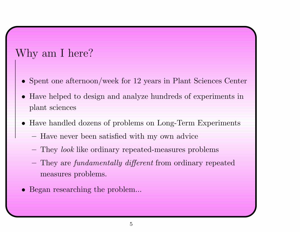
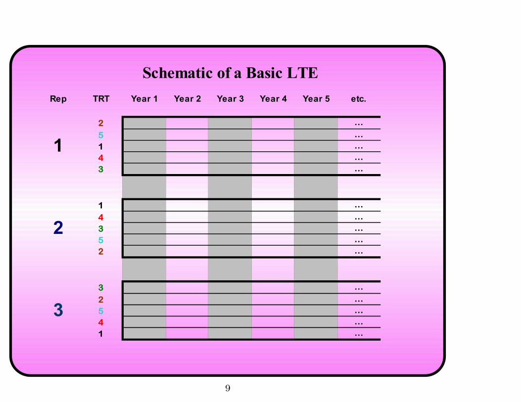
Goals of this talk
1. Review “standard practice” in analysis of long-term
experiments
2. Explain why none of these methods are correct for Long-Term
Experiments
3. Offer suggestions for improving analysis
• Explain why nothing can work perfectly
4. Place blame on the design of the experiment
5. Offer suggestions for improving design of long-term experiments
Familiarity with general ANOVA concepts is assumed.
6

What is a LTE?
Long-Term Experiments (LTEs) are
• Conducted to compare long-term effects (e.g. sustainability) of
various “Treatments” (TRTs) on some “response(s)” (Y ):
– Soil Fertility and other properties
– Erosion
– Crop Yields
– Pest Control
• “Long” term:
– Many years (Rothamsted “classicals” > 100 years)
– A few years (“Young”, or with shorter-term goals)
7

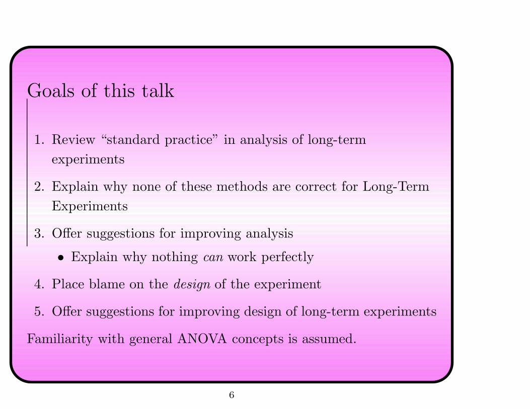
Typical Design of an LTE
• Select an experimental design (commonly RCB)
– Additional features, such as factorial treatment structure or
split-plot design, may be used as needed
• Assign treatments (TRTs) to units (plots)
– TRTs may be one-time applications, continual or varying
practices
– Tillage, chemical applications, rotations, etc.
• TRTs assigned at start of experiment never change
• Measure response on each unit (plot) repeatedly over time
– Annual (crop yield) or more often (soil/plant properties)
8
9

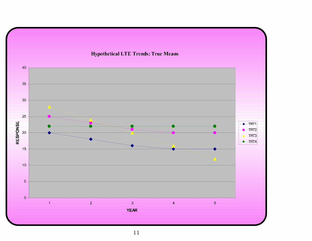
Analysis goals of a LTE
Primarily:
1. Understand differences in TRT effects over time
2. Understand how means change over time for different TRTs
These are Interaction effects between Time and TRT
10
11

Analysis goals of a LTE, cont’d
Secondarily:
1. Determine whether there is an overall time effect on the
measurements
2. Whether there are overall TRT effects on the measurements
These are Main Effects of time and TRT, respectively.
12

Data from a LTE
Special kind of repeated measures:
• Multiple measurements made over time on each experimental
unit
– Often annual, but can be any intervals
– Often equally-spaced in time, but not necessarily
• Measurements taken on all units at the same time
13

Repeated Measures Analysis
Three approaches used in most cases:
1. Derived Variables
2. Multivariate Analysis
3. Modeling of Serial Correlation
(a) Split Plot (assuming correlation is constant)
(b) Other models (allowing correlation to vary)
14
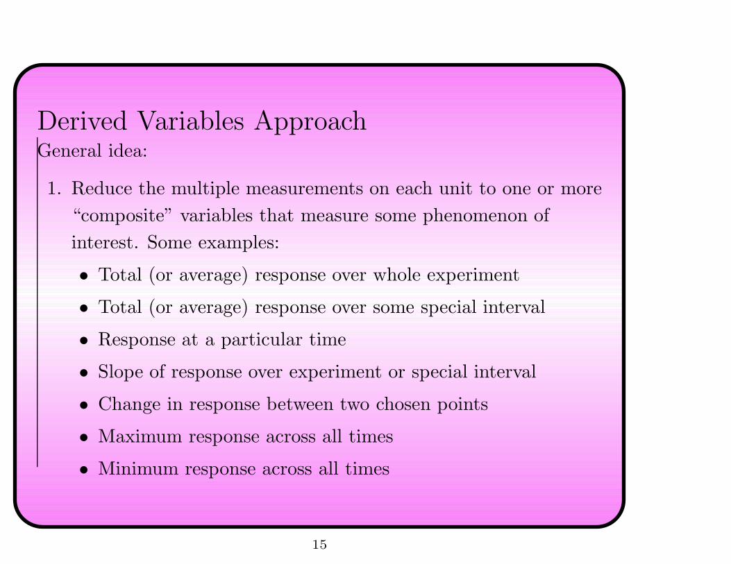
Derived Variables ApproachGeneral idea:
1. Reduce the multiple measurements on each unit to one or more
“composite” variables that measure some phenomenon of
interest. Some examples:
• Total (or average) response over whole experiment
• Total (or average) response over some special interval
• Response at a particular time
• Slope of response over experiment or special interval
• Change in response between two chosen points
• Maximum response across all times
• Minimum response across all times
15
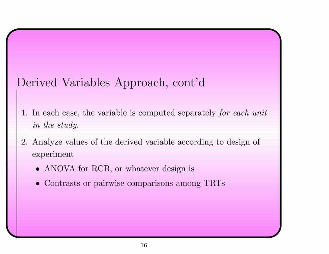
Derived Variables Approach, cont’d
1. In each case, the variable is computed separately for each unit
in the study.
2. Analyze values of the derived variable according to design of
experiment
• ANOVA for RCB, or whatever design is
• Contrasts or pairwise comparisons among TRTs
16

Derived Variables Approach, cont’d
Advantages:
• Easy to do analysis
• Easy to interpret results
Disadvantages:
• No formal F -test of Time, TRT, Time*TRT
• Possibly very many tests if numerous different derived variables
are considered
– Inflated risk of Type I Error (false rejection)
• Reducing data to simpler forms may reduce power for some
comparisons
17
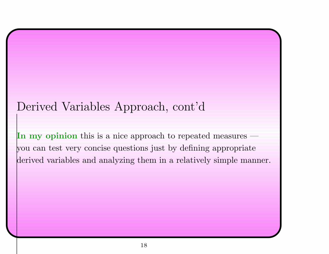
Derived Variables Approach, cont’d
In my opinion this is a nice approach to repeated measures —
you can test very concise questions just by defining appropriate
derived variables and analyzing them in a relatively simple manner.
18

*Multivariate Analysis Approach
• Responses Y1, Y2, . . . , Yr for measurements over r times
• Multivariate ANOVA (MANOVA): Simultaneously model
Y1, Y2, . . . , Yr according to design of experiment
– Effects of TRTs are compared on “best” combinations of
response variables as determined by correlation structure
among them
– A single test simultaneously compares TRTs at all times
– Separate tests at each time are often done as a follow-up
19
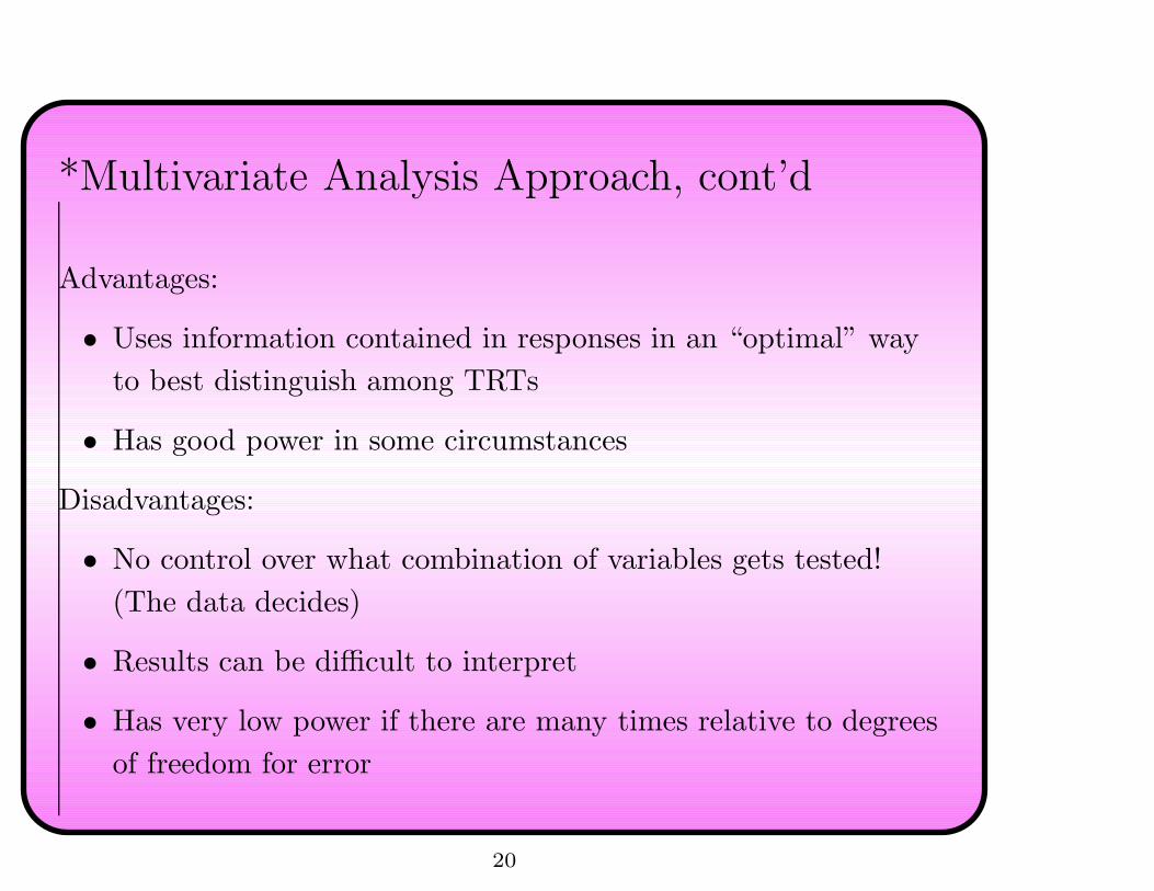
*Multivariate Analysis Approach, cont’d
Advantages:
• Uses information contained in responses in an “optimal” way
to best distinguish among TRTs
• Has good power in some circumstances
Disadvantages:
• No control over what combination of variables gets tested!
(The data decides)
• Results can be difficult to interpret
• Has very low power if there are many times relative to degrees
of freedom for error
20

*Multivariate Analysis Approach, cont’d
In my opinion this is not a very useful method of analysis for
most repeated measures problems.
(It is not often used.)
21

Modeling the Serial Correlation
“Serial correlation” = correlation over time.
Cochran (1939) recognized that LTE data “looks like” data from a
split plot:
22

23

Modeling the Serial Correlation, cont’d
Cochran (1939) also recognized that
• Measurements taken close together in time are often more
closely related to each other than measurements taken farther
apart.
• Therefore, serial correlation is higher for neighboring times
than distant times.
24

Modeling the Serial Correlation, cont’d
25
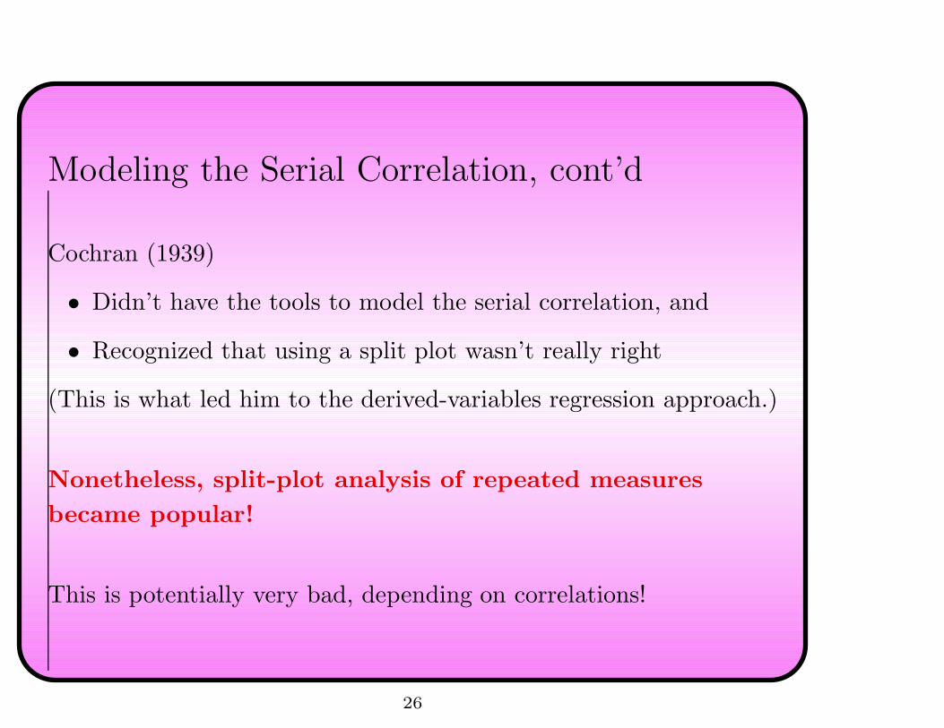
Modeling the Serial Correlation, cont’d
Cochran (1939)
• Didn’t have the tools to model the serial correlation, and
• Recognized that using a split plot wasn’t really right
(This is what led him to the derived-variables regression approach.)
Nonetheless, split-plot analysis of repeated measures
became popular!
This is potentially very bad, depending on correlations!
26

Modeling the Serial Correlation, cont’d
We now have tools to model serial correlations, so there is no
longer any need to analyze repeated measures as split plots.
PROC MIXED in SAS can fit many different correlation models (So
many, in fact, that now you need to know how to choose!)
repeated TIME / subject=_________ type=___;
27
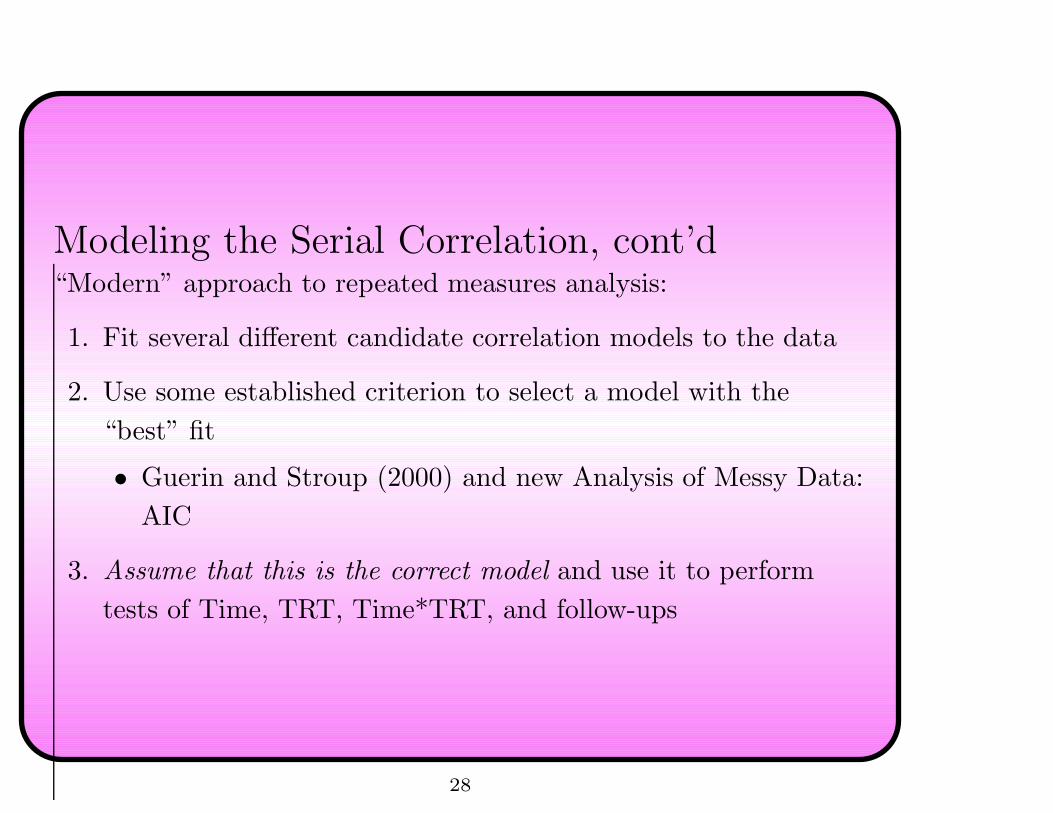
Modeling the Serial Correlation, cont’d“Modern” approach to repeated measures analysis:
1. Fit several different candidate correlation models to the data
2. Use some established criterion to select a model with the
“best” fit
• Guerin and Stroup (2000) and new Analysis of Messy Data:
AIC
3. Assume that this is the correct model and use it to perform
tests of Time, TRT, Time*TRT, and follow-ups
28
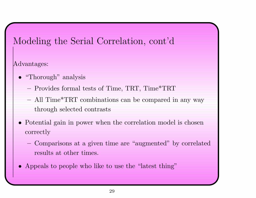
Modeling the Serial Correlation, cont’d
Advantages:
• “Thorough” analysis
– Provides formal tests of Time, TRT, Time*TRT
– All Time*TRT combinations can be compared in any way
through selected contrasts
• Potential gain in power when the correlation model is chosen
correctly
– Comparisons at a given time are “augmented” by correlated
results at other times.
• Appeals to people who like to use the “latest thing”
29
Modeling the Serial Correlation, cont’d
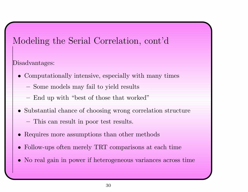
Disadvantages:
• Computationally intensive, especially with many times
– Some models may fail to yield results
– End up with “best of those that worked”
• Substantial chance of choosing wrong correlation structure
– This can result in poor test results.
• Requires more assumptions than other methods
• Follow-ups often merely TRT comparisons at each time
• No real gain in power if heterogeneous variances across time
30
Modeling the Serial Correlation, cont’d
In my opinion this is a useful procedure in a limited number of
problems
• When a formal test of Time*TRT is needed
• When an understanding of the serial correlation is desired
• When no derived variables are interesting
31

Interim Conclusion
There are several viable methods for analyzing repeated-measures
data.
Each has benefits and drawbacks.
Each has been used in published analyses of LTEs
32

Each of these methods is wrong for LTEs!
33
Fundamental Problem with LTE Data
You are looking for this:
34

35

Fundamental Problem with LTE Data
But what you have is this:
36

37

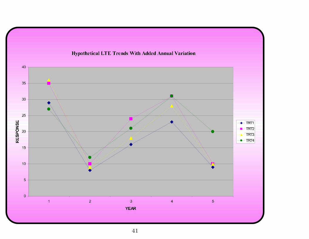
Fundamental Problem with LTE Data, cont’d
In an LTE, random annual variations in environments
affect ALL units simultaneously.
• All units’ responses rise and fall in unison
• Random interactions between TRTs and Environments further
obscure treatment comparisons over time
• Violates primary assumption of all repeated measures analyses:
Units must respond independently of one another
– Often the most critical assumption in an analysis!
38

Fundamental Problem with LTE Data, cont’d
None of the standard repeated measures analyses can distinguish
• “Fixed” effects of time: repeatable, real trends
• “Random” effects of time: uncontrollable, unrepeatable
fluctuations
Instead they combine the effects and test them simultaneously.
Analyses (Poehlman 2003, Bailey et al. 1996) show that random
effects can overwhelm fixed effects.
• How do you interpret a significant F-test?
39

Can this be fixed?
No...
⌢
• Flaw is in design of experiment
• Design lacks replication of year environments
– Fixed and Random effects are “confounded” (inseparable)
– No way to distinguish them without further assumptions
– Conclusions limited to observed sequence of years!
(Try predicting means at year 2!)
40
41
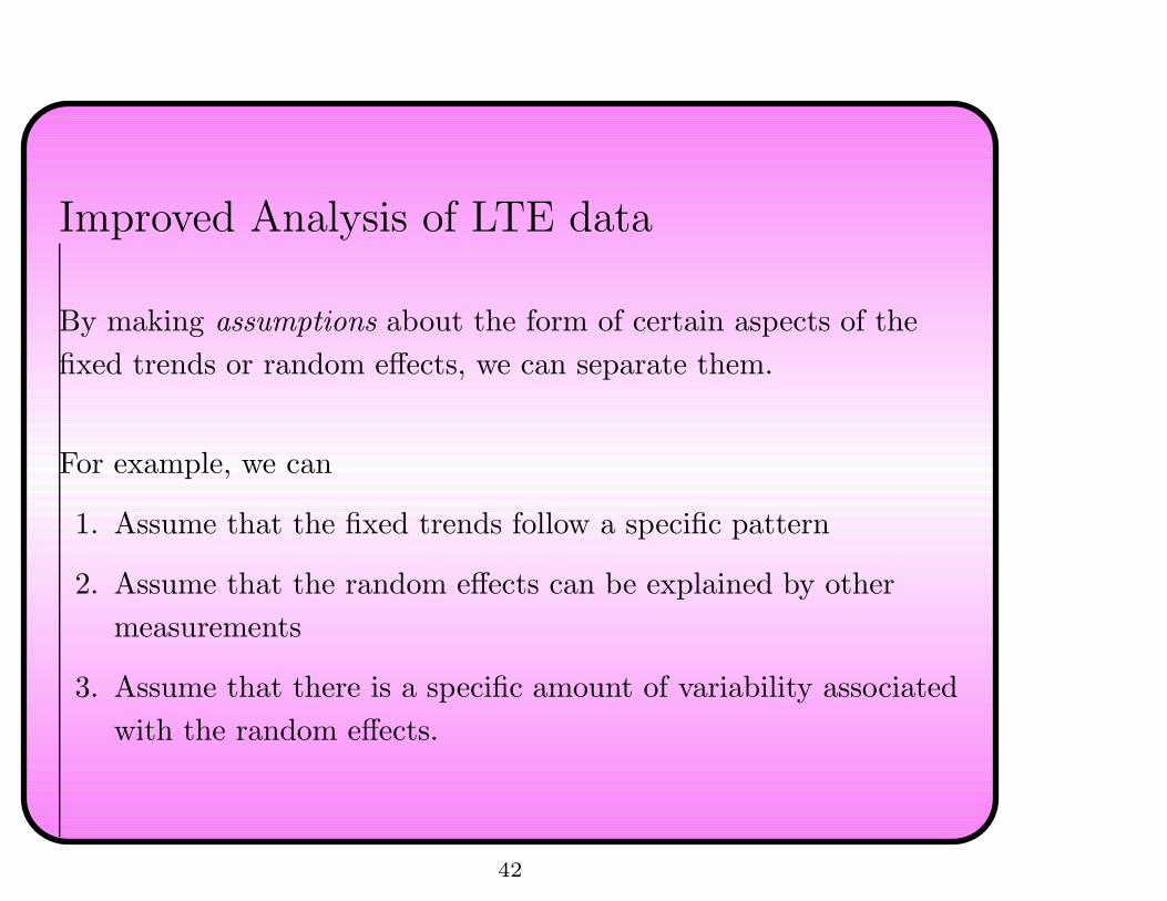
Improved Analysis of LTE data
By making assumptions about the form of certain aspects of the
fixed trends or random effects, we can separate them.
For example, we can
1. Assume that the fixed trends follow a specific pattern
2. Assume that the random effects can be explained by other
measurements
3. Assume that there is a specific amount of variability associated
with the random effects.
42

Improved Analysis of LTE data, cont’d
1. Assume that the fixed trends follow a specific pattern
• Assume that the mean trends over time for each treatment
follow some known equation
– Linear regression
– Polynomial regression
– Exponential decay
– Something else
• Assume that any deviation from the assumed model is due to
randomness (and not failure of the model)
– Use variation around fitted equation to estimate variance
associated with random effects
• Incorporate this into method that models serial correlation
43

Improved Analysis of LTE data, cont’d1. Assume that the fixed trends follow a specific pattern
Example: Let’s see whether we can extract Truth from Data:
44

45

46

Improved Analysis of LTE data, cont’d1. Assume that the fixed trends follow a specific pattern
Example: Let’s see whether we can extract Truth from Data:
Generated data from these latter means:
• Four reps
• Added a little bit of block variability
• Added a little bit of plot variability
Will assume linear trends for all treatments
47

*Improved Analysis of LTE data, cont’d1. Assume that the fixed trends follow a specific pattern
ANOVA for this analysis (start with standard split plot):
Source DF
Block (b− 1) b = # blocks (4 here)
TRT (t− 1) t = # TRTs (4 here)
Block*TRT (b− 1)(t− 1)
Year (r − 1) r = # times (5 here)
Year*TRT (r − 1)(t− 1)
Error t(b− 1)(r − 1)
Total btr − 1
48

*Improved Analysis of LTE data, cont’d1. Assume that the fixed trends follow a specific pattern
Add assumed time pattern
Source DF
Block (b − 1) “Time” = numerical variable
TRT (t − 1) representing fixed time levels
Block*TRT (b − 1)(t − 1) for linear trend
Time 1
Year (r − 2) “Year” = Class variable
Time*TRT (t − 1) representing random effects
Year*TRT (r − 2)(t − 1) of environments
Error t(b − 1)(r − 1)
Total btr − 1
49
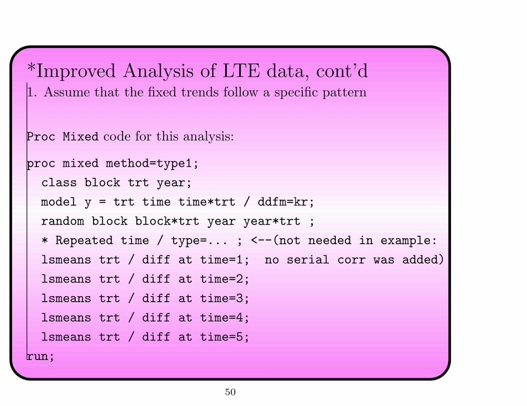
*Improved Analysis of LTE data, cont’d1. Assume that the fixed trends follow a specific pattern
Proc Mixed code for this analysis:
proc mixed method=type1;
class block trt year;
model y = trt time time*trt / ddfm=kr;
random block block*trt year year*trt ;
* Repeated time / type=... ; <--(not needed in example:
lsmeans trt / diff at time=1; no serial corr was added)
lsmeans trt / diff at time=2;
lsmeans trt / diff at time=3;
lsmeans trt / diff at time=4;
lsmeans trt / diff at time=5;
run;
50

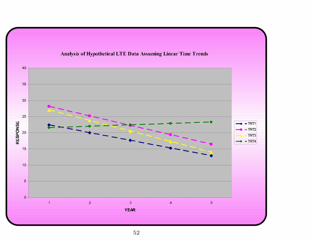
Improved Analysis of LTE data, cont’d1. Assume that the fixed trends follow a specific pattern
Results of this analysis:
Type 1 Analysis of Variance
Error
Source DF F Value Pr > F
trt 8.8832 3.93 0.0486
time 3 0.37 0.5862
time*trt 9 4.44 0.0356
51
52

53

Improved Analysis of LTE data, cont’d1. Assume that the fixed trends follow a specific pattern
Advantages:
• Interpretation is straightforward
• Can be quite accurate if chosen equation is right (or close)
Disadvantages:
• When chosen equation is wrong:
– Get wrong comparisons of means
– Lose power for tests (error terms inflated)
• Need to model serial correlation
54

Improved Analysis of LTE data, cont’d
2. Assume that “Random” effects can be explained
(Cochran 1939, [Fisher], Patterson 1953, and others)
• Add covariates for each time to explain “random” variation
– Rainfall (overall or at certain periods within season)
– Solar radiation/cloud cover
– Pest incidence
– Something else
• Use these as additional fixed effects in serial correlation models
• Add interactions with TRT
• Assume that all random variation is explained by covariate(s)
55

*Improved Analysis of LTE data, cont’d2. Assume that “Random” effects can be explained
ANOVA for this analysis (starting with standard split plot):
56

Source DF
Block (b− 1) X1 = First Covariate
TRT (t− 1) X2 = Second Covariate
Block*TRT (b− 1)(t− 1) (more are possible)
X1 1
X2 1 Year, Year*TRT now fixed
Year (r − 1) − 2 ← Lose DF to covariates
X1 ∗ TRT 1
X2 ∗ TRT 1
Year*TRT (r − 1)(t − 1) − 2 ← Lose DF to covariates
Error t(b− 1)(r − 1)
Total btr − 1
57

*Improved Analysis of LTE data, cont’d2. Assume that “Random” effects can be explained
Proc Mixed code for this analysis:
proc mixed data=set1;
class block trt year;
model y = trt X1 X2 Year X1*trt X2*trt Year*trt/ddfm=kr;
random block block*trt;
Repeated Year / subject=block*trt type=___;
lsmeans trt / diff at means;
lsmeans trt / diff at (x1,x2)=(___,___);
run;
58

Improved Analysis of LTE data, cont’d2. Assume that “Random” effects can be explained
Advantages:
• “X*TRT” effects can help in understanding TRT reactions to
environmental factors
Disadvantages:
• Covariates not likely to capture all random variability
– Remainder contaminates fixed effect (F-tests reject too
often)
• Still need to model serial correlation
• Must plan ahead to measure covariates
(or be able to obtain them retrospectively)
59
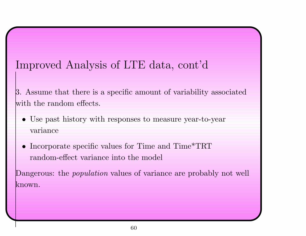
Improved Analysis of LTE data, cont’d
3. Assume that there is a specific amount of variability associated
with the random effects.
• Use past history with responses to measure year-to-year
variance
• Incorporate specific values for Time and Time*TRT
random-effect variance into the model
Dangerous: the population values of variance are probably not well
known.
60

Recommendation
Use whatever you are most comfortable with for your problem!
In general a model for the mean trend is probably safest and
easiest, as long as a reasonable model can be found.
(Can combine this with other assumptions.)
NOTHING works exactly right. Ignoring the problem is even worse.
61

How can this problem be avoided?
Problem is a lack of replication of the time sequence
• First time measurements all subjected to year 1 environments
• Second time measurements all subjected to year 2 environments
• And so forth
Alleged “replication” (blocks) are really just subsampling the same
time sequence (pseudo-replication).
62

SOLUTION:
REPLICATE LTE IN TIME!
63

This isn’t new...
From “Instructions for Authors” for Agronomy Journal
(www.asa-cssa-sssa.org):
“Field experiments that are sensitive to
environmental interactions and in which the crop
environment is not rigidly controlled or monitored,
such as studies on crop yield and yield components,
usually should be repeated (over time or space, or
both) to demonstrate that similar results can, or
cannot, be obtained in another environmental
regime.”
Here “environmental regime” = sequence of years!
64
The Facts
If you want to make statements about time sequences
other than the particular one you observe, then you must
obtain replicate time sequences.
Who wants to wait until an LTE is over to start another one???
65

The Compromise
The Staggered-Start Experiment
Smith (1979), Preece (1986), McRae and Ryan (1996), Davies
(1996)
66

67
Analysis of a Staggered-Start LTE
Derived Variables analysis is “nearly legitimate”
• Effects of year sequences are different in different blocks
• Responses for units in different blocks not quite independent,
but not heavily correlated.
• Tests probably not badly affected
(Results as if independent units)
68

Analysis of a Staggered-Start LTE
Modeling the serial correlation can be done with amended starting
ANOVA
• Separate effects for Year (random) and Time (Fixed)
• Certain interactions combine to form error terms
• Works out to be like a weird combination of Latin Square and
Strip plot
69

*Analysis of a Staggered-Start LTE
Source DF Now
Block (b− 1) # Years > # Times
Year (y − 1) y = # years
Time (r − 1) y = t + b− 1
Blk*Year*Time (r − 2)(b− 2)− 1
TRT (t− 1)
Block*TRT (b− 1)(t− 1)
Year*TRT (y − 1)(t− 1)
Time*TRT (r − 1)(t− 1)
Error (t− 1)((r − 2)(b− 2)− 1)
Total btr − 1
70

Analysis of a Staggered-Start LTE
Returning to hypothetical example: Recreated data
• Used same means as before
• Added variability for Year, Year*TRT
• Added block and plot variability
• Ran the analysis
71

72

*Analysis of a Staggered-Start LTE
proc mixed data=set1;
class block trt year time;
model y = trt time time*trt / ddfm=kr;
random block year block*year*trt block*trt year*trt;
* Repeated time / type=... <--- not needed here because
lsmeans TRT*TIME / diff; no serial corr
run;
73
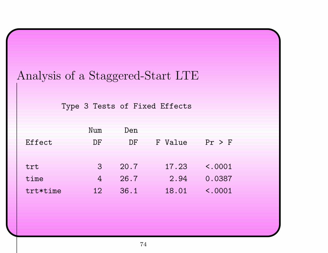
Analysis of a Staggered-Start LTE
Type 3 Tests of Fixed Effects
Num Den
Effect DF DF F Value Pr > F
trt 3 20.7 17.23 <.0001
time 4 26.7 2.94 0.0387
trt*time 12 36.1 18.01 <.0001
74

75

76

Conclusions
1. LTEs are generally designed wrong
2. This flaw invalidates ALL standard analyses
3. Analyses can be partially salvaged by added
assumptions
4. Staggered-Start design circumvents problem!
Slides from talk available at
www-personal.ksu.edu/~loughin/STATPAGE.html
77

*References
1. Bailey, T. B., Swan, J. B., Higgs, R. L., and Paulson, W. H. (1996),
“Long-Term Tillage Effects on Continuous Corn Yields,”Proceedings
of the 8th Annual Conference on Applied Statistics in Agriculture,
Manhattan, KS: Kansas State University, 18–32.
2. Cochran, W. G. (1939), “Long-Term Agricultural Experiments”
(with discussion), Journal of the Royal Statistical Society, 6[Suppl.],
104–148.
3. Davies, A. (1996), “Long-Term Forage and Pasture Investigations in
the UK,” Canadian Journal of Plant Science, 76, 573–579.
4. Guerin, L. and Stroup, W. W. (2000), “A Simulation Study to
Evaluate PROC MIXED Analysis of Repeated Measures Data,”
Proceedings of the 12th Annual Conference on Applied Statistics in
Agriculture, Manhattan, KS: Kansas State University, 170–203.
78

*References, cont’d
5. McRae, K. B. and Ryan, D. A. J. (1996), “Design and Planning of
Long-Term Experiments,” Canadian Journal of Plant Science, 76,
595–601.
6. Patterson, H. D. (1953), ”The Analysis of the Results of a Rotation
Experiment on the Use of Straw and Fertilisers,” Journal of
Agricultural Science, Cambridge, 43, 77–88.
7. Poehlman, M. J. (2003), ”Design and Analysis of Long-Term Field
Trials with Annual Measurements,” unpublished M.S. report,
Department of Statistics, Kansas State University.
8. Preece, D. A. (1986), “Some General Principles of Crop Rotation
Experiments,” Experimental Agriculture, 22, 187–198.
79

*References, cont’d
9. Smith, A. (1979), “Changes in Botanical Composition and Yield in a
Long-Term Experiment,” pages 69–75 in Changes in Sward
Composition and Productivity, eds. A. H. Charles and R. J. Hagger,
Reading, UK: British Grassland Society.
80
Recommended