BCOR 1020Business Statistics
Lecture 11 – February 21, 2008

Overview
• Chapter 6 – Discrete Distributions– Poisson Distribution– Linear Transformations

Chapter 6 – Poisson Distribution
Poisson Processes:• If the number of “occurrences” of interest on a given
continuous interval (of time, length, etc.) are being counted, we say we have an approximate Poisson Process with parameter > 0 (occurrences per unit length/time) if the following conditions are satisfied…
1) The number of “occurrences” in non-overlapping intervals are independent.
2) The probability of exactly one “occurrences” in a sufficiently short interval of length h is h. (i.e. If the interval is scaled by h, we also scale the parameter by h.)
3) The probability of two or more “occurrences” in a sufficiently short interval is essentially zero. (i.e. there are no simultaneous “occurrences”.)
Chapter 6 – Poisson Distribution
Poisson Distribution:• The Poisson distribution describes the number of
occurrences within a randomly chosen unit of time or space.
• For example, within a minute, hour, day, square foot, or linear mile.
If X denotes the number of “occurrences” of interest observed on a given interval of length 1 unit of a Poisson Process with parameter > 0, then we say that X has the Poisson distribution with parameter .

Chapter 6 – Poisson DistributionPoisson Distribution:• Called the model of arrivals, most Poisson applications
model arrivals per unit of time.• The events occur randomly and independently
over a continuum of time or space:
One Unit One Unit One Unit of Time of Time of Time |---| |---| |---|• • •• • • • •••• • • • •• • • ••• • • •
Flow of Time
• Each dot (•) is an occurrence of the event of interest.

Chapter 6 – Poisson Distribution• Let X = the number of events per unit of time.• X is a random variable that depends on when the
unit of time is observed.• For example, we could get X = 3 or X = 1 or
X = 5 events, depending on where the randomly chosen unit of time happens to fall.
One Unit One Unit One Unit of Time of Time of Time |---| |---| |---|• • •• • • • •••• • • • •• • • ••• • • •
Flow of Time
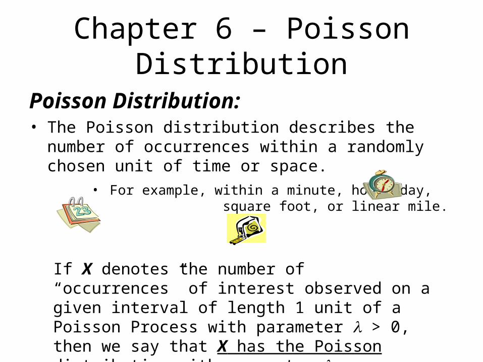
Chapter 6 – Poisson Distribution• Arrivals (e.g., customers, defects, accidents) must
be independent of each other.• Some examples of Poisson models in which
assumptions are sufficiently met are:
• X = number of customers arriving at a bank ATM in a given minute.
• X = number of file server virus infections at a data center during a 24-hour period.
• X = number of blemishes per sheet of white bond paper.
Chapter 6 – Poisson Distribution
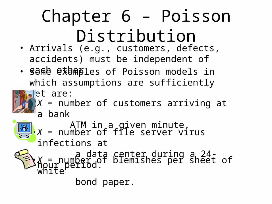
Poisson Processes:
represents the mean number of events (occurrences) per unit of time or space.
• The unit of time should be short enough that the mean arrival rate is not large (< 20).
• To make smaller, convert to a smaller time unit (e.g., convert hours to minutes).
• The Poisson model’s only parameter is (Greek letter “lambda”).

Chapter 6 – Poisson Distribution
Poisson Processes:
• The number of events that can occur in a given unit of time is not bounded, therefore X has no obvious limit.
• However, Poisson probabilities taper off toward zero as X increases.
• The Poisson distribution is sometimes called the model of rare events.
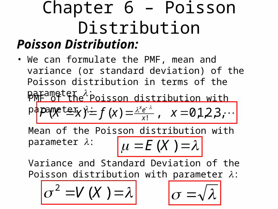
Chapter 6 – Poisson Distribution
Poisson Distribution:• We can formulate the PMF, mean and variance (or
standard deviation) of the Poisson distribution in terms of the parameter :
,3,2,1,0,)()( ! xxfxXP x
ex PMF of the Poisson distribution with parameter :
)(XE
)(2 XV
Mean of the Poisson distribution with parameter :
Variance and Standard Deviation of the Poisson distribution with parameter :

Chapter 6 – Poisson Distribution
Parameters = mean arrivals per unit of time or space
Range X = 0, 1, 2, ... (no obvious upper limit)
Mean
St. Dev.
Random data Use Excel’s Tools | Data Analysis | Random Number Generation
Comments Always right-skewed, but less so for larger .
( )!
xeP x
x

Chapter 6 – Poisson Distribution
• Poisson Processes:
Poisson distributions are always right-skewed but become less skewed and more bell-shaped as increases.
0.00
0.05
0.10
0.15
0.20
0.25
0.30
0.35
0.40
0.45
0.50
0 4 8 12 16
Number of Calls
= 0.8
0.00
0.05
0.10
0.15
0.20
0.25
0.30
0.35
0 4 8 12 16
Number of Calls
= 1.6
0.00
0.02
0.04
0.06
0.08
0.10
0.12
0.14
0.16
0.18
0 4 8 12 16
Number of Calls
= 6.4
Chapter 6 – Poisson Distribution
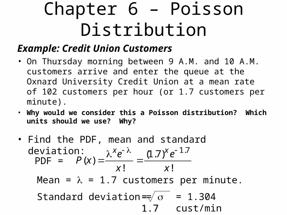
Example: Credit Union Customers• On Thursday morning between 9 A.M. and 10 A.M.
customers arrive and enter the queue at the Oxnard University Credit Union at a mean rate of 102 customers per hour (or 1.7 customers per minute).
• Why would we consider this a Poisson distribution? Which units should we use? Why?
• Find the PDF, mean and standard deviation:
PDF = 1.7(1.7)
( )! !
x xe eP x
x x
Mean = = 1.7 customers per minute.
Standard deviation = = 1.7= 1.7 = 1.304 cust/min

Chapter 6 – Poisson Distribution
• Example: Credit Union Customers• Here is the Poisson probability
distribution for = 1.7 customers per minute on average.
xPDF
P(X = x)CDF
P(X x)
0 .1827 .1827
1 .3106 .4932
2 .2640 .7572
3 .1496 .9068
4 .0636 .9704
5 .0216 .9920
6 .0061 .9981
7 .0015 .9996
8 .0003 .9999
9 .0001 1.0000
• Note that x represents the number of customers.
• For example, P(X=4) is the probability that there are exactly 4 customers in the bank.
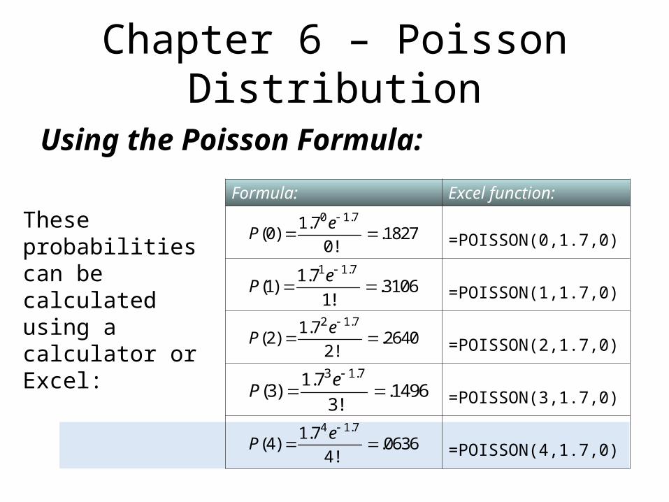
Chapter 6 – Poisson Distribution
Using the Poisson Formula:
These probabilities can be calculated using a calculator or Excel:
Formula: Excel function:
=POISSON(0,1.7,0)
=POISSON(1,1.7,0)
=POISSON(2,1.7,0)
=POISSON(3,1.7,0)
=POISSON(4,1.7,0)
3 1.71.7(3) .1496
3!
eP
4 1.71.7(4) .0636
4!
eP
2 1.71.7(2) .2640
2!
eP
1 1.71.7(1) .3106
1!
eP
0 1.71.7(0) .1827
0!
eP

Chapter 6 – Poisson Distribution
• Here are the graphs of the distributions:
0.00
0.05
0.10
0.15
0.20
0.25
0.30
0.35
0 1 2 3 4 5 6 7 8 9
Number of Customer Arrivals
Pro
bab
ility
0.00
0.10
0.20
0.30
0.40
0.50
0.60
0.70
0.80
0.90
1.00
0 1 2 3 4 5 6 7 8 9
Number of Customer Arrivals
Pro
bab
ility
Poisson PDF for = 1.7 Poisson CDF for = 1.7
• The most likely event is 1 arrival (P(1)=.3106 or 31.1% chance).
• This will help the credit union schedule tellers.
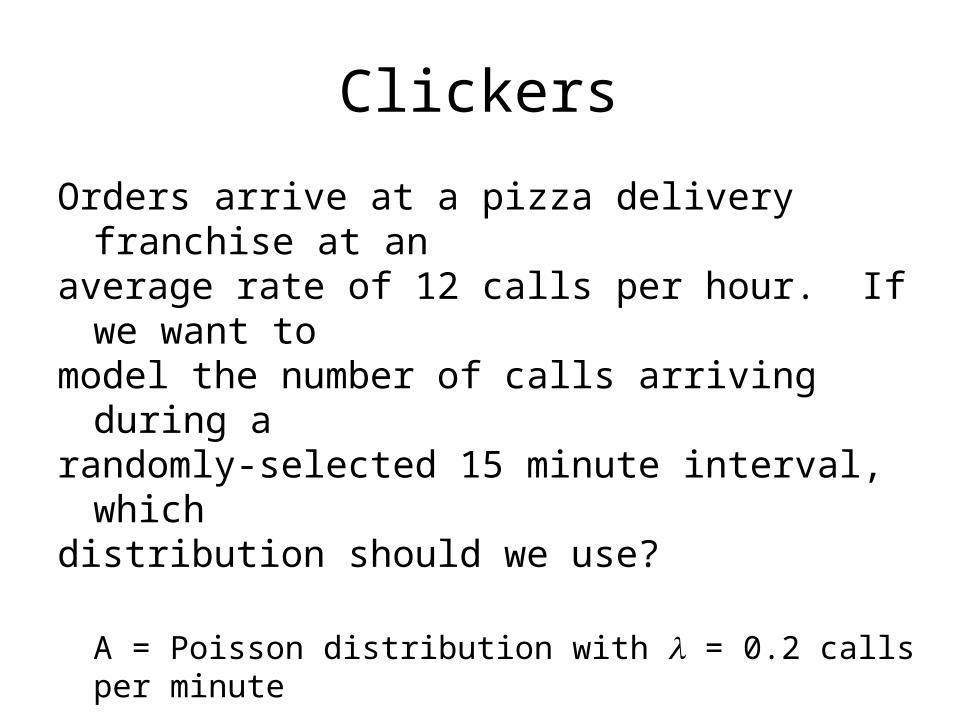
Clickers
Orders arrive at a pizza delivery franchise at an average rate of 12 calls per hour. If we want to model the number of calls arriving during a randomly-selected 15 minute interval, which distribution should we use?
A = Poisson distribution with = 0.2 calls per minute
B = Poisson distribution with = 0.8 calls per 15 minutes
C = Poisson distribution with = 3 calls per 15 min.
D = Poisson distribution with = 12 calls per hour

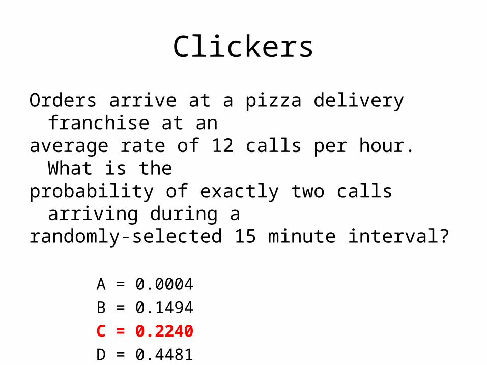
Clickers
Orders arrive at a pizza delivery franchise at an average rate of 12 calls per hour. What are the mean and standard deviation of the number of calls arriving during a randomly-selected 15 minute interval?
A = = 3 and = 1.73
B = = 3 and = 3
C = = 12 and = 3.46
D = = 12 and = 12
Clickers
Orders arrive at a pizza delivery franchise at an average rate of 12 calls per hour. What is the probability of exactly two calls arriving during a randomly-selected 15 minute interval?
A = 0.0004
B = 0.1494
C = 0.2240
D = 0.4481
Chapter 6 – Poisson Distribution
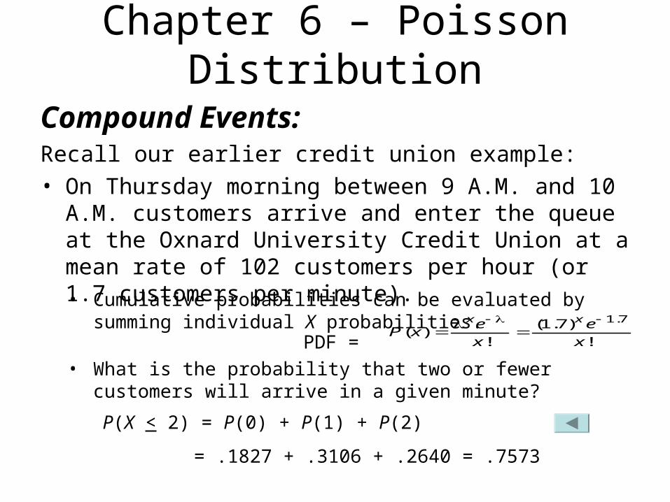
Compound Events: Recall our earlier credit union example: • On Thursday morning between 9 A.M. and 10 A.M.
customers arrive and enter the queue at the Oxnard University Credit Union at a mean rate of 102 customers per hour (or 1.7 customers per minute). • Cumulative probabilities can be evaluated by summing
individual X probabilities.
• What is the probability that two or fewer customers will arrive in a given minute?
= .1827 + .3106 + .2640 = .7573
P(X < 2) = P(0) + P(1) + P(2)
PDF =
1.7(1.7)( )
! !
x xe eP x
x x
Chapter 6 – Poisson Distribution
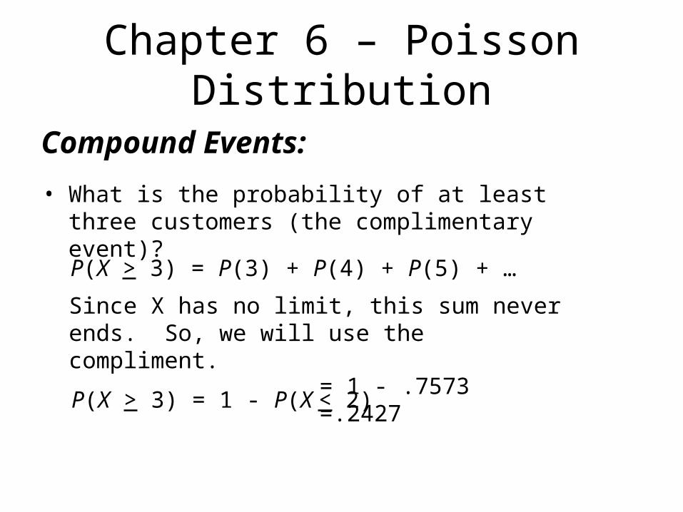
Compound Events:
• What is the probability of at least three customers (the complimentary event)?
= 1 - .7573 =.2427 P(X > 3) = 1 - P(X < 2)
P(X > 3) = P(3) + P(4) + P(5) + …
Since X has no limit, this sum never ends. So, we will use the compliment.

Clickers
Orders arrive at a pizza delivery franchise at an average rate of 12 calls per hour. What is the probability that more than two calls arrive during a randomly-selected 15 minute interval?
A = 0.0498
B = 0.1494
C = 0.2240
D = 0.4232
E = 0.5768

Chapter 6 – Poisson Distribution
Recognizing Poisson Applications:• Can you recognize a Poisson situation?
• Look for arrivals of “rare” independent events with no obvious upper limit.
• In the last week, how many credit card applications did you receive by mail?
• In the last week, how many checks did you write?
• In the last week, how many e-mail viruses did your firewall detect?

Chapter 6 – Linear Transformations
Linear Transformations:• A linear transformation of a random variable X is
performed by adding a constant or multiplying by a constant.
Rule 1: aX+b = aX + b (mean of a transformed variable)Rule 2: aX+b = |a|X (standard deviation of a transformed variable)
• For example, consider defining a random variable Y in terms of the random variable X as follows:
baXY Where a and b are any two constants.

Chapter 6 – Linear Transformations
Example: Total Cost• The total cost of many goods is often modeled as a
function of the good produced, Q (a random variable).
Fv QC
Specifically, if there is a variable cost per unit v and a fixed cost F, then the total cost of the good, C, is given by …
where v and F are constant values.
For given values of Q, Q, v, and F, we can determine the mean and standard deviation of the total cost…
QC v
FvQC

ClickersIf Q is a random variable with mean Q = 500 units and standard deviation Q = 40 units, the variable cost is v = $35 per unit, and the fixed cost is F = $24,000, the mean of the total cost is
Determine the standard deviation of the total cost.
A) C = $35
B) C = $40
C) C = $1,400
D) C = $25,400
500,41$24000)50035( Fv QC
Recommended