Bayesian random-effects meta-analysis
made simple
Christian Rover1, Beat Neuenschwander2,
Simon Wandel2, Tim Friede1
1Department of Medical Statistics,University Medical Center Gottingen,
Gottingen, Germany
2Novartis Pharma AG,Basel, Switzerland
May 24, 2016
This project has received funding from the European Union’sSeventh Framework Programme for research, technological de-velopment and demonstration under grant agreement numberFP HEALTH 2013-602144.
C. Rover et al. Bayesian meta-analysis made simple May 24, 2016 1 / 22
Overview
Meta analysis
example
the random-effects modelthe Bayesian approach
the bayesmeta package
parameter estimation
prediction
Conclusions
C. Rover et al. Bayesian meta-analysis made simple May 24, 2016 2 / 22
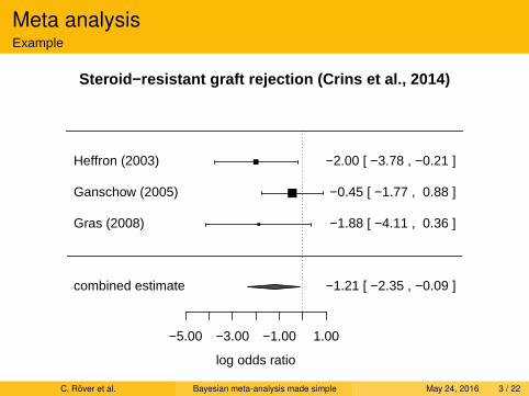
Meta analysisExample
−5.00 −3.00 −1.00 1.00
log odds ratio
Gras (2008)
Ganschow (2005)
Heffron (2003)
−1.88 [ −4.11 , 0.36 ]
−0.45 [ −1.77 , 0.88 ]
−2.00 [ −3.78 , −0.21 ]
Steroid−resistant graft rejection (Crins et al., 2014)
−1.21 [ −2.35 , −0.09 ]combined estimate
C. Rover et al. Bayesian meta-analysis made simple May 24, 2016 3 / 22
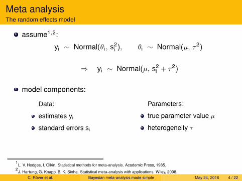
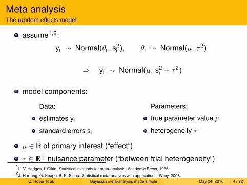
Meta analysisThe random effects model
assume1,2:
yi ∼ Normal(θi , s2i ), θi ∼ Normal(µ, τ2)
⇒ yi ∼ Normal(µ, s2i + τ2)
model components:
Data:
estimates yi
standard errors si
Parameters:
true parameter value µ
heterogeneity τ
1L. V. Hedges, I. Olkin. Statistical methods for meta-analysis. Academic Press, 1985.
2J. Hartung, G. Knapp, B. K. Sinha. Statistical meta-analysis with applications. Wiley, 2008.
C. Rover et al. Bayesian meta-analysis made simple May 24, 2016 4 / 22
Meta analysisThe random effects model
assume1,2:
yi ∼ Normal(θi , s2i ), θi ∼ Normal(µ, τ2)
⇒ yi ∼ Normal(µ, s2i + τ2)
model components:
Data:
estimates yi
standard errors si
Parameters:
true parameter value µ
heterogeneity τ
µ ∈ R of primary interest (“effect”)
τ ∈ R+ nuisance parameter (“between-trial heterogeneity”)1
L. V. Hedges, I. Olkin. Statistical methods for meta-analysis. Academic Press, 1985.2
J. Hartung, G. Knapp, B. K. Sinha. Statistical meta-analysis with applications. Wiley, 2008.
C. Rover et al. Bayesian meta-analysis made simple May 24, 2016 4 / 22
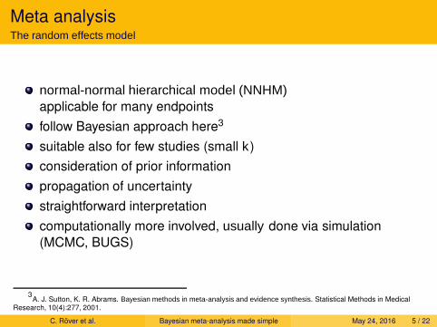
Meta analysisThe random effects model
normal-normal hierarchical model (NNHM)applicable for many endpoints
follow Bayesian approach here3
suitable also for few studies (small k)
consideration of prior information
propagation of uncertainty
straightforward interpretation
computationally more involved, usually done via simulation
(MCMC, BUGS)
3A. J. Sutton, K. R. Abrams. Bayesian methods in meta-analysis and evidence synthesis. Statistical Methods in Medical
Research, 10(4):277, 2001.
C. Rover et al. Bayesian meta-analysis made simple May 24, 2016 5 / 22
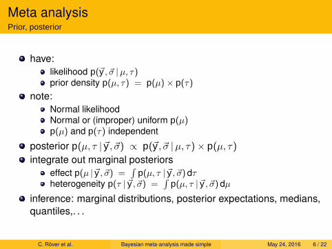
Meta analysisPrior, posterior
have:
likelihood p(~y , ~σ |µ, τ)prior density p(µ, τ) = p(µ) × p(τ)
note:
Normal likelihoodNormal or (improper) uniform p(µ)p(µ) and p(τ) independent
posterior p(µ, τ |~y , ~σ) ∝ p(~y , ~σ |µ, τ)× p(µ, τ)integrate out marginal posteriors
effect p(µ |~y , ~σ) =∫
p(µ, τ |~y , ~σ)dτheterogeneity p(τ |~y , ~σ) =
∫p(µ, τ |~y , ~σ)dµ
inference: marginal distributions, posterior expectations, medians,
quantiles,. . .
C. Rover et al. Bayesian meta-analysis made simple May 24, 2016 6 / 22
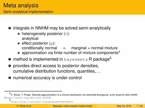
Meta analysisSemi-analytical implementation
integrals in NNHM may be solved semi-analytically
heterogeneity posterior (τ ):
analytical
effect posterior (µ):conditionally normal ⇒ marginal = normal mixture
approximation via finite number of mixture components4
method is implemented in bayesmeta R package5
provides direct access to posterior densities,
cumulative distribution functions, quantiles,. . .
numerical accuracy is under control
4C. Rover, T. Friede. Discrete approximation of a mixture distribution via restricted divergence. arXiv preprint 1602.04060
(http://arxiv.org/abs/1602.04060)5http://cran.r-project.org/package=bayesmeta
C. Rover et al. Bayesian meta-analysis made simple May 24, 2016 7 / 22
Meta analysisSemi-analytical implementation
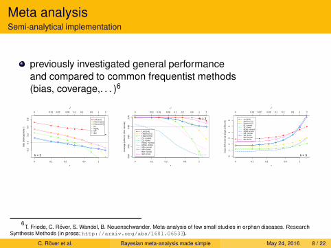
previously investigated general performance
and compared to common frequentist methods
(bias, coverage,. . . )6
Unif [0,4]HNorm (1.0)HNorm (0.5)DLREMLMPBM
k = 3
0 0.1 0.2 0.5 1
τ
0 0.01 0.02 0.05 0.1 0.2 0.5 1 2
τ2
−0.
20.
00.
20.
40.
6
bias
(he
tero
gene
ity τ
)
Unif [0,4]HNorm (1.0)HNorm (0.5)DL−normalDL−KnHaREML−normalREML−KnHaMP−normalMP−KnHaBM−normalBM−KnHa
k = 3
0 0.1 0.2 0.5 1
τ
0 0.01 0.02 0.05 0.1 0.2 0.5 1 2
τ2
0.80
0.85
0.90
0.95
1.00
cove
rage
(ef
fect
Θ, 9
5% in
terv
al)
Unif [0,4]HNorm (1.0)HNorm (0.5)DL−normalDL−KnHaREML−normalREML−KnHaMP−normalMP−KnHaBM−normalBM−KnHa
k = 3
0 0.1 0.2 0.5 1
τ
0 0.01 0.02 0.05 0.1 0.2 0.5 1 2
τ2
01
23
45
6
mea
n 95
% in
terv
al le
ngth
(ef
fect
Θ)
6T. Friede, C. Rover, S. Wandel, B. Neuenschwander. Meta-analysis of few small studies in orphan diseases. Research
Synthesis Methods (in press; http://arxiv.org/abs/1601.06533).
C. Rover et al. Bayesian meta-analysis made simple May 24, 2016 8 / 22
Meta analysisSemi-analytical implementation
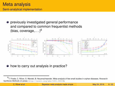
previously investigated general performance
and compared to common frequentist methods
(bias, coverage,. . . )6
Unif [0,4]HNorm (1.0)HNorm (0.5)DLREMLMPBM
k = 3
0 0.1 0.2 0.5 1
τ
0 0.01 0.02 0.05 0.1 0.2 0.5 1 2
τ2
−0.
20.
00.
20.
40.
6
bias
(he
tero
gene
ity τ
)
Unif [0,4]HNorm (1.0)HNorm (0.5)DL−normalDL−KnHaREML−normalREML−KnHaMP−normalMP−KnHaBM−normalBM−KnHa
k = 3
0 0.1 0.2 0.5 1
τ
0 0.01 0.02 0.05 0.1 0.2 0.5 1 2
τ2
0.80
0.85
0.90
0.95
1.00
cove
rage
(ef
fect
Θ, 9
5% in
terv
al)
Unif [0,4]HNorm (1.0)HNorm (0.5)DL−normalDL−KnHaREML−normalREML−KnHaMP−normalMP−KnHaBM−normalBM−KnHa
k = 3
0 0.1 0.2 0.5 1
τ
0 0.01 0.02 0.05 0.1 0.2 0.5 1 2
τ2
01
23
45
6
mea
n 95
% in
terv
al le
ngth
(ef
fect
Θ)
how to carry out analysis in practice?
6T. Friede, C. Rover, S. Wandel, B. Neuenschwander. Meta-analysis of few small studies in orphan diseases. Research
Synthesis Methods (in press; http://arxiv.org/abs/1601.06533).
C. Rover et al. Bayesian meta-analysis made simple May 24, 2016 8 / 22
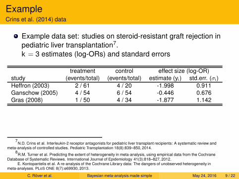
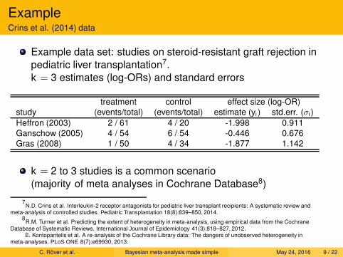
ExampleCrins et al. (2014) data
Example data set: studies on steroid-resistant graft rejection in
pediatric liver transplantation7.
k = 3 estimates (log-ORs) and standard errors
treatment control effect size (log-OR)
study (events/total) (events/total) estimate (yi ) std.err. (σi )
Heffron (2003) 2 / 61 4 / 20 -1.998 0.911
Ganschow (2005) 4 / 54 6 / 54 -0.446 0.676
Gras (2008) 1 / 50 4 / 34 -1.877 1.142
7N.D. Crins et al. Interleukin-2 receptor antagonists for pediatric liver transplant recipients: A systematic review and
meta-analysis of controlled studies. Pediatric Transplantation 18(8):839–850, 2014.8
R.M. Turner et al. Predicting the extent of heterogeneity in meta-analysis, using empirical data from the CochraneDatabase of Systematic Reviews. International Journal of Epidemiology 41(3):818–827, 2012.
E. Kontopantelis et al. A re-analysis of the Cochrane Library data: The dangers of unobserved heterogeneity inmeta-analyses. PLoS ONE 8(7):e69930, 2013.
C. Rover et al. Bayesian meta-analysis made simple May 24, 2016 9 / 22
ExampleCrins et al. (2014) data
Example data set: studies on steroid-resistant graft rejection in
pediatric liver transplantation7.
k = 3 estimates (log-ORs) and standard errors
treatment control effect size (log-OR)
study (events/total) (events/total) estimate (yi ) std.err. (σi )
Heffron (2003) 2 / 61 4 / 20 -1.998 0.911
Ganschow (2005) 4 / 54 6 / 54 -0.446 0.676
Gras (2008) 1 / 50 4 / 34 -1.877 1.142
k = 2 to 3 studies is a common scenario
(majority of meta analyses in Cochrane Database8)
7N.D. Crins et al. Interleukin-2 receptor antagonists for pediatric liver transplant recipients: A systematic review and
meta-analysis of controlled studies. Pediatric Transplantation 18(8):839–850, 2014.8
R.M. Turner et al. Predicting the extent of heterogeneity in meta-analysis, using empirical data from the CochraneDatabase of Systematic Reviews. International Journal of Epidemiology 41(3):818–827, 2012.
E. Kontopantelis et al. A re-analysis of the Cochrane Library data: The dangers of unobserved heterogeneity inmeta-analyses. PLoS ONE 8(7):e69930, 2013.
C. Rover et al. Bayesian meta-analysis made simple May 24, 2016 9 / 22
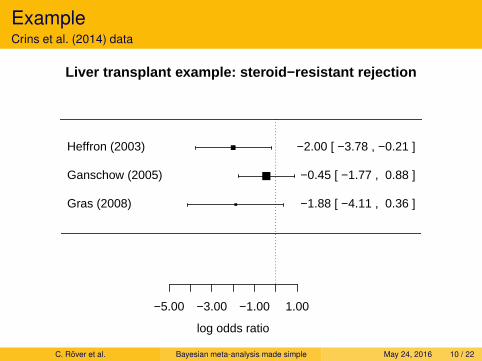
ExampleCrins et al. (2014) data
−5.00 −3.00 −1.00 1.00
log odds ratio
Gras (2008)
Ganschow (2005)
Heffron (2003)
−1.88 [ −4.11 , 0.36 ]
−0.45 [ −1.77 , 0.88 ]
−2.00 [ −3.78 , −0.21 ]
Liver transplant example: steroid−resistant rejection
C. Rover et al. Bayesian meta-analysis made simple May 24, 2016 10 / 22
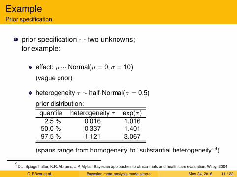
ExamplePrior specification
prior specification - - two unknowns;
for example:
effect: µ ∼ Normal(µ = 0, σ = 10)
(vague prior)
heterogeneity τ ∼ half-Normal(σ = 0.5)
prior distribution:
quantile heterogeneity τ exp(τ)2.5 % 0.016 1.016
50.0 % 0.337 1.401
97.5 % 1.121 3.067
(spans range from homogeneity to “substantial heterogeneity ”9)
9D.J. Spiegelhalter, K.R. Abrams, J.P. Myles. Bayesian approaches to clinical trials and health-care evaluation. Wiley, 2004.
C. Rover et al. Bayesian meta-analysis made simple May 24, 2016 11 / 22
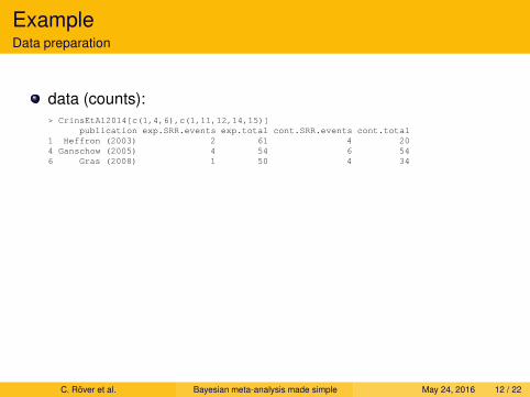
ExampleData preparation
data (counts):> CrinsEtAl2014[c(1,4,6),c(1,11,12,14,15)]
publication exp.SRR.events exp.total cont.SRR.events cont.total1 Heffron (2003) 2 61 4 204 Ganschow (2005) 4 54 6 546 Gras (2008) 1 50 4 34
C. Rover et al. Bayesian meta-analysis made simple May 24, 2016 12 / 22
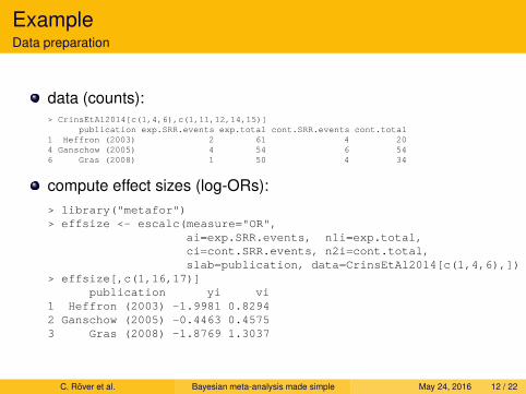
ExampleData preparation
data (counts):> CrinsEtAl2014[c(1,4,6),c(1,11,12,14,15)]
publication exp.SRR.events exp.total cont.SRR.events cont.total1 Heffron (2003) 2 61 4 204 Ganschow (2005) 4 54 6 546 Gras (2008) 1 50 4 34
compute effect sizes (log-ORs):
> library("metafor")> effsize <- escalc(measure="OR",
ai=exp.SRR.events, n1i=exp.total,ci=cont.SRR.events, n2i=cont.total,slab=publication, data=CrinsEtAl2014[c(1,4,6),])
> effsize[,c(1,16,17)]publication yi vi
1 Heffron (2003) -1.9981 0.82942 Ganschow (2005) -0.4463 0.45753 Gras (2008) -1.8769 1.3037
C. Rover et al. Bayesian meta-analysis made simple May 24, 2016 12 / 22
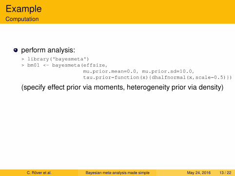
ExampleComputation
perform analysis:> library("bayesmeta")> bm01 <- bayesmeta(effsize,
mu.prior.mean=0.0, mu.prior.sd=10.0,tau.prior=function(x){dhalfnormal(x,scale=0.5)})
(specify effect prior via moments, heterogeneity prior via density)
C. Rover et al. Bayesian meta-analysis made simple May 24, 2016 13 / 22
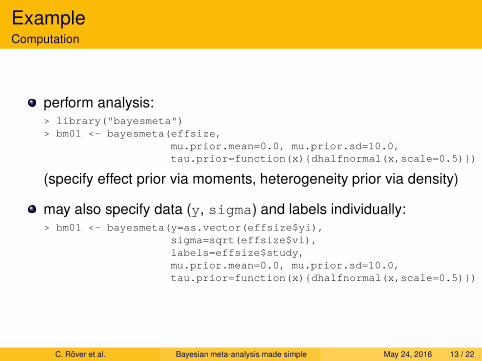
ExampleComputation
perform analysis:> library("bayesmeta")> bm01 <- bayesmeta(effsize,
mu.prior.mean=0.0, mu.prior.sd=10.0,tau.prior=function(x){dhalfnormal(x,scale=0.5)})
(specify effect prior via moments, heterogeneity prior via density)
may also specify data (y, sigma) and labels individually:> bm01 <- bayesmeta(y=as.vector(effsize$yi),
sigma=sqrt(effsize$vi),labels=effsize$study,mu.prior.mean=0.0, mu.prior.sd=10.0,tau.prior=function(x){dhalfnormal(x,scale=0.5)})
C. Rover et al. Bayesian meta-analysis made simple May 24, 2016 13 / 22
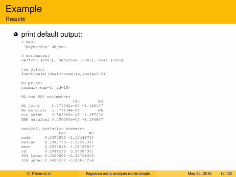
ExampleResults
print default output:> bm01’bayesmeta’ object.
3 estimates:Heffron (2003), Ganschow (2005), Gras (2008)
tau prior:function(x){dhalfnormal(x,scale=0.5)}
mu prior:normal(mean=0, sd=10)
ML and MAP estimates:tau mu
ML joint 1.771042e-04 -1.160107ML marginal 5.077174e-01 NAMAP joint 9.862966e-05 -1.157224MAP marginal 0.000000e+00 -1.194867
marginal posterior summary:tau mu
mode 0.0000000 -1.19486744median 0.3380733 -1.20525311mean 0.3920815 -1.21188547sd 0.2881225 0.5738730195% lower 0.0000000 -2.3475647395% upper 0.9406362 -0.08617254
C. Rover et al. Bayesian meta-analysis made simple May 24, 2016 14 / 22
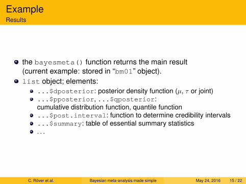
ExampleResults
the bayesmeta() function returns the main result
(current example: stored in “bm01” object).
list object; elements:
...$dposterior: posterior density function (µ, τ or joint)
...$pposterior, ...$qposterior:
cumulative distribution function, quantile function...$post.interval: function to determine credibility intervals
...$summary: table of essential summary statistics
. . .
C. Rover et al. Bayesian meta-analysis made simple May 24, 2016 15 / 22
ExampleResults
show posterior density of effect µ:mu <- seq(from=-3, to=1, length=100)plot(mu, bm01$dposterior(mu=mu), type="l",
col="blue", xlab="effect (log-OR)", ylab="probability density")
C. Rover et al. Bayesian meta-analysis made simple May 24, 2016 16 / 22
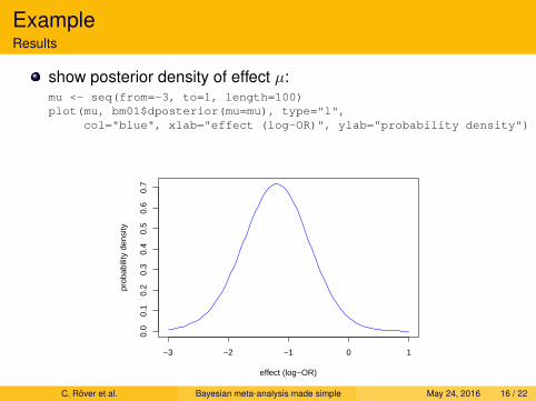
ExampleResults
show posterior density of effect µ:mu <- seq(from=-3, to=1, length=100)plot(mu, bm01$dposterior(mu=mu), type="l",
col="blue", xlab="effect (log-OR)", ylab="probability density")
−3 −2 −1 0 1
0.0
0.1
0.2
0.3
0.4
0.5
0.6
0.7
effect (log−OR)
prob
abili
ty d
ensi
ty
C. Rover et al. Bayesian meta-analysis made simple May 24, 2016 16 / 22
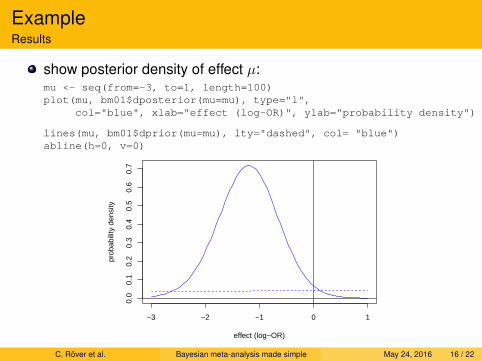
ExampleResults
show posterior density of effect µ:mu <- seq(from=-3, to=1, length=100)plot(mu, bm01$dposterior(mu=mu), type="l",
col="blue", xlab="effect (log-OR)", ylab="probability density")
lines(mu, bm01$dprior(mu=mu), lty="dashed", col= "blue")abline(h=0, v=0)
−3 −2 −1 0 1
0.0
0.1
0.2
0.3
0.4
0.5
0.6
0.7
effect (log−OR)
prob
abili
ty d
ensi
ty
C. Rover et al. Bayesian meta-analysis made simple May 24, 2016 16 / 22
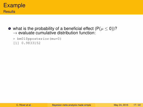
ExampleResults
what is the probability of a beneficial effect (P(µ ≤ 0))?→ evaluate cumulative distribution function:
C. Rover et al. Bayesian meta-analysis made simple May 24, 2016 17 / 22
ExampleResults
what is the probability of a beneficial effect (P(µ ≤ 0))?→ evaluate cumulative distribution function:
> bm01$pposterior(mu=0)[1] 0.9833152
C. Rover et al. Bayesian meta-analysis made simple May 24, 2016 17 / 22
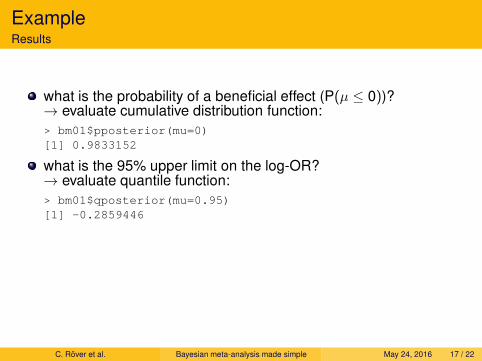
ExampleResults
what is the probability of a beneficial effect (P(µ ≤ 0))?→ evaluate cumulative distribution function:
> bm01$pposterior(mu=0)[1] 0.9833152
what is the 95% upper limit on the log-OR?→ evaluate quantile function:
> bm01$qposterior(mu=0.95)[1] -0.2859446
C. Rover et al. Bayesian meta-analysis made simple May 24, 2016 17 / 22
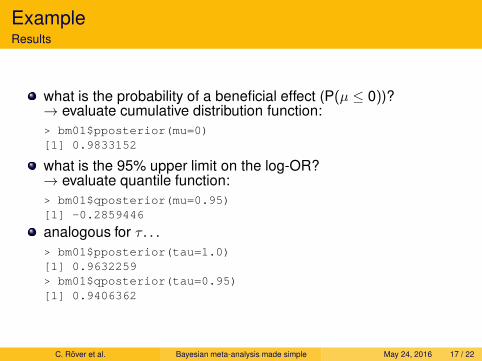
ExampleResults
what is the probability of a beneficial effect (P(µ ≤ 0))?→ evaluate cumulative distribution function:
> bm01$pposterior(mu=0)[1] 0.9833152
what is the 95% upper limit on the log-OR?→ evaluate quantile function:
> bm01$qposterior(mu=0.95)[1] -0.2859446
analogous for τ . . .
> bm01$pposterior(tau=1.0)[1] 0.9632259> bm01$qposterior(tau=0.95)[1] 0.9406362
C. Rover et al. Bayesian meta-analysis made simple May 24, 2016 17 / 22
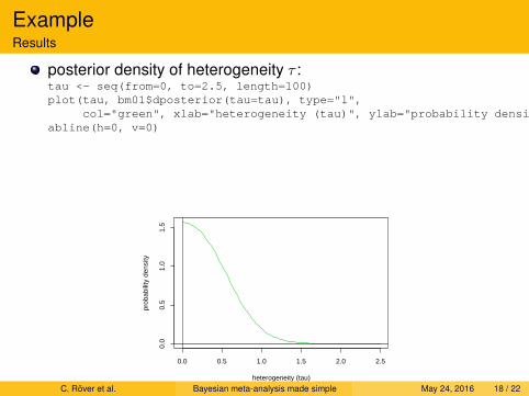
ExampleResults
posterior density of heterogeneity τ :tau <- seq(from=0, to=2.5, length=100)plot(tau, bm01$dposterior(tau=tau), type="l",
col="green", xlab="heterogeneity (tau)", ylab="probability density")abline(h=0, v=0)
0.0 0.5 1.0 1.5 2.0 2.5
0.0
0.5
1.0
1.5
heterogeneity (tau)
prob
abili
ty d
ensi
ty
C. Rover et al. Bayesian meta-analysis made simple May 24, 2016 18 / 22
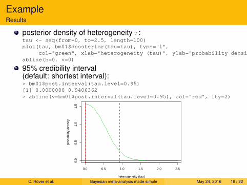
ExampleResults
posterior density of heterogeneity τ :tau <- seq(from=0, to=2.5, length=100)plot(tau, bm01$dposterior(tau=tau), type="l",
col="green", xlab="heterogeneity (tau)", ylab="probability density")abline(h=0, v=0)
95% credibility interval(default: shortest interval):> bm01$post.interval(tau.level=0.95)[1] 0.0000000 0.9406362> abline(v=bm01$post.interval(tau.level=0.95), col="red", lty=2)
0.0 0.5 1.0 1.5 2.0 2.5
0.0
0.5
1.0
1.5
heterogeneity (tau)
prob
abili
ty d
ensi
ty
C. Rover et al. Bayesian meta-analysis made simple May 24, 2016 18 / 22
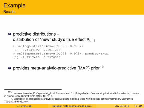
ExampleResults
predictive distributions –
distribution of “new” study’s true effect θk+1
> bm01$qposterior(mu=c(0.025, 0.975))[1] -2.3634190 -0.1011219> bm01$qposterior(mu=c(0.025, 0.975), predict=TRUE)[1] -2.7717423 0.2576317
provides meta-analytic-predictive (MAP) prior10
10B. Neuenschwander, G. Capkun-Niggli, M. Branson, and D.J. Spiegelhalter. Summarizing historical information on controls
in clinical trials. Clinical Trials 7(1):5-18, 2010.H. Schmidli et al. Robust meta-analytic-predictive priors in clinical trials with historical control information. Biometrics
70(4):1023-1032, 2014.
C. Rover et al. Bayesian meta-analysis made simple May 24, 2016 19 / 22
ExampleResults
quick sensitivity checks(uniform effect prior, very wide heterogeneity prior):bm01 <- bayesmeta(effsize,
mu.prior.mean=0.0, mu.prior.sd=10.0,tau.prior=function(x){dhalfnormal(x,scale=0.5)})
bm02 <- bayesmeta(effsize,tau.prior=function(x){dhalfnormal(x,scale=1.0)})
C. Rover et al. Bayesian meta-analysis made simple May 24, 2016 20 / 22
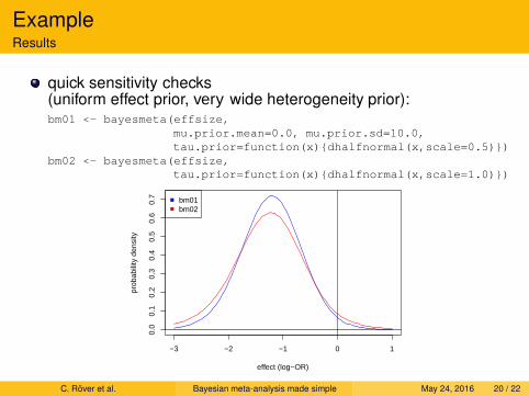
ExampleResults
quick sensitivity checks(uniform effect prior, very wide heterogeneity prior):bm01 <- bayesmeta(effsize,
mu.prior.mean=0.0, mu.prior.sd=10.0,tau.prior=function(x){dhalfnormal(x,scale=0.5)})
bm02 <- bayesmeta(effsize,tau.prior=function(x){dhalfnormal(x,scale=1.0)})
−3 −2 −1 0 1
0.0
0.1
0.2
0.3
0.4
0.5
0.6
0.7
effect (log−OR)
prob
abili
ty d
ensi
ty
bm01bm02
C. Rover et al. Bayesian meta-analysis made simple May 24, 2016 20 / 22
ExampleResults
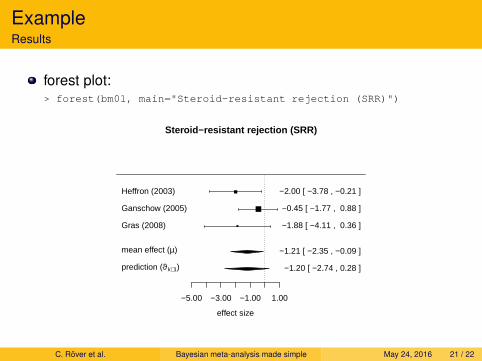
forest plot:> forest(bm01, main="Steroid-resistant rejection (SRR)")
Steroid−resistant rejection (SRR)
−5.00 −3.00 −1.00 1.00
effect size
Gras (2008)
Ganschow (2005)
Heffron (2003)
−1.88 [ −4.11 , 0.36 ]
−0.45 [ −1.77 , 0.88 ]
−2.00 [ −3.78 , −0.21 ]
−1.21 [ −2.35 , −0.09 ]mean effect (µ)
−1.20 [ −2.74 , 0.28 ]prediction (ϑk+1)
C. Rover et al. Bayesian meta-analysis made simple May 24, 2016 21 / 22

Conclusions
random-effects meta-analysis model covers wide range of cases
semi-analytical integration simplifies Bayesian meta-analysis
(esp.: no MCMC sampling necessary)
R implementation is straightforward to use
flexible prior specification
quick sensitivity analyses
includes predictive distributions
bayesmeta package available on CRAN11
11http://cran.r-project.org/package=bayesmeta
C. Rover et al. Bayesian meta-analysis made simple May 24, 2016 22 / 22
Recommended