1
Bayesian Decision Theory

2
Bayesian Decision Theory
Know probability distribution of the
categories
Almost never the case in real life!
Nevertheless useful since other cases can be
reduced to this one after some work
Do not even need training data
Can design optimal classifier
Bayesian Decision theory
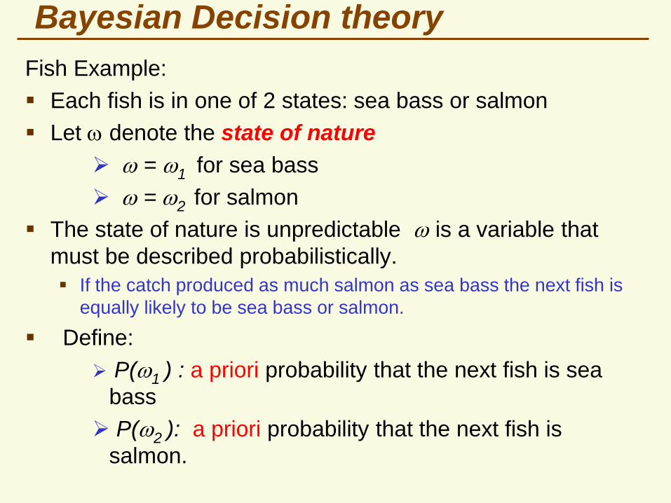
Fish Example:
Each fish is in one of 2 states: sea bass or salmon
Let w denote the state of nature
w = w1 for sea bass
w = w2 for salmon
The state of nature is unpredictable w is a variable that
must be described probabilistically.
If the catch produced as much salmon as sea bass the next fish is
equally likely to be sea bass or salmon.
Define:
P(w1 ) : a priori probability that the next fish is sea
bass
P(w2 ): a priori probability that the next fish is
salmon.

4
Bayesian Decision theory
If other types of fish are irrelevant:
P( w1 ) + P( w2 ) = 1.
Prior probabilities reflect our prior knowledge
(e.g. time of year, fishing area, …)
Simple decision Rule:Make a decision without seeing the fish.
Decide w1 if P( w1 ) > P( w2 ); w2 otherwise.
OK if deciding for one fish
If several fish, all assigned to same class
In general, we have some features and
more information.

Cats and Dogs
Suppose we have these conditional probability
mass functions for cats and dogs
P(small ears | dog) = 0.1, P(large ears | dog) = 0.9
P(small ears | cat) = 0.8, P(large ears | cat) = 0.2
Observe an animal with large ears
Dog or a cat?
Makes sense to say dog because probability of
observing large ears in a dog is much larger than
probability of observing large ears in a cat
P[large ears | dog] = 0.9 > 0.2= P[large ears | cat] = 0.2
We choose the event of larger probability, i.e.
maximum likelihood event
6
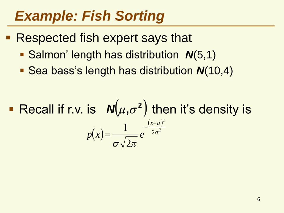
Example: Fish Sorting
Respected fish expert says that
Salmon’ length has distribution N(5,1)
Sea bass’s length has distribution N(10,4)
Recall if r.v. is then it’s density is
2
2
2
2
1
x
exp
2,N

7
Class Conditional Densities
2
52
2
1|
l
esalmonlp
4*2
102
22
1|
l
ebasslpfixed fixed

8
Likelihood function
Fix length, let fish class vary. Then we get
likelihood function (it is not density and not
probability mass)
bassclassife
salmonclassife
classlpl
l
8
10
2
5
2
2
22
1
2
1
|
fixed

9
Likelihood vs. Class Conditional Density
length7
Suppose a fish has length 7. How do we classify it?
p(l | class)

ML (maximum likelihood) Classifier
2
52
2
1|
l
esalmonlp
4*2
102
22
1|
l
ebasslp
Instead, we choose class which maximizes likelihood
We would like to choose salmon if
basslengthsalmonlength |7Pr|7Pr
However, since length is a continuous r.v.,
0|7Pr|7Pr basslengthsalmonlength
ML classifier: for an observed l:
basslpsalmonlp |?|
salmon
bassin words: if p(l | salmon) > p(l | bass),
classify as salmon, else classify as bass

11
7
p( 7 |bass)
p( 7 |salmon)
Thus we choose
the class (bass)
which is more
likely to have given
the observation
ML (maximum likelihood) Classifier
12
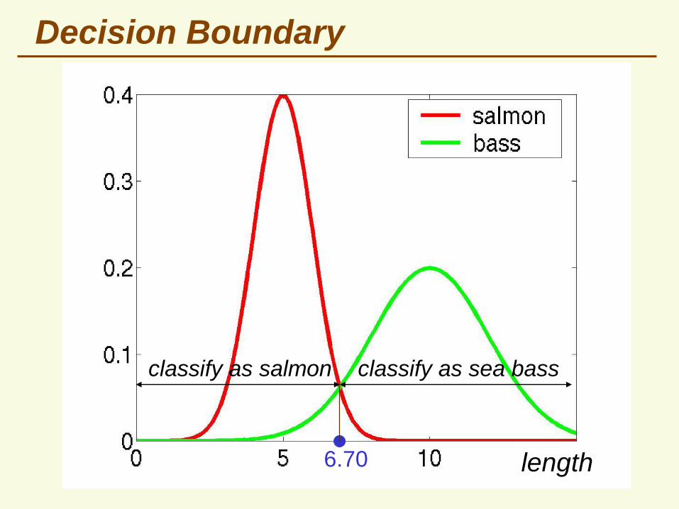
classify as salmon classify as sea bass
Decision Boundary
length6.70
13
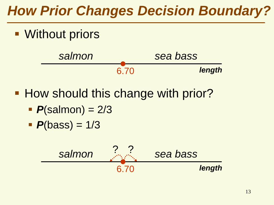
How Prior Changes Decision Boundary?
Without priors
How should this change with prior?
P(salmon) = 2/3
P(bass) = 1/3
6.70
salmon sea bass
? ?
length
6.70
salmon sea bass
length
14
Bayes Decision Rule
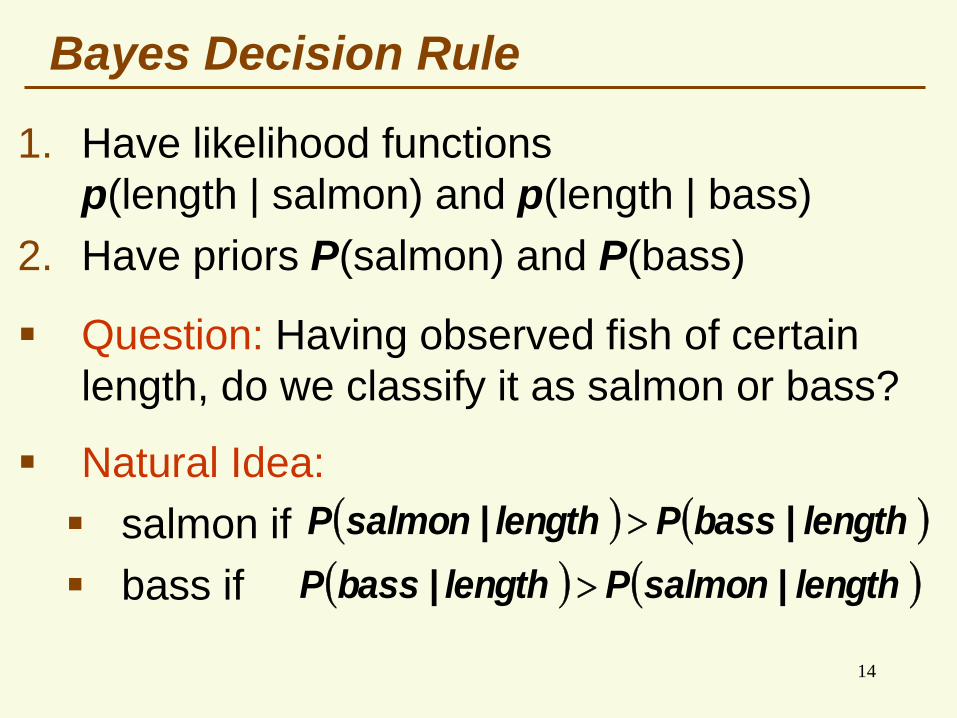
1. Have likelihood functions
p(length | salmon) and p(length | bass)
2. Have priors P(salmon) and P(bass)
Question: Having observed fish of certain
length, do we classify it as salmon or bass?
Natural Idea:
salmon if
bass if
length|bassPlength|salmonP
length|salmonPlength|bassP

15
Posterior
P(salmon | length) and P(bass | length)
are called posterior distributions, because
the data (length) was revealed (post data)
How to compute posteriors? Not obvious
From Bayes rule:
lengthp
salm onPsalm onlengthplengthP(salm on
|| )
lengthp
bassPbass|lengthplength|bassP
Similarly:

16
MAP (maximum a posteriori) classifier
lengthp
bassPbass|lengthp?
lengthp
salmonPsalmon|lengthp
salmon
bass
bassPbass|lengthp?salmonPsalmon|lengthp
salmon
bass
lengthbassPlengthsalmonP |?|
bass
salmon
17
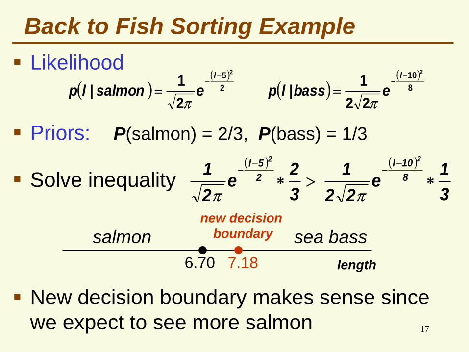
Back to Fish Sorting Example
2
52
2
1|
l
esalmonlp
8
102
22
1|
l
ebasslp
Likelihood
Priors: P(salmon) = 2/3, P(bass) = 1/3
3
1e
22
1
3
2e
2
18
10l
2
5l22
Solve inequality
6.70
salmon sea bass
length7.18
new decision
boundary
New decision boundary makes sense since
we expect to see more salmon

Prior P(s)=2/3 and P(b)= 1/3 vs.
Prior P(s)=0.999 and P(b)= 0.001
7.1 8.9 length
salmon
bass

Likelihood vs Posteriors
length
P(salmon|l) P(bass|l)
p(l|salmon)
p(l|bass)
likelihood
p(l|fish class)
density with
respect to
length, area
under the
curve is 1
posterior P(fish class| l)
mass function with respect to fish class, so for
each l, P(salmon| l )+P(bass| l ) = 1

More on Posterior
lP
cPc|lPl|cP
Prior
(given)posterior density
(our goal)
likelihood
(given)
normalizing factor, often do not even need
it for classification since P(l) does not
depend on class c. If we do need it, from
the law of total probability:
Notice this formula consists of likelihoods
and priors, which are given
basspbass|lpsalmonpsalmon|lplP

21
More on Priors
Prior comes from prior knowledge, no data
has been seen yet
If there is a reliable source prior knowledge,
it should be used Some problems cannot even be solved
reliably without a good prior

More on Map Classifier
lP
cPc|lPl|cP
posteriorlikelihood prior
If P(salmon)=P(bass) (uniform prior) MAP classifier
becomes ML classifier c|lPl|cP
cPc|lPl|cP
Do not care about P(l) when maximizing P(c|l )
proportional
If for some observation l, P(l|salmon)=P(l|bass), then
this observation is uninformative and decision is
based solely on the prior cPl|cP

23
Justification for MAP Classifier
Let’s compute probability of error for the
MAP estimate:
l|bassP?l|salmonP
bass
salmon
For any particular l, probability of error
Pr[error| l ]=if we decide salmonP(bass|l)
if we decide bassP(salmon|l)
Thus MAP classifier is optimal for each
individual l !

Justification for MAP Classifier
We are interested to minimize error not just for
one l, we really want to minimize the average
error over all l
dllpl|errorPrdll,errorperrorPr
If Pr[error| l ]is as small as possible, the integral is
small as possible
Thus MAP classifier minimizes the probability of error!
But Bayes rule makes Pr[error| l ] as small as
possible

More General Case
Have more than one feature d21 x,...,x,xx
m21 c,...,c,c Have more than 2 classes
Let’s generalize a little bit

26
More General Case
As before, for each j we have
is likelihood of observation x given that
the true class is
is prior probability of class
is posterior probability of class given
that we observed data x
jcPjc
jc|xp
jc
x|cP j jc
Evidence, or probability density for data
m
1j
jj cPc|xpxp
need to make this
as small as possible
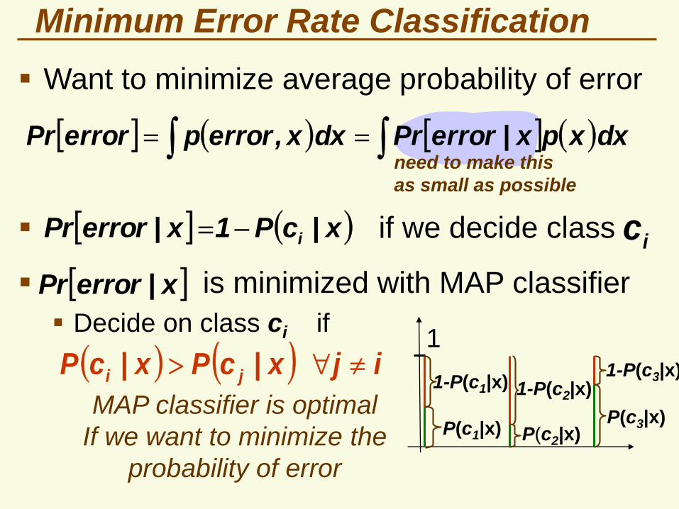
Minimum Error Rate Classification
Want to minimize average probability of error
dxxpx|errorPrdxx,errorperrorPr
x|cP1x|errorPr iic if we decide class
x|errorPr is minimized with MAP classifier
Decide on class ci if
ijx|cPx|cP ji
MAP classifier is optimal
If we want to minimize the
probability of error
1
P(c1|x) P(c2|x)P(c3|x)
1-P(c1|x) 1-P(c2|x)1-P(c3|x)

28
General Bayesian Decision Theory
Suppose some mistakes are more costly than others (classifying a benign tumor as cancer is not as bad as classifying cancer as benign tumor)
k21 ,...,,
In some cases we may want to refuse to
make a decision (let human expert handle tough case)
allow actions
Allow loss functions describing loss
occurred when taking action when the true
class is
ji c|
i
jc

Conditional Risk
Suppose we observe x and wish to take
action i
If the true class is , by definition, we incur
loss ji c|jc
Probability that the true class is after
observing x is jc
x|cP j
m
1j
jjii x|cPc|x|R
The expected loss associated with taking
action is called conditional risk and it is:i

Conditional Risk
m
1j
jjii x|cPc|x|R
sum over disjoint events
(different classes)
probability of
class given
observation xjc
penalty for
taking action
if observe xi
jc
part of overall penalty
which comes from event
that true class is
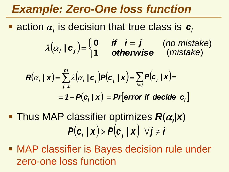
Example: Zero-One loss function
action is decision that true class is
m
1j
jjii x|cPc|x|R
x|cP1 i
MAP classifier is Bayes decision rule under
zero-one loss function
otherwise
jiifc ji 1
0|
(no mistake)(mistake)
ji
j x|cP
Thus MAP classifier optimizes R(i|x)
ijx|cPx|cP ji
ici
icdecideiferrorPr

Overall Risk
Decision rule is a
function (x) which for
every x specifies action
out of k21 ,...,,
need to make this as small as possible
dxxpx|xRR
The average risk for (x)
Bayes decision rule (x) for every x is the action
which minimizes the conditional risk
m
1j
jjii x|cPc|x|R
Bayes decision rule (x) is optimal, i.e. gives the
minimum possible overall risk R*
X
k21 ,...,, x1
x2
x3
(x1)
(x2)
(x3)

Bayes Risk: Example
Salmon is more tasty and expensive than sea bass
2
52
2
1|
l
esalmonlp
4*2
102
22
1|
l
ebasslp
Likelihoods
2bass|salmonsb classify bass as salmon
1salmon|bassbs classify salmon as bass
0bbss no mistake, no loss
l|bPl|bPl|sPl|salmonR sbsbss
Priors P(salmon)= P(bass)
l|sPl|bPl|sPl|bassR bsbbbs
Risk
m
1j
jj x|cPc|x|R l|bPl|sP bs

Bayes Risk: Example
l|bPl|salmonR sb l|sPl|bassR bs
Bayes decision rule (optimal for our loss function)
l|sP?l|bP bssb
salmon
bass
Need to solve sb
bs
l|sP
l|bP
sb
bs
s|lP
b|lP
sPs|lPlp
lpbPb|lP
Or, equivalently, since priors are equal:

Bayes Risk: Example sb
bs
s|lP
b|lP
Need to solve
1
exp221
exp22
2
5l
8
10l
2
2
Substituting likelihoods and losses
1
exp
exp
2
5l
8
10l
2
2
1ln
exp
expln
2
5l
8
10l
2
2
0
2
5l
8
10l22
0l20l3 2 6.6667l0
6.67
salmon sea bass
length6.70
new decision
boundary

36
fixed number
Independent of xlikelihood
ratio
Likelihood Ratio Rule
In 2 category case, use likelihood ratio rule
1
2
1121
2212
2
1
cP
cP
c|xP
c|xP
If above inequality holds, decide c1
Otherwise decide c2

Discriminant Functions
All decision rules have the same structure:
at observation x choose class s.t.
ijxgxg ji
ic
ML decision rule: ii c|xPxg
MAP decision rule: x|cPxg ii
Bayes decision rule: x|cRxg ii
discriminant
function

38
Decision Regions
Discriminant functions split the feature
vector space X into decision regions
i2 gmaxxg
1c
3c1c
2c
3c
39
Important Points
If we know probability distributions for the
classes, we can design the optimal
classifier
Definition of “optimal” depends on the
chosen loss function
Under the minimum error rate (zero-one loss
function
No prior: ML classifier is optimal
Have prior: MAP classifier is optimal
More general loss function
General Bayes classifier is optimal
Recommended