Revisiting the Dynamic Effects of Oil Price Shockson Small Developing Economies

Imran H. Shah, Carlos Diaz Vela, Yuan WangNo. 65 /17

BATH ECONOMICS RESEARCH PAPERS

Department of Economics

Revisiting the Dynamic Effects of Oil Price Shocks on Small Developing Economies

17 March 2017

1. Imran H. Shah (First and corresponding author), Department of Economics,

University of Bath, BA2 OJH, United Kingdom. Email: i.h.shah@bath.ac.uk,

imran_gillani664@hotmail.com. Phone: +447825166631

2. Carlos Diaz Vela (Co-Author), University of Leicester, UK.

3. Yuan Wang (Co-Author), University of Southampton, UK.

ABSTRACT

This paper examines the dynamic effects of oil price, aggregate demand and aggregate supply shocks on output and inflation in four small developing economies using a structural VAR model. For all countries, despite finding the expected response of output to oil price shocks, an upward causal effect of oil price innovations on the domestic price level is established which adversely accompanies the growth stimulating effects in oil-exporting countries. This paper also finds asymmetric effects of oil price changes on macroeconomic variables in all sample countries. Finally, our empirical results find two further things: firstly, that for Malaysia, Pakistan and Thailand, nominal demand and supply shocks are the main sources of fluctuations in inflation and output respectively, whereas for Indonesia the converse holds and secondly that whilst the 1998 recession was largely induced by only supply and demand shocks the recession of 2008-09 could potentially be explained by oil price changes.

Key words: Macroeconomic fluctuations, Oil price, Structural VAR models, Asian developing economies

JEL Classification Numbers: C32, E31, E32, F41, O40, O53

2

1. INTRODUCTION

In the existing literature, the relationship between changes of oil price (OP) and

macroeconomic fluctuations has been intensively discussed (e.g., Abeysinghe, 2001;

Bjornland, 2000; Hamilton, 1983, 1996, 2003, 2009 and 2011; Kilian, 2008 and 2009; Kilian

and Vigfusson, 2013; Mork, 1989). A large amount of empirical evidence supports the

existence of a causal relationship from OP changes to output fluctuations (Cunado and Perez

de Gracia, 2003; Jimenez-Rodriguez and Sanchez, 2005) and also in the variations of

domestic aggregate price level (Barsky and Kilian, 2004; Elder and Serletis, 2010;

Rotemberg and Woodford, 1996). The seminal contribution in this area is credited to

Hamilton (1983), the empirical work shows that the OP shocks contribute to some recessions

in the US before 1972, but not necessarily lead a recession. In alignment with the previous

finding, Hamilton (1996) claims a non-linear relationship between OP and output. More

precisely, OP increases (whether the OP has exceeded the maximum OP in recent years) are

believed to be more important than OP decreases in predicting output growth, as suggested

by Hamilton. Elder and Serletis (2010) find that the volatility of the OP has statistically

significant negative effects on output: exacerbates the negative impact to a negative OP shock

and dampens the impact to a positive OP shock. The recent work of Kilian and Vigfusson

(2013) states that the OP is not helpful for out-of-sample forecasting in the asymmetry

nonlinear models, but useful in symmetric nonlinear models. It is possible to forecast the

2008-09 recession by using the latter.

Conventional wisdom suggests that the correlation between OP shocks and

macroeconomic fluctuations comes from a set of fundamental shocks, which hit all sectors of

the economy. A large number of studies has focused on identifying the source of that shocks.

The seminal ideas come from Hamilton (1983) and Kilian (2009), who focus on the demand

and supply side respectively. Both authors provide extraordinary explanations and rigorous

proofs. Hamilton believes that oil supply shocks, usually caused by a shortfall of OPEC oil

production due to political events in the Middle East, has a major role in explaining the

dynamics of OP and real GDP movements. However, Kilian (2009) believes that oil demand

and speculative OP shocks linked with global economic activity have being the major driving

force of oil price fluctuations since 1973.

The variations of OP are expected to have very different effects on oil-importing and

oil-exporting countries. Brown et al. (2004) show that increased OP has a similar effect to a

tax, which is collected by oil-exporting countries from oil-importing countries. Most of the

3

empirical studies mainly related to developed economies have confirmed that OP changes

have a negative effect on output growth in oil-importing countries (e.g., Jimenez-Rodriguez

and Sanchez, 2005; Schneider, 2004; Schubert and Turnovsky, 2011). Increases in OP and

the resultant instability affect the economy through higher input costs, reallocation of

resources, decreases in income and depreciation of currency. As a result, economic

performance is depressed while inflation and unemployment are raised. A sudden increase in

the OP causes an exogenous inflationary shock as high OP puts pressure on the general price

level, and leads to higher interest rates. The former is very likely lead to a recession. Other

studies (e.g., Bjornland, 2000) indicate that an increase in OP is associated with higher

growth in net oil-exporting countries through increased state revenue, which leads to higher

national income and currency appreciation. Bjornland (2009) states that high OP also affects

oil-producing countries through negative trade effects by rising inflation and since oil-

importing countries suffer from oil induced recession and therefore demand fewer exports

from oil-exporting countries. For those oil-exporting countries with a large export sector, the

negative trade effect may indeed off-set the positive wealth effect, which leaves the net effect

ambiguous.

The recent experience in Asian countries somehow forms the hypothesis of non-

negligible effects of OP shocks on economic fluctuation under some circumstances. Cunado

and Perez de Gracia (2005) investigate potential impacts of OP on economic activity and

consumer price indexes for six Asian countries and they find that results are sensitive to the

choice of the OP (domestic or international). The short-run effects of OP on economic growth

and inflation are statistically significant. Spikes in OPs prior to the global crisis led to high

inflation rates in most South and South East Asian countries evidenced by double-digit

figures. The inflationary pressures also induced large budget deficits and balance of payment

concerns. Lescaroux and Mignon (2009) and Tang et. al. (2010) both find negative effects of

OP on macroeconomic variables in China. However, in the recent work of Schubert and

Turnovsky (2011), the evidence shows that recent OP shocks have a tempered effect on

economic activity on developing countries compared with those in 1970s and 1980s.1 One

obvious explanation would be the fall in both proportion and influence of oil in the economy

due to more credible policy response, more flexible labour market and appearance of oil

substitutes.

1 See Blanchard and Gali (2008) for a detailed review.

4

Mork (1989), Lee et al. (1995) and Hamilton (1996) introduced asymmetric

specifications of the OP to reconstruct the relationship between OP and economic

performance. It has been asserted in the literature that the relationship between OP shocks

and macroeconomic variables is non-linear and many studies have suggested the possibility

of an asymmetric impact of OP shocks on macroeconomic variables (Mork, 1989; Lee and

Ni, 2002; Jimenez-Rodriguez and Sanchez, 2005; Hamilton, 2009 and 2011; An et al., 2014,

Kilian and Vigfusson, 2011). According to these studies, the negative effects of higher OPs

are greater than the positive effects of lower OPs in oil-importing countries. On the other

hand, Moshiri (2015) examines the asymmetric effect of OP shocks on macroeconomic

performance in the nine major oil-exporting countries using a VAR model. He finds that the

negative OP shocks have damaging impacts on output of oil-exporting countries, however

positive OP shocks do not stimulate output.

The main contribution of this paper is to extend the existing empirical literature in two

directions. Firstly, we investigate the linear effects of OP shocks, in addition to nominal AD

and AS shocks, on output and inflation in four Asian developing countries: Indonesia,

Malaysia, Pakistan and Thailand. The reason behind our investigation of these countries is

that there is little previous evidence on the effects. Secondly, we investigate the asymmetric

effects of OP by using a non-linear method, namely the asymmetric specification. The

conjecture is that positive oil price shocks could have larger effects on growth and that

negative oil price shocks do not substantially affect growth for oil-importing countries (and

vice versa for oil-exporters). The study uses a structural VAR approach, which imposes both

short-run and long-run restrictions to identify different structural shocks and to carry out both

linear and non-linear models.

Indonesia is the largest oil producer in Southeast Asia and is also a major oil-exporter

during the period analysed due to its considerable oil reserves. According to the World Bank,

Indonesian exports account for about 40% of GDP. Malaysia has the third highest oil reserves

of the Southeast Asian countries but its net oil-exports are very small due to the small gap

between domestic production and demand. Thailand produces some oil domestically,

however it is still a significant oil-importing country due to the large domestic demand of oil.

In Thailand, two thirds of oil demand is imported from abroad, which accounts for a large

proportion of GDP. Pakistan is also an oil-importing country since it has limited domestic oil

reserves and relies heavily on imports. However, Pakistan demands the smallest amount of

oil among the four sample economies. Oil-importing developing economies are generally

5

considered highly vulnerable to external shocks, and prominent among these is volatility in

the OP because an OP increase transfers income from countries with a higher propensity to

consume to countries with lower propensity to consume. Given the above facts about

production and demand, this study will consider Indonesia and Malaysia as oil-exporting

countries, and Pakistan and Thailand as oil-importing countries.

Although Indonesia and Malaysia are net oil-exporters, due to the exhaustion of oil

fields and the lack of investment in exploration of oil, the economy experienced stagnant oil

production. Consequently, the oil market is relatively tight due to the small gap between

domestic production and oil demand. It is interesting to investigate the impact of the OP on

countries which are in the process of transforming themselves from net-exporters to net-

importers. For all sample countries, governments provide subsidies on the OP in order to

reduce the adverse effect of OP shocks on real economic activities. Consequently, when the

international OP rose from 50 dollars per barrel in 2007 to 140 dollars per barrel in 2008 a

significant budget deficit was induced. According to the World Bank (2013)2, the ratios of

government budget deficit to GDP increased from -0.08% to -1.6% in Indonesia, -4.6% to -

6.7% in Malaysia, -3.9% to -7.2% in Pakistan and -1.3% to -4.8% in Thailand after the 2008

recession. In the past three decades, these countries have experienced an increased demand

for energy, particularly for oil following the deepening of economic development. There has

recently been a period of negative growth which was dominated by the global financial crisis

and also with the adverse effect of an OP shock. Identifying and understanding the effects of

various shocks on macroeconomic fluctuations in the sample countries, particularly the

effects of OP shocks, could provide some policy recommendations for regional co-operation

in the Asian-Pacific area. This could help to minimize negative influences from global

economic fluctuations and achieve macroeconomic stability for sustainable growth and

development.

The rest of the paper is organised as follows. Section 2 introduces a theoretical model

with separated OP shocks in addition to AD and AS shocks. The empirical methodology and

estimation results are reported in Section 3. Finally, a few concluding remarks are provided in

Section 4.

2. THEORETICAL MODEL

2 http://siteresources.worldbank.org/DEC/Resources/84797-1154354760266/2807421-1382041458393/9369443-1382041470701/Oil_Price_Volatility.pdf

6

The theoretical framework in this paper is a modified AD and AS model. The effects of

different structural shocks on macroeconomic variables have been modelled explicitly.

The Lucas supply curve (Lucas, 1972 and 1973) with rational expectations can be defined as:

(1)

where AS , is a function of natural rate of output and the difference between actual

domestic price level and its expectation given all available past information . Taking

the expectation conditional on time t-1 and rearranging Eq. (1) gives:

(2)

where represents productivity shock, which can be further decomposed into a supply (defined as domestic supply) shock and an OP shock (see Bjornland, 2000).

(3)

Eq. (3) describes the AS curve where output increases as a result of an unpredicted increase

in price levels, an OP shock and a positive realization of the AS shock . High OPs are

considered as technology shocks, which reduce output level through increasing production

cost in oil-importing countries. In another words, the oil price affects the supply side of the

economy by increasing the cost of inputs and necessitating a rearrangement of resources, thus

leading to lower GDP.3 Oil price hikes may add to inflationary pressures and reduce real

incomes and, as a result, consumer expenditure will be compressed. Furthermore, real output

may also be affected in the face of weaker domestic demand and reduced company's

profitability. Research’s finds that OP affects output and price levels, and the lower level of

demand can be counteracted through the corresponding monetary policies implemented by

the central banks (Hamilton, 1996, Hamilton, 2003 and Hooker, 2002). High OPs affect the

economy of oil-importing countries through increased marginal costs and inflation. It is

therefore expected that for oil-importing countries. In contrast, oil-exporting countries

will respond to the same shock positively ( ) due to an increase in national income

3 Brown et al. (2004) argues that rising OPs decrease purchasing power and consumer demand in oil-importing economies, and that the opposite should be expected for oil-exporting nations.

1 1[ ( | )]st t t t t ty y p E p

sty ty

tp 1t

1 1 1 1( | ) [ ( | )]st t t t t t t t ty E y p E p

t

1 1 1 1( | ) [ ( | )]s s opt t t t t t t t t ty E y p E p

opt

st

0

0

7

through greater oil export revenue. This is especially applicable to those oil-exporting

countries where the oil sector is large compared with the rest of the economy.

The demand curve can be expressed as:

(4)

where AD, , is a function of literal money , domestic price level and oil price .

Similarly as for the supply side, taking expectations conditional on time and rearranging

Eq. (4) gives,

(5)

Eq. (5) explains that AD equals its expected value given the information available at the

end of period t-1, plus the effect of an OP shock and nominal demand (defined as a price

shock) shock . Oil price fluctuations can also affect the economy through the demand side

via the income effect. Spikes in the OP will shift income from oil-importing countries to net

oil-exporting countries. Therefore, in each category we would expect gamma γ to be less

than 0 and greater than 0 respectively.

The economy is in equilibrium when,

(6)

Hence we have,

(7)

(8)

Following Bjornland (2000), we assume that world OP can only be affected by shocks

to oil demand and oil supply, while other factors (such as political events) are considered as

exogenous to the OP.4 Hence,

4 In particularly, our sample countries are small economies. Hence, this is a reasonable assumption.

dt t t ty m p op

dty tm tp top

1t

1 1 1 1( | ) [ ( | )]d d opt t t t t t t t t ty E y p E p

opt

dt

s dt t ty y y

1 11 1( | )

1 1 1s d op

t t t t t t tp E p

1 11( | )

1 1 1s d op

t t t t t t ty E y

8

(9)

The early studies included Blanchard and Gali, 2010; Bjornland, 2000; Hamilton, 1983,

2003; Jimenez-Rodriguez and Sanchez, 2005; Schmitz el al, 2007; Tang, 2010 who regard

OP changes are as exogenous to the contemporaneous value of macroeconomic variables.

Furthermore, they prove that oil shocks affect macroeconomic variables whereas changes in

these variables cannot affect OP which is exogenously determined by the world’s demand

and supply shocks. The reason behind this is that OP has been dominated by political events

like the OPEC embargo in 1973, the Iranian revaluation in 1978-1979, the Iran-Iraq War in

1980-81, the Gulf War in 1990-1991, and increasing demand confronting declining world

production in 2003-2008.

Eqs. (7) - (9) give us the structural form model in the paper. Each structural shock (OP

shock, , AD shock, and AS shock, ) is a white noise and they are assumed to be

uncorrelated with each other. In the short run, OP, AS and AD shocks affect the output level

due to nominal and real inflexibilities as exhibited in Eq. (8). In alignment with Blanchard

and Quah (1989), we assume AS shocks have permanent effect on output level, while AD

shocks only affect output level in the short run. The OP shocks are assumed to be exogenous,

which is consistent with the recently work of Kilian and Vigfusson (2013).

3. EMPIRICAL METHODOLOGY AND RESULTS

3.1 Data Description

In this section we investigate the response of different types of shocks into four Asian

countries. The data used in this study is real OP, real GDP and consumer price index (CPI)

for 4 sample economies: Indonesia, Malaysia, Pakistan5 and Thailand.6 For all countries,

5 For Pakistan, quarterly data series for GDP are not publish or are not available for a longer period of time. The industrial production index is used as a proxy of the real GDP. The quarterly series for the industrial production is downloaded from IMF, IFS, 2015. Although, industrial production data for Pakistan is available before 1990 but in order to be consistent with other countries we consider it from 1990. 6 Data are downloaded from the International Monetary Fund (IMF), International Financial Statistics (IFS), Edition: July 2015. The real GDP series are based on authors’ calculation from the GROSS DOMESTIC PRODUCT (GDP) (Units: National Currency; Scale: Billions) and GDP DEFLATOR (2005=100) for two countries except Indonesia, where the consumers’ price index, CPI, has been used as the deflator. . The domestic nominal OP series is calculated from PETROLEUM AVERAGE CRUDE PRICE (Units: US Dollars per Barrel) converted to each country’s national currency. For Malaysia and Thailand, the real OP is computed from deflated by implicit consumer price index, while for Indonesia and Pakistan, where the CPI has been used as the

1w w opt t top op

opt

dt

st

9

quarterly GDP data is not available for an extended period of time and therefore, the sample

starts at the earliest available date. The time-spans differ across countries depending on the

availability of data: Indonesia (1990q1 to 2015q4), Malaysia (1991q1-2015q4), Pakistan

(1990q1-2015q4) and Thailand (1993q1-2015q4). The data are transformed by taking

logarithms.

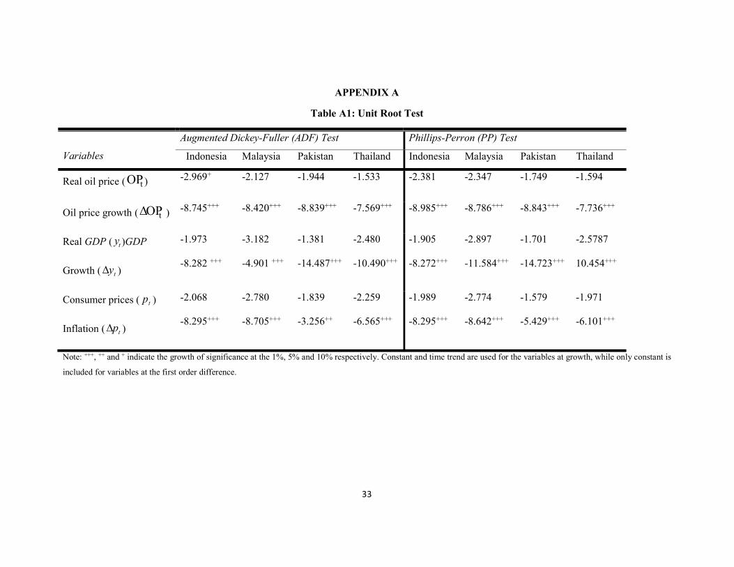
3.2 Empirical Model and Estimation Results As shown in Appendix A, Table A1, the unit root tests (both Augmented Dickey Fuller

and Phillips Perron tests) indicate that none of these three series are stationary, so that all of

them are differenced before estimation. Before proceeding further, a few pre-estimation tests

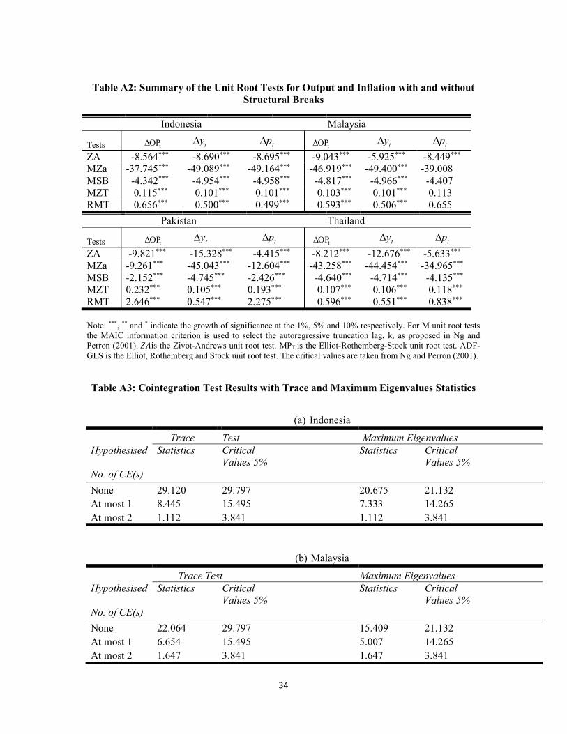
are conducted. As exhibited in Appendix A, Table A2, we use the approach introduced by

Zivot and Andrews (1992) to test the null of unit root against structural break-stationary

alternative hypothesis. Furthermore, we test the OP growth, inflation and GDP growth data

with several unit root tests with structural breaks in essentially trend-stationary series,

namely, ERS-PT Elliott-Rothenberg-Stock, NP-MZα Ng-Perron, SKP-MSB Silvestre-Kim-

Perron, SKP-MZT Silvestre-Kim-Perron and PP- Zα Phillips-Perron7.The results indicate

that all of these three series are stationary at first difference for each country (see Appendix

A, Table A2). The results are consistent with the conventional unit root test without structural

breaks. For all countries, the break period for each series is reported in table Appendix A,

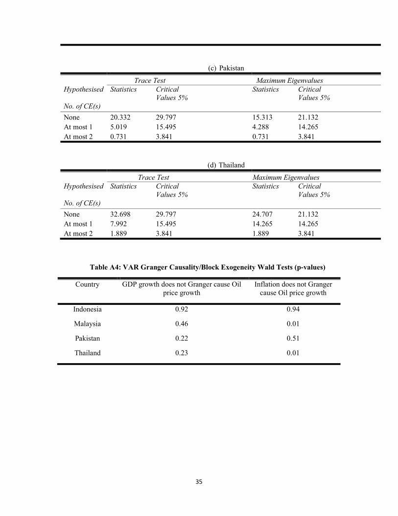
Table A2. The Johansen test of cointegration is performed next to the level series with

appropriate assumptions on trends and lags to check whether the variables are cointegrated in

each country (see Appendix Table A3). Generally speaking, there is no cointegration

evidence among three series in any country.8

Notice, then, that we are modelling the rate of growth of GPD and OP as well as

inflation. A reduced-form VAR (k) model is fitted to the stationary data where the a priori

assumption of weakly exogenous OP is imposed. Therefore, denoting the lower case names

of the variables as the log-transformed values of oil prices (op), GDP (y) and CPI (p), the

model used for estimation is

deflator. The CPI series are given as follows: CPI:17 CAPITAL CITIES (Indonesia), CPI PENINSULAR MALAYSIA (Malaysia), CPI:12MAJOR CITIES ALL INC. (Pakistan), CPI: URBAN (Thailand). 7 Ng-Perron (2001) proposed four test statistics that are based upon the GLS-detrended data. 8 Both the trace and maximum eigenvalues test statistics indicate no cointegration at the 0.05 level for Indonesia, Malaysia and Pakistan, while at the 0.01 level for Thailand.

10

(10)

where (j=1,2,3) is a vector containing deterministic variables used to model variable j.

This vector contains a constant that accounts for the possibility of the presence of a

deterministic time trend in the growth of the variables and a set of intervention variables to

account for the structural breaks suggested by the stationarity tests commented above9. More

detailed information regarding the estimation results can be obtained from the authors on

request. The exogeneity property of OP growth is manifested in the first equation of system

(10) as GDP growth and inflation do not affect OP, which is driven only by its past dynamic.

To validate the exogeneity assumption of the OP, we perform a Granger causality test to

examine whether the lagged values of growth and inflation have explanatory power on OP

growth and the results are reported in Appendix A4. The results show that OP is not affected

by real GDP for all countries. The finding is consistent with previous studies such as

Bjornland (2000) and Tang (2010). Furthermore, inflation does not Granger cause OP for

Indonesia and Pakistan but for Malaysia and Thailand the exogeneity condition for OP is

valid only at 1% level of significance.

The model can be written in compact form as

∆ = + ∑ ∆ + , (11)

where = (, , )′ and = , , ~(, ), where is a positive definite

matrix containing the variance and covariances of the errors of the reduced form model.

Estimation of this model is performed using the JMulTi software10 and EViews. Summarized

estimation results are shown in Table 111. The first two rows indicate the number of effective

observations used in estimation and the autoregressive order used in each model. For all

countries the optimal lag selected by the Bayesian Information Criteria indicates a large value

of 2. The next two rows indicates the value of the multivariate Box-Pierce portmanteau test

9 The results are not reported but up to request. 10 Free software available for download at http://www.jmulti.de/, accompanying Lüktepohl (2006). 11 Estimation has been performed also using annual data for Pakistan and results seem to be robust.

1 1 111

2 2 21 22 231 1 1

3 3 31 32 331 1 1

'

'

'

kop

t t j t j tj

k k ks

t t j t j j t j j t j tj j j

k k kd

t t j t j j t j j t j tj j j

op a a op e

y a a op a y a p e

p a a op a y a p e

x

x

x

opte

ste

dte

11

for autocorrelation along with the corresponding p-values, indicating that there is no

significant correlation left in each model.

[TABLE 1]

Table 1: Model Estimation Results

N

Indonesia Malaysia Pakistan Thailand

104 100 104 92

K 2 2 2 2

Q 152.02 126.09 115.51 151.57

p-val (Q) 0.09 0.58 0.91 0.10

M-JB 216.30 376.01 19.02 20.96

p-val (JB) 0.00 0.00 0.00 0.00

0.52 0.58 0.59 0.51

||Llik

2.40e-9

544.12

5.65e-11

693.83

2.58e-09

551.82

1.26e-10

599.68

Next, the multivariate Jarque-Bera test indicates departure from the assumption of

normality of the residuals. However, given the good fit of the model, and that there are not

significant outliers left unmodelled, we consider the estimates satisfactory. The maximum

eigenvalue of the autoregressive polynomial () indicates no problem of persistence or

cointegration as tested initially using Johansen’s cointegration tests (see Appendix B).

Finally, the value of the likelihood function, the determinant of the covariance matrix and the

Akaike and Bayesian Information Criteria are also reported. Estimates have been checked for

robustness indicating stability of the estimates.

The impulse-response analysis is performed using the Wold decomposition as

∆ = + + ∑ , (12)

where ( ⋯ ) = + ∑ and L the lag operator. The convergence

of the multivariate polynomial is assured in the studied cases by the stability of the estimated

VAR models. Notice that the elements of the vector of errors are contemporaneously

12

correlated so that a shock in one variable ( ≠ 0) implies an instantaneous shock in the rest

of variables. To avoid this problem and obtain isolated shocks on each variable, an

orthogonalization of it is needed in order to obtain the impulse responses. This model is

denoted as the Structural VAR(k) model and its (structural) shocks = ( , , )′contemporaneously uncorrelated. Here we denote

the structural shock of OP, is

interpreted as an AS shock and as AD shock. The identification of the structural VAR

model (or the orthogonalization of the reduced form errors) can be achieved in various ways;

here we follow the Blanchard and Quah (1989) method which consists of setting a set of

restrictions on the matrix of long run effects as

= (1) =

(13)

According to the theoretical model in Eq. (9), real OP are free from domestic demand

and supply shocks, i.e., the contemporaneous effects of AS and AD shocks on OP are zero.

Therefore, we have 2 more restrictions: zero short-run restrictions on OP, = = 0.

Finally, we impose a long-run restriction (Blanchard and Quah, 1989), where AD shocks

have no long-run effects on the growth of output, = 0 . For simplicity the structural

shocks are normalized to have unit variance so that, denoting ∗ the restricted matrix,

then () = ∗ ∗.

To account for asymmetric effects, this study separates OP innovations into positive

and negative parts following Mork (1989)12. Mork (1989) introduces an asymmetric concept

of OPs and proposes to separate positive from negative OP changes. He indicated that there is

an asymmetry effect of OPs on macroeconomic variables. He confirmed that positive OP

shocks have a significantly negative impact on GDP while negative OP shocks have no

significant effects for oil-importing countries. He defines positive and negative quarterly OP

( tOPΔ and

tOPΔ respectively) changes in the following ways;

1ttt OPOP,0maxOPΔ (14)

1ttt OPOP,0minOPΔ (15)

12 The approaches of Hamilton (1996) and Lee et al. (1995) are not used due to the current size of the paper and also due to the facts that the results used by Mork’s approach are more explanatory.

opt

st

dt

13

3.3 Impulse Response Analysis: Linear Specification

The accumulated response of each variable to a shock of magnitude equal to two

standard deviation confidence interval (dashed line) is plotted in Figures 1 to 6. Generally

speaking, OP shocks seem to have some long-run effects on the output growth in the four

sample economies, but the magnitudes are not comparable with the AS shocks. The OP

shocks have, as expected, a positive effect on the growth of output and inflation in Indonesia

and Malaysia, although the effect is insignificant as growth is raised by only 0.5% and 0.8%

after the shock for Indonesia and Malaysia respectively ,13 see figure 1a-1b14. This positive

output response is consistent with the conventional wisdom that an increase in OPs leads to a

rise in the revenue and income of oil-exporting countries (see Ito (2008), Bjornland (2000)

and Rautava (2004). However, the confidence interval confirms that after the first quarter OP

shocks have a negligible effect on output in the long-run. This may be because Indonesia

recently experienced an increase in the production dependency on oil and has a high share of

oil in the consumption bundle. In addition, the Indonesian economy has experienced stagnant

oil production when compared to demand due to the exhaustion of old oil fields and lack of

investment in exploration for oil reserves. Hence, an increasing OP may have a negligible

positive effect on its output.

[FIGURE 1]

Figure 1: Accumulated Effects of OP Shocks on GDP Growth

13 This result contradicts that of Salim and Rafiq (2011) findings where OP shocks tend to lower GDP in Indonesia and Malaysia.14 According to Hsing (2012), OP shocks would not damage the output of Indonesia because this country produces most of its oil to meet the domestic consumption.

14

As an oil-importing country, OP shocks have a negative and permanent effect on the

output of Pakistan, where growth decreased by 0.3% after the shock. This may be caused by

the recent move towards oil dependent production and the fact that Pakistan imports around

80% of its domestic demand. The confidence intervals (see figure 1c) verify that the effect on

output of OP shocks is not significant in Pakistan.

[FIGURE 2]

Figure 2: Accumulated Effects of OP Shocks on inflation

For oil-importing countries like Thailand, OP shocks have a negative but insignificant

effect on the growth of output, where the negative response of output to OP shock is about 0.

8% (figure 1d). The reason behind the small damage of OP on GDP may be because Thailand

15

produces a sizeable amount of oil which meets some part of domestic demand even though it

is a net oil-importing country. Furthermore, the Thai government not only subsidizes OP but

also promotes exports, which brings a massive amount of trade surplus. Furthermore, the

negligible response of output to OP shocks (in Thailand) is also affected by the pattern of

international trade. Abeysinghe (2001) argues that a higher OP can affect open economies

directly and indirectly on which the indirect effect runs through trading partners of the

economy. During the bad period, a part of trade surplus can be used to overcome the

increased world OP. The crucial domestic demand could be autarkic. It should also be noted

that if data from longer periods are available, the long-run output response may well be

revealed as negative in alignment with the expectations for oil-importing countries in theory.

Oil price shocks have positive effects on domestic prices, which cause inflation in all

countries. As expected, we find that the oil-importing countries (Pakistan and Thailand)

experience a significant boost in inflation after an OP shock as reported in figures 2c-2d,

because a higher OP leads to an increase in the cost of production. In contrast, oil-exporting

countries are responding to the same shock positively due to an increase in national income

through greater oil-export revenue, which implies that high OP increases the growth of

demand from oil producers. However, as indicated in figure 2a-2b, the response of domestic

price growth to OP shocks is negligible for Indonesia and Malaysia, which can be attributed

to the response of exchange rates, which tend to appreciate in oil-exporting countries,

exerting a non-significant effect on inflation15.

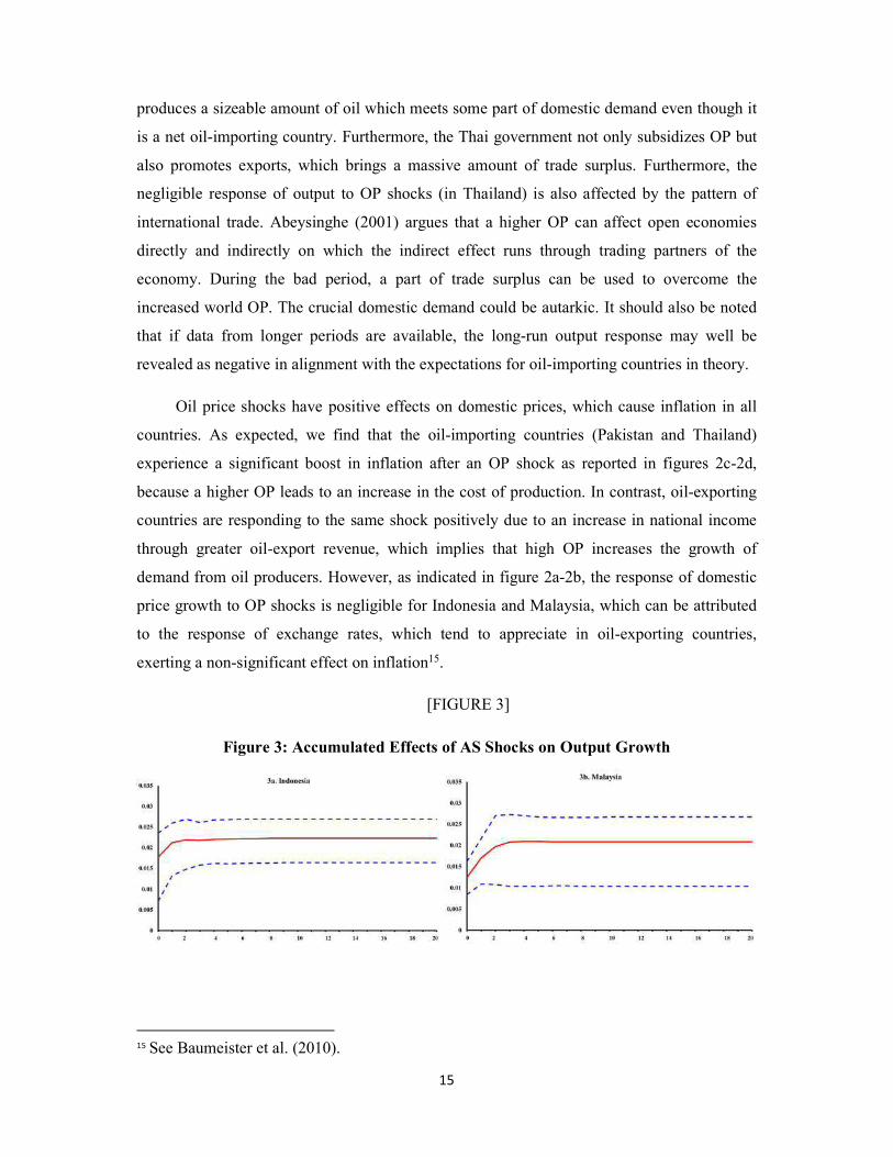
[FIGURE 3]

Figure 3: Accumulated Effects of AS Shocks on Output Growth

15 See Baumeister et al. (2010).

16

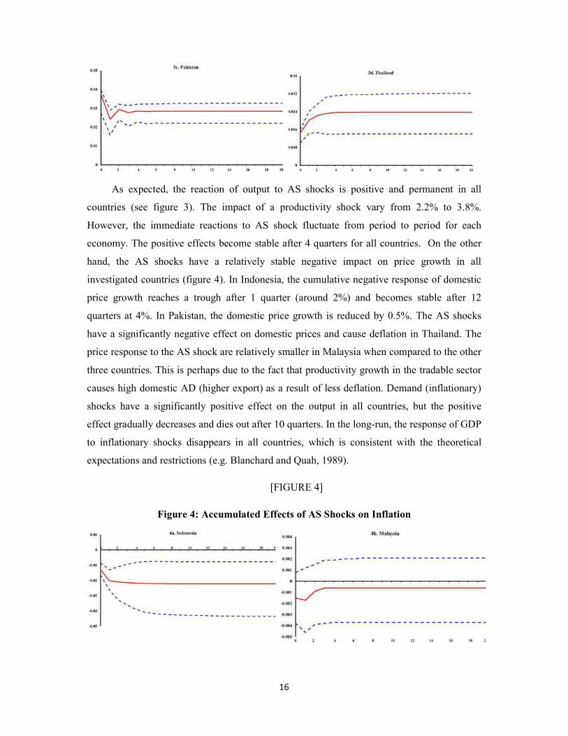
As expected, the reaction of output to AS shocks is positive and permanent in all

countries (see figure 3). The impact of a productivity shock vary from 2.2% to 3.8%.

However, the immediate reactions to AS shock fluctuate from period to period for each

economy. The positive effects become stable after 4 quarters for all countries. On the other

hand, the AS shocks have a relatively stable negative impact on price growth in all

investigated countries (figure 4). In Indonesia, the cumulative negative response of domestic

price growth reaches a trough after 1 quarter (around 2%) and becomes stable after 12

quarters at 4%. In Pakistan, the domestic price growth is reduced by 0.5%. The AS shocks

have a significantly negative effect on domestic prices and cause deflation in Thailand. The

price response to the AS shock are relatively smaller in Malaysia when compared to the other

three countries. This is perhaps due to the fact that productivity growth in the tradable sector

causes high domestic AD (higher export) as a result of less deflation. Demand (inflationary)

shocks have a significantly positive effect on the output in all countries, but the positive

effect gradually decreases and dies out after 10 quarters. In the long-run, the response of GDP

to inflationary shocks disappears in all countries, which is consistent with the theoretical

expectations and restrictions (e.g. Blanchard and Quah, 1989).

[FIGURE 4]

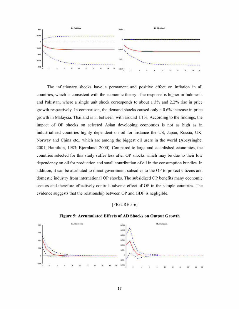
Figure 4: Accumulated Effects of AS Shocks on Inflation

17

The inflationary shocks have a permanent and positive effect on inflation in all

countries, which is consistent with the economic theory. The response is higher in Indonesia

and Pakistan, where a single unit shock corresponds to about a 3% and 2.2% rise in price

growth respectively. In comparison, the demand shocks caused only a 0.6% increase in price

growth in Malaysia. Thailand is in between, with around 1.1%. According to the findings, the

impact of OP shocks on selected Asian developing economics is not as high as in

industrialized countries highly dependent on oil for instance the US, Japan, Russia, UK,

Norway and China etc., which are among the biggest oil users in the world (Abeysinghe,

2001; Hamilton, 1983; Bjornland, 2000). Compared to large and established economies, the

countries selected for this study suffer less after OP shocks which may be due to their low

dependency on oil for production and small contribution of oil in the consumption bundles. In

addition, it can be attributed to direct government subsidies to the OP to protect citizens and

domestic industry from international OP shocks. The subsidized OP benefits many economic

sectors and therefore effectively controls adverse effect of OP in the sample countries. The

evidence suggests that the relationship between OP and GDP is negligible.

[FIGURE 5-6]

Figure 5: Accumulated Effects of AD Shocks on Output Growth

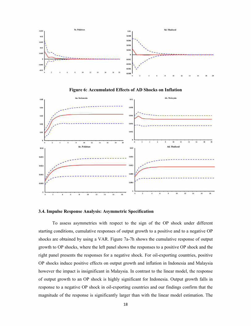
18

Figure 6: Accumulated Effects of AD Shocks on Inflation

3.4. Impulse Response Analysis: Asymmetric Specification

To assess asymmetries with respect to the sign of the OP shock under different

starting conditions, cumulative responses of output growth to a positive and to a negative OP

shocks are obtained by using a VAR. Figure 7a-7h shows the cumulative response of output

growth to OP shocks, where the left panel shows the responses to a positive OP shock and the

right panel presents the responses for a negative shock. For oil-exporting countries, positive

OP shocks induce positive effects on output growth and inflation in Indonesia and Malaysia

however the impact is insignificant in Malaysia. In contrast to the linear model, the response

of output growth to an OP shock is highly significant for Indonesia. Output growth falls in

response to a negative OP shock in oil-exporting countries and our findings confirm that the

magnitude of the response is significantly larger than with the linear model estimation. The

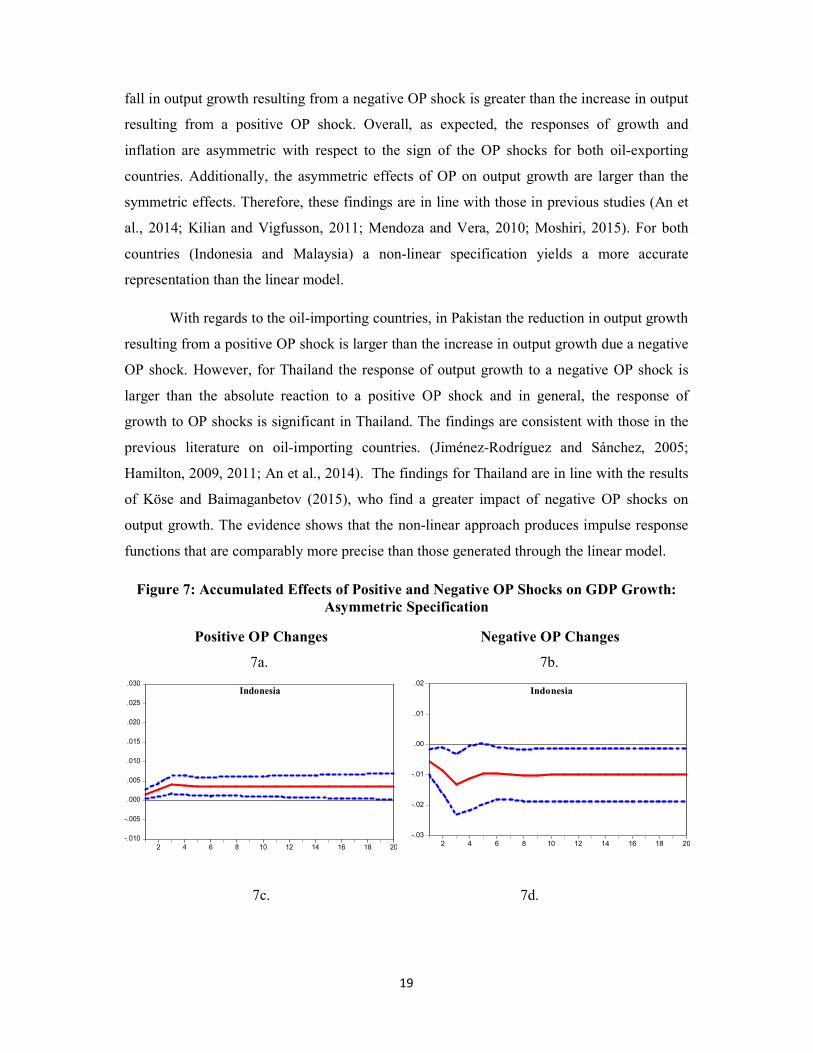
19

fall in output growth resulting from a negative OP shock is greater than the increase in output

resulting from a positive OP shock. Overall, as expected, the responses of growth and

inflation are asymmetric with respect to the sign of the OP shocks for both oil-exporting

countries. Additionally, the asymmetric effects of OP on output growth are larger than the

symmetric effects. Therefore, these findings are in line with those in previous studies (An et

al., 2014; Kilian and Vigfusson, 2011; Mendoza and Vera, 2010; Moshiri, 2015). For both

countries (Indonesia and Malaysia) a non-linear specification yields a more accurate

representation than the linear model.

With regards to the oil-importing countries, in Pakistan the reduction in output growth

resulting from a positive OP shock is larger than the increase in output growth due a negative

OP shock. However, for Thailand the response of output growth to a negative OP shock is

larger than the absolute reaction to a positive OP shock and in general, the response of

growth to OP shocks is significant in Thailand. The findings are consistent with those in the

previous literature on oil-importing countries. (Jiménez-Rodríguez and Sánchez, 2005;

Hamilton, 2009, 2011; An et al., 2014). The findings for Thailand are in line with the results

of Köse and Baimaganbetov (2015), who find a greater impact of negative OP shocks on

output growth. The evidence shows that the non-linear approach produces impulse response

functions that are comparably more precise than those generated through the linear model.

Figure 7: Accumulated Effects of Positive and Negative OP Shocks on GDP Growth: Asymmetric Specification

Positive OP Changes 7a.

Negative OP Changes 7b.

-.010

-.005

.000

.005

.010

.015

.020

.025

.030

2 4 6 8 10 12 14 16 18 20

Indonesia

-.03

-.02

-.01

.00

.01

.02

2 4 6 8 10 12 14 16 18 20

Indonesia

7c. 7d.

20

-.015

-.010

-.005

.000

.005

.010

.015

.020

2 4 6 8 10 12 14 16 18 20

Malaysia

-.020

-.015

-.010

-.005

.000

.005

.010

.015

.020

2 4 6 8 10 12 14 16 18 20

Malaysia

7e. 7f.

-.04

-.02

.00

.02

.04

.06

2 4 6 8 10 12 14 16 18 20

Pakistan

-.04

-.03

-.02

-.01

.00

.01

.02

.03

.04

2 4 6 8 10 12 14 16 18 20

Pakistan

7g. 7h.

-.08

-.06

-.04

-.02

.00

.02

.04

.06

.08

2 4 6 8 10 12 14 16 18 20

Thailand

-.02

-.01

.00

.01

.02

.03

.04

2 4 6 8 10 12 14 16 18 20

Thailand

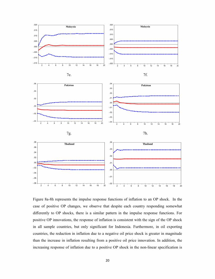
Figure 8a-8h represents the impulse response functions of inflation to an OP shock. In the

case of positive OP changes, we observe that despite each country responding somewhat

dierently to OP shocks, there is a similar pattern in the impulse response functions. For

positive OP innovations, the response of inflation is consistent with the sign of the OP shock

in all sample countries, but only significant for Indonesia. Furthermore, in oil exporting

countries, the reduction in inflation due to a negative oil price shock is greater in magnitude

than the increase in inflation resulting from a positive oil price innovation. In addition, the

increasing response of inflation due to a positive OP shock in the non-linear specification is

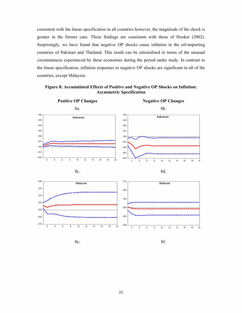
21

consistent with the linear specification in all countries however, the magnitude of the shock is

greater in the former case. These findings are consistent with those of Hooker (2002).

Surprisingly, we have found that negative OP shocks cause inflation in the oil-importing

countries of Pakistan and Thailand. This result can be rationalised in terms of the unusual

circumstances experienced by these economies during the period under study. In contrast to

the linear specification, inflation responses to negative OP shocks are significant in all of the

countries, except Malaysia.

Figure 8: Accumulated Effects of Positive and Negative OP Shocks on Inflation: Asymmetric Specification

Positive OP Changes 8a.

Negative OP Changes 8b.

-.002

-.001

.000

.001

.002

.003

.004

.005

.006

2 4 6 8 10 12 14 16 18 20

Indonesia

-.004

-.003

-.002

-.001

.000

.001

.002

.003

.004

2 4 6 8 10 12 14 16 18 20

Indonesia

8c. 8d.

-.010

-.005

.000

.005

.010

.015

.020

2 4 6 8 10 12 14 16 18 20

Malaysia

-.008

-.004

.000

.004

.008

.012

2 4 6 8 10 12 14 16 18 20

Malaysia

8e. 8f.

22

-.08

-.04

.00

.04

.08

.12

2 4 6 8 10 12 14 16 18 20

Pakistan

-.02

-.01

.00

.01

.02

.03

.04

.05

.06

2 4 6 8 10 12 14 16 18 20

Pakistan

g. h.

-.02

-.01

.00

.01

.02

.03

.04

2 4 6 8 10 12 14 16 18 20

Thailand

-.005

.000

.005

.010

.015

.020

2 4 6 8 10 12 14 16 18 20

Thailand

3.4 Forecast Error Variance Decomposition: Linear Specification

In this subsection, we study the forecast error variance decompositions (FEVDs), which

allow us to verify how much of the forecast error variance is explained by shocks to each

explanatory variable in a system over a time period. Variance decomposition is based on

structural decomposition (orthogonalization) estimated in the factorization matrices for the

identified VAR model. For each country in this study, variance decomposition is used to

measure the proportion of fluctuations in output caused by OP, AS and AD shocks. Tables 2-

5 show the variance decompositions of the linear specification.

[TABLE 2]

Table 2: Forecast-Error Variance Decompositions of Output Growth and Inflation Indonesia: Linear Specification

Horizon Output Growth Inflation (quarters) OP shock AS shock AD shock OP shock AS shock AD shock

1 0.0 41.0 59.0 0.0 69.0 31.0 2 3.0 34.0 63.0 0.0 65.0 34.0 3 3.0 33.0 64.0 0.0 50.0 49.0 4 3.0 33.0 64.0 0.0 49.0 51.0

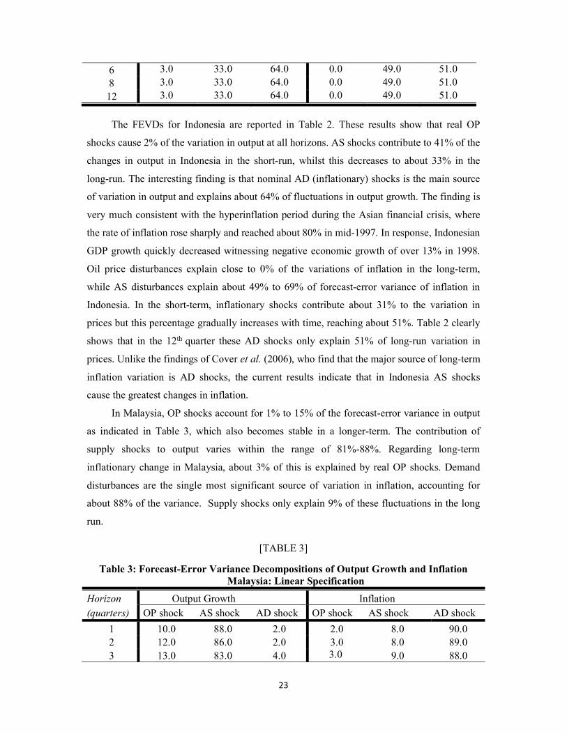
23

6 3.0 33.0 64.0 0.0 49.0 51.0 8 3.0 33.0 64.0 0.0 49.0 51.0

12 3.0 33.0 64.0 0.0 49.0 51.0

The FEVDs for Indonesia are reported in Table 2. These results show that real OP

shocks cause 2% of the variation in output at all horizons. AS shocks contribute to 41% of the

changes in output in Indonesia in the short-run, whilst this decreases to about 33% in the

long-run. The interesting finding is that nominal AD (inflationary) shocks is the main source

of variation in output and explains about 64% of fluctuations in output growth. The finding is

very much consistent with the hyperinflation period during the Asian financial crisis, where

the rate of inflation rose sharply and reached about 80% in mid-1997. In response, Indonesian

GDP growth quickly decreased witnessing negative economic growth of over 13% in 1998.

Oil price disturbances explain close to 0% of the variations of inflation in the long-term,

while AS disturbances explain about 49% to 69% of forecast-error variance of inflation in

Indonesia. In the short-term, inflationary shocks contribute about 31% to the variation in

prices but this percentage gradually increases with time, reaching about 51%. Table 2 clearly

shows that in the 12th quarter these AD shocks only explain 51% of long-run variation in

prices. Unlike the findings of Cover et al. (2006), who find that the major source of long-term

inflation variation is AD shocks, the current results indicate that in Indonesia AS shocks

cause the greatest changes in inflation.

In Malaysia, OP shocks account for 1% to 15% of the forecast-error variance in output

as indicated in Table 3, which also becomes stable in a longer-term. The contribution of

supply shocks to output varies within the range of 81%-88%. Regarding long-term

inflationary change in Malaysia, about 3% of this is explained by real OP shocks. Demand

disturbances are the single most significant source of variation in inflation, accounting for

about 88% of the variance. Supply shocks only explain 9% of these fluctuations in the long

run.

[TABLE 3]

Table 3: Forecast-Error Variance Decompositions of Output Growth and Inflation Malaysia: Linear Specification

Horizon Output Growth Inflation (quarters) OP shock AS shock AD shock OP shock AS shock AD shock

1 10.0 88.0 2.0 2.0 8.0 90.0 2 12.0 86.0 2.0 3.0 8.0 89.0 3 13.0 83.0 4.0 3.0 9.0 88.0

24

4 15.0 81.0 4.0 3.0 9.0 88.0 6 15.0 81.0 4.0 3.0 9.0 88.0 8 15.0 81.0 4.0 3.0 9.0 88.0

12 15.0 81.0 4.0 3.0 9.0 88.0

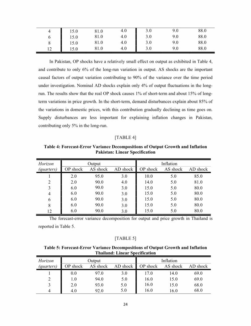
In Pakistan, OP shocks have a relatively small effect on output as exhibited in Table 4,

and contribute to only 6% of the long-run variation in output. AS shocks are the important

causal factors of output variation contributing to 90% of the variance over the time period

under investigation. Nominal AD shocks explain only 4% of output fluctuations in the long-

run. The results show that the real OP shock causes 1% of short-term and about 15% of long-

term variations in price growth. In the short-term, demand disturbances explain about 85% of

the variations in domestic prices, with this contribution gradually declining as time goes on.

Supply disturbances are less important for explaining inflation changes in Pakistan,

contributing only 5% in the long-run.

[TABLE 4]

Table 4: Forecast-Error Variance Decompositions of Output Growth and Inflation Pakistan: Linear Specification

Horizon Output Inflation (quarters) OP shock AS shock AD shock OP shock AS shock AD shock

1 2.0 95.0 3.0 10.0 5.0 85.0 2 2.0 90.0 4.0 14.0 5.0 81.0 3 6.0 90.0 3.0 15.0 5.0 80.0 4 6.0 90.0 3.0 15.0 5.0 80.0 6 6.0 90.0 3.0 15.0 5.0 80.0 8 6.0 90.0 3.0 15.0 5.0 80.0

12 6.0 90.0 3.0 15.0 5.0 80.0 The forecast-error variance decomposition for output and price growth in Thailand is

reported in Table 5.

[TABLE 5]

Table 5: Forecast-Error Variance Decompositions of Output Growth and Inflation Thailand: Linear Specification

Horizon Output Inflation (quarters) OP shock AS shock AD shock OP shock AS shock AD shock

1 0.0 97.0 3.0 17.0 14.0 69.0 2 1.0 94.0 5.0 16.0 15.0 69.0 3 2.0 93.0 5.0 16.0 15.0 68.0 4 4.0 92.0 5.0 16.0 16.0 68.0

25

6 4.0 92.0 5.0 16.0 16.0 68.0 8 4.0 92.0 5.0 16.0 16.0 68.0

12 4.0 92.0 5.0 16.0 16.0 68.0

In terms of variance decomposition of output, AS shocks contribute the biggest

proportion in Thailand. The short run effect is 97% which gradually decreases with the

forecast horizon to 92%. In the long-run, OP and AD shocks account for 4% and 5% of the

variation of output respectively. Supply shocks in Thailand account for a sizable fluctuation

in inflation representing about 16% of the long-term variability. Real OP disturbances explain

about 16% of the variation in inflation and demand disturbances describe about 68%.

To summarise the FEVD results, the study concludes that AS disturbances are the most

important factor behind output movements in both short-term and long-term in this set of

countries except in Indonesia. It seems that the inflationary (AD) shocks are the main source

variation in output for Indonesia. It suggests that the recession in the Indonesia during 1997-

98 was dominated by inflationary disturbances. For all four countries, output behaviour

seems consistent with real business cycle theory. Demand is the main determinant of the

variability in domestic prices in Malaysia, Pakistan and Thailand. In Indonesia, supply shocks

are more dominant than demand shocks in explaining domestic price fluctuations. In all

countries, the demand, and supply shocks are a significant source of business cycles.

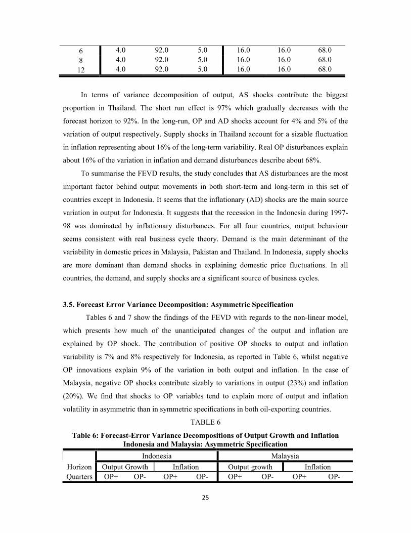
3.5. Forecast Error Variance Decomposition: Asymmetric Specification Tables 6 and 7 show the findings of the FEVD with regards to the non-linear model,

which presents how much of the unanticipated changes of the output and inflation are

explained by OP shock. The contribution of positive OP shocks to output and inflation

variability is 7% and 8% respectively for Indonesia, as reported in Table 6, whilst negative

OP innovations explain 9% of the variation in both output and inflation. In the case of

Malaysia, negative OP shocks contribute sizably to variations in output (23%) and inflation

(20%). We nd that shocks to OP variables tend to explain more of output and inflation

volatility in asymmetric than in symmetric specications in both oil-exporting countries.

TABLE 6

Table 6: Forecast-Error Variance Decompositions of Output Growth and Inflation Indonesia and Malaysia: Asymmetric Specification

Indonesia Malaysia Horizon Output Growth Inflation Output growth Inflation Quarters OP+ OP- OP+ OP- OP+ OP- OP+ OP-

26

1 4.0 3.0 5.0 3.0 1.0 26.0 0.0 4.0 2 5.0 4.0 5.0 4.0 2.0 22.0 5.0 9.0 3 7.0 9.0 8.0 9.0 7.0 22.0 5.0 19.0 4 7.0 9.0 8.0 9.0 8.0 22.0 5.0 20.0 6 7.0 9.0 8.0 9.0 8.0 23.0 5.0 20.0 8 7.0 9.0 8.0 9.0 8.0 23.0 5.0 20.012 7.0 9.0 8.0 9.0 8.0 23.0 5.0 20.0

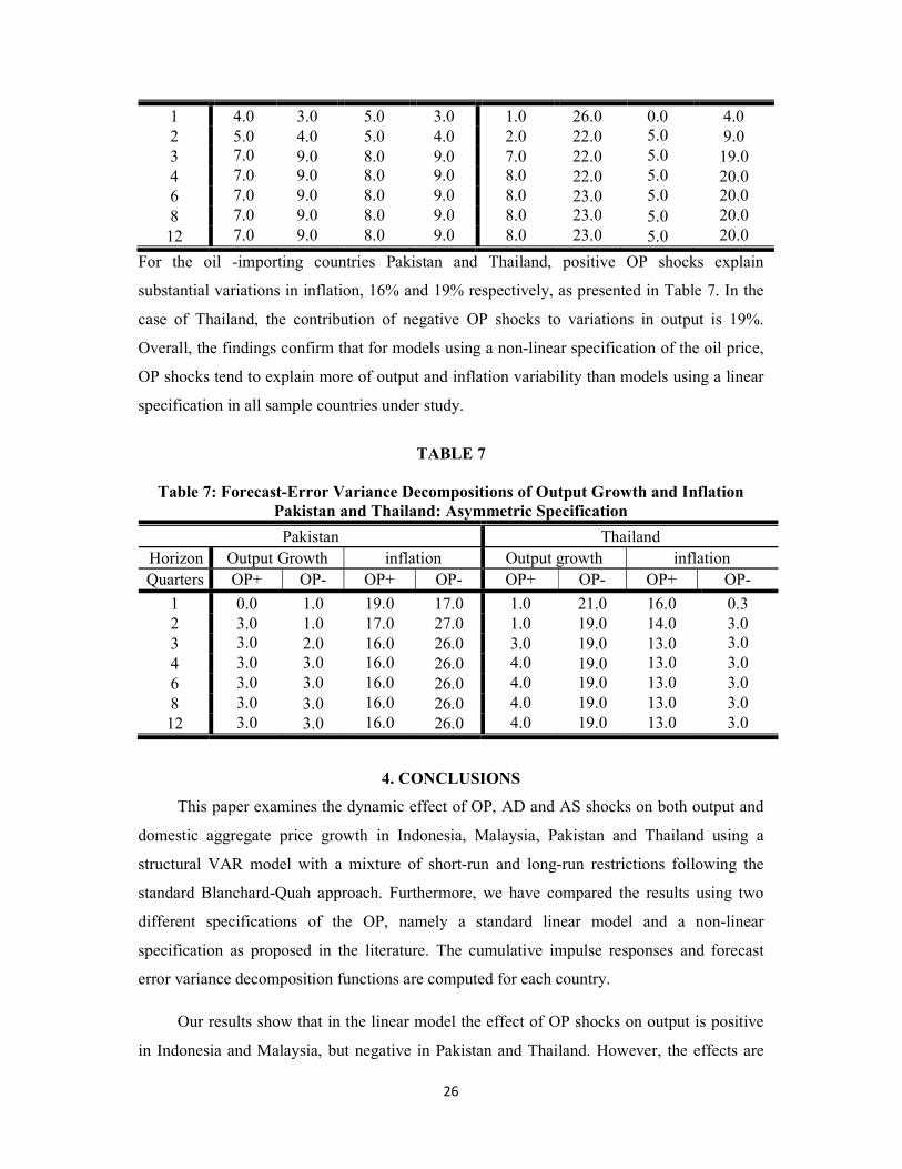
For the oil -importing countries Pakistan and Thailand, positive OP shocks explain

substantial variations in inflation, 16% and 19% respectively, as presented in Table 7. In the

case of Thailand, the contribution of negative OP shocks to variations in output is 19%.

Overall, the findings confirm that for models using a non-linear specification of the oil price,

OP shocks tend to explain more of output and inflation variability than models using a linear

specification in all sample countries under study.

TABLE 7

Table 7: Forecast-Error Variance Decompositions of Output Growth and Inflation Pakistan and Thailand: Asymmetric Specification

Pakistan Thailand Horizon Output Growth inflation Output growth inflation Quarters OP+ OP- OP+ OP- OP+ OP- OP+ OP-

1 0.0 1.0 19.0 17.0 1.0 21.0 16.0 0.3 2 3.0 1.0 17.0 27.0 1.0 19.0 14.0 3.0 3 3.0 2.0 16.0 26.0 3.0 19.0 13.0 3.04 3.0 3.0 16.0 26.0 4.0 19.0 13.0 3.06 3.0 3.0 16.0 26.0 4.0 19.0 13.0 3.0 8 3.0 3.0 16.0 26.0 4.0 19.0 13.0 3.0 12 3.0 3.0 16.0 26.0 4.0 19.0 13.0 3.0

4. CONCLUSIONS This paper examines the dynamic effect of OP, AD and AS shocks on both output and

domestic aggregate price growth in Indonesia, Malaysia, Pakistan and Thailand using a

structural VAR model with a mixture of short-run and long-run restrictions following the

standard Blanchard-Quah approach. Furthermore, we have compared the results using two

different specifications of the OP, namely a standard linear model and a non-linear

specification as proposed in the literature. The cumulative impulse responses and forecast

error variance decomposition functions are computed for each country.

Our results show that in the linear model the effect of OP shocks on output is positive

in Indonesia and Malaysia, but negative in Pakistan and Thailand. However, the effects are

27

insignificant for all countries. These results are consistent with the findings of Ran and Voon

(2012), who concluded that OPs do not have a significant effect on economic activity in East

Asian countries. When using the nonlinear model, in contrast to the linear model, we find that

positive and negative OP shocks separately have significant effects on output and inflation in

Indonesia. Additionally, we observe that OP shocks have a significant impact on inflation in

Pakistan and Thailand. Overall, the findings confirm that OP changes have larger effects on

macroeconomic variables when a non-linear model is used as opposed to the standard linear

model in all four economies. The evidence also shows that positive OP innovations have

dierent impacts on output growth and inflation to those of negative innovations. This

contrasts with the linear model in which OPs are assumed to have symmetrical impacts on

real activity.

The findings of the current study also suggest that OP increases causes inflation in all

countries, which corresponds to an earlier conjecture in section 2. This is consistent with the

finding of Abeysinghe (2001) and Cunado and Perez de Gracia (2005) that even oil-exporting

countries such as Indonesia and Malaysia couldn’t evade the adverse repercussions of high

OPs. The inflationary consequences for oil-exporters are negligible, possibly because of the

exchange rate appreciation in the aftermath of an OP shock. The results of OP shocks are

particularly negative for oil-importers, as they may bear losses because of the high input cost.

On the other hand, oil-exporters may experience some benefits and revenue increases but also

suffer high inflation. Although our variance decomposition investigation suggests that OPs

have a role in explaining output and inflation volatility in all sample economies, our findings

suggest that OP shocks are more likely to cause fluctuations in the macroeconomic variables

of some countries than in others. The relatively small or negligible effect found for some

countries could be attributed to government direct control and subsidised OPs which help to

minimize the adverse effect of OP on real activities and to avoid a sharp decline in GDP and

high inflation in response to positive OP shocks. In addition, the economic structure of a

country plays a crucial role, which may affect the influence of OP shocks on macroeconomic

fluctuations. Countries with a low production reliance on oil, a low share of oil in the

consumption bundle and relatively low labour intensities in production are expected to suffer

less from OP shocks. Shocks of AD demand and AS have played a significant role in

explaining recessions, particularly the 1997-98 recession in East Asian countries. For the

recession experienced in 2008-09 the OP had little impact and the recession was largely

caused by other disturbances in all countries.

28

In alignment with conventional wisdom, productivity (AS) shocks are the key reason

for fluctuations in output and nominal AD shocks are the main factor inducing fluctuations in

aggregate price growth in all countries except in Indonesia. In Indonesia, demand

disturbances are more important than supply disturbances in explaining output fluctuations

and interestingly, productivity shocks are the main reason for fluctuations in aggregate price

growth in Indonesia because its economy is highly dependent on exports. These findings may

suggest that output growth of the trade sector is higher than that in non-trade sectors in

Indonesia. The findings confirmed all the restrictions imposed by the model to identify the

different shocks. Most of the dynamic changes of the macroeconomic variables are in line

with the economic model, and the shocks fit well with actual events that have occurred in the

various countries.

These findings carry significant policy recommendations to governments, suggesting

the need for comprehensive reforms of OP and oil subsidy policies. The government policies

should pay more attention to emerging new and advanced solutions to achieve OP stability.

Many countries increase oil subsidies in order to minimize the damaging effects of OP

increases on poor people however the consequences of OP stabilization policies are budget

deficit16 and pollution. The policy should be implemented in such a way so as to reduce OP

shocks to the economy and minimize budget deficit. This suggests that the removal of oil

subsidies should be gradual because people could recognize policies and become more

resilient to OP shocks. Furthermore, in order to control inflation, the monetary policy

response to an OP shock could involve raising the interest rate to reduce consumer and

investment spending.

Furthermore, such results have other significant implications, in particular that the

identification and decomposition of demand and supply shocks are crucial. This enables

better analysis of the effects of monetary and fiscal policy on the economy, which is in turn

taken as a measure of progress of the growth and improvement of market mechanisms. It

could also help these countries walk out of budget deficit and achieve a balanced budget,

which will substantially reduce the risk of falling into financial crisis again.

Overall, for a fuller understanding of recent developments in the economies that have

been considered, and in order to structure economic policies that aim at stabilizing the

macroeconomy, the results of the current study should be carefully taken into account during

16 Rafiq et al. (2009) examined the impact of OP shocks on economic activity in Thailand by employing a VARmodel. Using quarterly data from 1993q1 to 2006q4 they found a structural break in the time series data during the Asian financial crisis of 1997-1998. They also found that the budget deficit originated mainly from movements in OPs during the post crisis period, which may have been due to the floating exchange rate policy.

29

the design and improvement of economic policies. This is particularly relevant for Asian

countries, where (productivity) supply and inflationary shocks are the main source of

variation in economic activities.

30

REFERENCES

Abeysinghe, T. 2001. Estimation of Direct and Indirect Impact of Oil Price on Growth. Economics Letters, 73, 147-153.

An, L., Jin, X., Ren, X. 2014. Are the Macroeconomic Effects of Oil Price Shock Symmetric? A Factor-augmented Vector Autoregressive Approach. Energy Economics, 45, 217-228.

Barsky, R.B. and L. Kilian, 2004. Oil and the Macroeconomy since the 1970s. Journal of Economic Perspectives, 18, 115-134. Baumeister, C., G. Peersman and I. Van Robays, 2010. The economic consequences of oil shocks: Differences across countries and time. Inflation in an era of relative price shocks. Fry, Jones and Kent (eds), Reserve Bank of Australia, 91-128.

Bjornland, H.C. 2000. The Dynamic Effects of Aggregate Demand, Supply and Oil Price Shocks-A Comparative Study. The Manchester School, 68, 578-607.

Bjornland, H.C., 2009. Oil Price Shocks and Stock Market Booms in an Oil Exporting Country. Scottish Journal of Political Economy, 56, 232-254.

Blanchard, O.J and D. Quah, 1989. The Dynamic Effects of Aggregate Demand and Supply Disturbances. American Economic Review, 79, 655-673.

Blanchard, O.J and J. Gali, 2010. The Macroeconomic Effects of Oil Price Shocks: Why are the 2000s So Different from the 1970s?, in International Dimensions of Monetary Policy 373-421. Gali, J. and Gertler, M. eds., University of Chicago Press, Chicago.

Brown, S.P.A., M.K. Yucel, and J. Thompson, 2004. Business Cycles: the Role of Energy Prices, in: Cutler, J. Cleveland (Ed.), Encyclopaedia of Energy, Academy Press.

Cover, J.P., W. Enders, and C.J. Hueng, 2006. Using the Aggregate Demand-Aggregate Supply Model to Identify Structural Demand-Side and Supply-Side Shocks: Results Using a Bivariate VAR. Journal of Money Credit and Banking, 38, 777-790.

Cunado, J. and F. Perez de Gracia, 2003. Do Oil Price Shocks Matter? Evidence from Some European Countries. Energy Economics, 25, 137-154.

Cunado, J. and F. Perez de Gracia, 2005. Oil price, Economic Activity and Inflation: Evidence for Some Asian Countries. Quarterly Review of Economics and Finance, 45, 65-83.

Elder, J. and A. Serletis, 2010. Oil Price Uncertainty. Journal of Money, Credit and Banking, 42, 1137-1159.

Hamilton, J.D., 1983. Oil and the Macroeconomy since World War II. Journal of Political Economy, 91, 228-248.

Hamilton, J.D., 1996. This is what Happened to the Oil Price-Macroeconomy Relationship. Journal of Monetary Economics, 38, 215-220.

31

Hamilton, J.D., 2003. What is an Oil Shock? Journal of Econometrics, 113, 363-398.

Hamilton, J.D., 2009. Causes and consequences of the oil shock of 2007-08, Brookings Papers on Economic Activity, 40, 215–283.

Hamilton, J.D., 2011. Nonlinearities and the Macroeconomic Effects of Oil Prices, Macroeconomic Dynamics, 15, 364-378.

Hooker, M. (2002). Are Oil Shocks Inflationary? Asymmetric and Nonlinear Specifications Versus Change in Regime. Journal of Money, Credit and Banking, 34, 540-561.

Hsing, Y., 2012. Impacts of Macroeconomic Forces and External Shocks on Real Output for Indonesia. Economic Analysis & Policy, 42, 97-104.

Ito, K., 2008. Oil Price and the Russian Economy: A VEC Model Approach. International Research Journal of Finance and Economics, 17, 68-74.

Jimenez-Rodriguez, R. and M. Sanchez, 2005. Oil Price Shocks and Real GDP Growth: Empirical Evidence for Some OECD countries, Applied Economics, 37, 201-228.

Kilian, L., 2008. Exogenous Oil Supply Shocks: How Big Are They and How Much Do They Matter for the U.S. Economy? Review of Economics and Statistics, 90, 216-240.

Kilian, L., 2009. Not All Oil Price Shocks Are Alike: Disentangling Demand and Supply Shocks in the Crude Oil Market. American Economic Review, 99, 1053-1069.

Kilian, L. and Vigfusson, R.J., 2011. Are the Responses of the U.S. Economy Symmetric in Energy Rrice increases and decreases? Quantitative Economics, 2, 419–453.

Kilian, L. and J.V. Vigfusson, 2013. Do Oil Prices Help Forecast US Real GDP? The Role of Nonlinearities and Asymmetries. Journal of Business & Economic Statistics, 31, 78-93.

Köse, N., Baimaganbetov, S. (2015). The asymmetric impact of oil price shocks on Kazakhstan macroeconomic dynamics: A structural vector autoregression approach. International Journal of Energy Economics and Policy, 5, 1058-1064.

Lescaroux, F. and V. Mignon, 2009. The Symposium on 'China's Impact on the Global Economy': Measuring the Effects of Oil Prices on China's Economy: A Factor-Augmented Vector Autoregressive Approach. Pacific Economic Review, 14, 410-425.

Lee, K., N. Shawn, and R. Ratti 1995. Oil Shocks and the Macroeconomy: The Role of Price Variability. Energy Journal, 16, 39–56.

Lee, K., Ni, S. 2002. On the dynamic effects of oil price shocks: A study using industry level data. Journal of Monetary Economics, 49, 823-852.

Mendoza, O. and D. Vera (2010). The Asymmetric Effects of Oil Shocks on an Oil Exporting Economy. Cuadernos De Economia, 47, 3-13.

Moshiri, S. (2015). Asymmetric Effects of Oil Price Shocks in Oil-Exporting Countries: The Role of Institutions, OPEC Energy Review, 39, 222-246.

32

Mork, K., 1989. Oil and the Macroeconomy when Prices Go Up and Down: An Extension of Hamilton’s Results. Journal of Political Economy, 97, 740-744. Prambudia, Y. and M. Nakano, 2012. Exploring Malaysia’s Transformation to Net Oil Importer and Oil Import Dependence. Energies, 8, 2989-3018.

Ng, S. and P. Perron 2001. Lag Length selection and the Construction of Unit Root Tests with Good Size and Power. Econometrica, 69, 1519-1554.

Rafiq, S., R. Salim and H. Bloch, 2009. Impact of Crude Oil Price Volatility on Economic Activities: An Empirical Investigation in the Thai Economy. Journal of Resources Policy, 34, 121-132.

Ran, J. and J.P. Voon, 2012. Does oil price shock affect small open economies? Evidence from Hong Kong, Singapore, South Korea and Taiwan. Applied Economics Letters, 19, 1599-1602.

Rautava, J., 2004. The Role of Oil Prices and the Real Exchange Rate in Russia’s Economy – A cointegration approach. Journal of Comparative Economics, 32, 315-327.

Rotemberg, J.J. and M. Woodford, 1996. Imperfect Competition and the Effects of Energy Price Increases on Economic Activity. Journal of Money, Credit, and Banking, 28, 550–77.

Schmitz, T., J.L. Seale and P. J. Buzzanell, 2007. Brazil’s Domination of the World’s Sugar Market. Arizona State University, Working Paper.

Schneider, M., 2004. The Impact of Oil Price Changes on Growth and Inflation. Austrian Central Bank, 2, 27-36.

Schubert, S.F. and S.J. Turnovsky, 2011. The Impact of Oil Prices on An Oil-importing Developing Economy. Journal of Development Economics, 94, 18-29.

Salim, R. and S. Rafiq, 2011. The impact of crude oil price volatility on selected Asian emerging economies. Global Business and Social Science Research Conference, Beijing, China, 1-33.

Tang, W., L. Wu and Z. Zhang, 2010. Oil Price Shocks and their Short- and Long-term effects on the Chinese Economy. Energy Economics, 32, S3-14.

Zivot, E. and D. Andrews. 1992. Further Evidence of Great Crash, the oil price shock and unit root hypothesis. Journal of Business and Economic Statistics, 10, 251-270.

33

APPENDIX A

Table A1: Unit Root Test

Variables

Augmented Dickey-Fuller (ADF) Test Phillips-Perron (PP) Test

Indonesia Malaysia Pakistan Thailand Indonesia Malaysia Pakistan Thailand

Real oil price ( tOP) -2.969+ -2.127 -1.944 -1.533 -2.381 -2.347 -1.749 -1.594

Oil price growth ( tOPΔ ) -8.745+++ -8.420+++ -8.839+++ -7.569+++ -8.985+++ -8.786+++ -8.843+++ -7.736+++

Real GDP ( )GDP

Growth ( )

-1.973

-8.282 +++

-3.182

-4.901 +++

-1.381

-14.487+++

-2.480

-10.490+++

-1.905

-8.272+++

-2.897

-11.584+++

-1.701

-14.723+++

-2.5787

10.454+++

Consumer prices ( )

Inflation ( )

-2.068

-8.295+++

-2.780

-8.705+++

-1.839

-3.256++

-2.259

-6.565+++

-1.989

-8.295+++

-2.774

-8.642+++

-1.579

-5.429+++

-1.971

-6.101+++

Note: +++, ++ and + indicate the growth of significance at the 1%, 5% and 10% respectively. Constant and time trend are used for the variables at growth, while only constant is

included for variables at the first order difference.

ty

ty

tp

tp

34

Table A2: Summary of the Unit Root Tests for Output and Inflation with and without Structural Breaks

Indonesia Malaysia

Tests tOPΔ tOPΔZA -8.564*** -8.690*** -8.695*** -9.043*** -5.925*** -8.449***

MZa -37.745*** -49.089*** -49.164*** -46.919*** -49.400*** -39.008 MSB -4.342*** -4.954*** -4.958*** -4.817*** -4.966*** -4.407MZT 0.115*** 0.101*** 0.101*** 0.103*** 0.101*** 0.113RMT 0.656*** 0.500*** 0.499*** 0.593*** 0.506*** 0.655

Pakistan Thailand

Tests tOPΔ tOPΔZA -9.821*** -15.328*** -4.415*** -8.212*** -12.676*** -5.633***

MZa -9.261*** -45.043*** -12.604*** -43.258*** -44.454*** -34.965***

MSB -2.152*** -4.745*** -2.426*** -4.640*** -4.714*** -4.135***

MZT 0.232*** 0.105*** 0.193*** 0.107*** 0.106*** 0.118***

RMT 2.646*** 0.547*** 2.275*** 0.596*** 0.551*** 0.838***

Note: ***, ** and * indicate the growth of significance at the 1%, 5% and 10% respectively. For M unit root tests the MAIC information criterion is used to select the autoregressive truncation lag, k, as proposed in Ng and Perron (2001). is the Zivot-Andrews unit root test. MPT is the Elliot-Rothemberg-Stock unit root test. ADF-GLS is the Elliot, Rothemberg and Stock unit root test. The critical values are taken from Ng and Perron (2001).

Table A3: Cointegration Test Results with Trace and Maximum Eigenvalues Statistics

(a) Indonesia

Trace Test Maximum Eigenvalues Hypothesised Statistics Critical

Values 5% Statistics Critical

Values 5% No. of CE(s) None 29.120 29.797 20.675 21.132 At most 1 8.445 15.495 7.333 14.265 At most 2 1.112 3.841 1.112 3.841

(b) Malaysia

Trace Test Maximum Eigenvalues Hypothesised Statistics Critical

Values 5% Statistics Critical

Values 5% No. of CE(s) None 22.064 29.797 15.409 21.132 At most 1 6.654 15.495 5.007 14.265 At most 2 1.647 3.841 1.647 3.841

ty tp ty tp

ty tp ty tp

35

(c) Pakistan

Trace Test Maximum Eigenvalues Hypothesised Statistics Critical

Values 5% Statistics Critical

Values 5% No. of CE(s)None 20.332 29.797 15.313 21.132 At most 1 5.019 15.495 4.288 14.265 At most 2 0.731 3.841 0.731 3.841

(d) Thailand

Trace Test Maximum Eigenvalues Hypothesised Statistics Critical

Values 5% Statistics Critical

Values 5% No. of CE(s)None 32.698 29.797 24.707 21.132 At most 1 7.992 15.495 14.265 14.265 At most 2 1.889 3.841 1.889 3.841

Table A4: VAR Granger Causality/Block Exogeneity Wald Tests (p-values)

Country GDP growth does not Granger cause Oil price growth

Inflation does not Granger cause Oil price growth

Indonesia 0.92 0.94

Malaysia 0.46 0.01

Pakistan 0.22 0.51

Thailand 0.23 0.01