Submitted to Operations Researchmanuscript (Please, provide the mansucript number!)
Basis Paths and a Polynomial Algorithm for theMulti-Stage Production-Capacitated Lot-Sizing
Problem
Hark-Chin HwangDepartment of Industrial Engineering, Chosun University
375 Seosuk-Dong, Dong-Gu, Gwangju 501-759, South Korea, [email protected]
Hyun-soo AhnDepartment of Operations and Management Science, Ross School of Business, University of Michigan, Ann Arbor MI 48109,
Philip KaminskyDepartment of Industrial Engineering and Operations Research, University of California, Berkeley CA 94720,
We consider the multi-level lot-sizing problem with production capacities (MLSP-PC), in which production
and transportation decisions are made for a serial supply chain with capacitated production and concave
cost functions. Existing approaches to the multi-stage version of this problem are limited to non-speculative
cost functions – up to now, no polynomial algorithm for the multi-stage version of this model with general
concave cost functions has been developed. In this paper, we develop the first polynomial algorithm for the
MLSP-PC with general concave costs at all of the stages, and introduce a novel approach to overcome the
limitations of previous approaches. In contrast to traditional approaches to lot-sizing problems, in which the
problem is decomposed by time periods and is analyzed unidirectionally in time, we solve the problem by
introducing the concept of a basis path, which is characterized by time and stage. Our dynamic programming
algorithm proceeds both forward and backward in time along this basis path, enabling us to solve the problem
in polynomial time.
Key words : lot-sizing; production capacity; inventory and logistics; algorithms
1. Introduction
In the deterministic multi-level lot-sizing problem with production capacities (MLSP-PC), the
optimal manufacturing and distribution plan is determined for a centralized serial supply chain
with a capacitated manufacturing stage, several intermediate distribution stages (representing a
distribution center, wholesaler, etc), and a final retail stage. This optimal plan specifies produc-
tion quantities for the manufacturing stage of the supply chain, and a distribution plan for the
entire supply chain to meet time-varying demand that minimizes total cost, including production,
transportation, and inventory holding costs.
1

Author: Polynomial Algorithm for the Capacitated Multi-Stage Lot-Sizing2 Article submitted to Operations Research; manuscript no. (Please, provide the mansucript number!)
The single-stage uncapacitated lot-sizing problem was introduced by Wagner and Whitin (1958),
and efficient solution algorithms were designed by Federgruen and Tzur (1991), Wagelmans et
al. (1992) and Aggarwal and Park (1993). The multi-stage version of the uncapacitated problem
was solved by Zangwill (1968). Florian and Klein (1971) addressed the capacitated single-stage
version of the problem (see also Chung and Lin 1988; van Hoesel and Wagelmans 1996). Optimal
algorithms for the multi-stage problem with production capacity were first presented by Kaminsky
and Simchi-Levi (2003) for the two-stage case (2LSP-PC). Van Hoesel et al. (2005) generalized
the 2LSP-PC to the multi-stage lot-sizing problem MLSP-PC and Sargut and Romeijn (2007)
extended the 2LSP-PC to allow for subcontracting. For a two-stage lot-sizing model with outbound
transportation, Lee et al. (2003) consider cargo capacity constraints.
In this paper, we consider the MLSP-PC with general concave costs. For the version of the
problem with an affine transportation cost function, linear inventory costs, and no speculative
motive (which we will refer to as a non-speculative transportation cost structure or simply a non-
speculative cost structure for the remainder of the paper), van Hoesel et al. (2005) developed
a polynomial time algorithm, specifically an O(LT 4 + T 7) algorithm where L is the number of
stages in the supply chain and T is the length of the planning horizon. For models with general
concave production, transportation, and inventory costs, however, no polynomial algorithm has
been discovered up to now for problems with more than 2 stages. Although the non-speculative
cost structure described above can model the value-added flow in supply chains, it does not always
effectively model the impact of transportation or holding costs that change dramatically over time,
or general economies of scale in transportation. For example, if fuel prices are seasonal, it may
make sense to speculatively ship in advance of fuel price increases. In this paper, we develop the
first polynomical algorithm for the MLSP-PC with general concave costs at all of the stages, and
introduce a novel approach to overcome the limitations of previous approaches in the literature,
an approach that has the potential to be more broadly applied.
Most lot-sizing problems are modeled as discrete-time dynamic programs, and are solved by
iteratively enumerating over time periods. For instance, when solving the single-stage capacitated
problem defined in Florian and Klein (1971), one needs to solve the optimality equation for each
state (that is, cumulative production quantity) in a given period. Then, the same computations are
repeated for each subsequent period to determine the optimal policy and the resulting production
schedule. This time-based approach is reflected by the fact that time often appears as the subscript
in the notation for the value function. Indeed, van Hoesel et al. (2005) show that a traditional time-
based enumeration solves the MLSP-PC with non-speculative transportation costs in polynomial
time, using the fact that this multi-stage lot sizing problem with fixed-charge (affine) transportation
and linear inventory costs is fully specified by characterizing manufacturing decisions. However,
Author: Polynomial Algorithm for the Capacitated Multi-Stage Lot-SizingArticle submitted to Operations Research; manuscript no. (Please, provide the mansucript number!) 3
under a general concave cost structure, manufacturing decisions no longer characterize the entire
plan. In order to solve the DP for this model, we need to keep track of production and transportation
decisions at all stages. Consequently, there is no polynomial algorithm that will solve this problem
by performing recursive calculations sequentially iterating over time periods.
In contrast, in this paper, we propose a novel approach for conducting iterative computations to
solve the MLSP-PC. Instead of iterating over time, we iterate along path in the two dimensional
space of time and stage in the supply chain, which we call a basis path. Consequently, in contrast to
every other lot-sizing DP that we are aware of, our algorithm requires us to in general iterate both
forward and backward in time. This approach alone does not directly yield a polynomial algorithm
since there are a large (indeed, exponential) number of basis paths. However, we show that this new
approach enables us to consider a sufficiently small set of possible basis paths to find the optimal
solution of the MLSP-PC with general concave costs, resulting in a polynomial-time algorithm.
In the next section, we formulate the MLSP-PC and characterize some basic properties of the
model. In Section 3, we introduce key basis path concepts, and the notion of partial trees to describe
partial production and distribution plans. In Section 4, we explain how the optimal schedule can
be found for a given basis path. In Section 5, we build on the previous section’s results to develop a
polynomial time algorithm for the MLSP-PC. (In Appendix S.2 we present several ways to further
reduce the complexity of the algorithm.) We conclude in Section 6.
2. Problem Formulation and Solution Structures
2.1. Notation and Problem Formulation
Let T denote the length of the planning horizon, and let L denote the number of stages in a serial
supply chain, where manufacturing occurs at stage 1, and external orders are faced at stage L. To
clarify the exposition, we use index i only to denote stages from 1 to L; and use indices j, s and
t for time periods from 1 to T . For each stage i∈ 1,2, . . .L and period j ∈ 1,2, . . . T we define
the following notation:
• dj: demand faced by the retailer (stage L) in period j.
• C: production capacity at the first stage.
• xij: production or transportation quantity at stage i period j. If i= 1, this is the production
quantity; otherwise, if i > 1, this is the transportation quantity to supply chain stage i from stage
i− 1 at time j.
• Iij: the amount of inventory at stage i at the end of period j.
• pij(xij): concave production or transportation cost function at stage i in period j for the
amount xij ≥ 0.
Author: Polynomial Algorithm for the Capacitated Multi-Stage Lot-Sizing4 Article submitted to Operations Research; manuscript no. (Please, provide the mansucript number!)
• hij(Iij): concave inventory holding cost function at stage i for inventory amount Iij ≥ 0 at the
end of period j.
Given an interval I = [t1, t2], dI denotes the total demand during the interval, i.e., dI = dt1 +
· · ·+ dt2 . For clarity, we sometimes denote the total sum explicitly by d[t1,t2]. We assume that the
production capacity is stationary and equal to C units per period, and that d[1,j] ≤ jC for each j
to ensure feasibility.
Given these definitions, in the MLSP-PC, we determine a production and distribution plan so
that the total cost through the supply chain is minimized:
(MLSP-PC) minL∑
i=1
T∑j=1
[pij(xij)+hij(Iij)] (1a)
s. t. Ii,j−1 +xij = xi+1,j + Iij i= 1, . . . ,L− 1, j = 1, . . . , T (1b)
IL,j−1 +xL,j = dj + IL,j j = 1, . . . , T (1c)
x1,j ≤C j = 1, . . . , T (1d)
Ii,0 = Ii,T = 0 i= 1, . . . ,L (1e)
xij ≥ 0, Iij ≥ 0, i= 1, . . . ,L, j = 1, . . . , T (1f)
Equations (1b) and (1c) balance inventory over time and supply chain stages, and equation (1d)
constrains production to be no more than capacity. Note that if this capacity constraint is relaxed,
our problem reduces to the multi-stage uncapacitated problem of Zangwill (1968). In a solution
x = (xij), a period t is called a production period if x1,t > 0. A production period t is called a
full production period if x1,t =C; otherwise, if 0< x1,t <C, period t is called a partial production
period.
2.2. Structure of Extreme Points
2.2.1. Minimum Concave Cost Network The feasible region defined by constraints (1b)–
(1f) is a bounded polyhedron, and thus it is compact and convex with finite extreme points. Because
the objective function is concave, it is minimized at an extreme point solution (Zangwill 1966). To
characterize the properties of the extreme points, we view the MLSP-PC defined in (1a)−(1f) as a
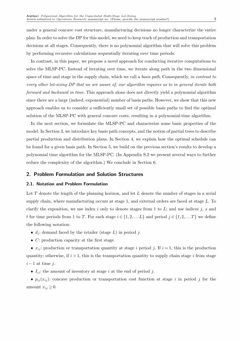
minimum concave cost network flow problem (as in van Hoesel et al. (2005)). Figure 1 illustrates
a network representation of a 10-period problem with 3 stages. The node at stage i in period j is
denoted by (i, j), and has an entering arc with production or transportation quantity xij. Given
this network representation of the problem, a production and distribution plan is a distribution of
the d[1,10] units from the manufacturer’s nodes (1, j) via intermediate nodes (i, j),1< i<L, and to
the retailer’s nodes (L, j).

Author: Polynomial Algorithm for the Capacitated Multi-Stage Lot-SizingArticle submitted to Operations Research; manuscript no. (Please, provide the mansucript number!) 5
x1,1 x1,2 x1,3 x1,4 x1,5 x1,6 x1,8x1,7 x1,9 x1,10
x2,1 x2,2 x2,3 x2,4 x2,5 x2,6 x2,8x2,7 x2,9 x2,10
d[1,10]
d1 d2 d3 d4 d5 d6 d7 d8 d9 d10
x3,1
x3,2
2
x3,3 x3,4 x3,5 x3,6 x3,8x3,7 x3,9 x3,10
Figure 1 The network of production and transportation with inventory
x1,1 x1,2 x1,4 x1,6 x1,8
x2,1 x2,3 x2,4 x2,5 x2,7 x2,9
d[1,10]
d1 d2 d3 d4 d5 d6 d7 d8 d9 d10
x3,1 x3,4 x3,6 x3,8 x3,10
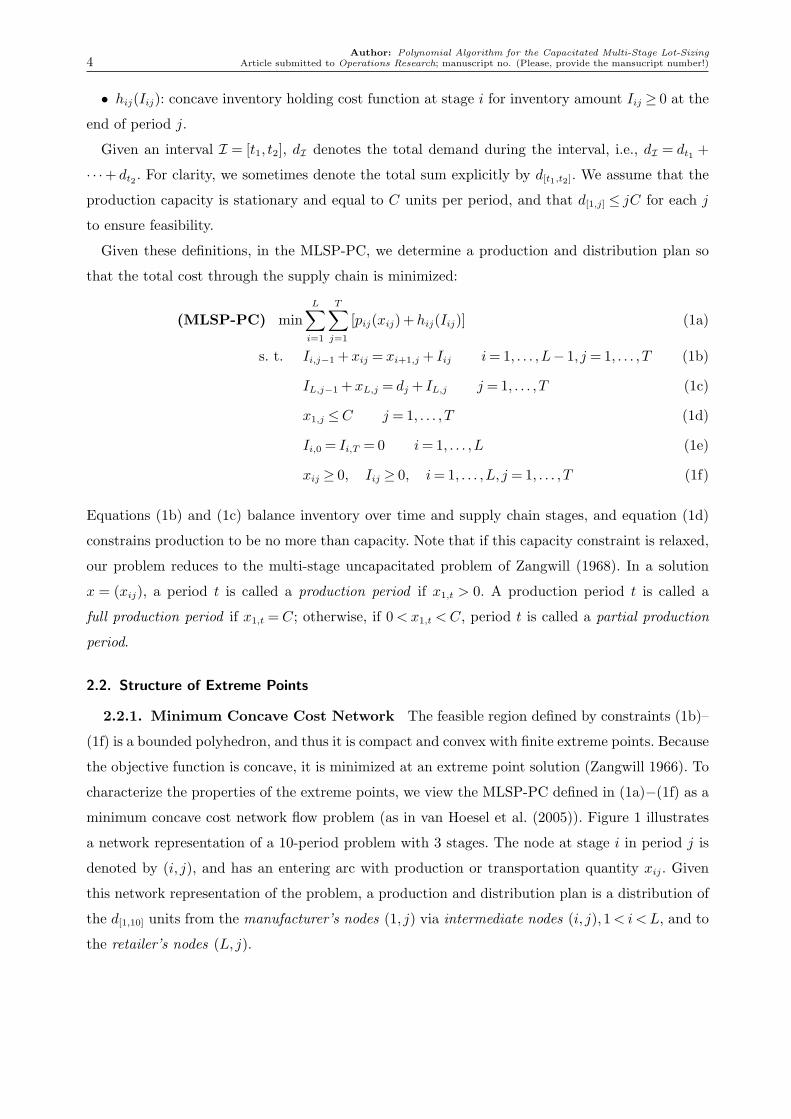
Figure 2 Network flows of a typical extreme point solution
Figure 2 illustrates an extreme point solution of the MLSP-PC. In this figure, each shaded node,
(1, j), represents a period with full production, and each crosshatched node represents a period
with partial production. For instance, in periods 2, 6 and 8 production is at capacity, while in
periods 1 and 4 production is less than capacity but greater than zero. Notice that this network
contains a cycle; for instance, the flows of x1,2, I1,2, x2,3, I2,3, x2,4 and x1,4 make a cycle.
It can be shown that the subnetwork involving only free (or unsaturated) flows of an extreme
point solution contains no cycle (Zangwill 1968; Ahuja et al. 1993) where a flow of production,
transportation or inventory is a free flow if it is strictly between its lower and upper bounds. Since
transportation and inventory quantities have no upper bound, any one of these quantities greater
than zero yield a free flow. The production quantity, however, has upper bound C; consequently,
only partial production yields a free flow. Figure 3 gives the subnetwork of free flows only.
Observe that the subnetwork in Figure 3 has no cycles. In order to focus on critical features of a
minimum concave cost network flow problem, we disregard the flows corresponding to productions
x1,j in the first stage and the flows corresponding to demands. This results in a reduced subnetwork
of an extreme point solution (See Figure ??).

Author: Polynomial Algorithm for the Capacitated Multi-Stage Lot-Sizing6 Article submitted to Operations Research; manuscript no. (Please, provide the mansucript number!)
x1,1 x1,2 x1,4 x1,6 x1,8
x2,1 x2,3 x2,4 x2,5 x2,7 x2,9
d[1,10]
d1 d2 d3 d4 d5 d6 d7 d8 d9 d10
x3,1 x3,4 x3,6 x3,8 x3,10
Figure 3 Network of free flows
2.2.2. Regeneration Network Each connected component of the reduced subnetwork is
called a regeneration network, analogous to a regeneration interval in single-stage capacitated lot-
sizing problems. A production and distribution plan can be described by a set of regeneration
networks. Given a plan, we identify regeneration networks by the earliest and latest periods in
the manufacturer’s and retailer’s stages. In particular, N = (s1, s2, t1, t2) identifies a regeneration
network with the manufacturer’s interval [s1, s2] and the retailer’s interval [t1, t2] where s1 and
s2 are the earliest and latest periods of the network in the manufacturer’s horizon, and t1 and
t2 are the earliest and latest periods of the network in the retailer’s horizon. In Figure ??, there
are two regeneration networks (1,1,1,3) and (2,9,4,10). Note that for any regeneration network
(s1, s2, t1, t2), by definition, we have 1 ≤ s1 ≤ s2 ≤ T , 1 ≤ t1 ≤ t2 ≤ T , s1 ≤ t1 and s2 ≤ t2. Nodes
between two consecutive regeneration networks, N and N ′, do not have any flows associated with
them. We adopt the convention that any node between two regeneration networks belong to the
earlier of the two networks. That is, given two networks N = (s1, s2, t1, t2) and N ′ = (s′1, s′2, t
′1, t
′2),
we extend N to include the nodes (1, s2 + 1), . . . , (1, s′1 − 1) and (L, t2 + 1), . . . , (L, t′1 − 1) so that
we assume s2 = s′1 − 1 and t2 = t′1 − 1.
As mentioned in Subsection 1.2 (based on the results of Zangwill (1968) and Ahuja et al. (1993)),
the network of free flows for the extreme point solution has no cycles. Because a regeneration
network of the extreme point solution is a component of the reduced subnetwork from the network
of free flows, we can see that the regeneration network also contains no cycle. If the regeneration
network has more than one partial production periods, then the original network of free flows will
contain a cycle, which means that the corresponding solution is not an extreme point solution.
Thus, there must be an optimal extreme point solution that has at most one partial production,
or more formally:
Proposition 1. For the MLSP-PC, there exists an (extreme point) optimal solution such that
each regeneration network has no cycle and contains at most one partial production.

Author: Polynomial Algorithm for the Capacitated Multi-Stage Lot-SizingArticle submitted to Operations Research; manuscript no. (Please, provide the mansucript number!) 7
From now on, we consider only the solutions satisfying Proposition 1 and we assume that each
regeneration network is derived from an extreme point solution. Consider a regeneration network N
with retailer’s interval I = [t1, t2]. The assumption of stationary capacity C, together with Propo-
sition 1, reduces the possible choices of production quantity in each period in a given regeneration
network: It should be either zero, or the full production quantity C, or the partial production
quantity, denoted ϵI . Because the network N has at most one partial production, it follows that
the total production quantity should be kC+ ϵI for some nonnegative integer k, which is allocated
to the total amount dI of demand. Hence we have ϵI = dI − ⌊dI/C⌋C. To sum up, a production
quantity of a regeneration network with retailer’s interval I should be one of 0, ϵI ,C where
ϵI = dI −⌊dI/C⌋C.
The DP algorithms in Sections 4 and 5 use state variables representing cumulative production
quantities. In preparation, it is helpful to identify possible cumulative production quantities. Let
ΩI be the set of all possible cumulative production quantities of a regeneration network with the
retailer’s interval I:
ΩI = kC : 0≤ k≤ ⌊dI/C⌋∪ ϵI + kC : 0≤ k≤ ⌊dI/C⌋
Note that the number of elements in the set |ΩI |=O(T ).
2.3. The Dynamic Programming Algorithm for the General MLSP-PC
Let F (s, t) be the cost of the minimum cost solution satisfying demands d1, d2, . . . , dt using pro-
duction in periods 1,2, ..., s in the manufacturer’s horizon. Then, as in van Hoessel (2005), the
following recursion can be used to determine an optimal solution: For 1≤ s2 ≤ t2 ≤ T ,
F (0,0) = 0, and
F (s2, t2) = min1≤s1≤s2,1≤t1≤t2
F (s1 − 1, t1 − 1)+ f(N ) :N = (s1, s2, t1, t2) (2)
where the optimal solution is F (T,T ). If we could compute the minimum cost f(N ) of each
regeneration network N = (s1, s2, t1, t2), we could solve the MLSP-PC using the usual dynamic
programming approach. Of course, this assumes that we are given the cost of each regeneration
network f(N ). Until this paper, however, no polynomial algorithm for computing this cost has
been presented.
3. Basis Path, State and Partial Trees
As we discussed at the start of this paper, all DPs that model multi-period lot-sizing problems
require iterative computation, typically over time. For instance, to solve the single-stage capac-
itated problem defined in Florian and Klein (1971), one needs to solve the optimality equation

Author: Polynomial Algorithm for the Capacitated Multi-Stage Lot-Sizing8 Article submitted to Operations Research; manuscript no. (Please, provide the mansucript number!)
for each state (that is, cumulative production quantity) in a given period, and then repeat these
computations for each subsequent period in order to determine the optimal policy and resulting
plan.
Even for our problem, it is possible to obtain the minimum cost of a regeneration network N ,
f(N ), using the same approach (i.e., iterating over time period). However, as observed by van
Hoesel et al. (2005), this approach cannot solve the problem in polynomial time, as the number
of states that needs to be considered is exponential. In this paper, we propose a different way to
conduct iterative computations to solve the MLSP-PC. Instead of iterating over time, we develop a
DP-based algorithm to find f(N ) by iteratively solving the DP along a specially selected sequence
of nodes (defined by time index and stage).
Before formally developing our DP approach, we introduce several key concepts in this section.
We present the concept of a basis path and define the state variables of the value function in
Subsection 3.1. In 3.2, we introduce the concept of partial trees, which are used to describe subplans,
and in 3.3, we present the structural relationship between a basis path and partial trees. Subsection
3.4 defines the costs associated with partial trees.
3.1. Basis Path and State
Consider a regeneration network N = (s1, s2, t1, t2) of an extreme point solution (satisfying Propo-
sition 1). Because it has no cycle, it is a tree, so there is a unique undirected path between any two
nodes. In this context, a path from a node v1 to another node vk in N is a sequence of distinct
nodes (ir, jr) such that consecutive nodes (ir, jr) and (ir+1, jr+1) have a flow between them for
r= 1,2, ..., k−1. We are particularly interested in the path between nodes (1, s1) and (1, s2) in the
first stage, which we call the basis path of the regeneration network. We call each element of a basis
path a basis node, and note that a basis path coincides with the traditional regeneration interval
in the single-stage capacitated problems.
For a given basis path P = v1, . . . , vk of the regeneration network N , the DP evaluates pro-
duction or transportation decisions for a state at a basis node and then moves to the next basis
node. A state at a basis node vr is represented by a triple (s,ns, t), where ns represents the total
production quantity during the interval [s+ 1, s2] at the manufacturer, and t+ 1 is the starting
time of an interval [t+1, t2] of the retailer’s demands. We call the quantity ns the projected cumu-
lative production quantity (after period s) and the interval [t+1, t2] of demands the projected set of
demands. The information, (s,ns, t) is sufficient to construct the production and distribution plan
for the ns units from the basis node vr, provided that subplans with respect to the basis nodes
vr+1, vr+2, . . ., vk (that is, the nodes on the basis path following vr) are preprocessed. Subsequently,
we will describe how we can characterize all subplans using partial trees.

Author: Polynomial Algorithm for the Capacitated Multi-Stage Lot-SizingArticle submitted to Operations Research; manuscript no. (Please, provide the mansucript number!) 9
1 2 3 4 5 6 7 8 9 10
1
2
3
Figure 4 The basis path for regeneration network (2,9,4,10).
1 2 3 4 5 6 7 8 9 10
1
2
3
Figure 5 The regeneration network and its basis path for non-speculative costs.
Figure 4 shows the basis path (1,2), (1,3), (2,3), . . . , (1,9) of the regeneration network
(2,9,4,10). Observe that the basis path is not sequential in time. For instance, the nodes from
(1,2) to (2,8) are in temporal order, but nodes (2,8) and (2,7) are not. In general, any DP, if it
makes multi-period decisions along a basis path, might move from a state to another state with or
against the time index.
An example of a regeneration network with “non-speculative” cost structure is given in Figure
5. Figures 4 and 5 highlight the differences between the MLSP-PC with general concave costs and
the MLSP-PC with non-speculative costs. For the non-speculative cost structure, the basis path is
explicitly ordered in time: P = (1, s1), (1, s1 + 1), . . . , (1, s2), and this is what allows van Hoesel
et al. (2005) to solve the MLSP-PC by enumerating over the periods associated with the manu-
facturer’s decision. However, with general concave cost structures, the manufacturer’s decisions do
not characterize the optimal policy.
We note that our approach is different from the shortest path network approach of Florian and
Klein (1971). They construct a layered network along time periods in which each node corresponds
to a cumulative production quantity, and the arcs between nodes represent different production
decisions. The optimal production plan corresponds to the shortest path in this network. The basis
path concept we introduce in this paper is significantly different from the shortest path on Florian
and Klein’s network. The basis path is a sequence of nodes (of time and stage) whereas the shortest
path is a sequence of states.
Let fN (P) be the minimum cost for a given basis path P. Then, the cost f(N ) of the regeneration
network is determined by solving the following problem.

Author: Polynomial Algorithm for the Capacitated Multi-Stage Lot-Sizing10 Article submitted to Operations Research; manuscript no. (Please, provide the mansucript number!)
f(N ) =minP
fN (P). (3)
To find an optimal solution for the regeneration network N , we first find an extreme-point
solution that achieves the minimum cost for each basis path P. Then, to determine the optimal
solution for the regeneration network N , the optimal algorithm needs to determine which basis
path is optimal and then the state of each node along the optimal basis path. In the single stage
problem CLSP, the basis path is the same as the regeneration interval, so it suffices to determine
production quantities. Unfortunately, in the multi-stage problem, the basis path is more involved.
As mentioned above, this approach alone does not immediately lead to a polynomial time algo-
rithm (because the number of basis paths is exponential in T and L). However, by utilizing the
structure of the regeneration network - specifically, each node has no more than four neighbors -
we determine the cost at each basis node associated with neighboring basis nodes. This allows us
to significantly reduce the number of paths to be considered, resulting in a polynomial algorithm.
In the next section, we present our algorithm to find the minimum cost for a given basis path,
fN (P), and explain how decisions along the basis path fully determine the complete production
and distribution plan. First, we present preliminary results and definitions.
3.2. Partial Trees
A path from (i1, j1) to (ik, jk) is called a manufacturer-retailer path if the first node (i1, j1) is a
manufacturer’s node and the final node (ik, jk) is a retailer’s node (i.e., i1 = 1 and ik = L). In a
given regeneration network, any partial tree (or subtree) containing a manufacturer-retailer path
is called a comprehensive tree and the partial trees that have no manufacturer-retailer path are
called non-comprehensive trees.
Figure 4 illustrates these definitions. The subtree consisting of nodes (1,2), (1,3) and (2,3) is a
non-comprehensive tree, but the expanded subtree with nodes (1,2), (1,3), (2,3), (2,4) and (3,4)
is a comprehensive tree. If we remove the basis path from the regeneration network (2,9,4,10)
in Figure 4, the remaining components are all non-comprehensive trees, which we specifically
call dangling trees with respect to the basis path. The dangling trees above and below the basis
path are referred to as upper and lower dangling trees, respectively. Our algorithm will carry out
computations along the basis path, incorporating the costs associated with dangling trees along
the way.
Given a node v= (i, j), it is convenient to identify its neighborhood nodes to the north, south, east,
and west of the node v: (i−1, j), (i+1, j), (i, j+1), and (i, j−1). We define B(v) = (i−1, j), (i+
1, j), (i, j+1), (i, j−1) to be the set of neighborhood nodes of (i, j). For notational consistency, we

Author: Polynomial Algorithm for the Capacitated Multi-Stage Lot-SizingArticle submitted to Operations Research; manuscript no. (Please, provide the mansucript number!) 11
2 3 4 5 6
2,4(3,4)
2,4(2,3)
2,4(1,4)
6 7 8 9 10
2,8(3,8)
2,8(2,7)
(a) (b)
Figure 6 Trees around node (2,4) and node (2,8).
add dummy nodes (0, j), (L+1, j), (i,0) and (i, T +1) for 1≤ i≤L and 1≤ j ≤L so that any node
(i, j) always has four neighbors. Consider the connected component of N , which includes the basis
path, in which every node has flows into/out of other nodes. Because the regeneration network Nis a tree (since N has no cycle), cutting any arc of flow divides the component into two parts. For
instance, if we remove the arc of a flow between nodes (i, j) and (i−1, j), the regeneration network
is divided into two subtrees. One of them, which includes the north node (i− 1, j), is denoted by
Tij(i−1, j). In a similar way, we define the south, east, and west trees Tij(i+1, j),Tij(i, j+1), and
Tij(i, j− 1), respectively.
Figure 6(a) shows subtrees of node (2,4) in the regeneration network described in Figure 4,
which are generated by cutting the arcs of flow around (2,4). Because there is no flow to the east
of node (2,4), i.e., from node (2,4) into node (2,5), we say that the east tree is empty. Note that
trees T2,4(3,4) and T2,4(2,3) are non-comprehensive trees whereas T2,4(1,4) is a comprehensive tree.
Figure 6(b) shows comprehensive trees T2,8(2,7) on the west and T2,8(3,8) on the south of node
(2,8) where the north and east trees are empty. Figure 6 also shows that node (2,4) has only one
comprehensive tree around it while node (2,8) has two comprehensive trees.
When determining fN (P) and subsequently solving the problem defined in equation (3), the cost
associated with each transition (from the current state at node vr to the next state at node vr+1)
depends on the location of dangling trees around the current basis node. In addition to the fact
that upper (lower) dangling trees are located above (below) the basis path, we need more precise
information about the location (north, south, east, or west) of dangling trees in order to determine
the associated production/ transportation and inventory costs. To this end, we next explore the
relationship among basis nodes, comprehensive trees, and dangling trees.
3.3. Structure of Partial Trees around a Basis Node
Although there are many possible basis paths connecting the two nodes v1 = (1, s1) and vk = (1, s2)
in the manufacturer’s stage of the regeneration network N = (s1, s2, t1, t2), we can restrict our

Author: Polynomial Algorithm for the Capacitated Multi-Stage Lot-Sizing12 Article submitted to Operations Research; manuscript no. (Please, provide the mansucript number!)
attention to special cases by utilizing the property thatN contains no cycles. We begin by bounding
the number of comprehensive trees around each basis node. For this, we use the no-cycle property
(Proposition 1) and the fact that a comprehensive tree always contains a manufacturer-retailer
path (from the definition).
Proposition 2. Given a node v on a regeneration network, there are at most two comprehensive
trees among the four trees Tv(u), u∈B(v).
For each basis node vr in the basis path P = v1, . . . , vk, we call nodes vr−1 and vr+1 the
previous node and subsequent node of vr, respectively. For notational convenience, we assume that
the first node v1 has as its previous node v0 = (1, s1 − 1) and the last node vk has its subsequent
node vk+1 = (1, s2 + 1). In the same manner, we call Tvr(vr−1) and Tvr(vr+1) the previous and
subsequent trees of basis node vr. We note that the previous tree contains nodes v1, v2, . . . , vr−1 and
the subsequent tree contains nodes vr+1, vr+2, . . . , vk and we also notice that all subsequent trees
are comprehensive. To see this, first consider the subsequent tree Tvk−1(vk) of node vk−1. Because
node vk, i.e., the manufacturer’s last node (1, s2), has a path to the retailer’s last node (L, t2),
we see that the tree Tvk−1(vk) is a comprehensive tree. Then, any subsequent tree Tvr(vr+1) of
basis node vr, r < k, contains the node vk and hence it has a manufacturer-retailer path from vk
to (L, t2), implying that it must be a comprehensive tree. However, previous trees are not always
comprehensive trees. For example, the previous tree Tv2(v1) of node v2 is not comprehensive.
For given previous and subsequent nodes, vr−1 and vr+1, we can determine the locations and
(either upper or lower) types of dangling trees around a basis node vr. To see this, suppose that
the subsequent node is north of vr, i.e., vr+1 = (i− 1, j). Then, the previous node will be one of
(i, j + 1), (i + 1, j) and (i, j − 1). The three possible cases for the location of the previous tree
when vr+1 = (i − 1, j) are illustrated in Figure 7(a). The possible cases when vr+1 = (i, j + 1)
are illustrated in Figure 7(b). Note that when the subsequent node lies to the south of node vr
(i.e., vr = (i+ 1, j)), there are only two possible locations for the previous node as only acyclic
subnetworks are permitted. Specifically, the previous node cannot be the east node (i, j+1) since
we cannot have the east comprehensive tree Tij(i, j + 1) preceding the south comprehensive tree
Tij(i+1, j) without creating a cycle. Likewise, when vr+1 = (i, j− 1), the previous node cannot be
the the north node (i−1, j) (see Figures 7(c) and (d), respectively). Figure 7 illustrates all possible
(ten) cases. Note that there can be at most two dangling trees at any basis node. Also note that
their locations (that is, their directions) are determined once the previous and subsequent trees
are identified. For instance, if the three consecutive basis nodes are vr−1 = (i+ 1, j), vr = (i, j),
vr+1 = (i− 1, j), there can be an upper dangling tree on the west and/or a lower dangling tree on

Author: Polynomial Algorithm for the Capacitated Multi-Stage Lot-SizingArticle submitted to Operations Research; manuscript no. (Please, provide the mansucript number!) 13
ij
ij
ij
(i 1, j), (i, j), (i 1, j)(i, j 1), (i, j), (i 1, j) (i, j 1), (i, j), (i 1, j)
(a1) (a2) (a3)
(a) Subsequent comprehensive trees in the north
(i, j 1), (i, j), (i, j 1)(i 1, j), (i, j), (i, j 1)(i 1, j), (i, j), (i, j 1)
ij
ijij
(b1) (b2) (b3)
(b) Subsequent comprehensive trees in the east
ij
(i, j 1), (i, j), (i 1, j)
ij
ij
(i, j 1), (i, j), (i, j 1)(i 1, j), (i, j), (i 1, j)
ij
(c1) (c2)
(c) Subsequent comprehensive trees in the south
(d1) (d2)
(d) Subsequent comprehensive trees in the west
(i 1, j), (i, j), (i, j 1)
Figure 7 Possible forms of comprehensive trees around (i, j).
the east (Figure 7(a2)). If the three nodes are (i+1), (i, j), and (i, j+1), only upper dangling trees
can exist (at the north and west of node (i, j)).
Before closing this subsection, it is worth emphasizing the relationship between the state (s,ns, t)
at the current basis node, vr and the subsequent tree, Tvr(vr+1). A state (s,ns, t) of basis node vr
implies a minimum-cost subsequent tree containing the basis nodes vr+1, vr+2, . . ., vk. As a result,
Tvr(vr+1) has the manufacturer’s nodes for periods s + 1 through s2 during which ns units are
produced and allocated for demands dt+1, dt+2, . . ., dt2 .
3.4. Costs of Dangling Trees
For upper dangling trees, we define φ(i, j)a,s′,s to be the minimum cost to produce a ∈ ΩI units
during [s′, s] in the manufacturer’s horizon and then to transport/inventory these units to inter-
mediate node (i, j), s′ ≤ s≤ j, 1≤ i≤L. If s′ > s, we set φ(i, j)a,s′,s = 0. If a basis node (i, j) lies in
the manufacturer’s horizon, i.e., i= 1, it has no upper dangling trees. For convenience, we define a
virtual upper tree T1,j(0, j) of node (1, j) so we can consistently use the term φ(i, j)a,s′,s; we define
φ(0, j)a,s′,s = 0 for any arguments a, s′ and s.

Author: Polynomial Algorithm for the Capacitated Multi-Stage Lot-Sizing14 Article submitted to Operations Research; manuscript no. (Please, provide the mansucript number!)
For lower dangling trees, we define ϕ(i, j)t′,t to be the minimum cost of satisfying demands
dt′ , dt′+1, . . . , dt using d[t′,t] units in node (i, j), j ≤ t′ ≤ t. If t′ > t, we set ϕ(i, j)t′,t = 0. We also define
a virtual lower dangling tree, for convenience, for basis nodes in the retailer’s horizon. We define
ϕ(L+1, j)t′,t = 0 for any arguments t′ and t. Given these definitions, the procedure to compute the
costs of upper and lower dangling trees is relatively straightforward because of their arborescent
structures. For completeness, we provide details in Appendix S.1.
4. Planning with Known Basis Path
In this section, we assume that we are given a basis path P over which our algorithm iterates. To
illustrate how our algorithm works, we first start with the single-stage problem CLSP in which each
state can be described by a projected cumulative quantity and then extend it to the multi-stage
problem in which each state needs a projected set of demands as well as a projected cumulative
quantity. We note that the approach for solving the CLSP in the next subsection is substantially
different from Florian and Klein (1971) in the sense that they use as a state the cumulative
production quantity (rather than projected cumulative production quantity).
4.1. Planning with Projected Cumulative Production Quantities
Note that in the CLSP, s1 = t1 and s2 = t2 for any regeneration network N = (s1, s2, t1, t2). That
is, the retailer’s interval, I = [t1, t2] coincides with the production interval, [s1, s2]. As a result,
any regeneration network N has only one basis path (1, s1), . . . , (1, s2), which is a regeneration
interval in the usual sense.
For each node (1, s), s ∈ I, the projected cumulative production quantity ns after period s+1
is ns = x1,s+1 + · · ·+ x1,s2 where ns ∈ ΩI . These quantities, ns for s = s1, . . . , s2, are sufficient to
compute the detailed production plan. We begin by denoting by (s,ns) the state in which we
produce ns units during [s+1, s2] to satisfy demands in [s+1, s2]. In period s, we must determine
the number of units to be produced, which must be one of zero, partial production quantity ϵI , or
full production quantity C (Proposition 1). If the production quantity in period s is a∈ 0, ϵI ,C,
then the state at period s− 1 is described by (s− 1, a+ns) where a+ns ∈ΩI .
To compute the cost of regeneration network N , let fN (s)ns be the minimum cost of satisfying
the demands in the interval [s1, s]⊆ I when the projected cumulative production quantity is ns.
(We note that the state of projected cumulative production appears in superscript. We will also
follow this convention when dealing with the multi-stage problem.)
Here, the quantity ns is not arbitrary but is instead one of the values in ΩI (and indeed, this
is what makes the problem polynomially solvable). Note that the cost f(N ) of the regeneration
network is equal to fN (s2)0. To obtain fN (s)ns , in general we only need to determine the production

Author: Polynomial Algorithm for the Capacitated Multi-Stage Lot-SizingArticle submitted to Operations Research; manuscript no. (Please, provide the mansucript number!) 15
quantity a in period s. Because period s2 is a regeneration period such that I1,s2 = 0, the cumulative
production quantity from period s through s2 is not larger than the total sum of demands d[s,s2],
i.e., a+ns ≤ d[s,s2]. Then, the additional d[s,s2] − a−ns units must be held in inventory at the end
of period s− 1 to meet remaining demand that production during [s, s2] could not supply for the
demands ds, . . . , ds2 . Let cI(s)a,s,ns be the immediate cost at the current node (1, s) which consists
of two components: the production cost in period s, and the cost of carrying the inventory at the
end of period s− 1, i.e.,
cI(s)a,s,ns = h1,s−1(d[s,s2] − a−ns)+ p1,s(a).
The cost cI(s)a,s,ns at node (1, s) is in fact the cost from changing state (s− 1, a+ ns) to state
(s,ns). With the immediate costs, we can compute the minimum cost fN (s)ns using the following
optimality equation:
fN (s)ns =mina
fN (s− 1)a+ns + cI(s)a,s,ns : a+ns ∈ΩI, (4)
with initial condition fN (s0)dI = 0 and s0 = s1−1. We note that the initial condition of the formula
(fN (s0)dI = 0) means that the projected cumulative quantity is just the total sum of demands
which is to be produced after period s0 and hence there is nothing to be done at period s0.
4.2. Immediate Cost at a Basis Node for the MLSP-PC
The recursive formula (4) demonstrates that the single-stage problem is solved by a forward algo-
rithm in time periods. We solve the multi-stage problem using a similar approach. However, in
contrast to the single-stage problem in which each basis path is the regeneration interval itself,
the regeneration network in the multi-stage problem has basis paths that are not ordered in time
period. We will evaluate the cost fN (P) of an optimal policy for a given regeneration network
with the basis path P = v1, v2, . . . , vk by extending the value function fN (s)ns for the single
stage problem (CLSP) to the multi-stage problem (MLSP-PC). To do this, we need to define the
immediate cost at a basis node vr.
For a regeneration network N with retailer’s interval I = [t1, t2], consider a basis node vr with its
state (s,ns, t) and its previous and subsequent nodes vr−1 and vr+1. By construction, the subsequent
tree Tvr(vr+1) contains manufacturer’s nodes s+ 1 through s2 producing ns units, and retailer’s
nodes t+1 through t2. Suppose that node vr has upper dangling trees containing manufacturer’s
periods s′+1 through s and lower dangling trees containing retailer’s periods t′+1 through t where
s1 ≤ s′ ≤ s≤ s2 and t1 ≤ t′ ≤ t≤ t2. Let a be the total production quantity during [s′ +1, s] of the
upper dangling trees. Then we define the immediate cost as follows:

Author: Polynomial Algorithm for the Capacitated Multi-Stage Lot-Sizing16 Article submitted to Operations Research; manuscript no. (Please, provide the mansucript number!)
Definition 1. The immediate cost at basis node vr, denoted by cI(vr−1, vr, vr+1)s′,a,s,nst′,t , is the
minimum cost associated with the flows between vr and vr−1, the flows from all upper dangling
trees into vr, and the flows from vr to all lower dangling trees.
Note that the immediate cost at a basis node vr includes all costs associated with dangling trees
and the flows around node vr except for the cost of the flow between nodes vr and vr+1 (i.e. the cost
of the flow between the current and subsequent nodes), which is considered when the immediate
cost at basis node vr+1 is determined.
The precise functional form of the immediate cost depends on the types of dangling trees and
their locations (i.e., the ten cases listed in Figure 8). Since a basis node can have at most two
dangling trees, a number of possibilities exist: both trees are upper dangling trees, both trees are
lower dangling trees, one of them is an upper dangling tree and the other one is a lower dangling
tree, or there is only one (or no) dangling tree (see Figure 8). Any case with one or no dangling
tree is a special case of two dangling trees.
When determining cI(vr−1, vr, vr+1)s′,a,s,nst′,t (we abbreviate this to cI(·) where the meaning is
obvious), we note that we only need information about the retailer’s interval I = [t1, t2], not the
full information about a regeneration network N = (s1, s2, t1, t2). This is because the (partial)
production quantity depends only on retailer’s interval I. In other words, the quantity a in the
cost cI(vr−1, vr, vr+1)s′,a,s,nst′,t should be one of 0, ϵI ,C.
In this section, we explain how to determine the immediate costs for two representative cases.
The first case has one upper dangling tree and one lower dangling tree, with three consecutive
basis nodes (i+1, j), (i, j) and (i− 1, j). The second case has two upper dangling trees with three
consecutive basis nodes (i+ 1, j) (i, j) and (i, j + 1). (Figure 7). All remaining cases (there are
10 cases as shown in Figure 7) can be analyzed in a similar manner. Later we will show that the
second case where vr has two upper dangling trees is the most computationally demanding, and
thus it determines the complexity of algorithm.
In computing the immediate cost, we assume that the subsequent tree Tvr(vr+1) produces ns
units during periods [s+1, s2] to supply demands dt+1, . . . , dt2 . In other words, Tvr(vr+1) contains
manufacturer’s nodes of periods [s+1, s2] with cumulative projected production quantity ns, and
retailer’s nodes of periods [t+1, t2] for projected set of demands.
4.2.1. Case 1: vr−1 = (i+ 1, j), vr = (i, j), vr+1 = (i− 1, j) For this case, we have previous
and subsequent trees Tij(i+1, j) and Tij(i− 1, j), respectively, and possibly (non-empty) dangling
trees around node (i, j): an upper dangling tree Tij(i, j− 1) and a lower dangling tree Tij(i, j+1)
(see Figure 7(a2) and 8). The upper dangling tree Tij(i, j − 1) contains the manufacturer’s nodes
for periods s′ +1 through s for some s′, s1 ≤ s′ ≤ s, during which, say, a units are produced. Note

Author: Polynomial Algorithm for the Capacitated Multi-Stage Lot-SizingArticle submitted to Operations Research; manuscript no. (Please, provide the mansucript number!) 17
[ 1, ]
units
s s
a
! 2[ 1, ]
unitss
s s
n
1 2
1
,
[ , ]
( ) unitst t s
s s
d a n
! "
2[ 1, ]t t [ 1, ]t t !1[ , ]t t
ij
Figure 8 Partial trees for consecutive basis nodes (i− 1, j), (i, j), (i+1, j)
,
[ 1, ]
units
s s
a b
!
"
2[ 1, ]
unitss
s s
n
1 2
1
,
[ , ]
( ) unitst t s
s s
d a n
! "
2[ 1, ]t t 1[ , ]t t
[ 1, ]
units
s s
b
!
ij
Figure 9 Partial trees for consecutive basis nodes (i+1, j), (i, j), (i, j+1)
that if s′ = s, the upper dangling tree is empty. Likewise, the lower dangling tree contains retailer’s
nodes for periods t′ + 1 through t for t1 ≤ t′ ≤ t. Again, if t′ = t, then the lower dangling tree is
empty.
The a units produced in the upper dangling tree Tij(i, j− 1) result in a cost of φ(i, j− 1)a,s′+1,s,
plus an additional holding cost hi,j−1(a) to carry inventory from period j − 1 to period j in the
warehouse at stage i. For the lower dangling tree, the cost is ϕ(i, j+1)t′+1,t of satisfying demands in
[t′+1, t], for which d[t′+1,t] units are carried over from period j in the warehouse at stage i incurring
holding cost hij(d[t′+1,t]). Hence the total cost of the dangling trees is ϕ(i, j+1)t′+1,t+hij(d[t′+1,t])+
φ(i, j − 1)a,s′+1,s + hi,j−1(a). Finally, we consider the cost associated with the flow between node
(i, j) and node (i+ 1, j). The total cumulative production quantity during [s′ + 1, s2] (combining
the production of the upper dangling tree Tij(i, j − 1) and the subsequent tree Tij(i − 1, j)) is
a + ns. After meeting demand in [t′ + 1, t2], the remaining a + ns − d[t′+1,t2] ≥ 0 units at node
(i, j) are transported from stage i warehouse to stage i+ 1 warehouse with transportation cost
pi+1,j(a+ns − d[t′+1,t2]). Thus, the total immediate cost at the basis node (i, j) for this case is:
cI(vr−1, vr, vr+1)s′,a,s,nst′,t = pi+1,j(a+ns − d[t′+1,t2])+ϕ(i, j+1)t′+1,t +hij(d[t′+1,t])
+φ(i, j− 1)a,s′+1,s +hi,j−1(a).

Author: Polynomial Algorithm for the Capacitated Multi-Stage Lot-Sizing18 Article submitted to Operations Research; manuscript no. (Please, provide the mansucript number!)
4.2.2. Case 2: vr−1 = (i + 1, j), vr = (i, j), vr+1 = (i, j + 1) If the three consecutive nodes
(i+1, j), (i, j) and (i, j+1) are on the basis path, there may be two upper dangling trees, Tij(i, j−1)
and Tij(i− 1, j), but there will be no lower dangling tree (see Figure 7(b2) and Figure 9). Assume
that the north dangling tree has manufacturer’s nodes for periods s′′+1 to s and the west dangling
tree has nodes for periods s′+1 to s′′. Suppose that a∈ΩI units are produced during [s′+1, s] in
the two upper dangling trees and b∈ΩI units are produced in the north dangling tree Tij(i− 1, j)
in periods [s′′ + 1, s]; hence a− b ∈ ΩI units are produced at the west upper dangling tree. The
cost of producing b units in the north dangling tree and transporting them to node (i, j) is φ(i−
1, j)b,s′′+1,s + pij(b), and the cost of producing a− b units in the west dangling tree and carrying
them over to node (i, j) is φ(i, j−1)a−b,s′+1,s′′ +hi,j−1(a−b). Finally note that the total production
quantity from period s′ +1 to s2 is a+ns, some of which meets demand from periods t+1 to t2.
The remaining a+ ns − d[t+1,t2] ≥ 0 units are transported from node (i, j) to node (i+ 1, j) (see
Figure 9), incurring cost pi+1,j(a+ns−d[t+1,t2]). Therefore the total cost at the basis node (i, j) in
this case is:
pi+1,j(a+ns − d[t+1,t2])+φ(i, j− 1)a−b,s′+1,s′′ +hi,j−1(a− b)+φ(i− 1, j)b,s′′+1,s + pij(b).
We now determine the immediate cost, cI(·). Accounting for the quantity (and the cost) associ-
ated with each upper dangling tree (by enumerating production in the north dangling tree, denoted
by b), the immediate cost at the basis node (i, j) is given as:
cI(vr−1, vr, vr+1)s′,a,s,nst′,t = min
b∈ΩI ,s′≤s′′≤s
pi+1,j(a+ns − d[t+1,t2])+φ(i, j− 1)a−b,s′+1,s′′
+hi,j−1(a− b)+φ(i− 1, j)b,s′′+1,s + pij(b)
.
Following the logic developed in the two previous subsections, we can compute the immediate
costs for all of the ten cases in Figure 7 (see Table 1). To clarify which parameters (and information)
are necessary to compute cI(·), we omit unnecessary arguments in the third column of Table 1.
For example, when vr−1 = (i− 1, j), vr = (i, j) and vr+1 = (i+ 1, j), we do not have any dangling
trees (the dangling trees are all empty). In this case, if our current state is (s,ns, t) at node vr, we
have s′ = s, a= 0 and t′ = t in cI(vr−1, vr, vr+1)s′,a,s,nst′,t . Omitting the (trivial) terms s′ and a when
the upper dangling tree is empty (or the t′ when the lower dangling tree is empty) clarifies the
presentation.
We now analyze the computational complexity of determining costs cI(vr−1, vr, vr+1)s′,a,s,nst′,t for
a given regeneration network with retailer’s time interval I. First, note that the number of cases
of consecutive basis nodes (vr−1, vr and vr+1) is O(LT ). This is because the number of nodes vr
is O(LT ) and because any node vr will have its previous (subsequent) node vr−1 (vr+1) as one
of the four components of B(vr). We now focus on the complexity of computing the immediate

Author: Polynomial Algorithm for the Capacitated Multi-Stage Lot-SizingArticle submitted to Operations Research; manuscript no. (Please, provide the mansucript number!) 19
Table 1 Immediate costs at basis nodes.
Basis nodes cost at basis node (i, j) cI(·)s′,a,s,ns
t′,t
(i, j+1), (i, j), (i− 1, j) hij(a+ns − d[t+1,t2])+φ(i, j− 1)a,s′+1,s +hi,j−1(a) cI(·)s
′,a,s,nst
(i+1, j), (i, j), (i− 1, j) pi+1,j(a+ns − d[t′+1,t2])+ϕ(i, j+1)t′+1,t +hij(d[t′+1,t]) cI(·)s′,a,s,ns
t′,t
φ(i, j− 1)a,s′+1,s +hi,j−1(a)
(i, j− 1), (i, j), (i− 1, j) min1hi,j−1(d[t′+1,t2] −ns)+ϕ(i+1, j)t′+1,t′′ + pi+1,j(d[t′+1,t′′]) cI(·)s,nst′,t
+ϕ(i, j+1)t′′+1,t +hi,j(d[t′′+1,t])(i− 1, j), (i, j), (i, j+1) pij(d[t′+1,t2] −ns)+ϕ(i+1, j)t′+1,t + pi+1,j(d[t′+1,t]) cI(·)s,ns
t′,t
(i+1, j), (i, j), (i, j+1) min2pi+1,j(a+ns − d[t+1,t2])+φ(i, j− 1)a−b,s′+1,s′′ cI(·)s′,a,s,ns
t
+hi,j−1(a− b)+φ(i− 1, j)b,s′′+1,s + pij(b)
(i, j− 1), (i, j), (i, j+1) hi,j−1(d[t′+1,t2] − a−ns)+ϕ(i+1, j)t′+1,t + pi+1,j(d[t′+1,t]) cI(·)s′,a,s,ns
t′,t
+φ(i− 1, j)a,s′+1,s + pij(a)
(i− 1, j), (i, j), (i+1, j) pij(d[t+1,t2] −ns) cI(·)s,nst
(i, j− 1), (i, j), (i+1, j) hi,j−1(d[t+1,t2] − a−ns)+φ(i− 1, j)a,s′+1,s + pij(a) cI(·)s
′,a,s,nst
(i, j+1), (i, j), (i, j− 1) hij(ns − d[t+1,t2]) cI(·)s,nst
(i+1, j), (i, j), (i, j− 1) pi+1,j(ns − d[t′+1,t2])+ϕ(i, j+1)t′+1,t +hij(d[t′+1,t]) cI(·)s,nst′,t
min1 is over t′ ≤ t′′ ≤ tmin2 is over b∈ΩI , s
′ ≤ s′′ ≤ s
cost for possible states. The second column of Table 1 presents the immediate costs for all the ten
cases. It shows that only two cases involve a minimum operator: the case with two lower dangling
trees, (vr−1 = (i, j − 1), vr = (i, j), vr+1 = (i − 1, j)) or the case with two upper dangling trees
(vr−1 = (i+ 1, j), vr = (i, j), vr+1 = (i, j + 1)). The remaining 8 cases can be evaluated in constant
time.
To determine the complexity of these 8 cases, first note that the computing time depends on the
number of arguments necessary to determine cI(vr−1, vr, vr+1)s′,a,s,nst′,t . The necessary arguments are
shown in the third column of Table 1. Observe that the two worst cases among these 8 cases are
((i+ 1, j), (i, j), (i− 1, j)) and ((i, j − 1), (i, j), (i, j + 1)): both cases have six arguments: s′, a, s,
ns, t′ and t. Since each of these arguments has O(T ) possible instances, for given (vr−1, vr, vr+1),
the maximum complexity is O(T 6). Since there are O(LT ) basis nodes to be considered, the total
complexity is O(LT 7).
We now consider the two cases that contain a minimum operator. In the case with two upper-
dangling trees, the expression inside the minimum operator has five arguments (O(T 5)). To deter-
mine cI(vr−1, vr, vr+1)s′,a,s,nst′,t , we need to enumerate over b and s′′ (O(T 2)). Hence, it takes O(T 7)
time to determine cI(vr−1, vr, vr+1)s′,a,s,nst′,t for given (vr−1, vr, vr+1). Since there are O(LT ) basis
nodes, we can see that the total computing time for the case with two upper-dangling trees is
O(LT 8). A similar analysis shows that it takes O(LT 6) for the case with two lower-dangling trees.
Comparing the complexities of all ten cases, we conclude that it takes (LT 8) to compute all the
immediate costs for a given regeneration network with retailer’s time interval I. Finally, because
there are O(T 2) intervals I, the total computing time for all regeneration networks is (LT 10).
Appendix S.2 companion contains several ways to further reduce the complexity.
Author: Polynomial Algorithm for the Capacitated Multi-Stage Lot-Sizing20 Article submitted to Operations Research; manuscript no. (Please, provide the mansucript number!)
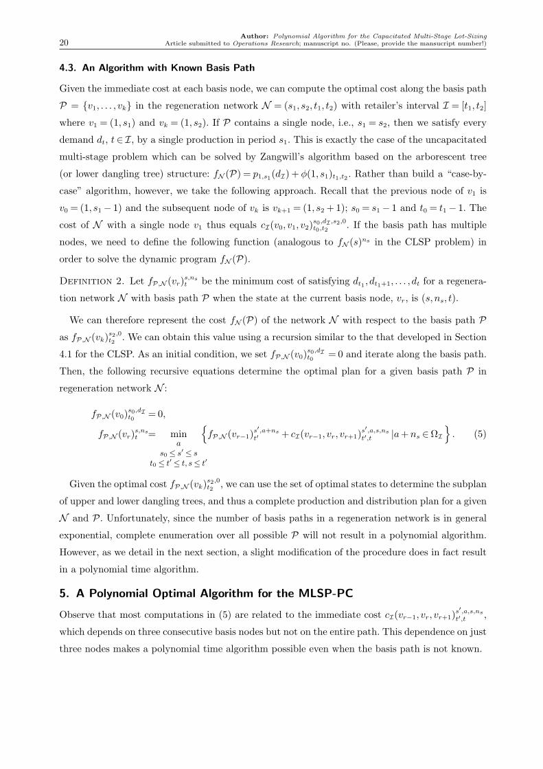
4.3. An Algorithm with Known Basis Path
Given the immediate cost at each basis node, we can compute the optimal cost along the basis path
P = v1, . . . , vk in the regeneration network N = (s1, s2, t1, t2) with retailer’s interval I = [t1, t2]
where v1 = (1, s1) and vk = (1, s2). If P contains a single node, i.e., s1 = s2, then we satisfy every
demand dt, t∈ I, by a single production in period s1. This is exactly the case of the uncapacitated
multi-stage problem which can be solved by Zangwill’s algorithm based on the arborescent tree
(or lower dangling tree) structure: fN (P) = p1,s1(dI) + ϕ(1, s1)t1,t2 . Rather than build a “case-by-
case” algorithm, however, we take the following approach. Recall that the previous node of v1 is
v0 = (1, s1 − 1) and the subsequent node of vk is vk+1 = (1, s2 +1); s0 = s1 − 1 and t0 = t1 − 1. The
cost of N with a single node v1 thus equals cI(v0, v1, v2)s0,dI ,s2,0t0,t2
. If the basis path has multiple
nodes, we need to define the following function (analogous to fN (s)ns in the CLSP problem) in
order to solve the dynamic program fN (P).
Definition 2. Let fP,N (vr)s,nst be the minimum cost of satisfying dt1 , dt1+1, . . . , dt for a regenera-
tion network N with basis path P when the state at the current basis node, vr, is (s,ns, t).
We can therefore represent the cost fN (P) of the network N with respect to the basis path P
as fP,N (vk)s2,0t2
. We can obtain this value using a recursion similar to the that developed in Section
4.1 for the CLSP. As an initial condition, we set fP,N (v0)s0,dIt0
= 0 and iterate along the basis path.
Then, the following recursive equations determine the optimal plan for a given basis path P in
regeneration network N :
fP,N (v0)s0,dIt0
= 0,
fP,N (vr)s,nst = min
as0 ≤ s′ ≤ s
t0 ≤ t′ ≤ t, s≤ t′
fP,N (vr−1)
s′,a+nst′ + cI(vr−1, vr, vr+1)
s′,a,s,nst′,t |a+ns ∈ΩI
. (5)
Given the optimal cost fP,N (vk)s2,0t2
, we can use the set of optimal states to determine the subplan
of upper and lower dangling trees, and thus a complete production and distribution plan for a given
N and P. Unfortunately, since the number of basis paths in a regeneration network is in general
exponential, complete enumeration over all possible P will not result in a polynomial algorithm.
However, as we detail in the next section, a slight modification of the procedure does in fact result
in a polynomial time algorithm.
5. A Polynomial Optimal Algorithm for the MLSP-PC
Observe that most computations in (5) are related to the immediate cost cI(vr−1, vr, vr+1)s′,a,s,nst′,t ,
which depends on three consecutive basis nodes but not on the entire path. This dependence on just
three nodes makes a polynomial time algorithm possible even when the basis path is not known.

Author: Polynomial Algorithm for the Capacitated Multi-Stage Lot-SizingArticle submitted to Operations Research; manuscript no. (Please, provide the mansucript number!) 21
Given a regeneration network N = (s1, s2, t1, t2), we know the first and last nodes of an optimal
basis path; that is, v1 = (1, s1) and vk = (1, s2) for some k. (Note that to be consistent with our
development to this point, we use vk to denote the last node in the basis path.) The intermediate
nodes (between v1 and vk) will be determined dynamically during the iteration of the DP. Because
the basis nodes are determined by the DP, we need to extend the state (the projected quantity
and the projected set of demands) for the previous algorithm with known basis path to include the
current node v and its subsequent node w. Thus, we define a state by (v,w, s,ns, t) that describes
the situation in which v and w are assumed to be consecutive basis nodes (in a basis path) and the
subsequent tree Tv(w) of node v produces ns ∈ ΩI units during [s+1, s2] to meet demand in the
interval [t+1, t2]. Notice that if the current node v and its subsequent node w are known, the DP
must identify the previous node to compute the immediate cost at v. Although we do not explicitly
know its previous node, we know that it belongs to the neighborhood of v, i.e., B(v). Since the
subsequent node also belongs to B(v), the previous node belongs, more precisely to B(v)− w.
For the node v and its subsequent node w, the optimal path from v back to the first node v1 is
obtained recursively by choosing the best neighbor node u ∈B(v)−w. We explicitly define the
value function for the state (v,w, s,ns, t) below:
Definition 3. Let fN (v,w)s,nst be the value function for the state (v,w, s,ns, t); that is, the min-
imum cost of satisfying demands dt1 , dt1+1, . . . , dt if v and w are consecutive basis nodes in a basis
path and the subsequent tree Tv(w) of node v produces ns ∈ ΩI units during [s+ 1, s2] to meet
demand in the interval [t+1, t2].
By this definition, the cost f(N ) of the regeneration network is fN (vk, vk+1)s2,0t2
. For the initial
condition, we set fN (v0, v1)s0,dIt0
= 0. From (5) developed for the case with a known basis path, we
see that if the previous node of v is u, then for a given a, s′, and t′, the total cost is given as follows:
fN (u, v)s′,a+ns
t′ + cI(u, v,w)s′,a,s,nst′,t : a+ns ∈ΩI .
By considering all cases of u∈B(v)−w, we obtain the following optimality equation:
fN (v0, v1)s0,dIt0
= 0,
fN (v,w)s,nst = min
as0 ≤ s′ ≤ s
t0 ≤ t′ ≤ t, s≤ t′
fN (u, v)s
′,a+nst′ + cI(u, v,w)
s′,a,s,nst′,t |a+ns ∈ΩI , u∈B(v)−w
. (6)
By solving this DP, we obtain the optimal policy for each state (v,w, s,ns, t). The policy is
described by, among other things, the sequence of (basis) nodes from the first node v1 to the node
v under consideration. Note that the path of nodes from v1 to v is not unique but depends on the
Author: Polynomial Algorithm for the Capacitated Multi-Stage Lot-Sizing22 Article submitted to Operations Research; manuscript no. (Please, provide the mansucript number!)
subsequent node, the projected cumulative production quantity and the projected set of demands
with the respect to the node v. Given a node v, the subsequent node w is one of the neighbors
in B(v), so that the possible number of the subsequent nodes is four. Because there are O(T 2)
pairs (s,ns) for the projected cumulative production quantity and O(T ) of t for the projected set
of demands, the total number of possible states with respect to node v is O(4T 3). This means that
there can be up to O(T 3) basis paths from v1 to v. Because there are O(LT ) nodes v, the total
number of possible paths constructed during the DP iterations is O(LT 4). That is, the number of
paths is a polynomial function of L and T , which is determined by the size of the state space of
(v,w, s,ns, t).
To evaluate the overall complexity of this DP, first observe that each regeneration network
N = (s1, s2, t1, t2) is specified by four parameters, so O(T 4) regeneration networks are considered.
Given a regeneration network N , for each state (v,w, s,ns, t) we evaluate fN (v,w)s,nst for which we
need additional parameters s′, t′ and the quantity a in the main optimality recursion (6). Hence,
the overall complexity would seem to naively require up to O(LT 11). In Appendix S.2, we detail
how eliminating double counting will reduce the complexity of this algorithm to O(LT 10), and how
taking advantage of the structure of the cost function and consolidating regeneration networks will
further reduce the complexity to O(LT 8).
6. Conclusion
In this paper, we consider a multi-stage lot-sizing problem for a serial supply chain where the
production is capacitated at the first stage. To capture the general economies of scale not only
in production but also in transportation, we assume general concave costs with speculative cost
structure through the entire supply chain. This general problem is significantly different from the
special case disallowing speculative motives in transportation in that the manufacturer’s decision
at the first stage does not uniquely determine transportation decisions at later stages.
This paper presents the first polynomial-time algorithm for this problem (in the length of plan-
ning horizon and the number of stages in the supply chain). To develop this algorithm, we introduce
the concept of a basis path. Traditionally, lot-sizing problems are solved by sequentially iterating
over time periods. However, by instead iterating over the basis path, we are able to sufficiently
reduce the state space of the problem. We believe that this concept of the basis path has the
potential to be applied to other discrete time optimization problems. The model considered in this
paper is limited to a capacity at the first stage. Our solution approach based on a basis path can
be extended to other problems, such as multi-stage lot-sizing problems where mid-level operations
are constrained by capacity (e.g., transportation decisions are constrained, a multi-level extension

Author: Polynomial Algorithm for the Capacitated Multi-Stage Lot-SizingArticle submitted to Operations Research; manuscript no. (Please, provide the mansucript number!) 23
of the two-stage model considered in Lee et al., 2003). We believe that our basis path approach
can be used to solve these and similar problems in polynomial time.
Acknowledgments
This research was supported by Basic Science Research Program through the National Research Foundation
of Korea(NRF) funded by the Ministry of Education, Science and Technology(2010-0021551).
References
Aggarwal, A. and Park, J.K. 1993. Improved algorithms for economic lot-size problems. Operations Research
41, 549–571.
Ahuja, R. K., T. L. Magnanti, J. B. Orlin. 1993. Network Flows: Theory Algorithms, and Applications.
Prentice Hall, CityplaceEnglewood Cliffs, NJ.
Chung, C.S. and Lin, C.H.M. 1988. An O(T 2) algorithm for the NI/G/NI/ND capacitated lot size problem.
Management Science 34 420–426.
Federgruen, A. and Tzur, M. 1991. A simple forward algorithm to solve general dynamic lot-sizing models
with n periods in O(n logn) or O(n) Time. Management Science 37 909–925.
Florian, M. and Klein, M. 1971. Deterministic Production Planning with Concave Costs and Capacity
Constraints, Management Science 18 12–20.
Hwang, H.-C., Ahn, H. and Kaminsky, P. 2011. Improved Algorithms for the Two-Stage Lot-Sizing Problem
with Production Capacities (in preparation).
Kaminsky, P. and Simchi-Levi, D. 2003. Production and distribution lot sizing in a two stage supply chain.
IIE Transactions 35 1065–1075.
Lee, C.-Y., Cetinkaya, S. and Jaruphongsa, W. 2003. A dynamic model for inventory lot sizing and outbound
shipment scheduling at a third-party warehouse. Operations Research 51 735–747.
Sargut F.Z., Romeijn, H.E. 2007. Capacitated production and subcontracting in a serial supply chain. IIE
Transactions 39 1031–1043.
Van Hoesel, C.P.M. and Wagelmans, A.P.M. 1996. An O(T 3) algorithm for the economic lot-sizing problem
with constant capacities. Management Science 42 142–150.
Van Hoesel, S., Romeijn, H.E., Romero Morales, D. and Wagelmans, A.P.M. 2005. Integrated lot-sizing in
serial supply chains with production capacities. Management Science 51 1706–1719.
Wagelmans, A.P.M., Van Hoesel, S. and Kolen, A. 1992. Economic lot sizing: an O(n logn) algorithm that
runs in linear time in the Wagner-Whitin case. Operations Research 40 S145–S156.
Wagner, H.M. and Whitin, T.M. 1958. Dynamic version of the economic lot-size model. Management Science
5 89–96.
Author: Polynomial Algorithm for the Capacitated Multi-Stage Lot-Sizing24 Article submitted to Operations Research; manuscript no. (Please, provide the mansucript number!)
Zangwill, W.I. 1966. A deterministic multiproduct multifacility production and inventory model. Operations
Research 14 486–507.
Zangwill, W.I. 1968. Minimum concave cost flows in certain networks. Management Science 14 429–450.
Zangwill, W.I. 1969. A backlogging model and a multi-echelon model of a dynamic economic lot size trans-
portation system–a network approach. Management Science 15 506–527.

supplementary document to Author: Polynomial Algorithm for the Capacitated Multi-Stage Lot-Sizing s1
This page is intentionally blank. Proper e-companion title
page, with INFORMS branding and exact metadata of the
main paper, will be produced by the INFORMS office when
the issue is being assembled.

s2 supplementary document to Author: Polynomial Algorithm for the Capacitated Multi-Stage Lot-Sizing
Proofs of Statments
S.1. Computation of Dangling Tree Costs
Recall that φ(i, j)a,s′,s, s′ ≤ s≤ j, represents the minimum cost to produce a units during [s′, s] in
the manufacturer’s horizon and transport these units to node (i, j). From the the definition of the
upper dangling tree, the flows to node (i, j) can be from two directions– from the north and/or
the west of (i, j). We compute φ(i, j)a,s′,s using the two dangling trees Tij(i− 1, j) (north) and
Tij(i, j−1) (west). Since the regeneration network has no cycle, the two trees must be disjoint and
Tij(i, j − 1) must precede Tij(i− 1, j). Suppose that Tij(i, j − 1) contains nodes (1, s′), . . . , (1, s′′)
and Tij(i− 1, j) contains nodes (1, s′′+1), . . . , (1, s) for some s′′, s′− 1≤ s′′ ≤ s. Note that the case
with only one upper dangling tree can be treated as a special case: If s′′ = s′ − 1, then Tij(i, j− 1)
is empty. Likewise, if s′′ = s, Tij(i− 1, j) is empty.
Suppose that b units are produced during [s′′ + 1, s] (which means that a − b units are pro-
duced during [s′, s′′]. Then, φ(i, j − 1)a−b,s′,s′′ represents the cost associated with a dangling tree,
Tij(i, j−1), and φ(i−1, j)b,s′′+1,s the cost associated with a dangling tree, Tij(i−1, j), respectively.
Accounting for the carrying cost hi,j(a− b) from node (i, j−1) to (i, j) and the shipping cost pij(b)
from node (i+1, j) to (i, j), φ(i, j)a,s′,s can be computed using the following recursion:
φ(i,0)a,s′,s =φ(0, j)a,s
′,s = 0,
φ(i, j)a,s′,s =φ(i, j− 1)a,s
′,s′′ +hi,j−1(a− b)+φ(i− 1, j)b,s′′+1,s + pij(b) for s
′ − 1≤ s′′ ≤ s, 1≤ i≤L, and a, b∈Ω[t1,t2].
Similarly, we can compute ϕ(i, j)t′,t, the minimum cost of satisfying demands, dt′ , dt′+1, . . . , dt
using d[t′,t] units in node (i, j), j ≤ t′ ≤ t. For this, we will use two lower dangling trees Tij(i+1, j)
and Tij(i, j+1). Suppose that demands dt′ , . . ., dt′′ be fulfilled by Tij(i+1, j) and demands dt′′+1,
. . ., dt by Tij(i, j+1) for some t′′, t′− 1≤ t′′ ≤ t. Then, ϕ(i+1, j)t′,t′′ represents the cost asscoiated
with the dangling tree, Tij(i+ 1, j), and ϕ(i, j + 1)t′′+1,t represents the cost associated with the
dangling tree, Tij(i, j+1). After accounting for the cost pi+1,j(d[t′,t′′]) from (i, j) to (i+1, j) and the
cost hij(d[t′′+1,t]) from (i, j) to (i, j+1), ϕ(i, j)t′,t can be determined from the following recursion.
ϕ(L+1, j)t′,t = ϕ(i, T +1)t′,t = 0,
ϕ(i, j)t′,t = pi+1,j(d[t′,t′′])+ϕ(i+1, j)t′,t′′ +hij(d[t′′+1,t])+ϕ(i, j+1)t′′+1,t for t′ − 1≤ t′′ ≤ t.
S.2. Reducing Algorithm Complexity
In Section 5, we present an O(LT 11) algorithm for the MLSP-PC. The complexity of the algo-
rithm can be reduced in several ways: (i) removing duplicate calculations, reducing the complexity
to O(LT 10), (ii) viewing state changes in the dynamic program in a different way, as “transi-
tions between associated partial trees” (we define this concept below), reducing the complexity to

supplementary document to Author: Polynomial Algorithm for the Capacitated Multi-Stage Lot-Sizing s3
O(LT 9), and (iii) using specifying subsequent trees iteratively through the entire problem, reducing
the complexity to O(LT 8).
(i) Removing duplicate operations: Consider the last period s2 in the manufacturer’s interval.
Recall that the cost f(N ) of network N = (s1, s2, t1, t2) is fN (vk, vk+1)s2,0t2
where vk = (1, s2). Notice
that the last period s2 is used both in N and vk. However, period s2 is not referenced in optimality
equations (6). To see why this is the case, note that the recursive equation only uses information
about period s and the cumulative production quantity ns from s + 1 to the last period, and
does not use information about s2. Indeed, we can rewrite the optimality equations (similar to
equation (6)) in terms of the incomplete network (s1, t1, t2), which represents any regeneration
network (s1, t1, t2, s), s1 ≤ s≤ T , instead of the full regeneration network, N = (s1, t1, t2, s2). All the
necessary information about period s2 is implicitly incorporated in period s and the cumulative
quantity ns. Removing the period s2 from explicit consideration reduces the complexity of solving
the MLSP-PC from O(LT 11) to O(LT 10).
The two remaining complexity reduction strategies rely on representing state transitions in the
optimality equation (defined in (6)) differently. Instead of specifing the state as (v,w, s,ns, t),
we describe the state in terms of the basis node v and its subsequent tree Tv(w) (note that the
terms s,ns, t for the projected production quantity and the projected set of demands are in fact
derived from the subplan corresponding to the subsequent tree). For brevity, we use Tv instead
of Tv(w) to denote the subsequent tree of v. Then, a state transition from (v,w, s,ns, t) from to
(u, v, s′, a+ns, t′) in the optimality equations (6) can be re-written as the transition from the node
v with its subsequent tree Tv to the node u with its subsequent tree Tu. Hence, the state transition
can now be viewed as a change of subsequent trees from Tv to Tu. Building on this, we can further
reduce complexity in two ways as outlined below.
(ii) Using a fictitious intermediate stage: The immediate cost that occurs during the transition
from Tv to Tu includes the costs associated with two dangling trees, say, D1 and D2 (where both
are upper/ lower trees or one is a lower tree and the other is an upper tree). As there are many
potential dangling trees, computing immediate costs takes a significant amount of time. To reduce
the number of dangling trees to be considered, we add a (fictitious) intermediate stage during
a state transition. For this, we define the extended subsequent tree of Tv, denoted by Tv, as the
union of the latest dangling tree (say D2) and the current subsequent tree: Tv =D2∪Tv. Then, any
transiton from Tv to Tu can be decomposed as two separate transitions: from Tv to Tv and then from
Tv to Tu. The first (second) transition needs only D2 (D1), respectively. Adding the intermediate
1 Complete proofs are available upon request to the authors.

s4 supplementary document to Author: Polynomial Algorithm for the Capacitated Multi-Stage Lot-Sizing
stage allows us to consider one dangling tree per transition and reduce the complexity by a factor
of O(T ), resulting in a complexity of O(LT 9).
(iii) Iterative specification of subsequent partial trees: Consider a regeneration network,
N i, that has basis nodes v0, v1, ..., vk. Let T ij and T i
j , j = 0,1, . . . , k, be the subsequent tree and
the extended tree of j-th basis node in the regeneration network N i. The algorithm as we have
developed it thus far focuses on evaluating the cost of each regeneration network N i, which is
done by iteratively specifying the subsequent trees T ij and T i
j . We extend the approach for a single
regeneration network to the entire problem. That is, we construct production and distribution
schedule by iteratively specifying subsequent trees T 1j and T 1
j for the first regeneration network and
then T 2j and T 2
j for the second regeneration network, continuing the same to the final regeneration
network. Doing this allows us to charaterize regeneration networks by the first and last periods t1
and t2 rather than the full information (s1, s2, t1, t2). This allows us to further reduce algorithm
complexity to O(LT 8).
Recommended