WP/14/120
Banks, Government Bonds, and Default: What do the Data Say?
Nicola Gennaioli, Alberto Martin, and Stefano Rossi
© 2014 International Monetary Fund WP/14/120
IMF Working Paper
RES
Banks, Government Bonds, and Default: What do the Data Say?
Prepared by Nicola Gennaioli, Alberto Martin, and Stefano Rossi*
Authorized for distribution by Olivier Blanchard
July 2014
Abstract
We analyze holdings of public bonds by over 20,000 banks in 191 countries, and the role of these bonds in 20 sovereign defaults over 1998‐2012. Banks hold many public bonds (on average 9% of their assets), particularly in less financially‐developed countries. During sovereign defaults, banks increase their exposure to public bonds, especially large banks and when expected bond returns are high. At the bank level, bondholdings correlate negatively with subsequent lending during sovereign defaults. This correlation is mostly due to bonds acquired in pre‐default years. These findings shed light on alternative theories of the sovereign default‐banking crisis nexus.
JEL Classification Numbers: F34, F36, G15, H63
Keywords: Sovereign Risk, Sovereign Default, Government Bonds
Author’s E-Mail Address:[email protected]
*Bocconi University and IGIER, E‐mail: [email protected]; CREI, UPF and Barcelona GSE, E‐[email protected]; and Purdue University, CEPR, and ECGI, E‐mail: [email protected]. We are grateful for helpful suggestions from seminar participants at the Norwegian School of Economics, the Stockholm School of Economics, Wharton conference on Liquidity, Banque de France/Sciences Po/CEPR conference on “The Economics of Sovereign Debt and Default,” the ECGI workshop on Sovereign Debt, the Barcelona GSE Summer Forum, and the conference on macroeconomic fragility at the University of Chicago Booth School of Business. We have received helpful comments from Kenneth Singleton (the editor), three anonymous referees, Andrea Beltratti, Stijn Claessens (discussant), Mariassunta Giannetti, Sebnem Kalemli‐Ozcan (discussant), Colin Mayer (discussant), Camelia Minou, Paolo Pasquariello, Hélène Rey (discussant), Sergio Schmukler, and Michael Weber (discussant). Jacopo Ponticelli and Xue Wang provided excellent research assistantship. Gennaioli thanks the European Research Council (grant ERC‐GA 241114). Martin acknowledges support from the Spanish Ministry of Science and Innovation (grant Ramon y Cajal RYC‐2009‐04624), the Spanish Ministry of Economy and Competitivity (grant ECO2011‐23192), the Generalitat de Catalunya‐AGAUR (grant 2009SGR1157), the Ramón Areces Grant and the IMF Research Fellowship.
This Working Paper should not be reported as representing the views of the IMF. The views expressed in this Working Paper are those of the author(s) and do not necessarily represent those of the IMF or IMF policy. Working Papers describe research in progress by the author(s) and are published to elicit comments and to further debate.
2
Table of Contents
1. Introduction ...............................................................................................................................3
2. Data ...........................................................................................................................................8
2.1. Bondholdings and Returns Data1...............................................................................3
2.2. Summary Statistics of other Bank-Level Variables .................................................17
3. Determinants of Banks’ Bondholdings ...................................................................................18
3.1 Methodology .............................................................................................................18
3.2. Results ......................................................................................................................20
4. Default, Bondholdings and Loans...........................................................................................24
4.1 Methodology .............................................................................................................24
4.2. Results ......................................................................................................................26
5. Interpretations and Implications of our Findings ....................................................................31
References ...................................................................................................................................35
Tables .........................................................................................................................................38
Appendix .....................................................................................................................................47
3
1. Introduction
Recent events in Europe have illustrated how government defaults can jeopardize domestic bank
stability. Growing concerns of public insolvency since 2010 caused great stress in the European
banking sector, which was loaded with Euro-area debt (Andritzky (2012)). Problems were
particularly severe for banks in troubled countries, which entered the crisis holding a sizeable
share of their assets in their governments’ bonds: roughly 5% in Portugal and Spain, 7% in Italy
and 16% in Greece (2010 EU Stress Test, authors’ calculations). As sovereign spreads rose,
moreover, these banks greatly increased their exposure to the bonds of their financially distressed
governments (2011 EU Stress Test, authors’ calculations; see also Brutti and Sauré (2013)),
leading to even greater fragility. As The Economist put it, “Europe’s troubled banks and broke
governments are in a dangerous embrace.”1 These events are not unique to Europe: a similar
relationship between sovereign defaults and the banking system has been at play also in earlier
sovereign crises (IMF (2002)).
Despite the relevance of these phenomena, there is little systematic evidence on them.
This paper fills this gap by documenting the link between public default, bank bondholdings, and
bank loans. We use the BANKSCOPE dataset, which provides us with information on the
bondholdings and characteristics of over 20,000 banks in 191 countries and 20 sovereign default
episodes between 1998 and 2012. We address two broad questions:
1. Does banks’ exposure to sovereign risk affect lending? In particular, do the banks that
hold more public bonds exhibit a larger fall in loans when their government defaults?
2. Why do banks buy public bonds, becoming exposed to default risk in the first place?
1 The Economist, December 17th 2011.

4
The goal of our analysis is to document robust stylized facts regarding these questions,
not to identify causal patterns, which our data does not allow us to do. These stylized facts can
shed light on the presumption that sovereign defaults damage banks, and thus the real economy,
through their bondholdings. Moreover, our analysis allows us to assess whether the dangerous
embrace between banks and sovereigns comes about because banks buy and hold public bonds
well before sovereign default materializes, or because banks buy many public bonds during the
default event itself. Our main findings are:
Holdings of public bonds are large in normal times, particularly for banks that make
fewer loans and are located in financially less developed countries. In non-defaulting
countries, banks hold on average 9% of their assets in public bonds. Among countries
that default at least once (which are financially less developed), average bank
bondholdings in non-default years are 13.5%. In both groups of countries,
bondholdings in non-default years are decreasing in bonds’ expected return.
During default years, average bondholdings increase from 13.5% to 14.5% of bank
assets. Critically, this increase is concentrated in large banks. Moreover, during
default years, bondholdings are increasing in bonds’ expected return.
During sovereign defaults, there is a large, negative and statistically significant
correlation between banks’ bondholdings and subsequent lending activity. A one
dollar increase in bonds is associated with a 0.60 dollar decrease in bank loans during
defaults. Strikingly, about 90% of this decline is accounted for by the average bonds
held by banks before the default takes place; only 10% of this decline is explained by
the additional bonds bought in the run-up to and during default.

5
These results are very robust to alternative specifications and controls. In particular,
results on within country, cross-bank variation are robust to adjusting for any time-varying
country-wide shocks. Within the same defaulting country and default year, it is the banks most
loaded with government bonds that subsequently cut their lending the most.
Our results support the notion that banks’ holdings of public bonds are an important
transmission mechanism of sovereign defaults to bank lending. As we discuss in Section 5, these
findings are broadly consistent with the following narrative. Public bonds are very liquid assets
(e.g., Holmstrom and Tirole (1998)) that play a crucial role in banks’ everyday activities, like
storing funds, posting collateral, or maintaining a cushion of safe assets (Bolton and Jeanne
(2012), Gennaioli, Martin, and Rossi (2014)). Because of this, banks hold a sizeable amount of
government bonds in the course of their regular business activity, especially in less financially
developed countries where alternatives are fewer. When default strikes, banks experience losses
on their public bonds and subsequently decrease their lending. During default episodes,
moreover, some banks deliberately hold on to their risky public bonds while others accumulate
even more bonds. This behavior could reflect banks’ reaching for yield (Acharya and Steffen
(2013)), or it could be their response to government moral suasion or bailout guarantees (Livshits
and Schoors (2009), Broner et al. (2013)). Whatever its origin, this behavior is largely
concentrated in a set of large banks and is associated with a further decrease in bank lending.
Our data suggests that all bondholdings, regardless of whether they are accumulated
before or during sovereign default events, contribute to transmitting the effects of defaults to
private loans. Critically, though, our analysis also shows the bulk of the drop in lending that
takes place during defaults is associated with bond purchases that take place well before the
6
defaults themselves. In Section 5 we discuss the broad implications of these results for recent
research on the European crisis and for the design of policy.
Our paper is related to the literature studying the costs of sovereign defaults. Quantitative
models like Arellano (2008) typically find that, when calibrated to match the data, exclusion
from financial markets is too short to account for the observed low frequency of defaults. In line
with her findings, recent work posits that sovereign default is costly because it inflicts a
“collateral damage” to the domestic economy. This damage arises because default is assumed to
be nondiscriminatory, so that it hurts domestic bondholders as well as foreign ones and this has
consequences for domestic financial markets. Some examples of this work are Broner and
Ventura (2011), where nondiscriminatory default destroys domestic risk sharing, and Brutti
(2011), where it reduces entrepreneurial wealth and investment.
In Gennaioli, Martin, and Rossi (2014), we built a model where nondiscriminatory
defaults reduce the net worth of banks holding public bonds and hamper financial
intermediation.2 We also provided cross-country evidence that, following a public default, the
decline in private credit is larger in those countries where the banking system holds more public
bonds.3 In this paper, we substantially extend the evidence by using bank-level data, which
enables us to take a granular look at bondholdings and their effect on lending during defaults.
2 Mengus (2013) has used a related model with nondiscriminatory default to study bank bailouts; Acharya and Rajan (2013) study the incentives of myopic governments to service their debts. 3 Other work documents the link between public defaults and private credit. Arteta and Hale (2008) show that defaults are accompanied by a decline in syndicated foreign credit to domestic firms. Borensztein and Panizza (2008) show that defaults are accompanied by larger contractions in GDP when they happen together with banking crises. To the best of our knowledge, ours is the first empirical exercise to highlight the role of bank bondholdings. In ongoing research, Baskaya and Kalemli-Ozcan (2014) also study the link from government solvency to the banking sector. In particular, they find that the 1999 Marmara earthquake in Turkey had a larger effect on lending by banks that were highly exposed to government debt.
7
Our paper is also related to a recent strand of work that, largely motivated by the
European crisis, has studied the two-way link between banking sector fragility and public
defaults. Acharya, Drechsler, and Schnabl (2013) study “Irish-style” crises, in which banking
sector bailouts raise the likelihood of public defaults. They show that bailouts are associated
with subsequent spikes in sovereign spreads and with declines in banks’ stock returns. Other
work focuses on how bank bondholdings may expose the financial system to public defaults.
Acharya and Steffen (2013) examine holdings of troubled bonds by Eurozone banks in recent
years, finding evidence that banks have engaged in ‘carry trade’ by borrowing short-term to
invest in risky bonds. Brutti and Saure (2013) study holdings of European bonds by Eurozone
banks during the recent sovereign debt crisis, and document that the share of troubled bonds held
by domestic banks has been increasing in the bonds’ risk. Battistini, Pagano, and Simonelli
(2013) also study Eurozone banks and obtain similar results. Finally, Reinhart and Sbrancia
(2011) study the increase in aggregate bondholdings around defaults and attribute it to financial
repression. All of these papers focus on specific crisis episodes and find support for the view that
banks have incentives to accumulate bonds precisely when they are risky.4
Our paper contributes to these works by providing a panoramic view of bank-level
bondholdings around the world, both during normal times and during default episodes.
Moreover, while these works focus on the behavior of bank bondholdings in periods of high risk,
we are also interested in the implications of these bondholdings for lending once a sovereign
default takes place.
4 Although very different in scope, our paper is also related to work estimating the demand for government bonds (e.g. Krishnamurthy and Vissing-Jorgensen (2012), and Greenwood and Vayanos (2014)). This work, however, does not specifically consider the role of banks.
8
The paper proceeds as follows. Section 2 describes the data. Section 3 analyzes the
patterns of bondholdings and Section 4 studies the relationship between bondholdings and
lending during sovereign defaults. Section 5 discusses our findings in light of alternative
hypotheses and concludes.
2. Data
We build a dataset that includes bondholdings and lending activity at the bank level, as well as a
large set of bank-level characteristics and macroeconomic indicators that are meant to capture
the state of a country’s economy. We explain each of our data sources below.
We obtain bank-level data from the BANKSCOPE dataset, which contains information
on the holdings of public bonds for 20,337 banks in 191 countries over the period 1998-2012
(99,328 bank-year observations). This dataset, which is provided by Bureau van Dijk Electronic
Publishing (BvD), provides balance sheet information on a broad range of bank characteristics:
bondholdings, size, leverage, risk taking, profitability, amount of loans outstanding, balances
with the Central Bank and other interbank balances. The nationality of the bonds is not reported.
We shall return to this last issue later on. The information in BANKSCOPE is suitable for
international comparisons because BvD harmonizes the data.
All items are reported at book value, including bonds.5 This implies that variations in the
bonds-to-assets ratio, both within and across countries, to a large extent capture variations in the
relative quantity of public bonds held by banks, particularly in country-years away from
sovereign crises. During sovereign crises, however, large declines in the prices of bonds and of
other bank assets can contaminate the bonds-to-assets ratio that we use as a measure of
5 Bonds are typically recorded at the historic cost of purchase. Fair value adjustments have been limited to a few developed countries in more recent years, and we understand they are not a systematic feature of the data.
9
bondholdings. For instance, if the price of bonds drops more (less) than the price of other bank
assets, book value reporting may overstate (understate) the market value of the bonds-to-assets
ratio. This aspect should be borne in mind when interpreting our results. It should be noted,
though, that book value estimates significantly shape the actions and beliefs of regulators,
markets, and bank managers, so they provide a good measure of bondholdings for our purposes.6
We start with the full sample of banks in BANKSCOPE and examine their
unconsolidated accounts. We construct our dataset by assembling the annual updates of
BANKSCOPE.7 We filter out duplicate records, banks with negative values of all types of
assets, banks with total assets smaller than $100,000, and years prior to 1997 when coverage is
less systematic.8 This procedure results in 99,328 observations of the bondholdings variable at
the bank-year level over 1998-2012. For our regression analysis, we impose two additional
requirements on the remaining banks: first, that we observe at least two consecutive years of
data, so that we can examine the banks’ changes in lending activity; and second, that data is
available on all of the other main variables such as leverage, profitability, cash and short term
securities, exposure to Central Banks, and interbank balances. Our constant-continuing sample
for the regression analysis then consists of 7,391 banks in 160 countries for a total 36,449 bank-
year observations. We take the location of banks to be the one reported in Bankscope, which
coincides with the location of the bank’s headquarters. Commercial banks account for 33.2% of
6 The relevance of book value reporting is also confirmed by our regression results, both those dealing with bondholdings and with loans, which are economically intuitive. 7This strategy yields two advantages relative to obtaining all data at once from the web interface. First, we avoid the survivorship bias that would occur because the web interface does not retain accounting information on banks after they delist. Second, our strategy allows us to obtain a time series of all relevant variables, while in some cases the BANKSCOPE interface only keeps the most recent information. For example, the web interface reports only the most recent ownership structure (including any government ownership), and by assembling the annual updates we are thus able to obtain time variation in the ownership structure. 8 Importantly, by filtering out banks with total assets smaller than $100,000 we are effectively filtering out also the banks with incomplete accounting information on the most basic variables such as loans.
10
our sample; cooperative banks for 38.2%; savings banks for 20.6%; investment banks for 1.6%;
the rest includes holdings, real estate banks, and other credit institutions.
Data on the macroeconomic conditions of the different countries is obtained from the
IMF’s International Financial Statistics (IFS) and the World Bank’s World Development
Indicators (WDI). Table AI in the Appendix describes these variables. To measure the size of
financial markets we use the ratio of private credit provided by money deposit banks and other
financial institutions to GDP, which is drawn from Beck et al. (2000). This widely used measure
is an objective, continuous proxy for the size of the domestic credit markets.
We follow the existing literature and proxy for sovereign default with a dummy variable
based on Standard & Poor’s, which defines default as the failure of a debtor (government) to
meet a principal or interest payment on the due date (or within the specified grace period)
contained in the original terms of the debt issue. According to this definition, a debt restructuring
under which the new debt contains less favorable terms to the creditors is coded as a default. The
Greek bond swap that was launched in February of 2012, for instance, is identified as a default
by Standard & Poor’s because the retroactive insertion of collective action clauses was deemed
to materially change the original contract terms. According to this definition, our sample
contains 20 sovereign defaults of different duration in 17 countries, which are listed in Table AI
of the Appendix.9
9 To preserve space, Table AI only reports defaults for which we observe bank-level information in the constant-continuing sample. BANKSCOPE starts covering some defaulting countries such as Nicaragua, Paraguay and others only after their default events. For some other defaulting countries (Antigua in 2002-2003, Dominican Republic in 2005, Iraq in 2004, Madagascar in 1998-2002, Moldova in 2002, Pakistan in 1998-1999, and Yemen in 1999-2001), we do observe bondholdings for a number of banks but we do not observe other bank characteristics. For a full list of countries in default up to 2005 see Gennaioli et al. (2014) and Borensztein and Panizza (2008).
11
In our robustness tests, we complement our analysis by using two alternative measures of
sovereign default, namely, i) a monetary measure of creditors’ losses given default, i.e.,
“haircuts”, from the work of Cruces and Trebesch (2013) and Zettelmeyer, Trebesch, and Gulati
(2012) and; (ii) a market-based measure, whereby a country is defined to be in default if it is in
default according to S&P, or if its sovereign bond spreads relative to the U.S. or German bonds
exceed a given threshold (using extreme value theory, Pescatori and Sy (2007) identify such a
threshold to be approximately 1000 basis points). These measures cover dimensions of
sovereign risk that are not captured by the S&P default dummy, such as spikes in credit spreads
and the economic magnitude of creditors’ losses. As we show in Section 4, our results are robust
to these alternative measures. In our main analysis, however, we stick to the S&P default
dummy because these measures have problems of their own. In particular, measures of haircuts
depend heavily on the assumptions one makes about counterfactuals (e.g., Sturzenegger and
Zettelmeyer (2008)), and measures based on sovereign bond spreads require observing reliable
data on secondary market trading, which limits our sample size.
Table AI shows that the default episodes included in our sample contain large variations
both in the size of defaulting countries and in the extent of bank coverage. A few countries such
as Argentina, Russia, Nigeria, Kenya and Honduras have the lion’s share of banks; at the other
end of the spectrum, there are eight defaulting countries in which our data covers five banks or
less. One concern is that countries that are small and have few banks might drive our results. In
our robustness tests we re-estimate our regressions focusing on large defaulting countries and
discarding countries with fewer than five (or ten, or fifteen) banks during a default episode,
respectively, and we show that our results are unaffected.
12
Before concluding, we comment on two other important data series that we use, those
measuring the realized and the expected returns of sovereign bonds. Realized bond returns in
emerging countries are obtained from the J.P. Morgan’s Emerging Market Bond Index Plus file
(EMBIG+). For developed countries, we use the J.P. Morgan’s Global Bond Index (GBI) file
(see Kim (2010) for a detailed description; see also Levy-Yeyati, Martinez-Peria, and Schmukler
(2010)). These indices aggregate the realized returns of sovereign bonds of different maturities
and denominations in each country. Returns are expressed in dollars. The index takes into
account the change in the price of the bonds and it assumes that any cash received from coupons
or pay downs is reinvested in the bond. This data on returns is available for 68 countries in our
sample and it covers 7 default episodes in 6 countries (Argentina, Russia Greece, Cote d’Ivoire,
Ecuador, and Nigeria), so that any exercise involving bond returns reduces sample size.
Obtaining data for expected returns is more problematic, because this variable is not
directly observable, and standard proxies such as yield-to-maturity are clearly not appropriate for
studying default episodes. We construct our series of expected returns using a two-step process.
In the first step, we regress returns on a set of country-specific economic, financial, and political
risk factors:
, , , , , 1
where , is the realized return of public bonds in country c at time , are time dummies,
which capture variations in the global risk-free rate, and , is a vector of political, economic
and financial risk ratings compiled by the International Country Risk Guide. These ratings
provide a comparable measure of political stability and of economic and financial strengths in
many countries, and they have been shown to be strong predictors of bond returns (see e.g.
13
Comelli (2012)). In the second stage, we define expected returns as the fitted values of this first-
stage regression. We describe this data, as well as all variables used in the analysis, in Table AII
in the Appendix.10
2.1 Bondholdings and Returns Data
The BANKSCOPE dataset is widely used and has an established track record, but there is one
important dimension along which its reliability has not been scrutinized: its measure of
government bondholdings.11 To check the quality of this measure, we compare it to other data
sources on bondholdings: the country-level measure of “banks’ net claims on the government”
from the IMF, and the bank-level data from the recent European Stress Test.
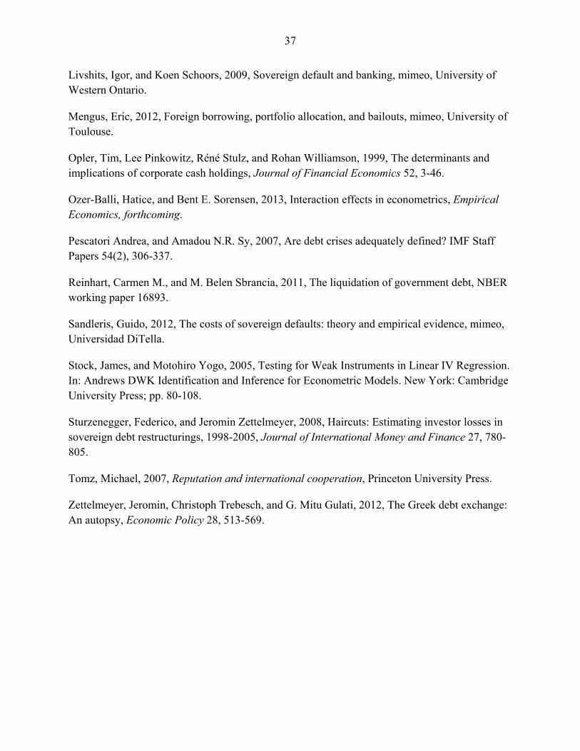
[Table I here]
Table I compares the BANKSCOPE data on bondholdings with the IMF measure. Panel
A contains the mean, the median, and the standard deviation of bondholdings (as a share of total
assets) in the full BANKSCOPE sample. Mean bondholdings are at 9.3% of assets, while median
bondholdings are approximately half as high. The standard deviation of bondholdings in the
sample is also high.12 Panel B reports somewhat lower figures for the constant-continuing
sample, where we observe also the covariates and that we use in our regression analysis. Panel C
reports the same information, but only for the subset of countries for which the IMF also reports
banks’ bondholdings. Panel D reports the IMF measure of “financial institutions’ net claims to
10 More details are found at www.prsgroup.com. 11 See, for instance, Classens and Laeven (2004), and Kalemli-Ozcan, Sorensen, and Yesiltas (2012). 12 The highest bondholdings in the sample are above 65% for selected banks in Argentina, Japan, and Venezuela in 2003; the lowest bondholdings are 0% (e.g., several U.S. banks).
14
the government,” computed as a share of total assets.13 Mean, median and standard deviation of
the IMF measure are close to the BANKSCOPE data. The IMF data gives a slightly higher mean
bondholdings, but measurement in the two datasets converges towards the end of the sample,
particularly when examining the subsample of banks in countries covered by IMF. Any
discrepancy between IMF and BANKSCOPE data is likely due to the fact that the former also
captures non-bond finance and to the fact that the banks used to compute the IMF measure may
differ from those in BANKSCOPE.
The IMF data cannot address the quality of the BANKSCOPE data on a bank-by-bank
basis. We thus compare our measure of bondholdings to the one reported by the European stress
test of 2010. This also allows us to evaluate the mismeasurement that may arise because,
differently from the stress test, BANKSCOPE does not break down bonds by nationality.
Table II reports bondholdings from the European stress tests of 2010 and 2011. Panel A
of the table reports bondholdings for the full sample contained in the stress test, whereas Panel B
reports bondholdings for the subset of the banks in the stress test sample that is contained in
BANKSCOPE. The bondholdings reported by BANKSCOPE are shown in Panel C. The data
from both sources are highly comparable. The bank-by-bank correlation between the
bondholdings reported by BANKSCOPE and by the stress test is 80%. The small discrepancies
between our measure and the stress test measure are thus most likely due to differences in the
time at which the measurement itself took place.14
13 This variable reports the net positions of commercial banks, defined as holdings of securities plus direct lending minus government deposits, and it can be interpreted as a proxy for the bondholdings of banks. Other papers using this measure are Gennaioli et al. (2014) and Kumhof and Tanner (2008). 14 While BANKSCOPE also counts non-EU bonds, the bondholdings of European banks consist primarily of EU bonds – the very reason of the stress test in the first place.
15
[Table II here]
The evidence is reassuring. Even in highly integrated European markets, where domestic
and foreign bonds are in many cases treated symmetrically by the regulatory framework, more
than 75% of bank bondholdings correspond to domestic bonds. This share is in all likelihood
much larger in the subset of developing countries that provide most of our observations on
sovereign defaults. In sum, the BANKSCOPE measure is a good proxy for the domestic public
bonds held by banks around the world, and we use it as such in the rest of the paper.
Table III reports descriptive statistics on these bondholdings around the world. Panel A
shows that in the full sample, in non-defaulting countries banks hold on average 9% of their
assets in public bonds. Among countries that default at least once in our sample, this average is
13.5% in non-default years, and increases to 14.5% of bank assets during default years. Panel A
further shows that bondholdings are much larger in financially less developed countries, as the
average bondholdings is 8.4% of assets in OECD countries and 12.4% in non-OECD countries.
Panel B reports similar, albeit somewhat smaller figures in the constant-continuing sample that
we use in our regression analysis.
[Insert Table III Here]
To conclude, consider our data on the realized returns of public bonds. Table AIII in the
Appendix contains descriptive statistics on these returns. The average annual return of public
bonds is 9.81%, with a large standard deviation of 21.37%. Countries that experience at least one
default episode in the sample have average annual returns of 14.46%, as compared with 9.70%
for countries that do not experience any defaults. OECD countries have average annual returns of
7.62%, much lower than the non-OECD annual returns of 11.61%.
16
Bond returns vary substantially over time. To show this, Figure 1 plots sovereign bond
prices for six countries that experienced at least one default over 1998-2012. The Figure depicts
a window centered on the day of the default, and bond prices are standardized to begin at 100.
[Insert Figure 1 Here]
Across these six countries, bond prices exhibit the characteristic V-shaped pattern: in particular,
prices deteriorate steadily in the year prior to the default, they reach a minimum in the months
immediately after the default, and they pick up thereafter.
Finally, we comment briefly on our two-stage process for the construction of a series of
expected returns. Table AIV in the Appendix shows the results of the first-stage estimation of
Equation (1), in which we regress bond returns on country risk-ratings. As the first three columns
of the table shows, there is a strong negative correlation between the risk ratings at time t and
realized returns at time 1.15 Taking into account that these ratings are decreasing in risk, this
result is exactly what one would expect from theory: the positive coefficients are consistent with
the notion that high bond returns compensate investors for economic, financial, and political risk.
In the second stage, we define expected returns as the fitted values of this first-stage regression.16
This is the series that we use in our regressions.
15 All three risk scores are suitable instruments for expected returns, as the F-test in the univariate regressions are close to 10 or above, mitigating concerns that the instruments are weak (see Stock and Yogo (2005)). By comparison, column (4) in Table AIV presents the result of regressing government bond returns at t on returns at t-1. While there is also a negative and significant univariate correlation, the F-test is around 3, indicating that past government bond returns is likely to be a weak instrument. As a result, we do not use it in our analysis. 16 Specifically, we use as instruments the economic score and the political score, and we include time dummies to capture variations in the global riskless interest rate. Column 5 of Table AIV presents the results for the specification that we use in the empirical analysis as the first-stage estimation of the expected returns used in Table V, columns 3 and 5. Our results in Table V are not sensitive to the choice of instruments within the three risk scores of the ICRG.
17
2.2 Summary Statistics of other Bank-Level Variables
We consider the distribution of bank characteristics in BANKSCOPE, focusing on: (i) bank size
as measured by total assets, (ii) non-cash assets, measured as the investment in assets other than
cash and other liquid securities, (iii) leverage as measured by one minus shareholders’ equity as a
share of assets, (iv) loans outstanding as a share of assets, (v) profitability as measured by
operating income over assets, (vi) exposure to the Central Bank as measured by deposits in the
Central Bank over assets, (vii) balances in the interbank market, and (viii) government
ownership, a dummy that equals one if the government owns more than 50% of the bank’s
equity. To neutralize the impact of outliers, all variables are winsorized at the 1st and 99th
percentile. Table IV provides descriptive statistics for these variables in our sample.
[Table IV here]
Panel A shows that there is a fairly large variation in bank characteristics within the
BANKSCOPE sample. The average bank invests roughly 96% of its resources in non-cash assets
(60% of which are loans, and the rest includes government bonds, debentures and other
securities), obtains 91% of its financing in the form of debt, which includes deposits (for an
average leverage ratio assets/equity of about 10), and holds 3% of its assets in central bank
reserves.17 Table AV in the appendix reports the correlations between different bank
characteristics in our sample. All correlations are statistically significant. Bank profitability is
positively correlated with size, exposure to the central bank and interbank balances, while it is
negatively correlated with non-cash assets, leverage, and loans outstanding.
17 Panel B of Table III shows the characteristics of banks involved in the stress test. These banks are much larger and extend more loans than the median BANKSCOPE bank. They also have lower exposure to the Central Bank and to other banks. Leverage and cash are instead of similar magnitude to those observed in BANKSCOPE.
18
3. Determinants of Banks’ Bondholdings
This section addresses our first question: what determines bank bondholdings? We have already
mentioned that average bondholdings are high in our data: they account for 9.3% of bank assets
in the entire sample. Moreover, there is also substantial variation in bondholdings over time. In
countries that experience at least one default, average bondholdings during default years
represent 14.5% of assets as opposed to 13.5% in non-default years. Figure 2 illustrates this by
depicting the average evolution of bondholdings across six defaulting countries, during a seven-
year window centered on the year of default.
[Insert Figure 2 here]
The figure shows that bondholdings follow a V-shaped pattern. Starting from their initial level,
they first decrease gradually as the default is approached. From there, bondholdings rise after
reaching a minimum on the year of the default itself.
Thus, the raw data already provides two interesting facts regarding bondholdings: banks
hold substantial amounts of public bonds in non-default years and they hold even more bonds
during sovereign defaults. To delve deeper into these facts and see how they relate to bank- and
country-characteristics, we turn to regression analysis.
3.1. Methodology
Let , , denote the ratio of government bonds over assets held at time by bank located in
country . We think of , , as being chosen by banks in period – 1, so that bondholdings at
19
time t are a function of the bank’s balance sheet and of the state of the economy at time – 1.18
We then run the following regression:
, , ∙ , , ∙ , ∙ , ∙ , ∙ , ,
∙ , ∙ , , , , 2
where , is a dummy variable taking value 1 if country is in default at – 1 and value 0
otherwise, , , is a vector of bank characteristics, and , is a vector of country
characteristics. We run this regression in specifications that include country dummies, time
dummies, and also their interaction. Standard errors are clustered at the bank level throughout.19
Coefficients and respectively capture the effect of bank- and country-factors on a
bank’s holdings of public bonds when the government is not in default (i.e., in “normal times”).
Coefficient captures the average impact of default on bondholdings, while and indicate
whether the association between default and bonds is heterogeneous across banks and countries.
Equation (2) thus allows us to test whether bondholdings behave differently in years of default
relative to all other years. For example, if 0, all banks tend to increase their bondholdings
during default events.
Vector , , includes bank characteristics that may affect the demand for bonds, such
as loans outstanding (which proxies for a bank’s investment opportunities), non-cash assets,
18 The use of lagged independent variables is preferable to the use of independent variables that are contemporaneous to bondholdings for two reasons. First, bank-level explanatory variables are determined jointly with bondholdings within each year. As a result, a contemporaneous formulation of Equation (1) would suffer from severe endogeneity problems. Second, the bank does not observe the aggregate final state of the economy at until the end of period itself. As a result, the forecast of macro variables performed by the bank or by the market at time will depend on the state of the economy as measured at time 1.
19 In a previous draft we clustered standard errors at the country level and obtained very similar results.
20
exposure to central bank, interbank balances, profitability, size, whether or not the bank is owned
by the government, and lagged bondholdings to control for persistence. Vector , includes
instead country-level factors that may affect the demand for bonds, such as a country’s financial
development (as measured by Private Credit to GDP and banking crises), GDP growth, and
inflation. One interesting variable to consider is the expected return of public bonds denoted by
, , which captures the expectation (at time – 1) of the time- return of public bonds of country
. As explained in Section 2, we proxy this variable with the fitted value of realized returns when
regressed on lagged country-specific risk factors, and we estimate the two-stage model with
GMM.
3.2. Results
Table V reports the estimates of different specifications of Equation (2). Columns (1)-(3) assess
the patterns of bondholdings without accounting for the interactive effects of default and by
using only time dummies. Column (4) includes interactive effects, column (5) includes country
dummies, and finally column (6) includes country*time dummies. The inclusion of dummies is
important because it allows us to control – among other things – for variations in the supply of
government bonds in a country.20 Table V only reports coefficients of variables that are
systematically significant.
[Table V here]
Consider first columns (1) and (2). Bondholdings decrease with outstanding loans, while
they increase with bank size and government ownership. In terms of country factors,
20 It could be, for instance, that governments in poorer and less financially developed countries have higher debt levels for reasons that have nothing to do with the demand of bonds by banks. The inclusion of country dummies and country*time dummies allows us to mitigate these and other omitted variables concerns.
21
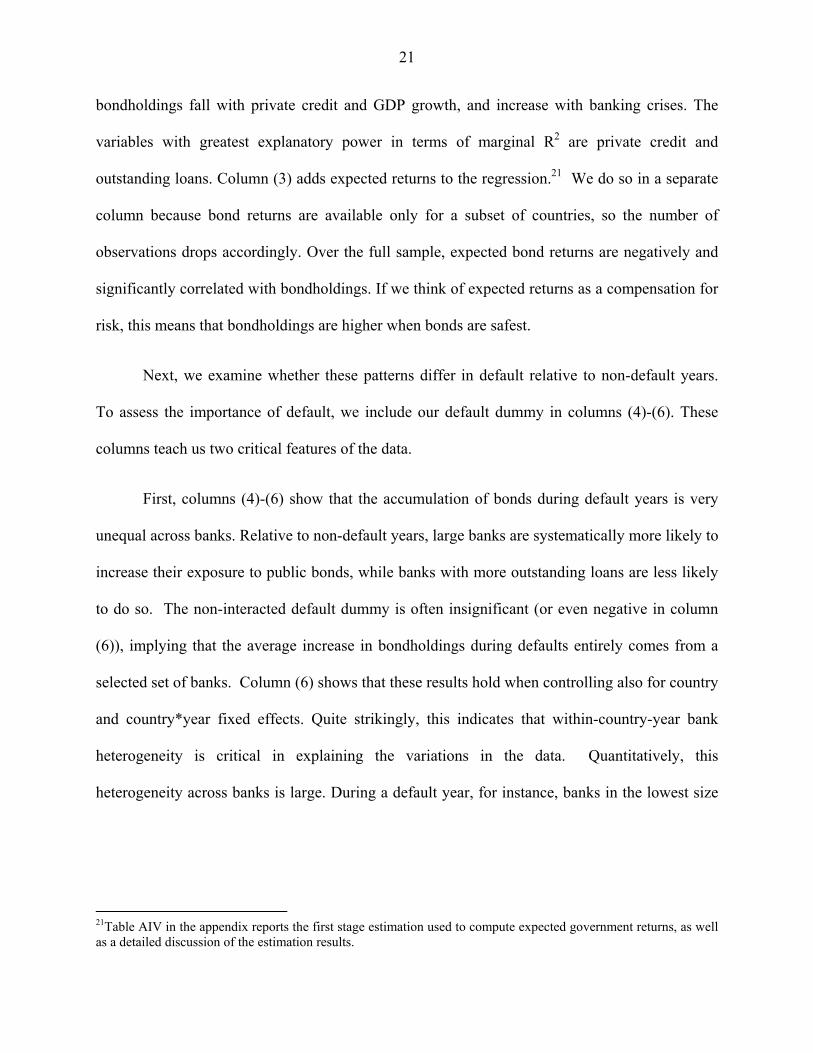
bondholdings fall with private credit and GDP growth, and increase with banking crises. The
variables with greatest explanatory power in terms of marginal R2 are private credit and
outstanding loans. Column (3) adds expected returns to the regression.21 We do so in a separate
column because bond returns are available only for a subset of countries, so the number of
observations drops accordingly. Over the full sample, expected bond returns are negatively and
significantly correlated with bondholdings. If we think of expected returns as a compensation for
risk, this means that bondholdings are higher when bonds are safest.
Next, we examine whether these patterns differ in default relative to non-default years.
To assess the importance of default, we include our default dummy in columns (4)-(6). These
columns teach us two critical features of the data.
First, columns (4)-(6) show that the accumulation of bonds during default years is very
unequal across banks. Relative to non-default years, large banks are systematically more likely to
increase their exposure to public bonds, while banks with more outstanding loans are less likely
to do so. The non-interacted default dummy is often insignificant (or even negative in column
(6)), implying that the average increase in bondholdings during defaults entirely comes from a
selected set of banks. Column (6) shows that these results hold when controlling also for country
and country*year fixed effects. Quite strikingly, this indicates that within-country-year bank
heterogeneity is critical in explaining the variations in the data. Quantitatively, this
heterogeneity across banks is large. During a default year, for instance, banks in the lowest size
21Table AIV in the appendix reports the first stage estimation used to compute expected government returns, as well as a detailed discussion of the estimation results.
22
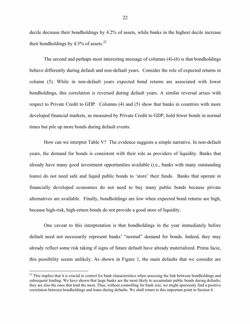
decile decrease their bondholdings by 4.2% of assets, while banks in the highest decile increase
their bondholdings by 4.5% of assets.22
The second and perhaps most interesting message of columns (4)-(6) is that bondholdings
behave differently during default and non-default years. Consider the role of expected returns in
column (5). While in non-default years expected bond returns are associated with lower
bondholdings, this correlation is reversed during default years. A similar reversal arises with
respect to Private Credit to GDP. Columns (4) and (5) show that banks in countries with more
developed financial markets, as measured by Private Credit to GDP, hold fewer bonds in normal
times but pile up more bonds during default events.
How can we interpret Table V? The evidence suggests a simple narrative. In non-default
years, the demand for bonds is consistent with their role as providers of liquidity. Banks that
already have many good investment opportunities available (i.e., banks with many outstanding
loans) do not need safe and liquid public bonds to ‘store’ their funds. Banks that operate in
financially developed economies do not need to buy many public bonds because private
alternatives are available. Finally, bondholdings are low when expected bond returns are high,
because high-risk, high-return bonds do not provide a good store of liquidity.
One caveat to this interpretation is that bondholdings in the year immediately before
default need not necessarily represent banks’ “normal” demand for bonds. Indeed, they may
already reflect some risk taking if signs of future default have already materialized. Prima facie,
this possibility seems unlikely. As shown in Figure 1, the main defaults that we consider are
22 This implies that it is crucial to control for bank characteristics when assessing the link between bondholdings and subsequent lending. We have shown that large banks are the most likely to accumulate public bonds during defaults; they are also the ones that lend the most. Thus, without controlling for bank size, we might spuriously find a positive correlation between bondholdings and loans during defaults. We shall return to this important point in Section 4.
23
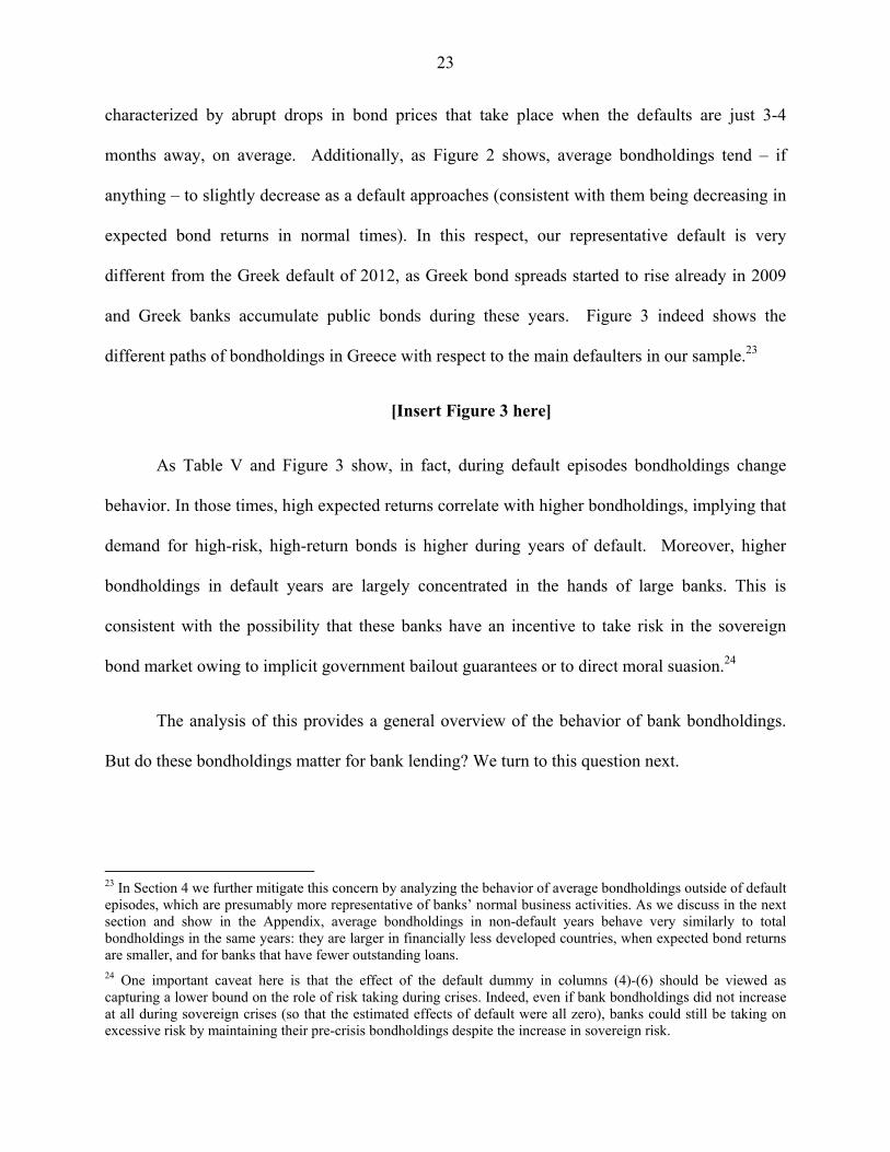
characterized by abrupt drops in bond prices that take place when the defaults are just 3-4
months away, on average. Additionally, as Figure 2 shows, average bondholdings tend – if
anything – to slightly decrease as a default approaches (consistent with them being decreasing in
expected bond returns in normal times). In this respect, our representative default is very
different from the Greek default of 2012, as Greek bond spreads started to rise already in 2009
and Greek banks accumulate public bonds during these years. Figure 3 indeed shows the
different paths of bondholdings in Greece with respect to the main defaulters in our sample.23
[Insert Figure 3 here]
As Table V and Figure 3 show, in fact, during default episodes bondholdings change
behavior. In those times, high expected returns correlate with higher bondholdings, implying that
demand for high-risk, high-return bonds is higher during years of default. Moreover, higher
bondholdings in default years are largely concentrated in the hands of large banks. This is
consistent with the possibility that these banks have an incentive to take risk in the sovereign
bond market owing to implicit government bailout guarantees or to direct moral suasion.24
The analysis of this provides a general overview of the behavior of bank bondholdings.
But do these bondholdings matter for bank lending? We turn to this question next.
23 In Section 4 we further mitigate this concern by analyzing the behavior of average bondholdings outside of default episodes, which are presumably more representative of banks’ normal business activities. As we discuss in the next section and show in the Appendix, average bondholdings in non-default years behave very similarly to total bondholdings in the same years: they are larger in financially less developed countries, when expected bond returns are smaller, and for banks that have fewer outstanding loans. 24 One important caveat here is that the effect of the default dummy in columns (4)-(6) should be viewed as capturing a lower bound on the role of risk taking during crises. Indeed, even if bank bondholdings did not increase at all during sovereign crises (so that the estimated effects of default were all zero), banks could still be taking on excessive risk by maintaining their pre-crisis bondholdings despite the increase in sovereign risk.
24
4. Default, Bondholdings and Loans
Equipped with the results of the previous section, we now address our second question: what is
the relationship between bondholdings and lending during default events?
4.1. Methodology
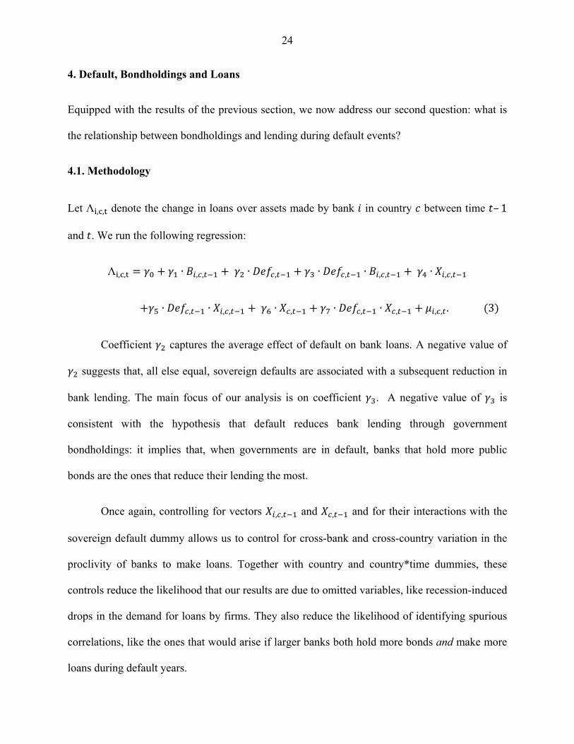
Let Λ , , denote the change in loans over assets made by bank in country between time – 1
and . We run the following regression:
Λ , , ∙ , , ∙ , ∙ , ∙ , , ∙ , ,
∙ , ∙ , , ∙ , ∙ , ∙ , , , . 3
Coefficient captures the average effect of default on bank loans. A negative value of
suggests that, all else equal, sovereign defaults are associated with a subsequent reduction in
bank lending. The main focus of our analysis is on coefficient . A negative value of is
consistent with the hypothesis that default reduces bank lending through government
bondholdings: it implies that, when governments are in default, banks that hold more public
bonds are the ones that reduce their lending the most.
Once again, controlling for vectors , , and , and for their interactions with the
sovereign default dummy allows us to control for cross-bank and cross-country variation in the
proclivity of banks to make loans. Together with country and country*time dummies, these
controls reduce the likelihood that our results are due to omitted variables, like recession-induced
drops in the demand for loans by firms. They also reduce the likelihood of identifying spurious
correlations, like the ones that would arise if larger banks both hold more bonds and make more
loans during default years.
25
The interpretation of coefficient raises an interesting question. If higher bonds are
indeed associated with a stronger drop in loans (i.e. 0) in default years, is this drop related
to the bonds that banks normally purchase in non-default years or to the bonds purchased during
the default events themselves? As we discuss in Section 5, this distinction is important: shedding
light on whether the dangerous embrace between the government and banks originates in normal
times or in the proximity of sovereign defaults has important positive and normative
implications. We address this question in three alternative ways.
First, we run a cross sectional version of Equation (3) focusing on the change in loans
around default episodes. In this regression, the dependent variable is the change in a bank’s loan-
to-asset ratio occurring in the first two years of default, while the main explanatory variable is
the bank’s bondholdings in the year prior to default. This is the simplest way to check whether
pre-default bondholdings matter. One shortcoming here is that bondholdings in the year before
default may be influenced by the anticipation of default by the bank. As a result, we perform a
second test in which the explanatory variable is a bank’s average bondholdings in the three years
prior to the default. This test allows us to establish whether or not the change in a bank’s lending
behavior around a default event is related to the public bonds that the bank has well before the
default event, before sovereign risk materializes.
While useful, this last test has still two shortcomings. First, its cross sectional nature does
not allow us to control for a full set of country*time dummies. Second, by considering only
bonds accumulated for the most part well before default, this test does not allow us to properly
assess the impact of bondholdings accumulated in the run-up to and during the default itself,
which may be an important part of the story.
26
We address these concerns by running yet another specification of Equation (2), in which
we decompose a bank’s holdings of public bonds , into: (i) a “normal-times” average
component , , measuring a bank’s average bondholdings in all non-default years up to year t,
and; (ii) a “residual” component , , , , , which captures any differential take-up in
public bonds relative to the normal-times average. We then use these components as separate
explanatory variables in Equation (2). Because this regression uses the full panel structure of our
data, it can include a full set of country*time dummies.
To interpret this regression, we view the component , , as capturing a bank’s average
demand for bonds in the course of its everyday business activity. Hence, the interaction of , ,
with the default dummy proxies for the effect of sovereign defaults that is transmitted through
the bonds that are normally held by bank i for its regular operations.25 According to this
interpretation, the residual , captures any discrepancy between observed bondholdings and
typical bondholdings in normal times. This discrepancy may be due to a number of reasons,
including – as we have mentioned – distorted incentives to accumulate bonds precisely when
they are risky.
4.2. Results
Table VI reports our estimates. Columns (1)-(4) include as explanatory variables the total
bondholdings of bank i in year – 1, , , , as well as our sovereign default dummy, various
bank-level controls, the realized return of bonds,26 and their interactions. Column (1) report
25 The effect of , , on loans during defaults could capture both the fact that default exerts an adverse balance sheet effect on banks with higher average bondholdings in normal times, and the fact that defaults reduce the appeal of bonds as liquid assets and this is costly for banks that normally use bonds for that reason. 26 We do not include other country-level controls because doing so drastically reduces the number of observations. To control for all country-level, time-varying factors, columns (4) and (5) also include country*year dummies.
27
results of a specification without any fixed effects. It shows that bondholdings have a large
negative effect on subsequent lending during default years.
[Table VI here]
Column (2) presents estimation results with year dummies but without country dummies;
column (3) presents results with year and country dummies, to control for time-invariant
country-level differences in the quality of economic policy and other institutional differences;
column (4) presents estimation results with year, country, and country*year dummies, to control
for uniform demand shocks at the country-year level. The results confirm a strong negative
effect of bondholdings on subsequent lending during default years. Column (5) repeats this test
in the full sample, i.e., including also the countries for which we do not observe sovereign bond
returns, and shows that our result is, if anything, stronger. Remarkably, columns (4) and (5) show
that within the same defaulting country-year, it is the banks most loaded with government bonds
that reduce their lending the most. This is the basic result of this section. This raises a question:
is this association driven by the bonds accumulated in non-default years or by those accumulated
during the default event itself?
Columns (6) and (7) address this question by looking at the cross-sectional variation in
changes in loans around a default and seeing how it correlates with bonds held before the default.
Column (6) shows that the bonds held in the year before the default have a strong negative
association with the subsequent decrease in lending during the first two years of a default event.
This finding suggests that the bonds accumulated prior to default matter for the decrease in
lending. However, it could still be that bank purchases of bonds in the year prior to default
reflect the deteriorating prospects of sovereign risk and not their regular business activity.
28
To address this possibility, in column (7) we focus on the average bondholdings held by
the banks in the three years prior to the beginning of default, to attempt to better capture the
effect of bondholdings held during the course of banks’ ‘normal’ business activity. Column (7)
shows a strong negative association between a bank’s average bondholdings in the three years
prior to a default and its change in loans during the first two years of a default event. The effects
are quantitatively large: a 10% increase in the average level of bondholdings in the three years
before default is associated with a 3.6% cumulative reduction in loans during the first two years
in default. This result is consistent with a standard balance sheet effect, whereby losses on pre-
existing government bonds reduce bank capital, forcing the bank to deleverage and thus reducing
its ability to intermediate funds towards investment. It is important to stress that these tests
require bank data for a five-year window around a default, so that they effectively focus on large
banks in large defaulting countries such as for example Argentina, Greece, and Ecuador. These
results suggest that the effects of bondholdings on lending are pervasive, long-lasting and not
limited to small banks that may go bust during the crisis.
Finally, columns (8) and (9) address this question in an alternative way, by splitting
bonds into their “normal-times” and “residual components” as defined in Section 4.1. Column
(8) introduces both variables while controlling for country dummies, time dummies, bank
controls, and expected returns, as well as for their interactions with default. Thus, column (8)
effectively amounts to a ‘decomposed version’ of column (3). Column (9) then adds
country*year fixed effects, so it effectively amounts to a decomposed version of columns (5).
We obtain two important results.
First, higher normal-times bonds are indeed associated with significantly fewer loans
during default events. Second, the interaction of the residual component of bonds and the default
29
dummy is also negative and significant, indicating that banks holding abnormally many bonds
during default years are systematically less likely to make new loans. This negative association is
interesting because, as we documented in Section 3, it is the large banks that are most likely to
accumulate bonds during default years. Presumably, these banks also face strong investment
opportunities. As a result, the drop in their loans during default seems likely to be induced by the
bonds that they hold, and not by a drop in their relative demand for credit.
The estimates of column (7) may be contaminated by country-level unobserved shocks,
though, such as a pre-existent decline in demand for credit by firms in the country. To rule out
this possibility, column (8) adds a full set of country*time dummies. The coefficients of both
components of bondholdings remain economically large and strongly statistically significant.
The economic effects of both the normal-time and residual component of bondholdings
are large. A 10% annual increase in the normal-time component of bondholdings within a
defaulting country is associated with a 2.1% decrease in lending; and a 10% annual increase in
the residual component of bondholdings within a defaulting country is associated with a 2.0%
decrease in lending.
The estimated marginal effects of the normal-time and the residual component of
bondholdings on loans are thus similar in magnitude. To properly assess the contribution of these
components, however, one needs to consider that in our sample banks tend to accumulate a much
larger proportion of bonds in the years prior to default relative to those accumulated in the
default years. In particular, in our sample of defaulting countries, average bank bondholdings
during non-default years (13% of assets) represent 87% of their average bondholdings during
default years (14.9% of assets). Coupled with the fact that in our sample banks loans as a share
30
of assets are four times larger than bondholdings (in particular, loans represent approximately
53% of total assets), our estimates imply that a one-dollar increase in bonds translate into a 60-
cent decrease in lending during default years; and that about 90% of this effect is due to the
normal-time component of bondholdings, i.e. to the average bondholdings held by banks before
the default took place.
Our data thus shows that, when a default takes place, there is a strong negative correlation
between a bank’s bondholdings and the loans that it extends. In our sample, though, the bulk of
the correlation is explained by the bonds accumulated in normal times. We discuss the economic
implications of these findings in Section 5.
Before concluding our statistical tests, we mention two robustness tests that address
important concerns regarding the results of this section. A first concern is that these results may
be driven by relatively “unimportant” defaults, because approximately one half of the default
episodes in our sample involve either small countries, or countries with a small banking sector,
or both. We address this concern thoroughly by redoing our estimation in various possible ways:
(i) we exclude the smaller defaulting countries in our sample, both as measured by GDP per
capita, and by the economic magnitude of the debt defaulted, and; (ii) we exclude the defaulting
countries with fewer than 5, 10, and 15 banks, respectively in our sample. As Table VII shows
in columns (1)-(10), these exercises strongly confirm our main results, which – if anything –
become both statistically and economically stronger. A second concern is that our default
dummy is too blunt a variable to capture default crises. We repeat our analysis using the haircut
measure of default constructed by Cruces and Trebesch (2013) and Zettelmeyer et al. (2012),
which capture the severity of a default. As Table VII, columns (11)-(11) show, our main results
are again confirmed and if anything the economic magnitude of the results is stronger. Finally,
31
we repeat our analysis using the augmented measure of default that, in addition to the default
identified by S&P, includes defaults identified as situations in which sovereign spreads exceed
1,000 basis points.27 As Table VII, columns (13)-(14) show, our main results are again
confirmed.
[Table VII here]
5 Interpretations and Implications of our Findings
What do we learn from our empirical analysis? While the main goal of our paper is descriptive,
the correlations that we document are consistent with a simple narrative of the sovereign default-
banking crisis nexus. As we already discussed at the end of Section 3, the demand for public
bonds behaves differently in default and non-default years. During non-default years, banks’
bondholdings are consistent with the liquidity services of public bonds (Holmstrom and Tirole
(1998)): banks demand low-risk public bonds when they have few investment opportunities,
particularly in less financially-developed countries. During sovereign crises, instead,
bondholdings patterns change. In those times, it is predominantly large banks that accumulate
high-risk public bonds, consistent with an important role of bailout guarantees or moral suasion.
The evidence analyzed in Section 4 then seems to indicate that all bondholdings,
regardless of their origin, hurt the ability or willingness of banks to extent new loans when
sovereign default materializes. On the one hand, banks holding on average more bonds in the
pre-default years significantly contract their loans during the default event. These banks may be
27 As discussed before, for this exercise we are limited by the availability of data on spreads, so we are effectively limited to examining the larger, economically more important defaults. In addition to the defaults in Argentina in 2001-2004, Russia in 1998-2000, Ukraine in 1998-2000, Greece in 2012, and Seychelles in 2010 identified also by S&P, the additional defaults we examine here are Ireland in 2011, Portugal in 2011 and 2012, Greece in 2011, and Ukraine in 2001.
32
cutting their loans for one or more of the following reasons: (i) losses on their existing public
bonds force them to deleverage, or relatedly; (ii) they deliberately choose to remain exposed to
sovereign risk, or finally because; (iii) the unavailability of safe public bonds prevents them from
efficiently managing their liquidity. Either way, this correlation suggests that banks’ regular
demand for bonds during normal times induces an adverse effect on bank lending once default
strikes. On the other hand, banks with high bondholdings during the default years also
significantly contract their loans. Regardless of whether these high bondholdings are due to
banks reaching for yield or to government intervention, this correlation suggests that the banks’
demand for bonds during sovereign defaults is also detrimental to lending. The typical
explanation for this effect is that purchases of bonds crowd out new loans on the asset side of
banks.
One important feature of our dataset is that, by covering a wide sample of default and
non-default years, it allows us to quantitatively evaluate the relative importance of these different
bondholdings in transmitting sovereign defaults. In this respect, our data provide a rather clear
result: in the countries and periods that we consider, average bondholdings in non-default years,
which reflect banks’ normal activity, play a significantly larger role than bonds accumulated in
the run-up to and during default years. First, the marginal adverse effect of bonds accumulated in
non-default years is slightly larger than the marginal adverse effect of bonds bought during
crises. Second, and most important, banks in our sample of defaulting countries hold many bonds
in normal times (13.0%), and the average increase in bondholdings during crises is rather small
by comparison (less than 2%).
These results provide a new perspective on the mechanisms whereby the sovereign
default-banking crisis nexus comes into existence and operates. Fueled by the recent European
33
sovereign crisis, much of the work on this nexus has focused on risk-taking by European banks
(e.g., see Acharya and Steffen (2013)). Although this may well be the right strategy for the
European context, our panoramic view of sovereign debt crises calls for paying close attention
also to the bonds held by banks in normal times: average bondholdings of banks during non-
default years appear to play a very important role in sovereign crises, and neglecting them might
be problematic. This insight has both positive and, potentially, normative implications.
From a positive standpoint, our analysis suggests that the unfolding of sovereign crises is
qualitatively different in emerging and advanced economies. In emerging economies, financial
markets are less developed and banks hold a large amount of bonds in normal times (12.7% of
assets in non-OECD countries). It is only natural that these bondholdings generate a large
fraction of the adverse effects of sovereign defaults on bank lending. In developed economies,
banks hold substantially fewer bonds in normal times (5% of assets in OECD countries). As a
result, in these countries, banks’ take-up of public bonds during crises is likely to be more
important relative to their total bondholdings. The patterns of bondholdings in our sample
confirm this hypothesis. In the defaults by emerging countries in our sample, such as for example
Argentina and Russia, banks hold many bonds before the default; if anything, they slightly
decrease their bondholding as default approaches and, after default happens, large banks
accumulate even more bonds. By contrast, banks in Europe’s more troubled economies held few
bonds before 2008, but they accumulated large quantities of them as sovereign risk increased. In
our sample, bondholdings between 2008 and 2010 went from 4.4% to 12.3% in Greek banks;
from 6.7% to 11% in Irish banks; and from 3% to 8.1% in Portuguese banks.28 It thus seems
highly likely that, in more advanced economies, the accumulation of bonds during crises (either
28 Over the same period, the increase in bondholdings was much smaller in Spanish (from 4.6% to 6%) and Italian (from 11.8% to 12.4%) banks.
34
due to a search for yield or to moral suasion) is responsible for a substantially larger portion of
the adverse costs of default.
Our results also carry some potentially important normative implications. In the context
of recent events, conventional wisdom holds that the European sovereign crisis became a
banking crisis due to the specifics of bank regulation. In particular, the fact that regulation
assigns a low risk weight to sovereign bonds even in times of crisis made it possible for banks to
gamble in the sovereign bond market without being penalized by the regulator. This
consideration is important, but our results suggest that the link between sovereign risk and
banking crisis might result from deeper forces. If banks demand a sizeable amount of
government bonds to carry out their normal business activities, as seems to be particularly the
case in emerging economies but also in developed ones, sovereign defaults will undermine the
functioning of the banking sector and bank lending over and above its risk taking during the
crisis itself. In this context, proposed regulations to increase the risk weight of government
bonds during sovereign crises may backfire, because they might exacerbate the pro-cyclicality of
bank balance sheets without having much of an effect on the link between sovereign risk and the
banking sector.
35
References
Acharya, Viral V., Itamar Drechsler, and Philipp Schnabl, 2013, A Pyrrhic victory? Bank bailouts and sovereign credit risk, Journal of Finance, forthcoming.
Acharya, Viral V., and Raghuram G. Rajan, 2013, Sovereign debt, government myopia, and the financial sector, Review of Financial Studies 26, 1526-1560.
Acharya, Viral V., and Sascha Steffen, 2013, The greatest carry trade ever? Understanding Eurozone bank risks, NBER working paper 19039.
Andritzky, Jochen R. 2012, Government bonds and their investors: What are the facts and do they matter?, IMF working paper.
Arellano, Cristina, 2008, Default risk and income fluctuations in emerging economies, American Economic Review 98, 690-712.
Arteta, Carlos, and Galina Hale, 2008, Sovereign debt crises and credit to the private sector, Journal of International Economics 74, 53-69.
Baskaya, Yusuf Soner, and Sebnem Kalemli-Ozcan, 2014, Government debt and financial repression: Evidence from a rare disaster, University of Maryland working paper.
Battistini, Niccolò, Marco Pagano, and Saverio Simonelli, 2013, Systemic risk, sovereign yields and bank exposures in the Euro crisis, mimeo, Università di Napoli Federico II.
Beck, Thorsten, Asli Demirgüç-Kunt, and Ross Levine, 2000, A new database on financial development and structure, World Bank Economic Review 14, 597-605.
Berger, Allen, Christa Bouwman, Thomas Kick, and Klaus Schaeck, 2012, Bank risk taking and liquidity creation following regulatory interventions and capital support, mimeo, Case Western Reserve University.
Borensztein, Eduardo, and Ugo Panizza, 2008, The costs of sovereign default, IMF working paper.
Broner, Fernando, Alberto Martin, and Jaume Ventura, 2010, Sovereign risk and secondary markets, American Economic Review 100, 1523-1555.
Broner, Fernando, and Jaume Ventura, 2011, Globalization and risk sharing, Review of Economic Studies 78, 49-82.
Brutti, Filippo, and Philip Sauré, 2013, Repatriation of Debt in the Euro Crisis: Evidence for the Secondary Market Theory, mimeo, University of Zurich.
36
Claessens, Stijn, and Luc Laeven, 2004, What drives bank competition? Some international evidence, Journal of Money, Credit and Banking 36, 563-583.
Comelli, Fabio, 2012, Emerging market sovereign bond spreads: Estimation and back-testing, IMF working paper.
Cruces, Juan J., and Christoph Trebesch, 2013, Sovereign defaults: The price of haircuts, American Economic Journal: Macroeconomics 5, 85-117.
Eaton, Jonathan, and Mark Gersovitz, 1981, Debt with potential repudiation: Theoretical and empirical analysis, Review of Economic Studies 48, 289-309.
Gelos, R. Gaston, Sahay Ratna and Guido Sandleris, 2011, Sovereign borrowing by developing countries: What determines market access?, Journal of International Economics 83(2), pages 243-254.
Gennaioli, Nicola, Alberto Martin, and Stefano Rossi, 2014, Sovereign default, domestic banks, and financial institutions, Journal of Finance 69, 819-866.
Greenwood, Robin, and Dimitri Vayanos, 2014, Bond supply and excess bond returns, Review of Financial Studies 27, 663-713.
Hannoun, Hervé, 2011, Sovereign risk in bank regulation and supervision: Where do we stand?, Bank for International Settlements.
Holmström, Bengt, and Jean Tirole, 1993, Market liquidity and performance monitoring, Journal of Political Economy 101, 678-709.
Kalemli-Ozcan, Sebnem, Bent E. Sorensen and Sevcan Yesiltas, 2012, Leverage across banks, firms and countries, Journal of International Economics 88, 284-298.
Kim, Gloria, 2010, EMBI Global and EMBI Global Diversified, rules and methodology, Global Research Index Research, J.P. Morgan Securities Inc.
Krishnamurthy, Arvind and Annette Vissing-Jorgensen, 2012, The aggregate demand for treasury debt, Journal of Political Economy 120, 233-267.
Kumhof, Michael, and Evan Tanner, 2008, Government debt: A key role in financial intermediation, in Carmen M. Reinhart, Carlos Végh, and Andres Velasco, eds.: Money, Crises and Transition, Essays in Honor of Guillermo A. Calvo.
Levy-Yeyati, Eduardo, Maria Soledad Martinez Peria, and Sergio Schmukler, 2010, Depositor behavior under macroeconomic risk: Evidence from bank runs in emerging economies, Journal of Money, Credit, and Banking 42, 585-614.
37
Livshits, Igor, and Koen Schoors, 2009, Sovereign default and banking, mimeo, University of Western Ontario.
Mengus, Eric, 2012, Foreign borrowing, portfolio allocation, and bailouts, mimeo, University of Toulouse.
Opler, Tim, Lee Pinkowitz, Réné Stulz, and Rohan Williamson, 1999, The determinants and implications of corporate cash holdings, Journal of Financial Economics 52, 3-46.
Ozer-Balli, Hatice, and Bent E. Sorensen, 2013, Interaction effects in econometrics, Empirical Economics, forthcoming.
Pescatori Andrea, and Amadou N.R. Sy, 2007, Are debt crises adequately defined? IMF Staff Papers 54(2), 306-337.
Reinhart, Carmen M., and M. Belen Sbrancia, 2011, The liquidation of government debt, NBER working paper 16893.
Sandleris, Guido, 2012, The costs of sovereign defaults: theory and empirical evidence, mimeo, Universidad DiTella.
Stock, James, and Motohiro Yogo, 2005, Testing for Weak Instruments in Linear IV Regression. In: Andrews DWK Identification and Inference for Econometric Models. New York: Cambridge University Press; pp. 80-108.
Sturzenegger, Federico, and Jeromin Zettelmeyer, 2008, Haircuts: Estimating investor losses in sovereign debt restructurings, 1998-2005, Journal of International Money and Finance 27, 780-805.
Tomz, Michael, 2007, Reputation and international cooperation, Princeton University Press.
Zettelmeyer, Jeromin, Christoph Trebesch, and G. Mitu Gulati, 2012, The Greek debt exchange: An autopsy, Economic Policy 28, 513-569.
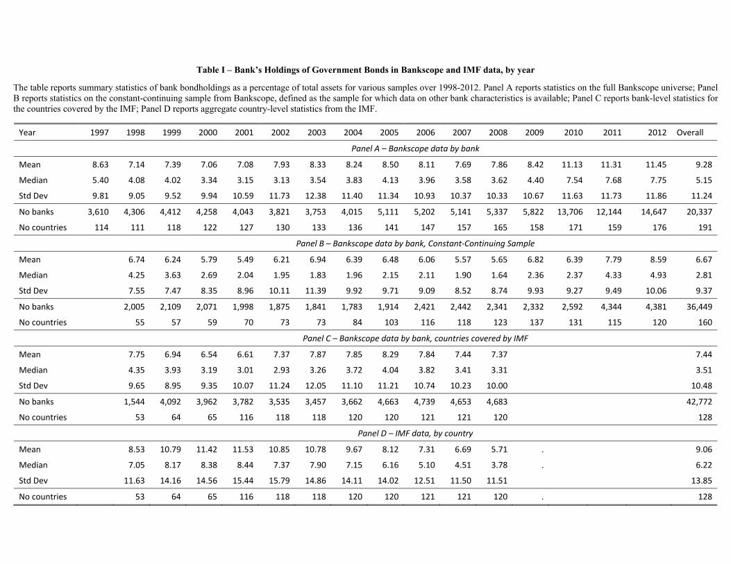
Table I – Bank’s Holdings of Government Bonds in Bankscope and IMF data, by year
The table reports summary statistics of bank bondholdings as a percentage of total assets for various samples over 1998-2012. Panel A reports statistics on the full Bankscope universe; Panel B reports statistics on the constant-continuing sample from Bankscope, defined as the sample for which data on other bank characteristics is available; Panel C reports bank-level statistics for the countries covered by the IMF; Panel D reports aggregate country-level statistics from the IMF.
Year 1997 1998 1999 2000 2001 2002 2003 2004 2005 2006 2007 2008 2009 2010 2011 2012 Overall
Panel A – Bankscope data by bank
Mean 8.63 7.14 7.39 7.06 7.08 7.93 8.33 8.24 8.50 8.11 7.69 7.86 8.42 11.13 11.31 11.45 9.28
Median 5.40 4.08 4.02 3.34 3.15 3.13 3.54 3.83 4.13 3.96 3.58 3.62 4.40 7.54 7.68 7.75 5.15
Std Dev 9.81 9.05 9.52 9.94 10.59 11.73 12.38 11.40 11.34 10.93 10.37 10.33 10.67 11.63 11.73 11.86 11.24
No banks 3,610 4,306 4,412 4,258 4,043 3,821 3,753 4,015 5,111 5,202 5,141 5,337 5,822 13,706 12,144 14,647 20,337
No countries 114 111 118 122 127 130 133 136 141 147 157 165 158 171 159 176 191
Panel B – Bankscope data by bank, Constant-Continuing Sample
Mean 6.74 6.24 5.79 5.49 6.21 6.94 6.39 6.48 6.06 5.57 5.65 6.82 6.39 7.79 8.59 6.67
Median 4.25 3.63 2.69 2.04 1.95 1.83 1.96 2.15 2.11 1.90 1.64 2.36 2.37 4.33 4.93 2.81
Std Dev 7.55 7.47 8.35 8.96 10.11 11.39 9.92 9.71 9.09 8.52 8.74 9.93 9.27 9.49 10.06 9.37
No banks 2,005 2,109 2,071 1,998 1,875 1,841 1,783 1,914 2,421 2,442 2,341 2,332 2,592 4,344 4,381 36,449
No countries 55 57 59 70 73 73 84 103 116 118 123 137 131 115 120 160
Panel C – Bankscope data by bank, countries covered by IMF
Mean 7.75 6.94 6.54 6.61 7.37 7.87 7.85 8.29 7.84 7.44 7.37 7.44
Median 4.35 3.93 3.19 3.01 2.93 3.26 3.72 4.04 3.82 3.41 3.31 3.51
Std Dev 9.65 8.95 9.35 10.07 11.24 12.05 11.10 11.21 10.74 10.23 10.00 10.48
No banks 1,544 4,092 3,962 3,782 3,535 3,457 3,662 4,663 4,739 4,653 4,683 42,772
No countries 53 64 65 116 118 118 120 120 121 121 120 128
Panel D – IMF data, by country
Mean 8.53 10.79 11.42 11.53 10.85 10.78 9.67 8.12 7.31 6.69 5.71 . 9.06
Median 7.05 8.17 8.38 8.44 7.37 7.90 7.15 6.16 5.10 4.51 3.78 . 6.22
Std Dev 11.63 14.16 14.56 15.44 15.79 14.86 14.11 14.02 12.51 11.50 11.51 13.85
No countries 53 64 65 116 118 118 120 120 121 121 120 . 128
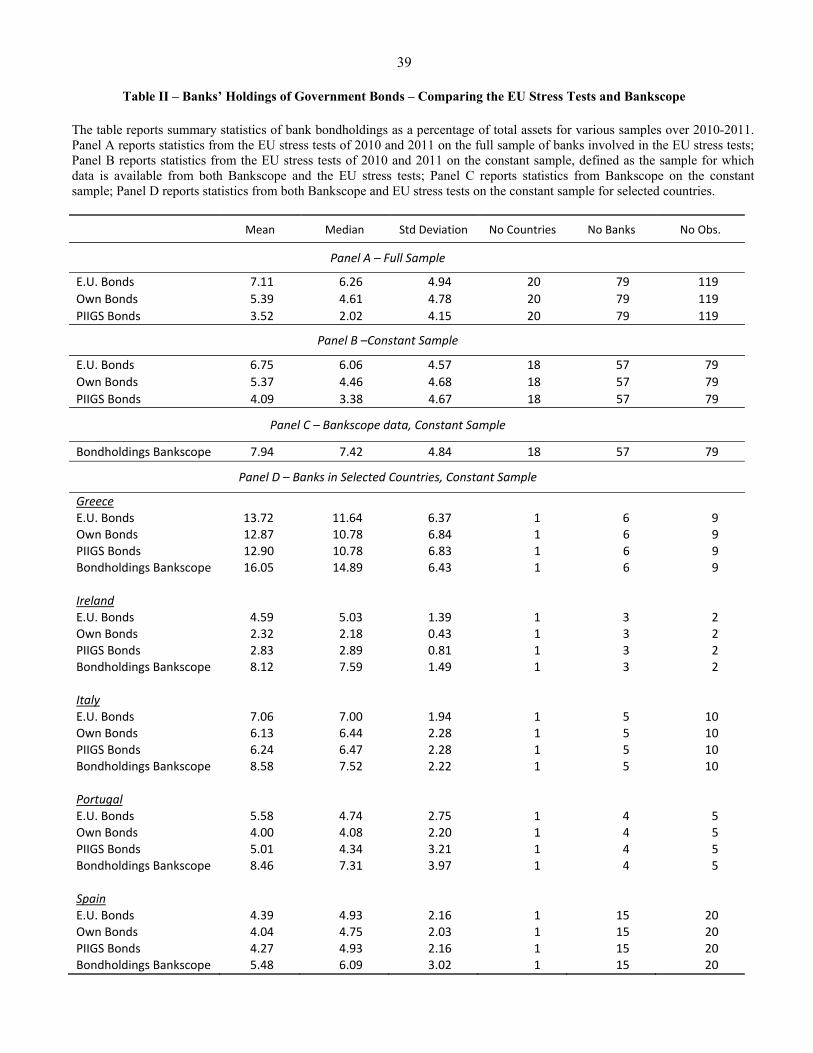
39
Table II – Banks’ Holdings of Government Bonds – Comparing the EU Stress Tests and Bankscope
The table reports summary statistics of bank bondholdings as a percentage of total assets for various samples over 2010-2011. Panel A reports statistics from the EU stress tests of 2010 and 2011 on the full sample of banks involved in the EU stress tests; Panel B reports statistics from the EU stress tests of 2010 and 2011 on the constant sample, defined as the sample for which data is available from both Bankscope and the EU stress tests; Panel C reports statistics from Bankscope on the constant sample; Panel D reports statistics from both Bankscope and EU stress tests on the constant sample for selected countries.
Mean Median Std Deviation No Countries No Banks No Obs.
Panel A – Full Sample
E.U. Bonds 7.11 6.26 4.94 20 79 119
Own Bonds 5.39 4.61 4.78 20 79 119
PIIGS Bonds 3.52 2.02 4.15 20 79 119
Panel B –Constant Sample
E.U. Bonds 6.75 6.06 4.57 18 57 79
Own Bonds 5.37 4.46 4.68 18 57 79
PIIGS Bonds 4.09 3.38 4.67 18 57 79
Panel C – Bankscope data, Constant Sample
Bondholdings Bankscope 7.94 7.42 4.84 18 57 79
Panel D – Banks in Selected Countries, Constant Sample
Greece E.U. Bonds 13.72 11.64 6.37 1 6 9 Own Bonds 12.87 10.78 6.84 1 6 9 PIIGS Bonds 12.90 10.78 6.83 1 6 9 Bondholdings Bankscope 16.05 14.89 6.43 1 6 9
Ireland E.U. Bonds 4.59 5.03 1.39 1 3 2 Own Bonds 2.32 2.18 0.43 1 3 2 PIIGS Bonds 2.83 2.89 0.81 1 3 2 Bondholdings Bankscope 8.12 7.59 1.49 1 3 2
Italy E.U. Bonds 7.06 7.00 1.94 1 5 10 Own Bonds 6.13 6.44 2.28 1 5 10 PIIGS Bonds 6.24 6.47 2.28 1 5 10 Bondholdings Bankscope 8.58 7.52 2.22 1 5 10
Portugal E.U. Bonds 5.58 4.74 2.75 1 4 5 Own Bonds 4.00 4.08 2.20 1 4 5 PIIGS Bonds 5.01 4.34 3.21 1 4 5 Bondholdings Bankscope 8.46 7.31 3.97 1 4 5
Spain E.U. Bonds 4.39 4.93 2.16 1 15 20 Own Bonds 4.04 4.75 2.03 1 15 20 PIIGS Bonds 4.27 4.93 2.16 1 15 20 Bondholdings Bankscope 5.48 6.09 3.02 1 15 20
40
Table III – Banks’ Holdings of Government Bonds Around the World
The table reports summary statistics of the banks’ holdings of government bonds, computed as a percentage of total assets. Panel A reports statistics on the Bankscope universe and Panel B on the constant-continuing sample.
Panel A – Bondholdings – Bankscope population Overall Non-Defaulting Defaulting Countries OECD Non-OECD
Countries Non-Default Yrs Default Yrs
Mean 9.28 9.06 13.49 14.49 8.43 12.39
Median 5.15 5.02 8.94 9.15 4.47 8.11
Std Deviation 11.24 11.03 13.90 15.35 10.60 12.85
No Banks 20,337 19,714 542 501 16,401 3,976
No Countries 191 157 34 24 34 157
No Bank-Year Ob 99,328 94,744 3,161 1,225 78,118 21,210
Panel B – Bondholdings – Constant-Continuing Sample Overall Non-Defaulting Defaulting Countries OECD Non-OECD
Countries Non-Default Yrs Default Yrs
Mean 6.67 6.19 12.96 14.87 4.61 12.63
Median 2.81 2.57 8.89 11.17 1.92 8.79
Std Deviation 9.37 8.84 12.94 13.87 7.13 12.12
No Banks 7,391 6,935 414 264 5,334 2,058
No Countries 160 144 26 17 32 128
No Bank-Year Obs. 36,449 34,030 1,784 635 27,074 9,375
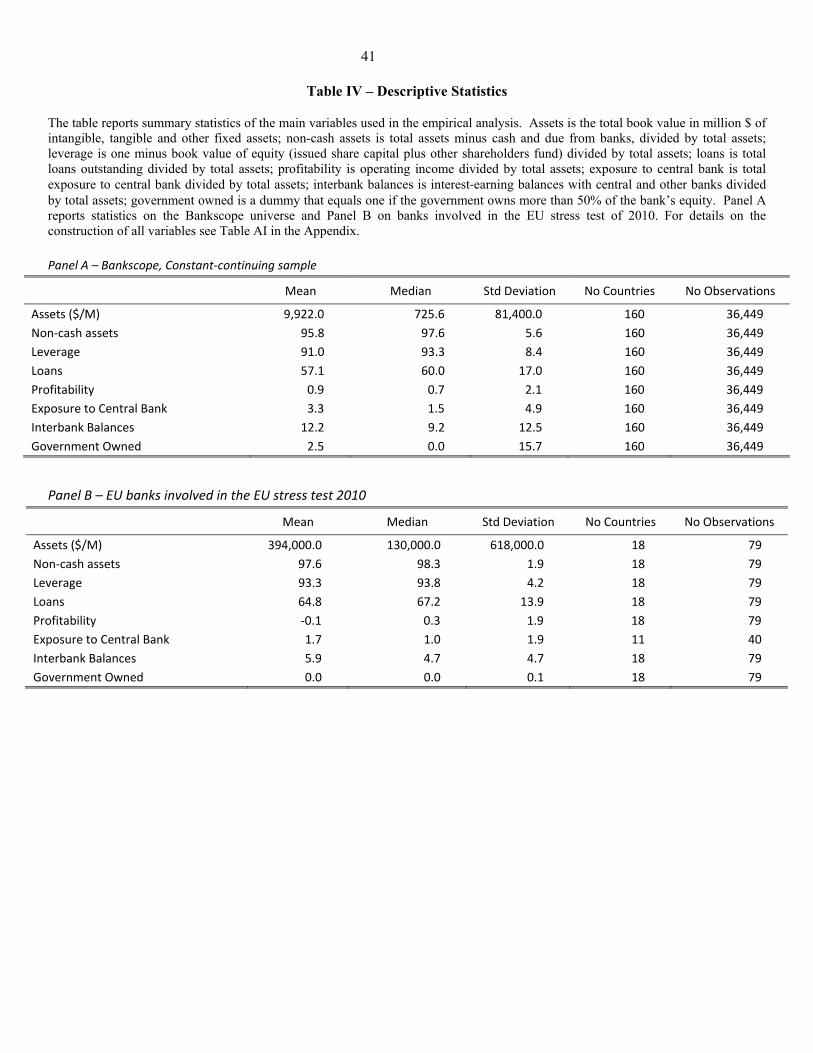
41
Table IV – Descriptive Statistics
The table reports summary statistics of the main variables used in the empirical analysis. Assets is the total book value in million $ of intangible, tangible and other fixed assets; non-cash assets is total assets minus cash and due from banks, divided by total assets; leverage is one minus book value of equity (issued share capital plus other shareholders fund) divided by total assets; loans is total loans outstanding divided by total assets; profitability is operating income divided by total assets; exposure to central bank is total exposure to central bank divided by total assets; interbank balances is interest-earning balances with central and other banks divided by total assets; government owned is a dummy that equals one if the government owns more than 50% of the bank’s equity. Panel A reports statistics on the Bankscope universe and Panel B on banks involved in the EU stress test of 2010. For details on the construction of all variables see Table AI in the Appendix.
Panel A – Bankscope, Constant-continuing sample
Mean Median Std Deviation No Countries No Observations
Assets ($/M) 9,922.0 725.6 81,400.0 160 36,449
Non-cash assets 95.8 97.6 5.6 160 36,449
Leverage 91.0 93.3 8.4 160 36,449
Loans 57.1 60.0 17.0 160 36,449
Profitability 0.9 0.7 2.1 160 36,449
Exposure to Central Bank 3.3 1.5 4.9 160 36,449
Interbank Balances 12.2 9.2 12.5 160 36,449
Government Owned 2.5 0.0 15.7 160 36,449
Panel B – EU banks involved in the EU stress test 2010
Mean Median Std Deviation No Countries No Observations
Assets ($/M) 394,000.0 130,000.0 618,000.0 18 79
Non-cash assets 97.6 98.3 1.9 18 79
Leverage 93.3 93.8 4.2 18 79
Loans 64.8 67.2 13.9 18 79
Profitability -0.1 0.3 1.9 18 79
Exposure to Central Bank 1.7 1.0 1.9 11 40
Interbank Balances 5.9 4.7 4.7 18 79
Government Owned 0.0 0.0 0.1 18 79
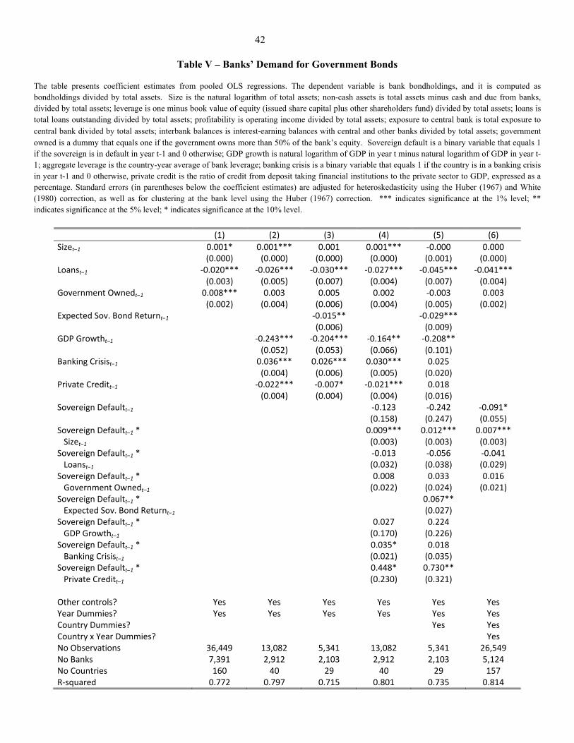
42
Table V – Banks’ Demand for Government Bonds
The table presents coefficient estimates from pooled OLS regressions. The dependent variable is bank bondholdings, and it is computed as bondholdings divided by total assets. Size is the natural logarithm of total assets; non-cash assets is total assets minus cash and due from banks, divided by total assets; leverage is one minus book value of equity (issued share capital plus other shareholders fund) divided by total assets; loans is total loans outstanding divided by total assets; profitability is operating income divided by total assets; exposure to central bank is total exposure to central bank divided by total assets; interbank balances is interest-earning balances with central and other banks divided by total assets; government owned is a dummy that equals one if the government owns more than 50% of the bank’s equity. Sovereign default is a binary variable that equals 1 if the sovereign is in default in year t-1 and 0 otherwise; GDP growth is natural logarithm of GDP in year t minus natural logarithm of GDP in year t-1; aggregate leverage is the country-year average of bank leverage; banking crisis is a binary variable that equals 1 if the country is in a banking crisis in year t-1 and 0 otherwise, private credit is the ratio of credit from deposit taking financial institutions to the private sector to GDP, expressed as a percentage. Standard errors (in parentheses below the coefficient estimates) are adjusted for heteroskedasticity using the Huber (1967) and White (1980) correction, as well as for clustering at the bank level using the Huber (1967) correction. *** indicates significance at the 1% level; ** indicates significance at the 5% level; * indicates significance at the 10% level.
(1) (2) (3) (4) (5) (6)
Sizet–1 0.001* 0.001*** 0.001 0.001*** -0.000 0.000 (0.000) (0.000) (0.000) (0.000) (0.001) (0.000)Loanst–1 -0.020*** -0.026*** -0.030*** -0.027*** -0.045*** -0.041*** (0.003) (0.005) (0.007) (0.004) (0.007) (0.004)Government Ownedt–1 0.008*** 0.003 0.005 0.002 -0.003 0.003 (0.002) (0.004) (0.006) (0.004) (0.005) (0.002)Expected Sov. Bond Returnt–1 -0.015** -0.029*** (0.006) (0.009) GDP Growtht–1 -0.243*** -0.204*** -0.164** -0.208** (0.052) (0.053) (0.066) (0.101) Banking Crisist–1 0.036*** 0.026*** 0.030*** 0.025 (0.004) (0.006) (0.005) (0.020) Private Creditt–1 -0.022*** -0.007* -0.021*** 0.018 (0.004) (0.004) (0.004) (0.016) Sovereign Defaultt–1 -0.123 -0.242 -0.091* (0.158) (0.247) (0.055)Sovereign Defaultt–1 * 0.009*** 0.012*** 0.007*** Sizet–1 (0.003) (0.003) (0.003)Sovereign Defaultt–1 * -0.013 -0.056 -0.041 Loanst–1 (0.032) (0.038) (0.029)Sovereign Defaultt–1 * 0.008 0.033 0.016 Government Ownedt–1 (0.022) (0.024) (0.021)Sovereign Defaultt–1 * 0.067** Expected Sov. Bond Returnt–1 (0.027) Sovereign Defaultt–1 * 0.027 0.224 GDP Growtht–1 (0.170) (0.226) Sovereign Defaultt–1 * 0.035* 0.018 Banking Crisist–1 (0.021) (0.035) Sovereign Defaultt–1 * 0.448* 0.730** Private Creditt–1 (0.230) (0.321) Other controls? Yes Yes Yes Yes Yes YesYear Dummies? Yes Yes Yes Yes Yes YesCountry Dummies? Yes YesCountry x Year Dummies? YesNo Observations 36,449 13,082 5,341 13,082 5,341 26,549No Banks 7,391 2,912 2,103 2,912 2,103 5,124No Countries 160 40 29 40 29 157R-squared 0.772 0.797 0.715 0.801 0.735 0.814
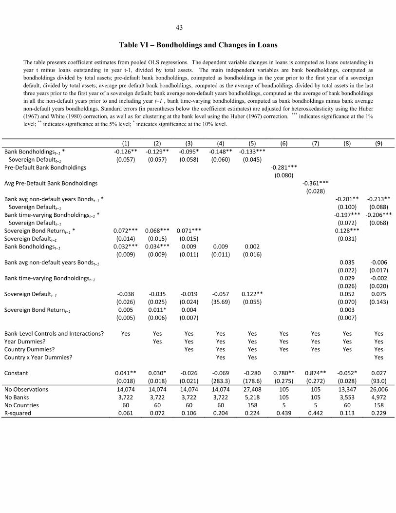
43
Table VI – Bondholdings and Changes in Loans
The table presents coefficient estimates from pooled OLS regressions. The dependent variable changes in loans is computed as loans outstanding in year t minus loans outstanding in year t-1, divided by total assets. The main independent variables are bank bondholdings, computed as bondholdings divided by total assets; pre-default bank bondholdings, coimputed as bondholdings in the year prior to the first year of a sovereign default, divided by total assets; average pre-default bank bondholdings, computed as the average of bondholdings divided by total assets in the last three years prior to the first year of a sovereign default; bank average non-default years bondholdings, computed as the average of bank bondholdings in all the non-default years prior to and including year t–1 , bank time-varying bondholdings, computed as bank bondholdings minus bank average non-default years bondholdings. Standard errors (in parentheses below the coefficient estimates) are adjusted for heteroskedasticity using the Huber (1967) and White (1980) correction, as well as for clustering at the bank level using the Huber (1967) correction. *** indicates significance at the 1% level; ** indicates significance at the 5% level; * indicates significance at the 10% level.
(1) (2) (3) (4) (5) (6) (7) (8) (9)
Bank Bondholdingst–1 * -0.126** -0.129** -0.095* -0.148** -0.133*** Sovereign Defaultt–1 (0.057) (0.057) (0.058) (0.060) (0.045) Pre-Default Bank Bondholdings -0.281*** (0.080) Avg Pre-Default Bank Bondholdings -0.361*** (0.028)Bank avg non-default years Bondst–1 * -0.201** -0.213** Sovereign Defaultt–1 (0.100) (0.088)Bank time-varying Bondholdingst–1 * -0.197*** -0.206*** Sovereign Defaultt–1 (0.072) (0.068)Sovereign Bond Returnt–1 * 0.072*** 0.068*** 0.071*** 0.128***Sovereign Defaultt–1 (0.014) (0.015) (0.015) (0.031)Bank Bondholdingst–1 0.032*** 0.034*** 0.009 0.009 0.002 (0.009) (0.009) (0.011) (0.011) (0.016) Bank avg non-default years Bondst–1 0.035 -0.006 (0.022) (0.017)Bank time-varying Bondholdingst–1 0.029 -0.002 (0.026) (0.020)Sovereign Defaultt–1 -0.038 -0.035 -0.019 -0.057 0.122** 0.052 0.075 (0.026) (0.025) (0.024) (35.69) (0.055) (0.070) (0.143)Sovereign Bond Returnt–1 0.005 0.011* 0.004 0.003 (0.005) (0.006) (0.007) (0.007) Bank-Level Controls and Interactions? Yes Yes Yes Yes Yes Yes Yes Yes YesYear Dummies? Yes Yes Yes Yes Yes Yes Yes YesCountry Dummies? Yes Yes Yes Yes Yes Yes YesCountry x Year Dummies? Yes Yes Yes Constant 0.041** 0.030* -0.026 -0.069 -0.280 0.780** 0.874** -0.052* 0.027 (0.018) (0.018) (0.021) (283.3) (178.6) (0.275) (0.272) (0.028) (93.0)
No Observations 14,074 14,074 14,074 14,074 27,408 105 105 13,347 26,006No Banks 3,722 3,722 3,722 3,722 5,218 105 105 3,553 4,972No Countries 60 60 60 60 158 5 5 60 158R-squared 0.061 0.072 0.106 0.204 0.224 0.439 0.442 0.113 0.229
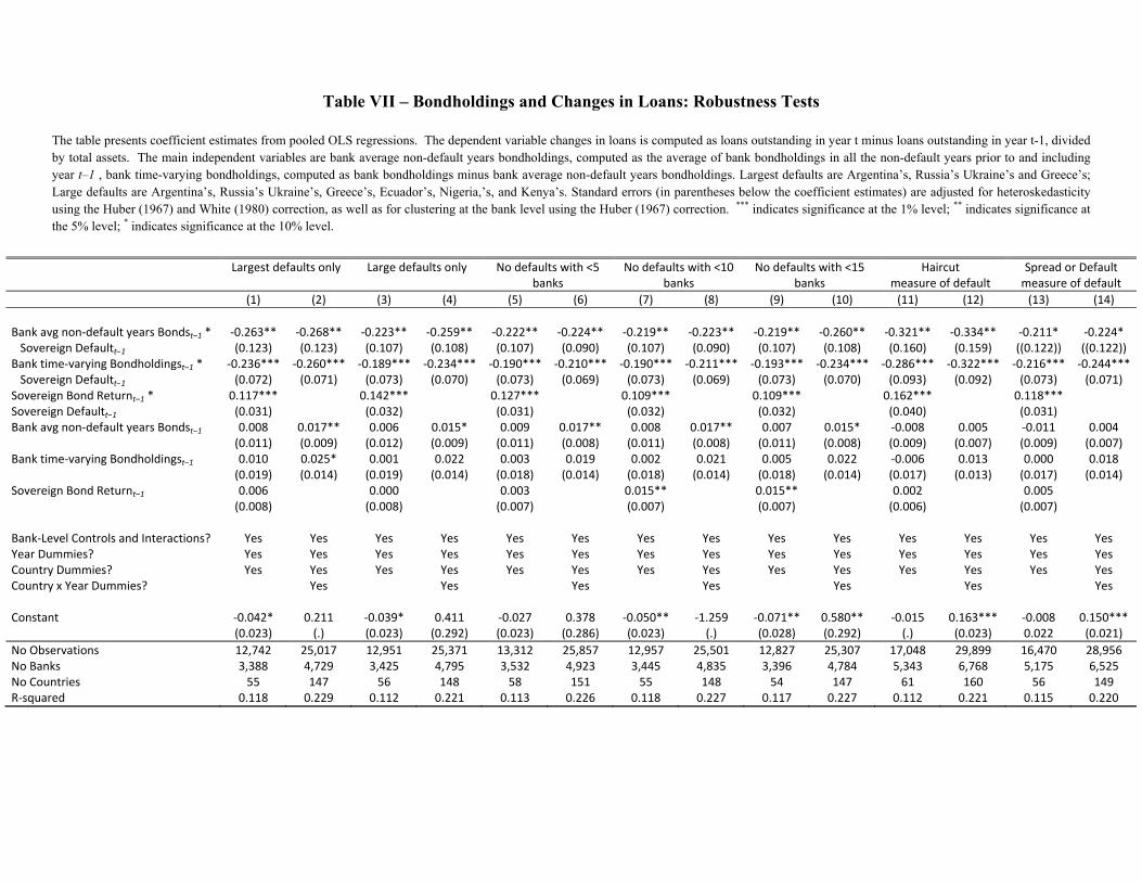
Table VII – Bondholdings and Changes in Loans: Robustness Tests
The table presents coefficient estimates from pooled OLS regressions. The dependent variable changes in loans is computed as loans outstanding in year t minus loans outstanding in year t-1, divided by total assets. The main independent variables are bank average non-default years bondholdings, computed as the average of bank bondholdings in all the non-default years prior to and including year t–1 , bank time-varying bondholdings, computed as bank bondholdings minus bank average non-default years bondholdings. Largest defaults are Argentina’s, Russia’s Ukraine’s and Greece’s; Large defaults are Argentina’s, Russia’s Ukraine’s, Greece’s, Ecuador’s, Nigeria,’s, and Kenya’s. Standard errors (in parentheses below the coefficient estimates) are adjusted for heteroskedasticity using the Huber (1967) and White (1980) correction, as well as for clustering at the bank level using the Huber (1967) correction. *** indicates significance at the 1% level; ** indicates significance at the 5% level; * indicates significance at the 10% level.
Largest defaults only Large defaults only No defaults with <5
banks No defaults with <10
banks No defaults with <15
banks Haircut
measure of default Spread or Default
measure of default
(1) (2) (3) (4) (5) (6) (7) (8) (9) (10) (11) (12) (13) (14)
Bank avg non-default years Bondst–1 * -0.263** -0.268** -0.223** -0.259** -0.222** -0.224** -0.219** -0.223** -0.219** -0.260** -0.321** -0.334** -0.211* -0.224* Sovereign Defaultt–1 (0.123) (0.123) (0.107) (0.108) (0.107) (0.090) (0.107) (0.090) (0.107) (0.108) (0.160) (0.159) ((0.122)) ((0.122)) Bank time-varying Bondholdingst–1 * -0.236*** -0.260*** -0.189*** -0.234*** -0.190*** -0.210*** -0.190*** -0.211*** -0.193*** -0.234*** -0.286*** -0.322*** -0.216*** -0.244*** Sovereign Defaultt–1 (0.072) (0.071) (0.073) (0.070) (0.073) (0.069) (0.073) (0.069) (0.073) (0.070) (0.093) (0.092) (0.073) (0.071) Sovereign Bond Returnt–1 * 0.117*** 0.142*** 0.127*** 0.109*** 0.109*** 0.162*** 0.118*** Sovereign Defaultt–1 (0.031) (0.032) (0.031) (0.032) (0.032) (0.040) (0.031) Bank avg non-default years Bondst–1 0.008 0.017** 0.006 0.015* 0.009 0.017** 0.008 0.017** 0.007 0.015* -0.008 0.005 -0.011 0.004 (0.011) (0.009) (0.012) (0.009) (0.011) (0.008) (0.011) (0.008) (0.011) (0.008) (0.009) (0.007) (0.009) (0.007) Bank time-varying Bondholdingst–1 0.010 0.025* 0.001 0.022 0.003 0.019 0.002 0.021 0.005 0.022 -0.006 0.013 0.000 0.018 (0.019) (0.014) (0.019) (0.014) (0.018) (0.014) (0.018) (0.014) (0.018) (0.014) (0.017) (0.013) (0.017) (0.014) Sovereign Bond Returnt–1 0.006 0.000 0.003 0.015** 0.015** 0.002 0.005 (0.008) (0.008) (0.007) (0.007) (0.007) (0.006) (0.007) Bank-Level Controls and Interactions? Yes Yes Yes Yes Yes Yes Yes Yes Yes Yes Yes Yes Yes Yes Year Dummies? Yes Yes Yes Yes Yes Yes Yes Yes Yes Yes Yes Yes Yes Yes Country Dummies? Yes Yes Yes Yes Yes Yes Yes Yes Yes Yes Yes Yes Yes Yes Country x Year Dummies? Yes Yes Yes Yes Yes Yes Yes Constant -0.042* 0.211 -0.039* 0.411 -0.027 0.378 -0.050** -1.259 -0.071** 0.580** -0.015 0.163*** -0.008 0.150*** (0.023) (.) (0.023) (0.292) (0.023) (0.286) (0.023) (.) (0.028) (0.292) (.) (0.023) 0.022 (0.021)
No Observations 12,742 25,017 12,951 25,371 13,312 25,857 12,957 25,501 12,827 25,307 17,048 29,899 16,470 28,956 No Banks 3,388 4,729 3,425 4,795 3,532 4,923 3,445 4,835 3,396 4,784 5,343 6,768 5,175 6,525 No Countries 55 147 56 148 58 151 55 148 54 147 61 160 56 149 R-squared 0.118 0.229 0.112 0.221 0.113 0.226 0.118 0.227 0.117 0.227 0.112 0.221 0.115 0.220
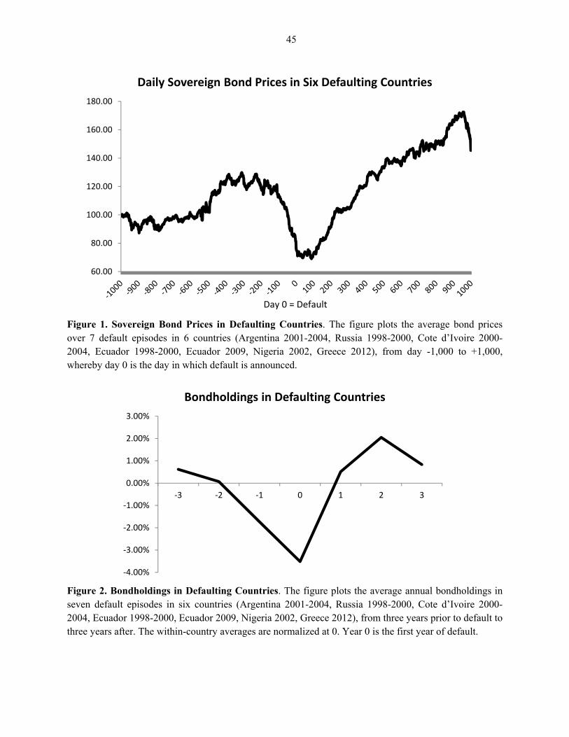
45
Figure 1. Sovereign Bond Prices in Defaulting Countries. The figure plots the average bond prices over 7 default episodes in 6 countries (Argentina 2001-2004, Russia 1998-2000, Cote d’Ivoire 2000-2004, Ecuador 1998-2000, Ecuador 2009, Nigeria 2002, Greece 2012), from day -1,000 to +1,000, whereby day 0 is the day in which default is announced.
Figure 2. Bondholdings in Defaulting Countries. The figure plots the average annual bondholdings in seven default episodes in six countries (Argentina 2001-2004, Russia 1998-2000, Cote d’Ivoire 2000-2004, Ecuador 1998-2000, Ecuador 2009, Nigeria 2002, Greece 2012), from three years prior to default to three years after. The within-country averages are normalized at 0. Year 0 is the first year of default.
60.00
80.00
100.00
120.00
140.00
160.00
180.00
Daily Sovereign Bond Prices in Six Defaulting Countries
-4.00%
-3.00%
-2.00%
-1.00%
0.00%
1.00%
2.00%
3.00%
-3 -2 -1 0 1 2 3
Bondholdings in Defaulting Countries
Day 0 = Default
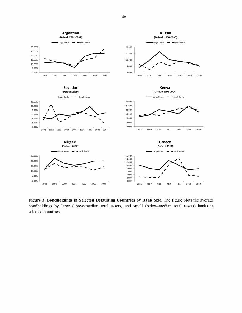
46
Figure 3. Bondholdings in Selected Defaulting Countries by Bank Size. The figure plots the average bondholdings by large (above-median total assets) and small (below-median total assets) banks in selected countries.
0.00%
5.00%
10.00%
15.00%
20.00%
25.00%
30.00%
1998 1999 2000 2001 2002 2003 2004
Argentina (Default 2001-2004)
Large Banks Small Banks
0.00%
5.00%
10.00%
15.00%
20.00%
1998 1999 2000 2001 2002 2003 2004
Russia(Default 1998-2000)
Large Banks Small Banks
0.00%
2.00%
4.00%
6.00%
8.00%
10.00%
12.00%
2001 2002 2003 2004 2005 2006 2007 2008 2009
Ecuador(Default 2009)
Large Banks Small Banks
0.00%
5.00%
10.00%
15.00%
20.00%
25.00%
30.00%
1998 1999 2000 2001 2002 2003 2004
Kenya(Default 1998-2004)
Large Banks Small Banks
0.00%
5.00%
10.00%
15.00%
20.00%
25.00%
1998 1999 2000 2001 2002 2003 2004
Nigeria(Default 2002)
Large Banks Small Banks
0.00%
2.00%
4.00%
6.00%
8.00%
10.00%
12.00%
14.00%
16.00%
2006 2007 2008 2009 2010 2011 2012
Greece(Default 2012)
Large Banks Small Banks
47
Appendix This Appendix reports tables that are referred to in the main text. Table AI lists the default events that we consider in our empirical analysis. Table AII describes our variables and their sources. Table AIII reports descriptive statistics on realized sovereign bond returns.
Table AIV presents results related to the estimation of Equation (1) in the paper, namely, the first stage of our estimation of expected sovereign bond returns, whereby realized sovereign returns are regressed on economic, financial, and political risk scores provided by the ICRG that in the literature have been found to predict sovereign returns.
The purpose of this exercise is very narrow, as we simply want to determine whether, in our sample, the country risk measures provided by the ICRG constitute valid instruments and can thus be used to construct our proxy of expected government bond returns. Our purpose is not to determine whether future government bond returns are predictable using current information publicly available to investors, which is discussed for example in Comelli (2012) and others. As a result, among other things, we are not concerned about the out-of-sample properties of our instruments.
Table AIV present the results of the first stage estimation of sovereign returns. The first three columns present the univariate correlation of annual government bond returns at year t with the economic, political, and financial risk score measured at year t-1, respectively. The correlations are large and strongly statistically significant. A higher score implies less risk, so for example, a 1-percent increase in the economic risk score translates into a 0.31% lower government return; and a 1-percent increase in the economic risk score translates into a 0.27% lower government return.
Importantly for our purposes, the F-test in these three columns is very high, around 10 or higher, which suggests that our instruments are unlikely to be weak according to the ‘rule-of-thumb’ proposed by Stock and Yogo (2005). By comparison, column (4) present the result of regressing government bond returns at t on past returns at t-1. While there is also a negative and significant univariate correlation, the F-test is around 3, indicating that past government bond returns is a likely weak instrument, and as a result we do not use it in our analysis.
Column (5) presents the specification that we use in the empirical analysis as the first stage of Table V, in Columns 3 and 5. We use as instruments the economic score and the political score, and we include time dummies to capture variations in the global riskless interest rate. It turns out that our results in Table V are not sensitive to the choice of any combination of instruments, within the three risk scores of ICRG.
The remainder of the Table shows that in-sample predictability comes from both the cross section and the time series, that is, our coefficients of interest remain strongly significant when adding time dummies and country dummies; and our main specification is also robust to the inclusion of past returns as an additional explanatory variable.
Finally, Table AV presents pair-wise correlations among the variables used in the analysis.
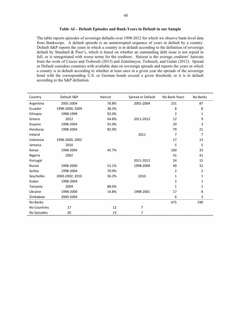
48
Table AI – Default Episodes and Bank-Years in Default in our Sample
The table reports episodes of sovereign defaults over 1998-2012 for which we observe bank-level data from Bankscope. A default episode is an uninterrupted sequence of years in default by a country. Default S&P reports the years in which a country is in default according to the definition of sovereign default by Standard & Poor’s, which is based on whether an outstanding debt issue is not repaid in full, or is renegotiated with worse terms for the creditors. Haircut is the average creditors’ haircuts from the work of Cruces and Trebesch (2013) and Zettelmeyer, Trebesch, and Gulati (2012). Spread or Default considers countries with available data on sovereign spreads and reports the years in which a country is in default according to whether at least once in a given year the spreads of the sovereign bond with the corresponding U.S. or German bonds exceed a given threshold; or it is in default according to the S&P definition.
Country Default S&P Haircut Spread or Default No Bank-Years No Banks
Argentina 2001-2004 76.8% 2001-2004 231 87
Ecuador 1998-2000; 2009 38.3% 8 8
Ethiopia 1998-1999 92.0% 2 1
Greece 2012 64.8% 2011-2012 12 9
Guyana 1998-2004 91.0% 20 3
Honduras 1998-2004 82.0% 79 21
Ireland 2011 7 7
Indonesia 1998-2000; 2002 17 13
Jamaica 2010 5 5
Kenya 1998-2004 45.7% 160 33
Nigeria 2002 41 41
Portugal 2011-2012 24 15
Russia 1998-2000 51.1% 1998-2000 40 31
Serbia 1998-2004 70.9% 2 2
Seychelles 2000-2002; 2010 56.2% 2010 1 1
Sudan 1998-2004 2 1
Tanzania 2004 88.0% 1 1
Ukraine 1998-2000 14.8% 1998-2001 17 8
Zimbabwe 2000-2004 6 3
No Banks 675 290
No Countries 17 12 7
No Episodes 20 13 7
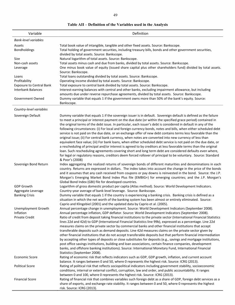
49
Table AII – Definition of the Variables used in the Analysis
Variable Definition
Bank-level variables
Assets Total book value of intangible, tangible and other fixed assets. Source: Bankscope. Bondholdings Total holding of government securities, including treasury bills, bonds and other government securities,
divided by total assets. Source: Bankscope. Size Natural logarithm of total assets. Source: Bankscope.Non-cash assets Total assets minus cash and due from banks, divided by total assets. Source: Bankscope.Leverage One minus book value of equity (issued share capital plus other shareholders fund) divided by total assets.
Source: Bankscope. Loans Total loans outstanding divided by total assets. Source: Bankscope.Profitability Operating income divided by total assets. Source: Bankscope.Exposure to Central Bank Total exposure to central bank divided by total assets. Source: Bankscope. Interbank Balances Interest-earning balances with central and other banks, excluding impairment allowance, but including
amounts due under reverse repurchase agreements, divided by total assets. Source: Bankscope. Government Owned Dummy variable that equals 1 if the government owns more than 50% of the bank’s equity. Source:
Bankscope.
Country-level variables
Sovereign Default Dummy variable that equals 1 if the sovereign issuer is in default. Sovereign default is defined as the failure to meet a principal or interest payment on the due date (or within the specified grace period) contained in the original terms of the debt issue. In particular, each issuer’s debt is considered in default in any of the following circumstances: (i) For local and foreign currency bonds, notes and bills, when either scheduled debt service is not paid on the due date, or an exchange offer of new debt contains terms less favorable than the original issue; (ii) For central bank currency, when notes are converted into new currency of less than equivalent face value; (iii) For bank loans, when either scheduled debt service is not paid on the due date, or a rescheduling of principal and/or interest is agreed to by creditors at less favorable terms than the original loan. Such rescheduling agreements covering short and long term debt are considered defaults even where, for legal or regulatory reasons, creditors deem forced rollover of principal to be voluntary. Source: Standard & Poor’s (2008)
Sovereign Bond Return Index aggregating the realized returns of sovereign bonds of different maturities and denominations in each country. Returns are expressed in dollars. The index takes into account the change in the price of the bonds and it assumes that any cash received from coupons or pay downs is reinvested in the bond. Source: the J.P. Morgan’s Emerging Market Bond Index Plus file (EMBIG+) for emerging countries; and the J.P. Morgan’s Global Bond Index (GBI) file for developed countries.
GDP Growth Logarithm of gross domestic product per capita (Atlas method). Source: World Development Indicators.Aggregate Leverage Country-year average of bank-level leverage. Source: Bankscope.Banking Crisis Dummy variable that equals 1 if the country is experiencing a banking crisis. Banking crisis is defined as a
situation in which the net worth of the banking system has been almost or entirely eliminated. Source: Caprio and Klingebiel (2001) and the updated data by Caprio et al. (2005).
Unemployment Growth Annual percentage change in unemployment. Source: World Development Indicators (September 2008).Inflation Annual percentage inflation, GDP deflator. Source: World Development Indicators (September 2008).Private Credit Ratio of credit from deposit taking financial institutions to the private sector (International Financial Statistics
lines 22d and 42d) to GDP (International Financial Statistics line 99b), expressed as a percentage. Line 22d measures claims on the private sector by commercial banks and other financial institutions that accept transferable deposits such as demand deposits. Line 42d measures claims on the private sector given by other financial institutions that do not accept transferable deposits but that perform financial intermediation by accepting other types of deposits or close substitutes for deposits (e.g., savings and mortgage institutions, post office savings institutions, building and loan associations, certain finance companies, development banks, and offshore banking institutions). Source: International Monetary Fund, International Financial Statistics (September 2008).
Economic Score Rating of economic risk that reflects indicators such as GDP, GDP growth, inflation, and current account balance. It ranges between 0 and 50, where 0 represents the highest risk. Source: ICRG (2013).
Political Score Rating of political risk that reflects sociopolitical indicators including government stability, socioeconomic conditions, internal or external conflict, corruption, law and order, and public accountability. It ranges between 0 and 100, where 0 represents the highest risk. Source: ICRG (2013).
Financial Score Rating of financial risk that combines variables such foreign debt as a share of GDP, foreign debt services as a share of exports, and exchange rate stability. It ranges between 0 and 50, where 0 represents the highest risk. Source: ICRG (2013).
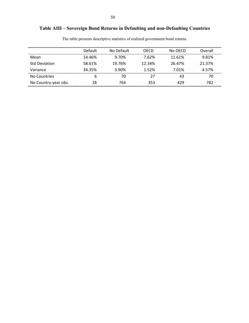
50
Table AIII – Sovereign Bond Returns in Defaulting and non-Defaulting Countries
The table presents descriptive statistics of realized government bond returns.
Default No Default OECD No OECD Overall
Mean 14.46% 9.70% 7.62% 11.61% 9.81%
Std Deviation 58.61% 19.76% 12.34% 26.47% 21.37%
Variance 34.35% 3.90% 1.52% 7.01% 4.57%
No Countries 6 70 27 43 70
No Country-year obs. 18 764 353 429 782
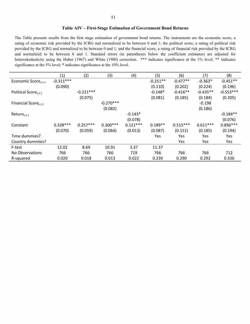
51
Table AIV – First-Stage Estimation of Government Bond Returns
The Table presents results from the first stage estimation of government bond returns. The instruments are the economic score, a rating of economic risk provided by the ICRG and normalized to be between 0 and 1; the political score, a rating of political risk provided by the ICRG and normalized to be between 0 and 1; and the financial score, a rating of financial risk provided by the ICRG and normalized to be between 0 and 1. Standard errors (in parentheses below the coefficient estimates) are adjusted for heteroskedasticity using the Huber (1967) and White (1980) correction. *** indicates significance at the 1% level; ** indicates significance at the 5% level; * indicates significance at the 10% level.
(1) (2) (3) (4) (5) (6) (7) (8)
Economic Scorec,t-1 -0.311*** -0.251** -0.477** -0.363* -0.451** (0.090) (0.110) (0.202) (0.224) (0.196) Political Scorec,t-1 -0.221*** -0.148* -0.416** -0.435** -0.553*** (0.075) (0.081) (0.185) (0.184) (0.205) Financial Scorec,t-1 -0.270*** -0.198 (0.082) (0.186) Returnc,t-1 -0.143* -0.184** (0.078) (0.076) Constant 0.328*** 0.257*** 0.300*** 0.121*** 0.189** 0.515*** 0.611*** 0.896*** (0.070) (0.059) (0.064) (0.013) (0.087) (0.151) (0.185) (0.194) Time dummies? Yes Yes Yes Yes Country dummies? Yes Yes Yes
F-test 12.02 8.69 10.91 3.37 11.37 No Observations 766 766 766 719 766 766 766 712 R-squared 0.020 0.018 0.013 0.022 0.239 0.290 0.292 0.336
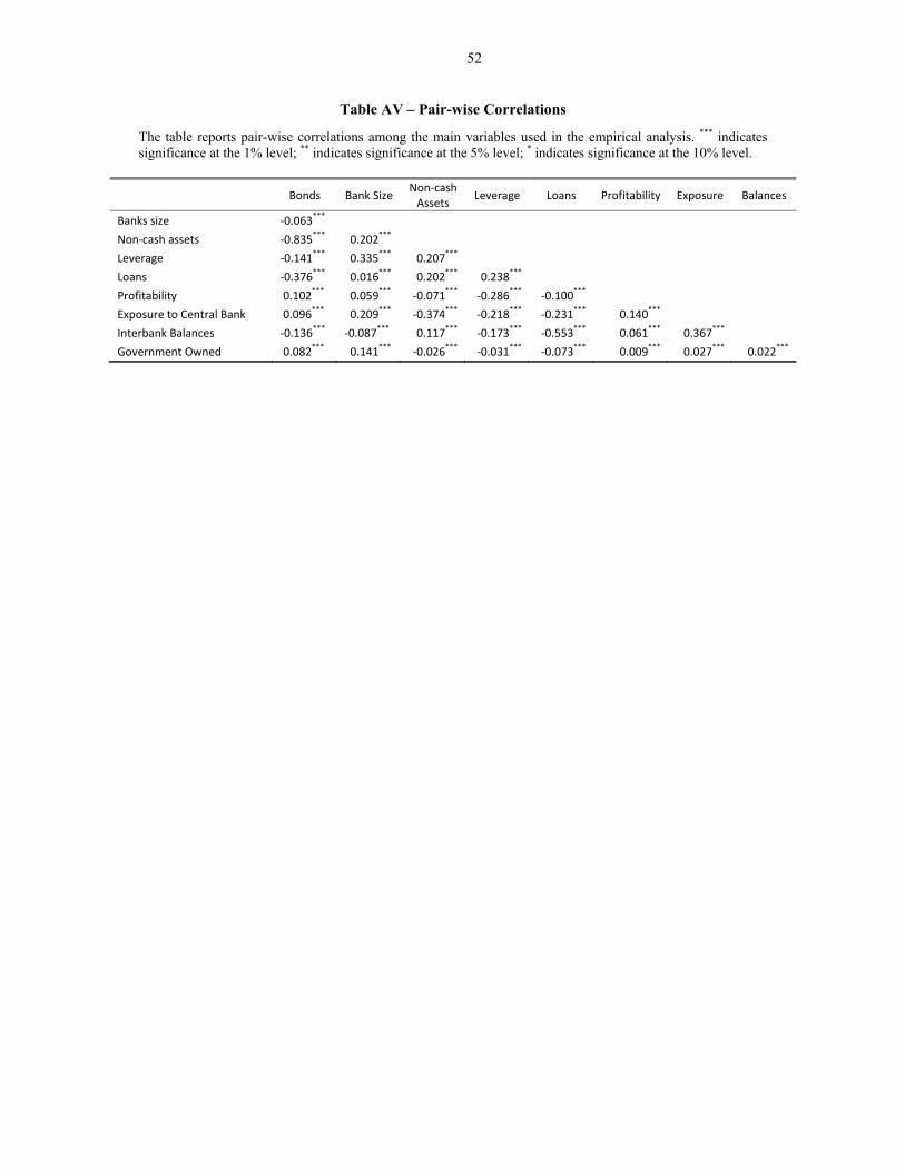
52
Table AV – Pair-wise Correlations
The table reports pair-wise correlations among the main variables used in the empirical analysis. *** indicates significance at the 1% level; ** indicates significance at the 5% level; * indicates significance at the 10% level.
Bonds Bank Size Non-cash
Assets Leverage Loans Profitability Exposure Balances
Banks size -0.063***
Non-cash assets -0.835***
0.202***
Leverage -0.141*** 0.335*** 0.207***
Loans -0.376***
0.016***
0.202***
0.238***
Profitability 0.102***
0.059***
-0.071***
-0.286***
-0.100***
Exposure to Central Bank 0.096*** 0.209*** -0.374*** -0.218*** -0.231*** 0.140***
Interbank Balances -0.136*** -0.087*** 0.117*** -0.173*** -0.553*** 0.061*** 0.367***
Government Owned 0.082***
0.141***
-0.026***
-0.031***
-0.073***
0.009***
0.027***
0.022***
Recommended