Autotuning (2/2):Specialized code generators
Prof. Richard Vuduc
Georgia Institute of Technology
CSE/CS 8803 PNA: Parallel Numerical Algorithms
[L.18] Thursday, March 6, 2008
1

Today’s sources
CS 267 at UCB (Demmel & Yelick)
Papers from various autotuning projects
PHiPAC, ATLAS, FFTW, SPIRAL, TCE
See: Proc. IEEE 2005 special issue on Program Generation, Optimization, and Platform Adaptation
Me (for once!)
2

Review:Cache-oblivious algorithms
3

A recursive algorithm for matrix-multiply
A11 A12
A21 A22
C11 C12
C21 C22
B11 B12
B21 B22Divide all dimensions in half
Bilardi, et al.: Use grey-code ordering
No. of misses, with tall-cache assumption:
Q(n) =
{8 · Q(n
2 ) if n >√
M3
3n2 otherwise
}≤ Θ
(n3
L√
M
)
4

Performance-engineering challenges
Mini-Kernel
Belady /BRILA
Scalarized /Compiler
Outer Control Structure
Iterative Recursive
Inner Control Structure
Statement Recursive
Micro-Kernel
None /Compiler
Coloring /BRILA
Iterative
ATLAS CGw/SATLAS Unleashed
5

t=0x=0 16
5
8
Cache-oblivious stencil computation
10
Theorem [Frigo & Strumpen (ICS 2005)]:d = dimension ⇒
Q(n, t; d) = O
(nd · t
M1d
)
6

Cache-conscious algorithm
Source: Datta, et al. (2007)
7

Survey of autotuning
8

Early idea seedlings
Polyalgorithms: John R. Rice
(1969) “A polyalgorithm for the automatic solution of nonlinear equations”
(1976) “The algorithm selection problem”
Profiling and feedback-directed compilation
(1971) D. Knuth: “An empirical study of FORTRAN programs”
(1982) S. Graham, P. Kessler, M. McKusick: gprof
(1991) P. Chang, S. Mahlke, W-m. W. Hwu: “Using profile information to assist classic code optimizations”
Code generation from high-level representations
(1989) J. Johnson, R.W. Johnson, D. Rodriguez, R. Tolimieri: “A methodology for designing, modifying, and implementing Fourier Transform algorithms on various architectures.”
(1992) M. Covell, C. Myers, A. Oppenheim: “Computer-aided algorithm design and arrangement” (1992)
9

Why doesn’t the compiler do the dirty work?
Why doesn’t the compiler do all of this?
Analysis
Over-specified dependencies
Correctness requirements
Limited access to relevant run-time information
Architecture: Realistic hardware models?
Engineering: Hard to modify a production compiler
10

Source: Voss, ADAPT compiler project: http://www.eecg.toronto.edu/~voss/AdaptPage/results.html
11

Source: Voss, ADAPT compiler project: http://www.eecg.toronto.edu/~voss/AdaptPage/results.html
12

Source: Voss, ADAPT compiler project: http://www.eecg.toronto.edu/~voss/AdaptPage/results.html
13
Automatic performance tuning, or“autotuning”
Two-phase methodology for producing automatically tuned code
Given: Computational kernel or program; inputs; machine
Identify and generate a parameterized space of candidate implementations
Select the fastest one using empirical modeling and automated experiments
“Autotuner” = System that implements this
Usually domain-specific (exception: “autotuning/iterative compilers”)
Leverage back-end compiler for performance and portability
14

How an autotuner differs from a compiler (roughly)
Compiler Autotuner
Input
Code generation time
Implementation selection
General-purpose source code
Specification
User responsive Long, but amortized
Static analysis; some run-time
profiling/feedback
Automated empirical models and experiments
15

m0
n0
k0 = 1 Mflop/s
Example: What a search space looks like
Source: PHiPAC Project at UC Berkeley (1997)
Platform: Sun Ultra IIi
16 double regs
667 Mflop/s peak
Unrolled, pipelined inner-kernel
Sun cc v5.0 compiler
16

17

Dense linear algebra
18

PHiPAC (1997)
Portable High-Performance ANSI C [Bilmes, Asanovic, Chin, Demmel (1997)]
Coding guidelines: C as high-level assembly language
Code generator for multi-level cache- and register-blocked matrix multiply
Exhaustive search over all parameters
Began as class project which beat the vendor BLAS
19

PHiPAC coding guideline example:Removing false dependencies
Use local variables to remove false dependencies
a[i] = b[i] + c;a[i+1] = b[i+1] * d;
float f1 = b[i];float f2 = b[i+1];
a[i] = f1 + c;a[i+1] = f2 * d;
False read-after-write hazardbetween a[i] and b[i+1]
In C99, may declare a & b unaliased(“restrict” keyword)
20

ATLAS (1998)
“Automatically Tuned Linear Algebra Software” — [R.C. Whaley and J. Dongarra (1998)]
Overcame PHiPAC shortcomings on x86 platforms
Copy optimization, prefetch, alternative schedulings
Extended to full BLAS, some LAPACK support (e.g., LU)
Code generator (written in C, output C w/ inline-assembly) with search
Copy optimization prunes much of PHiPAC’s search space
“Simple” line searches
See: iterative floating-point kernel optimizer (iFKO) work
21

Search vs. modeling
Yotov, et al. “Is search really necessary to generate high-performance BLAS?”
“Think globally, search locally”
Small gaps ⇒ local search
Large gaps ⇒ refine model
“Unleashed” ⇒ hand-optimized
plug-in kernels
22

Signal processing
23

Source: J. Johnson (2007), CScADS autotuning workshop
pseudoMflop/s
Motivation for performance tuning
24

FFTW (1997)
“Fastest Fourier Transform in the West” [M. Frigo, S. Johnson (1997)]
“Codelet” generator (in OCaml)
Explicit represent a small fixed-size transform by its computation DAG
Optimize DAG: Algebraic transformations, constant folding, “DAG transposition”
Schedule DAG cache-obliviously and output as C source code
Planner: At run-time, determine which codelets to apply
Executor: Perform FFT of a particular size using plan
Efficient “plug-in” assembly kernels
25

26

27
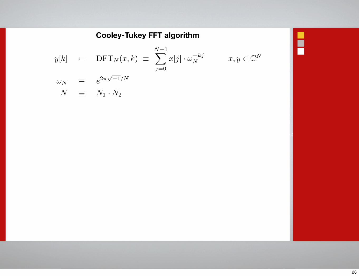
Cooley-Tukey FFT algorithm
y[k] ← DFTN (x, k) ≡N−1∑
j=0
x[j] · ω−kjN x, y ∈ CN
ωN ≡ e2π√−1/N
N ≡ N1 · N2
⇓0 ≤ k1 < N1 and 0 ≤ k2 < N2
y[k1 + k2 · N1] ←N2−1∑
n2=0
[(N1−1∑
n1
x[n1 · N2 + n2] · ω−k1n1N1
)· ω−k1n2
N
]· ω−k2n2
N2
28

Cooley-Tukey FFT algorithm
N2-point DFT
N1-point DFT Twiddle
y[k] ← DFTN (x, k) ≡N−1∑
j=0
x[j] · ω−kjN x, y ∈ CN
ωN ≡ e2π√−1/N
N ≡ N1 · N2
⇓0 ≤ k1 < N1 and 0 ≤ k2 < N2
y[k1 + k2 · N1] ←N2−1∑
n2=0
[(N1−1∑
n1
x[n1 · N2 + n2] · ω−k1n1N1
)·ω−k1n2
N
]·ω−k2n2
N2
29

Cooley-Tukey FFT algorithm: Encoding in the codelet generator
N2-point DFT
N1-point DFT Twiddle
y[k] ← DFTN (x, k) ≡N−1∑
j=0
x[j] · ω−kjN x, y ∈ CN
y[k1 + k2 · N1] ←N2−1∑
n2=0
[(N1−1∑
n1
x[n1 · N2 + n2] · ω−k1n1N1
)·ω−k1n2
N
]·ω−k2n2
N2
(Functionalpseudo-code)
let dftgen(N,x) ≡ fun k → . . . # DFTN (x, k)let cooley tukey(N1, N2, x) ≡
let x ≡ fun n2, n1 → x(n2 + n1 · N2) inlet G1 ≡ fun n2 → dftgen(N1, x(n2, )) inlet W ≡ fun k1, n2 → G1(n2, k1) · ω−k1n2
N inlet G2 ≡ fun k1 → dftgen(N2,W(k1, ))in
fun k → G2(k mod N1, k div N1)
30

Planner phase
Assembles planusing dynamicprogramming
31

32

G5
P4
33

SPIRAL (1998)
Code generator
Represent linear transformations as formulas
Symbolic algebra + rewrite engine transforms formulas
Search using variety of techniques (more later)
34

Source: J. Johnson (2007), CScADS autotuning workshop
35

Source: J. Johnson (2007), CScADS autotuning workshop
36

High-level representations and rewrite rules
DFTN ≡[ωkl
N
]0≤k,l<N
DCT-2N ≡[cos
(2l + 1)kπ
2N
]
0≤k,l<N
...
n = k · m :=⇒ DFTn → (DFTk ⊗ Im)Tn
m(Ik ⊗DFTm)Lnk
n = k · m, gcd(k, m) = 1 :=⇒ DFTn → Pn(DFTk ⊗DFTm)Qn
p is prime :=⇒ DFTp → RT
p (I1 ⊕DFTp−1Dp(I1 ⊕DFTp−1)Rp
...
DFT2 →[
1 11 −1
]
37

High-level representations expose parallelism
(I4 ⊗A) ·
X1
X2
X3
X4
=
AA
AA
·
X1
X2
X3
X4
=
AX1
AX2
AX3
AX4
A applied 4 times independently
38

High-level representations expose parallelism
SIMD-vectorizable
([a bc d
]⊗ I2
)·
x1
x2
x3
x4
=[
a · I2 b · I2
c · I2 d · I2
]·
x1
x2
x3
x4
=
a
[x1
x2
]+ b
[x3
x4
]
c
[x1
x2
]+ d
[x3
x4
]
39

Search in SPIRAL
Search over ruletrees, i.e., possible formula expansions
Empirical search
Exhaustive
Random
Dynamic programming
Evolutionary search
Hill climbing
Machine learning methods
40

Example: SMP + vectorization results
Source: F. Franchetti (2007), CScADS autotuning workshop
41

Administrivia
42

Upcoming schedule changes
Some adjustment of topics (TBD)
Tu 3/11 — Project proposals due
Th 3/13 — SIAM Parallel Processing (attendance encouraged)
Tu 4/1 — No class
Th 4/3 — Attend talk by Doug Post from DoD HPC Modernization Program
43

Homework 1:Parallel conjugate gradients
Put name on write-up!
Grading: 100 pts max
Correct implementation — 50 pts
Evaluation — 30 pts
Tested on two samples matrices — 5
Implemented and tested on stencil — 10
“Explained” performance (e.g., per proc, load balance, comp. vs. comm) — 15
Performance model — 15 pts
Write-up “quality” — 5 pts
44

Projects
Proposals due Tu 3/11
Your goal should be to do something useful, interesting, and/or publishable!
Something you’re already working on, suitably adapted for this course
Faculty-sponsored/mentored
Collaborations encouraged
45

My criteria for “approving” your project
“Relevant to this course:” Many themes, so think (and “do”) broadly
Parallelism and architectures
Numerical algorithms
Programming models
Performance modeling/analysis
46

General styles of projects
Theoretical: Prove something hard (high risk)
Experimental:
Parallelize something
Take existing parallel program, and improve it using models & experiments
Evaluate algorithm, architecture, or programming model
47

Anything of interest to a faculty member/project outside CoC
Parallel sparse triple product (R*A*RT, used in multigrid)
Future FFT
Out-of-core or I/O-intensive data analysis and algorithms
Block iterative solvers (convergence & performance trade-offs)
Sparse LU
Data structures and algorithms (trees, graphs)
Look at mixed-precision
Discrete-event approaches to continuous systems simulation
Automated performance analysis and modeling, tuning
“Unconventional,” but related
Distributed deadlock detection for MPI
UPC language extensions (dynamic block sizes)
Exact linear algebra
Examples
48

Sparse linear algebra
49

Key distinctions in autotuning work for sparse kernels
Data structure transformations
Recall HW1
Sparse data structures require meta-data overhead
Sparse matrix-vector multiply (SpMV) is memory bound
Bandwidth limited ⇒ minimize data structure size
Run-time tuning: Need lightweight techniques
Extra flops pay off
50

Sparsity (1998) and OSKI (2005)
Berkeley projects (BeBOP group: Demmel & Yelick; Im, Vuduc, et al.)
PHiPAC ⇒ SPARSITY ⇒ OSKI
On-going: See multicore optimizations by Williams, et al., in SC 2007
Motivation: Sparse matrix-vector multiply (SpMV) ≤ 10% peak or less
Indirect, irregular memory access
Low q vs. dense case
Depends on machine and matrix, possibly unknown until run-time
51

52

53
54

55

56
56

50% extra zeros
1.5x faster(2/3 time) onPentium III
57

Library Install-Time (offline) Application Run-Time
How OSKI tunes
58

Library Install-Time (offline) Application Run-Time
Benchmarkdata
1. Build forTargetArch.
2. Benchmark
Generatedcode
variants
How OSKI tunes
59

Library Install-Time (offline) Application Run-Time
Benchmarkdata
1. Build forTargetArch.
2. Benchmark
Generatedcode
variants
Heuristicmodels
1. EvaluateModels
Workloadfrom program
monitoring HistoryMatrix
2. SelectData Struct.
& Code
To user:Matrix handlefor kernelcalls
How OSKI tunes
60

Heuristic model example:Selecting a block size
Idea: Hybrid off-line/run-time model
Offline benchmark: Measure Mflops(r, c) on dense matrix in sparse format
Run-time: Sample matrix to quickly estimate Fill(r, c)
Run-time model: Choose r, c to maximize Mflops(r,c) / Fill(r, c)
Accurate in practice (selects r x c with performance within 10% of best)
Run-time cost?
Roughly 40 SpMVs
Dominated by conversion (~80%)
61
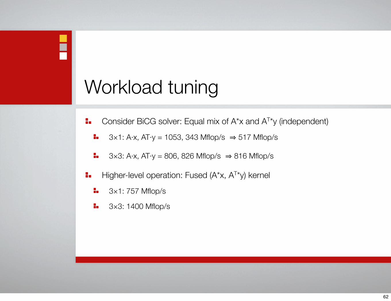
Workload tuning
Consider BiCG solver: Equal mix of A*x and AT*y (independent)
3×1: A·x, AT·y = 1053, 343 Mflop/s ⇒ 517 Mflop/s
3×3: A·x, AT·y = 806, 826 Mflop/s ⇒ 816 Mflop/s
Higher-level operation: Fused (A*x, AT*y) kernel
3×1: 757 Mflop/s
3×3: 1400 Mflop/s
62

Tensor Contraction Engine (TCE) for quantum chemistry
63

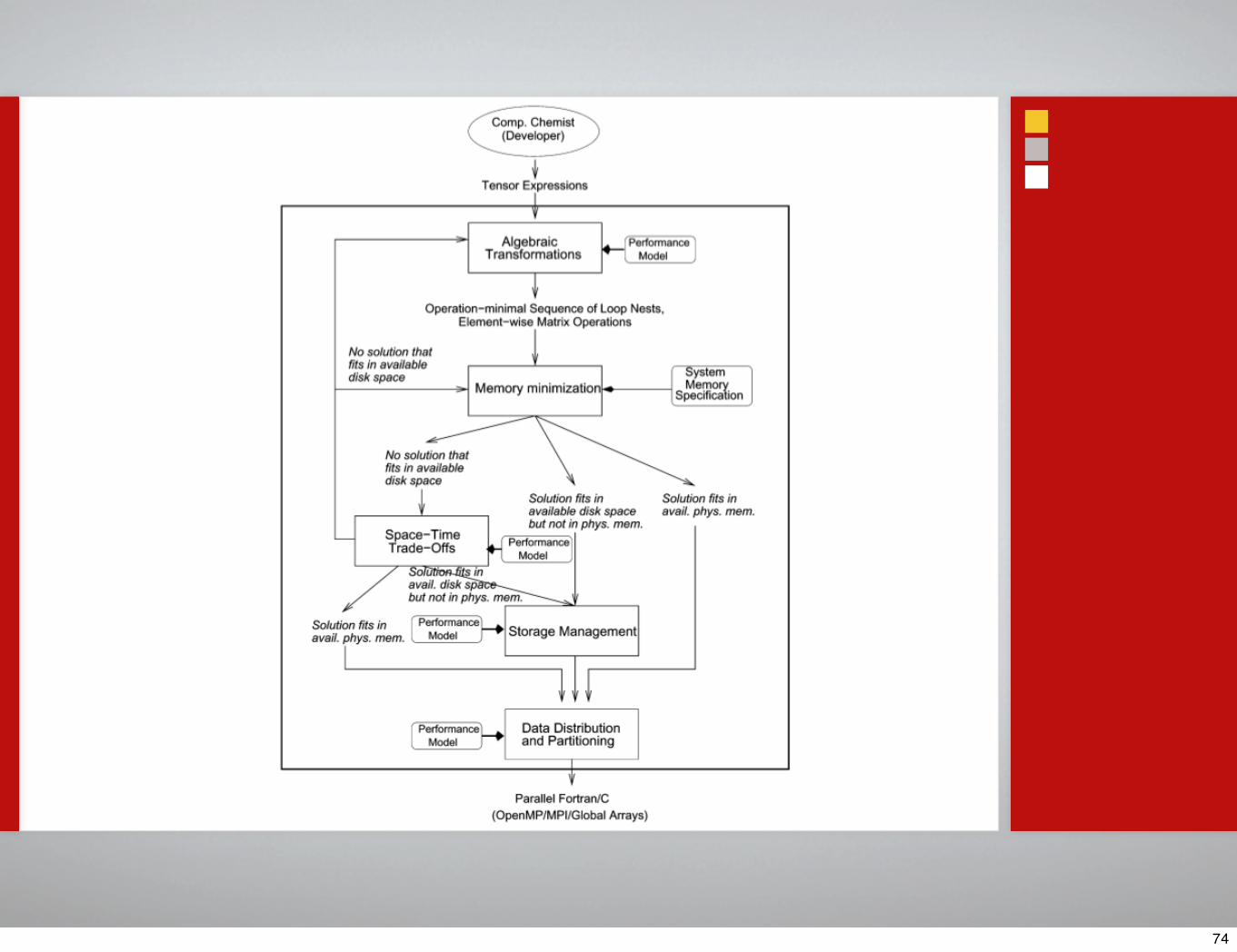
Tensor Contraction Engine (TCE)
Application domain: Quantum chemistry
Electronic structure calculations
Dominant computation expressible as a “tensor contraction”
TCE generates a complete parallel program from a high-level spec
Automates time-space trade-offs
Output
S. Hirata (2002), and many others
Following presentation taken from Proc. IEEE 2005 special issue
64

Source: Baumgartner, et al. (2005)
Motivation: Simplify program development
65

Sabij =∑
c,d,e,f,k,l
Aacik ×Bbefl × Cdfjk ×Dcdel
⇓
Sabij =∑
c,k
∑
d,f
∑
e,l
Bbefl ×Dcdel
× Cdfjk
×Aacik
Naïvely, ≈ 4 × N10 flops
Assuming associativity and distributivity, ≈ 6 × N6 flops,but also requires temporary storage.
Source: Baumgartner, et al. (2005)
Rewriting to reduce operation counts
66

T (1)bcdf =
∑
e,l
Bbefl ×Dcdel
T (2)bcjk =
∑
d,f
T (1)bcdf × Cdfjk
Sabij =∑
c,k
T (2)bcjk ×Aacik
T1 = T2 = S = 0for b, c, d, e, f, l do
T1[b, c, d, f ] += B[b, e, f, l] · D[c, d, e, l]for b, c, d, f, j, k do
T2[b, c, j, k] += T1[b, c, d, f ] · C[d, f, j, k]for a, b, c, i, j, k do
S[a, b, i, j] += T2[b, c, j, k] · A[a, c, i, k]
Operation and storage minimization via loop fusion
67

T (1)bcdf =
∑
e,l
Bbefl ×Dcdel
T (2)bcjk =
∑
d,f
T (1)bcdf × Cdfjk
Sabij =∑
c,k
T (2)bcjk ×Aacik
T1 = T2 = S = 0for b, c, d, e, f, l do
T1[b, c, d, f ] += B[b, e, f, l] · D[c, d, e, l]for b, c, d, f, j, k do
T2[b, c, j, k] += T1[b, c, d, f ] · C[d, f, j, k]for a, b, c, i, j, k do
S[a, b, i, j] += T2[b, c, j, k] · A[a, c, i, k]
Operation and storage minimization via loop fusion
S = 0for b, c do
T1f ← 0, T2f ← 0for d, f do
for e, l doT1f += B[b, e, f, l] · D[c, d, e, l]
for j, k doT2f [j, k] += T1f · C[d, f, j, k]
for a, i, j, k doS[a, b, i, j] += T2f [j, k] · A[a, c, i, k]
68

Time-space trade-offs
for a, e, c, f dofor i, j do
Xaecf += Tijae · Tijcf
for c, e, b, k do
T (1)cebk ← f1(c, e, b, k)
for a, f, b, k do
T (2)afbk ← f2(a, f, b, k)
for c, e, a, f dofor b, k do
Yceaf += T (1)cebk · T (2)
afbk
for c, e, a, f doE += Xaecf · Yceaf
Integrals, O(1000) flops
“Contraction” of T over i, j
“Contraction” over T(1) and T(2)
Max index of a—f: O(1000) i—k: O(100)
69

Time-space trade-offs
for a, e, c, f dofor i, j do
Xaecf += Tijae · Tijcf
for c, e, b, k do
T (1)cebk ← f1(c, e, b, k)
for a, f, b, k do
T (2)afbk ← f2(a, f, b, k)
for c, e, a, f dofor b, k do
Yceaf += T (1)cebk · T (2)
afbk
for c, e, a, f doE += Xaecf · Yceaf
Same indices⇒ Loop fusion candidates
Max index of a—f: O(1000) i—k: O(100)
70

Time-space trade-offs
for a, e, c, f dofor i, j do
Xaecf += Tijae · Tijcf
for c, e, b, k do
T (1)cebk ← f1(c, e, b, k)
for a, f, b, k do
T (2)afbk ← f2(a, f, b, k)
for c, e, a, f dofor b, k do
Yceaf += T (1)cebk · T (2)
afbk
for c, e, a, f doE += Xaecf · Yceaf
for a, e, c, f dofor i, j do
Xaecf += Tijae · Tijcf
for a, c, e, f , b, k do
T (1)cebk ← f1(c, e, b, k)
for a, e, c, f, b, k do
T (2)afbk ← f2(a, f, b, k)
for c, e, a, f dofor b, k do
Yceaf += T (1)cebk · T (2)
afbk
for c, e, a, f doE += Xaecf · Yceaf
Addextraflops
71

Time-space trade-offs
for a, e, c, f dofor i, j do
Xaecf += Tijae · Tijcf
for c, e, b, k do
T (1)cebk ← f1(c, e, b, k)
for a, f, b, k do
T (2)afbk ← f2(a, f, b, k)
for c, e, a, f dofor b, k do
Yceaf += T (1)cebk · T (2)
afbk
for c, e, a, f doE += Xaecf · Yceaf
⇐ Fusedfor a, e, c, f dofor i, j do
x += Tijae · Tijcf
for b, k do
T (1)cebk ← f1(c, e, b, k)
T (2)afbk ← f2(a, f, b, k)
y += T (1)cebk · T (2)
afbk
E += x · y
72
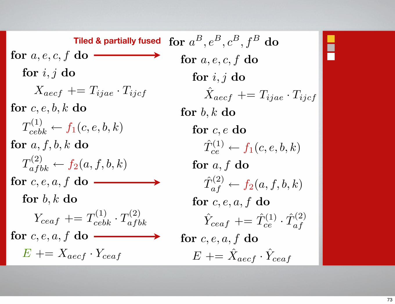
for a, e, c, f dofor i, j do
Xaecf += Tijae · Tijcf
for c, e, b, k do
T (1)cebk ← f1(c, e, b, k)
for a, f, b, k do
T (2)afbk ← f2(a, f, b, k)
for c, e, a, f dofor b, k do
Yceaf += T (1)cebk · T (2)
afbk
for c, e, a, f doE += Xaecf · Yceaf
Tiled & partially fused for aB , eB , cB , fB dofor a, e, c, f do
for i, j doXaecf += Tijae · Tijcf
for b, k dofor c, e do
T (1)ce ← f1(c, e, b, k)
for a, f do
T (2)af ← f2(a, f, b, k)
for c, e, a, f do
Yceaf += T (1)ce · T (2)
af
for c, e, a, f doE += Xaecf · Yceaf
73
74

75

Next time:Empirical compilers and tools
76

“In conclusion…”
77

Backup slides
78
Recommended