
Rochester Institute of Technology Rochester Institute of Technology
RIT Scholar Works RIT Scholar Works
Theses
4-2021
Automatic Speech Recognition for Low-Resource and Automatic Speech Recognition for Low-Resource and
Morphologically Complex Languages Morphologically Complex Languages
Ethan Morris [email protected]
Follow this and additional works at: https://scholarworks.rit.edu/theses
Recommended Citation Recommended Citation Morris, Ethan, "Automatic Speech Recognition for Low-Resource and Morphologically Complex Languages" (2021). Thesis. Rochester Institute of Technology. Accessed from
This Thesis is brought to you for free and open access by RIT Scholar Works. It has been accepted for inclusion in Theses by an authorized administrator of RIT Scholar Works. For more information, please contact [email protected].
Automatic Speech Recognition for Low-Resourceand Morphologically Complex Languages
Ethan Morris
Automatic Speech Recognition for Low-Resourceand Morphologically Complex Languages
Ethan MorrisApril 2021
A Thesis Submittedin Partial Fulfillment
of the Requirements for the Degree ofMaster of Science
inComputer Engineering
Department of Computer Engineering
Automatic Speech Recognition for Low-Resourceand Morphologically Complex Languages
Ethan Morris
Committee Approval:
Emily Prud’hommeaux Advisor DateDepartment of Computer Science, Boston College
Alexander Loui DateDepartment of Computer Engineering
Andreas Savakis DateDepartment of Computer Engineering
i
Acknowledgments
I would like to thank Dr. Emily Prud’hommeaux for her continued support and
guidance, with invaluable suggestions. I am also thankful for Dr. Alexander Loui
and Dr. Andreas Savakis for being on the thesis committee. I also wish to thank
Dr. Raymond Ptucha, Dr. Christopher Homan, and Robert Jimerson for their ideas,
advice, and general expertise.
ii

Abstract
The application of deep neural networks to the task of acoustic modeling for au-
tomatic speech recognition (ASR) has resulted in dramatic decreases of word error
rates, allowing for the use of this technology in smart phones and personal home
assistants in high-resource languages. Developing ASR models of this caliber, how-
ever, requires hundreds or thousands of hours of transcribed speech recordings, which
presents challenges for most of the world’s languages. In this work, we investigate the
applicability of three distinct architectures that have previously been used for ASR
in languages with limited training resources. We tested these architectures using
publicly available ASR datasets for several typologically and orthographically diverse
languages, whose data was produced under a variety of conditions using different
speech collection strategies, practices, and equipment. Additionally, we performed
data augmentation on this audio, such that the amount of data could increase nearly
tenfold, synthetically creating higher resource training. The architectures and their
individual components were modified, and parameters explored such that we might
find a best-fit combination of features and modeling schemas to fit a specific language
morphology. Our results point to the importance of considering language-specific and
corpus-specific factors and experimenting with multiple approaches when developing
ASR systems for resource-constrained languages.
iii
Contents
Signature Sheet i
Acknowledgments ii
Abstract iii
Table of Contents iv
List of Figures vii
List of Tables viii
1 Introduction and Motivation 1
1.1 Introduction and Motivation . . . . . . . . . . . . . . . . . . . . . . . 1
1.2 Document Structure . . . . . . . . . . . . . . . . . . . . . . . . . . . 2
2 Background 4
2.1 Introduction . . . . . . . . . . . . . . . . . . . . . . . . . . . . . . . . 4
2.2 Automatic Speech Recognition . . . . . . . . . . . . . . . . . . . . . . 4
2.3 Feature Extraction . . . . . . . . . . . . . . . . . . . . . . . . . . . . 5
2.3.1 Spectral Features . . . . . . . . . . . . . . . . . . . . . . . . . 6
2.3.2 Mel Filterbanks . . . . . . . . . . . . . . . . . . . . . . . . . . 7
2.3.3 Mel-frequency Cepstral Coefficients (MFCCs) . . . . . . . . . 7
2.3.4 Feature Space Maximum Likelihood Linear Regression (fMLLR) 8
2.3.5 I/X Vector . . . . . . . . . . . . . . . . . . . . . . . . . . . . . 8
2.4 Acoustic Models . . . . . . . . . . . . . . . . . . . . . . . . . . . . . . 9
2.4.1 Hidden Markov Model . . . . . . . . . . . . . . . . . . . . . . 9
2.4.2 Gaussian Mixture Model . . . . . . . . . . . . . . . . . . . . . 9
2.4.3 Deep Neural Network . . . . . . . . . . . . . . . . . . . . . . . 10
2.4.4 Recurrent Neural Networks . . . . . . . . . . . . . . . . . . . 11
2.5 Language Models . . . . . . . . . . . . . . . . . . . . . . . . . . . . . 12
2.5.1 N-Gram . . . . . . . . . . . . . . . . . . . . . . . . . . . . . . 12
2.5.2 Neural . . . . . . . . . . . . . . . . . . . . . . . . . . . . . . . 12
2.5.3 Trans-dimensional Random Field (TRF) . . . . . . . . . . . . 13
2.6 Data Augmentation . . . . . . . . . . . . . . . . . . . . . . . . . . . . 13
iv
CONTENTS
2.6.1 Pitch/Speed/Noise . . . . . . . . . . . . . . . . . . . . . . . . 13
2.6.2 SpecAugment . . . . . . . . . . . . . . . . . . . . . . . . . . . 14
2.6.3 Speech Synthesis . . . . . . . . . . . . . . . . . . . . . . . . . 15
2.7 Evaluation Metrics . . . . . . . . . . . . . . . . . . . . . . . . . . . . 16
2.7.1 Character/Word Error Rate . . . . . . . . . . . . . . . . . . . 16
2.7.2 Perplexity . . . . . . . . . . . . . . . . . . . . . . . . . . . . . 17
2.8 Frameworks . . . . . . . . . . . . . . . . . . . . . . . . . . . . . . . . 17
2.8.1 Kaldi . . . . . . . . . . . . . . . . . . . . . . . . . . . . . . . . 17
2.8.2 DeepSpeech . . . . . . . . . . . . . . . . . . . . . . . . . . . . 18
2.8.3 Wav2Letter/Wav2Vec . . . . . . . . . . . . . . . . . . . . . . 18
2.8.4 WireNet . . . . . . . . . . . . . . . . . . . . . . . . . . . . . . 19
3 Datasets 21
3.1 Amharic . . . . . . . . . . . . . . . . . . . . . . . . . . . . . . . . . . 21
3.1.1 Language Description . . . . . . . . . . . . . . . . . . . . . . . 21
3.1.2 Prior ASR Work . . . . . . . . . . . . . . . . . . . . . . . . . 22
3.2 Bemba . . . . . . . . . . . . . . . . . . . . . . . . . . . . . . . . . . . 23
3.2.1 Language Description . . . . . . . . . . . . . . . . . . . . . . . 23
3.2.2 Prior ASR Work . . . . . . . . . . . . . . . . . . . . . . . . . 23
3.3 Iban . . . . . . . . . . . . . . . . . . . . . . . . . . . . . . . . . . . . 24
3.3.1 Language Description . . . . . . . . . . . . . . . . . . . . . . . 24
3.3.2 Prior ASR Work . . . . . . . . . . . . . . . . . . . . . . . . . 25
3.4 Seneca . . . . . . . . . . . . . . . . . . . . . . . . . . . . . . . . . . . 25
3.4.1 Language Description . . . . . . . . . . . . . . . . . . . . . . . 25
3.4.2 Prior ASR Work . . . . . . . . . . . . . . . . . . . . . . . . . 26
3.5 Swahili . . . . . . . . . . . . . . . . . . . . . . . . . . . . . . . . . . . 26
3.5.1 Language Description . . . . . . . . . . . . . . . . . . . . . . . 26
3.5.2 Prior ASR Work . . . . . . . . . . . . . . . . . . . . . . . . . 27
3.6 Vietnamese . . . . . . . . . . . . . . . . . . . . . . . . . . . . . . . . 27
3.6.1 Language Description . . . . . . . . . . . . . . . . . . . . . . . 27
3.6.2 Prior ASR Work . . . . . . . . . . . . . . . . . . . . . . . . . 28
3.7 Wolof . . . . . . . . . . . . . . . . . . . . . . . . . . . . . . . . . . . 28
3.7.1 Language Description . . . . . . . . . . . . . . . . . . . . . . . 28
3.7.2 Prior ASR Work . . . . . . . . . . . . . . . . . . . . . . . . . 29
v

CONTENTS
4 Methodology 30
4.1 Language Comparison . . . . . . . . . . . . . . . . . . . . . . . . . . 30
4.1.1 Average Utterance Length . . . . . . . . . . . . . . . . . . . . 30
4.1.2 Quality Measures . . . . . . . . . . . . . . . . . . . . . . . . . 30
4.2 Kaldi . . . . . . . . . . . . . . . . . . . . . . . . . . . . . . . . . . . . 32
4.3 WireNet . . . . . . . . . . . . . . . . . . . . . . . . . . . . . . . . . . 33
4.3.1 Transfer Learning . . . . . . . . . . . . . . . . . . . . . . . . . 33
4.3.2 Data Augmentation . . . . . . . . . . . . . . . . . . . . . . . . 33
4.3.3 Architecture Exploration . . . . . . . . . . . . . . . . . . . . . 34
4.3.4 Feature Comparison . . . . . . . . . . . . . . . . . . . . . . . 35
4.4 Speaker Re-partitioning . . . . . . . . . . . . . . . . . . . . . . . . . 36
4.5 Language Model Exploration . . . . . . . . . . . . . . . . . . . . . . . 36
5 Results 37
5.1 Kaldi Results . . . . . . . . . . . . . . . . . . . . . . . . . . . . . . . 37
5.1.1 Overall . . . . . . . . . . . . . . . . . . . . . . . . . . . . . . . 37
5.1.2 Data Augmentation . . . . . . . . . . . . . . . . . . . . . . . . 38
5.2 WireNet . . . . . . . . . . . . . . . . . . . . . . . . . . . . . . . . . . 39
5.2.1 Overall Results . . . . . . . . . . . . . . . . . . . . . . . . . . 39
5.2.2 Architecture Exploration . . . . . . . . . . . . . . . . . . . . . 39
5.2.3 Transfer Learning . . . . . . . . . . . . . . . . . . . . . . . . . 43
5.2.4 Feature Comparison . . . . . . . . . . . . . . . . . . . . . . . 44
5.3 Language Comparison . . . . . . . . . . . . . . . . . . . . . . . . . . 46
5.4 Language Model Exploration . . . . . . . . . . . . . . . . . . . . . . . 48
5.5 Speaker Overlap . . . . . . . . . . . . . . . . . . . . . . . . . . . . . . 48
6 Conclusions 56
6.1 Conclusions . . . . . . . . . . . . . . . . . . . . . . . . . . . . . . . . 56
6.2 Future Work . . . . . . . . . . . . . . . . . . . . . . . . . . . . . . . . 57
Bibliography 58
vi
List of Figures
2.1 Generic pipeline of an ASR system. . . . . . . . . . . . . . . . . . . . 4
2.2 An overview of the most basic feature extraction process, including the
different stopping points for various features [1]. . . . . . . . . . . . . 6
2.3 Augmentations applied to the base input, given at the top. From
top to bottom, the figures depict the log mel spectrogram of the base
input with no augmentation, time warp, frequency masking and time
masking applied [2] . . . . . . . . . . . . . . . . . . . . . . . . . . . . 15
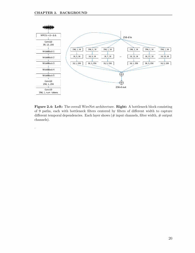
2.4 Left: The overall WireNet architecture. Right: A bottleneck block
consisting of 9 paths, each with bottleneck filters centered by filters of
different width to capture different temporal dependencies. Each layer
shows (# input channels, filter width, # output channels). . . . . . . 20
4.1 Comparison of the WADA SNR algorithm and the average estimated
NIST SNR against an artificially corrupted database. [3] . . . . . . . 32
5.1 CER vs. training epochs of the Swahili language at specific bottleneck
depths. . . . . . . . . . . . . . . . . . . . . . . . . . . . . . . . . . . . 41
5.2 U-Net architecture where the convolutional size increases to a maxi-
mum of 1024, before reducing back to the input size. [4] . . . . . . . 42
5.3 CER vs. training epochs through the stages of training the Swahili
language with transfer learning. . . . . . . . . . . . . . . . . . . . . . 43
5.4 CER vs. training epochs through the stages of training the Swahili
language without transfer learning. . . . . . . . . . . . . . . . . . . . 44
5.5 Best produced WER vs. NIST SNR across all languages, training set
depicted. . . . . . . . . . . . . . . . . . . . . . . . . . . . . . . . . . . 47
5.6 Best produced WER vs. WADA SNR across all languages, training set
depicted. . . . . . . . . . . . . . . . . . . . . . . . . . . . . . . . . . . 47
5.7 WER vs. % of Test Set for the Bemba Language. . . . . . . . . . . . 51
5.8 WER vs. % of Test Set for the Seneca Language. . . . . . . . . . . . 53
5.9 WER vs. % of Test Set for the Wolof Language. . . . . . . . . . . . . 55
vii
List of Tables
3.1 Amharic Dataset Information . . . . . . . . . . . . . . . . . . . . . . 22
3.2 Bemba Dataset Information . . . . . . . . . . . . . . . . . . . . . . . 23
3.3 Iban Dataset Information . . . . . . . . . . . . . . . . . . . . . . . . 24
3.4 Seneca Dataset Information . . . . . . . . . . . . . . . . . . . . . . . 26
3.5 Swahili Dataset Information . . . . . . . . . . . . . . . . . . . . . . . 27
3.6 Vietnamese Dataset Information . . . . . . . . . . . . . . . . . . . . . 28
3.7 Wolof Dataset Information . . . . . . . . . . . . . . . . . . . . . . . . 29
5.1 Overall Kaldi results for the two best architectures across all languages. 37
5.2 Kaldi results for the two best architectures across the Wolof language
with data augmentation. . . . . . . . . . . . . . . . . . . . . . . . . . 38
5.3 Overall WireNet results across all languages. . . . . . . . . . . . . . . 39
5.4 WireNet architecture exploration for Swahili, varying the width and
depth of the system. . . . . . . . . . . . . . . . . . . . . . . . . . . . 40
5.5 WireNet results for the Swahili language with U-Net styled architecture. 42
5.6 Feature Comparison of Languages . . . . . . . . . . . . . . . . . . . . 45
5.7 Feature Comparison of Wolof . . . . . . . . . . . . . . . . . . . . . . 45
5.8 SNR overview per language. . . . . . . . . . . . . . . . . . . . . . . . 46
5.9 Neural language model perplexity for the language of Wolof. . . . . . 48
5.10 Word error rate (WER) for each language under the three architectures
and two train/test split settings: the original, in which no speaker has
utterances in both the train and test sets (Disjoint), and a new split
in which each speaker’s utterances are split between the training and
test sets (Overlap). . . . . . . . . . . . . . . . . . . . . . . . . . . . . 49
5.11 Determining the impact of holding out each speaker for the Bemba
language. . . . . . . . . . . . . . . . . . . . . . . . . . . . . . . . . . 50
5.12 Determining the impact of holding out each speaker for the Seneca
language. . . . . . . . . . . . . . . . . . . . . . . . . . . . . . . . . . 52
5.13 Determining the impact of holding out each speaker for the Wolof
language. . . . . . . . . . . . . . . . . . . . . . . . . . . . . . . . . . 54
viii

Chapter 1
Introduction and Motivation
1.1 Introduction and Motivation
Automatic speech recognition (ASR) is the process by which audio input is taken
and transcribed to text, for use in many modern technologies such as Amazon’s
Alexa, Google Assistant, or Apple’s Siri. The ability to accurately detect and convert
these spoken words into linguistic data is quite lucrative and sought after by large
corporations for use in product development, as the spoken word is roughly 3 times
faster than keyboard input [5]. The realm of speech recognition and transcription
has been explored for over 60 years and is just recently being converted to the deep
learning realm from the traditional statistical based models. This switch allows for
the traditional deep learning architectures and design processes to take place, with
revolutions occurring every few years as companies develop new, application specific
models. However, these ASR pipelines require hundreds, if not thousands, of hours
of data [2, 6]; a corpus of this size does not exist for a large majority of the 7,117
languages, especially as over 40% are endangered, with less than 1,000 speakers [7].
In addition to the shear amount of raw audio data necessary for prediction, a large
collection of written text must be available for appropriate constraint and correction
of this output - another limiting factor.
These existing architectures can be adapted to a low-resource setting using tech-
1
CHAPTER 1. INTRODUCTION AND MOTIVATION
niques such as transfer learning and data augmentation, but challenges remain. Not
every implementation, pipeline, or weighted staging will fit the characteristics of a
target language. As such, the motivation of this thesis is to expand upon the current
deep learning implementations of low-resource speech recognition [8, 9, 10] through
a study against small and diverse ASR training corpora. The final result will be a
pipeline capable of accepting an under-resourced language, determining the appro-
priate model parameters based on the based on the features of the language and the
corpus, such as morphological complexity, orthographic system, speaker diversity, and
recording quality, and producing character-based transcriptions from the input data.
Specifically, the principal contributions of this thesis are outlined as follows:
• Examine the diverse field of current automatic speech recognition technologies
and evaluate their effectiveness across several diverse languages.
• Input feature comparison for language size and morphologies.
• State of the art convolutional model architecture optimization.
• Purposeful dataset re-partitioning to remove the natural disjoint speaker im-
plementations.
1.2 Document Structure
The remainder of this document is organized as follows:
• Chapter 2 reviews the background of ASR, including feature extraction, model
types, and related works.
• Chapter 3 breaks down the language corpora used in this thesis.
• Chapter 4 describes the methodology and approach towards developing a novel
low resource language transcriber.
2

CHAPTER 1. INTRODUCTION AND MOTIVATION
• Chapter 5 outlines the experimental results and performance across languages.
• Chapter 6 summarizes the key concepts and diagrams potential future work.
3
Chapter 2
Background
2.1 Introduction
This chapter describes the basics of ASR, deep learning construction, and prior work.
2.2 Automatic Speech Recognition
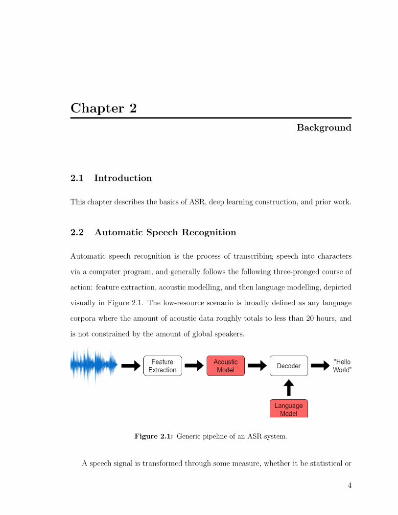
Automatic speech recognition is the process of transcribing speech into characters
via a computer program, and generally follows the following three-pronged course of
action: feature extraction, acoustic modelling, and then language modelling, depicted
visually in Figure 2.1. The low-resource scenario is broadly defined as any language
corpora where the amount of acoustic data roughly totals to less than 20 hours, and
is not constrained by the amount of global speakers.
Figure 2.1: Generic pipeline of an ASR system.
A speech signal is transformed through some measure, whether it be statistical or
4

CHAPTER 2. BACKGROUND
deep learning, into a small window of time meant to capture into a small window of
time with stable acoustic properties that more easily be associated with an individual
speech sound, or phoneme. This is then passed into an acoustic model, Gaussian
Mixture Model (GMM), Deep Neural Network (DNN), etc., which generally uses some
sort of mechanism to capture temporal data, before predicting a character/sequence
of characters. A decoder, in most cases relying on a language model that models
likely words and word sequences, is then applied to make sure that this prediction
is a valid combination of characters for the language and is likely to occur; this final
result is then output to the user.
2.3 Feature Extraction
In deep learning, this raw wave form may be passed directly into the deep learning
model [11, 12, 13, 14], however these systems produce marginally worse (1-2%) results
as opposed to using hand-crafted features. These hand-crafted features aim to emulate
the brain’s auditory response to sound, and although there are concerns they may
hinder speaker characteristic extraction [12], traditional state-of-the-art methods [15,
16] seem unhindered. Additionally, research is being conducted into making these
hand-crafted features [17], more capable of aptly capturing speaker embeddings. An
overview of the most basic pre-processing techniques is shown in Figure 2.2.
5

CHAPTER 2. BACKGROUND
Figure 2.2: An overview of the most basic feature extraction process, including the dif-ferent stopping points for various features [1].
2.3.1 Spectral Features
The most basic features are meant to visualize the short time power spectrum, which
contains data about the vocal tract and are meant to depict human speech perception.
First, DC offset removal and pre-emphasis is applied due to the rapid decay of an
audio signal. This boosts the energy of the signal, emphasizing the higher frequency
components which are more likely to contain speech. Next, these features are divided
into small time-scale data, to attempt to capture a morpheme; typically, a value of
20-40 ms is used. A window function, generally Hamming, is applied to taper the
frames as opposed to harsh segmentation, allowing for the potential capture across
6

CHAPTER 2. BACKGROUND
multiple frames. This data is converted into several discrete frequencies via a Fourier
transform, to determine the spectral density of the audio. Often such information
is too finely calculated when compared to the data interpreted by the human ear;
therefore, data is grouped at certain frequencies, calculated via the sampling rate, to
emphasize the frequencies not at the extrema.
Before additional filtering is applied, the features can be extracted at this stage:
the spectral coefficients. These are not often used, as the filtering stages remove
frequencies unperceived by humans, but in systems where less modified data is desired
[18] they can produce quality results.
2.3.2 Mel Filterbanks
Mel filtering occurs via the following Equation 2.1 and was introduced by Stevens
and Volkmann [19] as a way to mimic the way human speech perception attends to
specific frequency bands.
mel(f) = 1127 ∗ ln(1 +f
700) (2.1)
Additionally, the natural logarithm can be applied again, further normalizing the
filterbanks left in a highly correlated fashion; referred to as logmel filterbanks. This
data can be used as an input to the system in the hopes of maintaining the highly
correlated temporal information in the deep learning model.
2.3.3 Mel-frequency Cepstral Coefficients (MFCCs)
The final calculation is to take the discrete cosine of these log energies to decorrelate
these overlapping values [20, 21].
These features themselves carry no time-based information and in the speech
realm, adding the delta coefficients, allow the system to model some temporal infor-
mation in a time independent situation. The order of the MFCCs is determined to
7

CHAPTER 2. BACKGROUND
be 12 with 1 measure of overall energy, as additional orders determined not helpful
in ASR applications [20].
2.3.4 Feature Space Maximum Likelihood Linear Regression (fMLLR)
One important notion to consider when building deep learning systems is overfitting
to the training data. In images this can occur with respect to the background, and in
audio with respect to the speaker themself. Thus, speaker normalization is considered
to minimize the potential of overfitting to a speaker’s audio characteristics. This is
accomplished through Maximum Likelihood Linear Regression (MLLR), where the
means of the Gaussian are transformed via the average of the feature, where the
estimators are produced based on this likelihood [22].
FMLLR is a constrained MLLR, meaning it is calculated in a similar manner,
except including an extended transformation matrix and observation vector, and ap-
plying the transformation on the variance as opposed to the mean [23].
2.3.5 I/X Vector
I-Vectors are information taken from a Gaussian Mixture Model (GMM) system which
has been trained on the full corpus. In the GMM space, no distinctions are made
between speaker and channel effects, thus assuming that every utterance has been
produced by a new speaker [24]. Then, with Principal Component Analysis (PCA)
and normalization, i-vectors are extracted per speaker. These i-vectors are extracted,
and their dimension reduced via Linear Discriminant Analysis (LDA), before able to
be used as inputs [25] to the deep learning model.
X-Vectors are similar in nature to i-vectors, except taken from a deep neural
network (DNN) that is trained to discriminate between speakers. This DNN takes
in filterbanks and classifies speakers based on this data; x-vectors are extracted from
a convolutional layer before dimensional reduction occurs within the neural network
8

CHAPTER 2. BACKGROUND
layers [26, 17]. In a Cantonese ASR system, these x-vectors were able to produce 2-3%
equal error-rate (EER) reductions as opposed to i-vector based systems but require
an additional training step to produce the input data.
2.4 Acoustic Models
Over time, two main categories of models have risen to prominence, statistical and
deep learning, with their derivatives producing nearly every state-of-the-art result.
2.4.1 Hidden Markov Model
A Markov model is a finite-state system where the behavior depends on the current
state as a method of predicting the next state. Whenever the state transition infor-
mation is not directly evident or the states are not observable, this is referred to as
a Hidden Markov Model (HMM). Speech is temporally dependent, which HMMs are
able to model through self-loops, and predict the speech, typically via the Viterbi
or some dynamic programming algorithm, to find the most likely next character or
phone. The forward and backward algorithms are used to update the internal proba-
bilities of each state transition, allowing for the HMM to update the internal weights,
similar to propagation in a DNN. Referred to as the EM step, the parameters can
be easily iterated and increase the internal state of the HMM’s convergence rate [27].
Models for sentences can be formed through the concatenation of the phone HMMs,
allowing the prediction of a string of phones [28].
2.4.2 Gaussian Mixture Model
Gaussian mixture models (GMM) systems are combined alongside the HMM to es-
timate the density and maximum the likelihood of the data’s distribution. If the
weights are allowed to vary slightly in the subspace, but share a global mapping,
this is referred to as a Subspace Gaussian Mixture Model (SGMM) [29]. Subspaces
9
CHAPTER 2. BACKGROUND
are introduced as opposed towards using larger models as a means of reducing the
number of parameter estimation issues by reducing the dimensionality of the system
[30].
Although capable of producing high quality results, the noted issue with GMMs
is that they are inefficient at modeling non-linear data [31]. Thus, speech, with its
inflection, tone, and other properties are not the ideal application.
2.4.3 Deep Neural Network
Deep neural networks are incredibly prevalent in industry applications as a method of
classification and recognition. Through the stacking of hidden layers on large amounts
of data, better predictions can be made on the non-linear data as there is no concept of
spatial representation. Each hidden layer uses an activation function, often a Rectified
Linear Unit (ReLU), to map the weights to a standardized state. For multiclass
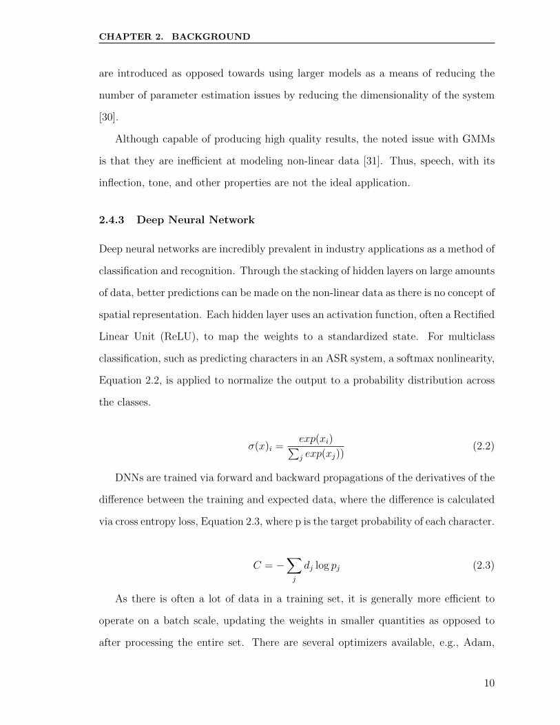
classification, such as predicting characters in an ASR system, a softmax nonlinearity,
Equation 2.2, is applied to normalize the output to a probability distribution across
the classes.
σ(x)i =exp(xi)∑j exp(xj))
(2.2)
DNNs are trained via forward and backward propagations of the derivatives of the
difference between the training and expected data, where the difference is calculated
via cross entropy loss, Equation 2.3, where p is the target probability of each character.
C = −∑j
dj log pj (2.3)
As there is often a lot of data in a training set, it is generally more efficient to
operate on a batch scale, updating the weights in smaller quantities as opposed to
after processing the entire set. There are several optimizers available, e.g., Adam,
10

CHAPTER 2. BACKGROUND
Stochastic Gradient Descent (SGD), etc., which smooth the gradient per batch such
that large jumps do not occur too quickly, proportionally introducing these updated
weights.
DNNs with many hidden layers can take thousands of iterations to optimize suc-
cessfully [32]; therefore, often weight initialization is applied through methods like
unsupervised pre-training [33] or transfer learning [34], such that the backward prop-
agation magnitudes are not incredibly large.
As speech is incredibly time dependent, something with which traditional convo-
lutional neural networks do not bother, architectures have been proposed that modify
these convolutional constructions to include a concept called Attention [35] by relat-
ing the positions of a sequence to compute its entire representation. Through this
concept, offshoots of the traditional DNN can be created, notably the Transformer
model.
2.4.4 Recurrent Neural Networks
The drawback of DNNs is that they require a fixed dimensionality vector and for
sequential data, a conglomerate mapping of these sequences is not entirely feasible in
a generic sense. As such, architectures have arisen, called Long-Short Term Memory
(LSTM) and Recurrent Neural Networks (RNNs) [36, 37] which specialize in modeling
the data per timestep. These can be incredibly effective at predicting speech when
there is lots of input data available [38] but are notoriously difficult to train [39]
due to the long-range dependencies and vanishing and exploding gradient problems
during propagation. Modern RNN and LSTM networks are capable of producing
quality results [40], but still require thousands of hours of data and are not capable
of beating DNNs in the low-resource environment [41].
11
CHAPTER 2. BACKGROUND
2.5 Language Models
Whatever model implemented, whether it be statistical or deep learning based, it
will output a string of characters or words that it feels best fits the audio signal.
This information, by itself, is often inaccurate due to the similarity between phone
pronunciation, especially given the speaker variability. A language model is used to
convert this data into a more realistic sequences via rescoring the prediction based on
a corpus of text from the language of choice. Language models analyze the textual
data and estimate the probability of a word sequence occurring; thus, can replace
predictive words with what the language model has seen more commonly in the data.
2.5.1 N-Gram
The typical language model used is an n-gram type, where n is between 1 and 5. In
this case n refers to the depth of the probability search, looking n - 1 words back.
The probability is calculated via the chain rule and maximum likelihood estimate for
every word in the corpus, thus predicting the next most common word following a
specific word or sequence of words [42].
2.5.2 Neural
The n-gram model is successful but falls victim to the curse of dimensionality past n=5
as the number of words it must keep track of grows significantly, with little reduction
in the predictive ability. Long short-term memory (LSTM) language models are
able to capture the long-term information more efficiently than n-gram models, and
although the calculation of the probability takes longer, the predictive ability is better
because of the infinite history states [43]. Recurrent neural networks (RNN) can also
be used for this task, but the context range is more limited due to the vanishing
gradient problem.
12
CHAPTER 2. BACKGROUND
2.5.3 Trans-dimensional Random Field (TRF)
There is a third explored language model, the trans-dimensional random field model.
By mixing a collection of random fields in different dimensions, allowing for larger
width and depth of the data connectivity [11]. These models learn through stochastic
approximation and perform a similar Markov updating sequence as in the HMM
systems. These are an interesting application of non-deep learning language modeling,
but do not produce equivalent rates to the LSTM LM.
2.6 Data Augmentation
2.6.1 Pitch/Speed/Noise
Most of the ASR architecture work proceeds with hundreds or thousands of hours of
audio data but collecting speech corpora of this size is time-consuming and expensive.
As a result, available speech corpora for many languages have fewer than 20 hours of
transcribed audio suitable for acoustic model training. In these cases, we can modify
the data using traditional acoustic methods, such as the Pitch-Synchronous Overlap-
Add (PSOLA) [44, 45] approach for pitch shifting directly in the time domain, which
keeps the original audio’s tempo, adjusting the timbre.
Additionally, time-stretching [46] can be applied to make the original audio sound
as if it were spoken at a different tempo, maintaining the original timbre. Traditional
methods include Waveform Similarity Overlapp-Add (WSOLA) and phase vocoder,
with the note of caution that a reduction of artifacts can be introduced when modi-
fying the original audio.
Lastly, noise additions, e.g., fan, barking, etc. can be incorporated into the audio
data [47] as a method of artificially generating new training data. However, research
into noise robust systems have concluded that some methods such as Wiener filtering
and spectral subtraction are satisfactory at compensating the features for this noise
13
CHAPTER 2. BACKGROUND
and deep, wide hidden layers of a DNN naturally normalize heterogenous data [48].
Therefore, it may be substantially less beneficial to introduce these elements of noise
as opposed to traditional music based alterations in the training set, because of the
duplication of audio. It still may be favorable for the overall system if noise were
introduced into the test set to reduce overfitting.
2.6.2 SpecAugment
In addition to the time-domain based mutations, frequency-domain based masks can
be applied to the audio signal to introduce regularization and helps the network
emphasize robustness. These methods are referred to as time and frequency masking
[2], where consecutive time steps or frequency bands are nulled out, depicted in Figure
2.3, to add this element of regularization.
14

CHAPTER 2. BACKGROUND
Figure 2.3: Augmentations applied to the base input, given at the top. From top tobottom, the figures depict the log mel spectrogram of the base input with no augmentation,time warp, frequency masking and time masking applied [2]
.
2.6.3 Speech Synthesis
In a low-resource setting, the ability to generate data that may be for the training
process is invaluable. Providing the model with additional data in a data-dependent
environment allows for a better opportunity at a higher classification rate.
2.6.3.1 Tacotron
Tacotron 2 is a neural network architecture that allows for the speech synthesis of
textual data. Using mel spectrograms and an encoder/decoder network, the weights
are learned before using a WaveNet Vocoder to produce the waveforms [49]. This
is an incredibly deep network and the number of iterations required for successful
15
CHAPTER 2. BACKGROUND
synthesis on a large dataset is quite high; although, studies have reproduced quality
synthetic data with a small training set of 1 hour and fewer [50], the training time
and resources required is still large.
2.6.3.2 Festival
Festival [51] and its subsidiaries is the most popular non-neural speech synthesis, using
statistical parametric speech synthesis and back ended by HMMs. Similar to language
models, the non-neural performance is not as effective at producing indistinguishable
synthesized speech; however, the speed and efficiency of this implementation implies
a suitable alternative.
2.7 Evaluation Metrics
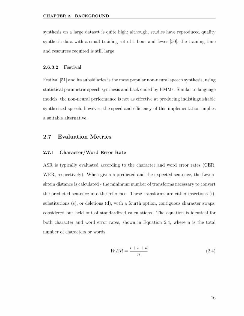
2.7.1 Character/Word Error Rate
ASR is typically evaluated according to the character and word error rates (CER,
WER, respectively). When given a predicted and the expected sentence, the Leven-
shtein distance is calculated - the minimum number of transforms necessary to convert
the predicted sentence into the reference. These transforms are either insertions (i),
substitutions (s), or deletions (d), with a fourth option, contiguous character swaps,
considered but held out of standardized calculations. The equation is identical for
both character and word error rates, shown in Equation 2.4, where n is the total
number of characters or words.
WER =i+ s+ d
n(2.4)
16
CHAPTER 2. BACKGROUND
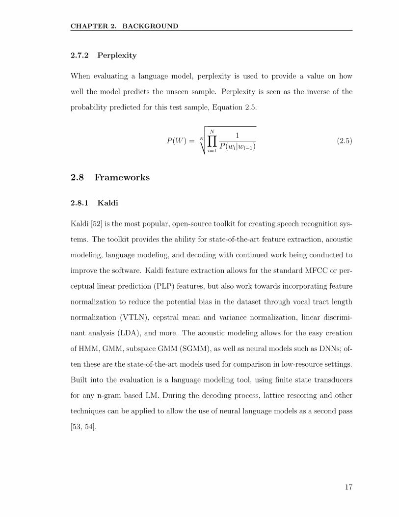
2.7.2 Perplexity
When evaluating a language model, perplexity is used to provide a value on how
well the model predicts the unseen sample. Perplexity is seen as the inverse of the
probability predicted for this test sample, Equation 2.5.
P (W ) = N
√√√√ N∏i=1
1
P (wi|wi−1)(2.5)
2.8 Frameworks
2.8.1 Kaldi
Kaldi [52] is the most popular, open-source toolkit for creating speech recognition sys-
tems. The toolkit provides the ability for state-of-the-art feature extraction, acoustic
modeling, language modeling, and decoding with continued work being conducted to
improve the software. Kaldi feature extraction allows for the standard MFCC or per-
ceptual linear prediction (PLP) features, but also work towards incorporating feature
normalization to reduce the potential bias in the dataset through vocal tract length
normalization (VTLN), cepstral mean and variance normalization, linear discrimi-
nant analysis (LDA), and more. The acoustic modeling allows for the easy creation
of HMM, GMM, subspace GMM (SGMM), as well as neural models such as DNNs; of-
ten these are the state-of-the-art models used for comparison in low-resource settings.
Built into the evaluation is a language modeling tool, using finite state transducers
for any n-gram based LM. During the decoding process, lattice rescoring and other
techniques can be applied to allow the use of neural language models as a second pass
[53, 54].
17

CHAPTER 2. BACKGROUND
2.8.2 DeepSpeech
DeepSpeech [15, 55] is an RNN based decoder system which produced state-of-the-art
results that have now been superseded. The techniques used still provide valuable
insight into methodology that can be beneficial in a low-resource environment. Their
use of data augmentation, inducing noise and inflecting the pitch, is pivotal in the
low resource environment. Additionally, their use of a bidirectional RNN, paired
with Connectionist Temporal Classification (CTC) aligns the transcription with the
audio [15], reducing potential silence and shortening the waveform. The DeepSpeech
experiments required 11,940 hours of English data or 9,400 hours of Mandarin and
required weeks of training time; this highlights the inability to apply RNNs to a
low-resource scenario.
2.8.3 Wav2Letter/Wav2Vec
Wav2Letter [9, 56] provides a one-pass beam-search decoder with thresholding, prun-
ing, and smearing capabilities for maximizing n-gram probabilities. The model archi-
tecture itself is a 12-layer convolutional neural network with incredibly large, fixed
widths associated per layer, introducing training overhead. Such a model was capable
of competitive results against standard corpora, but does not produce state-of-the-art.
Wav2Vec [57, 14] introduces feature encoder and transformer models to take in
the raw audio input, learn the appropriate features, contextualize the data, before
outputting the results. Unsupervised learning is first applied to the language, where
discrete speech units [58] are first learned via a gumbel-softmax, before being passed
into a multi-layer convolutional neural network as a means of audio encoding. These
representations are passed into a Transformer network, quantized, and transformed
into the final result via contrastive predictive coding [59]. Facebook does indicate
state-of-the-art results on low-resource test sets of 10 minutes, 1 hour, and 10 hours;
the key being unsupervised learning on a large dataset (960 hours) of the same lan-
18

CHAPTER 2. BACKGROUND
guage, before finetuning on the small, labeled dataset, as well as using a transformer-
based language model for decoding. These results likely will not generalize to the
low-resource scenario where such an unsupervised learning schema can occur.
2.8.4 WireNet
WireNet [60] is a novel fully convolutional ASR architecture distinct from the other
toolkits described prior and was developed specifically for the under-resourced lan-
guage of Seneca, Figure 2.4. The architecture and associated training pipeline pro-
duced substantially lower word error rates for a 10-hour Seneca corpus than both
DeepSpeech, trained using a transfer learning and data augmentation pipeline, and
the most widely used architectures available in Kaldi. The main architectural feature
is a stack of Inception [61] and ResNet [62] styled bottleneck blocks, with wide filter
widths that emulate the temporal nature of audio. A multi-staged pipeline was em-
ployed with transfer learning from a high-resource language, transitioning into heavily
augmented training data, before fine-tuning on the original, unaugmented data. This
learning strategy allows for the neural network’s weights to be better initialized as
the network can use the larger datasets to converge more quickly, before being refined
on the original, smaller dataset.
19
CHAPTER 2. BACKGROUND
Figure 2.4: Left: The overall WireNet architecture. Right: A bottleneck block consistingof 9 paths, each with bottleneck filters centered by filters of different width to capturedifferent temporal dependencies. Each layer shows (# input channels, filter width, # outputchannels).
.
20
Chapter 3
Datasets
3.1 Amharic
3.1.1 Language Description
The Amharic (ISO 693-3 amh) language is a member of the Semitic branch of the
Afro-Asiatic language family spoken by approximately 25 million people, primarily
in Ethiopia. The Amharic writing system is based on the Ge’ez script, referred to as
fidal, and each symbol represents the combination of a character and a vowel, known
as a CV syllable. Thus, the script consists of 231 distinct CV syllables, where words
are formed via a root-pattern morphology, where affixes influence word construction.
There are 38 phonemes, 31 consonants and 7 vowels, and are classified into the groups:
stops, fricatives, nasals, liquids, and semivowels. The corpus [16] was collected in a
closed environment via read speech from 124 native speakers, 70 male and 54 female,
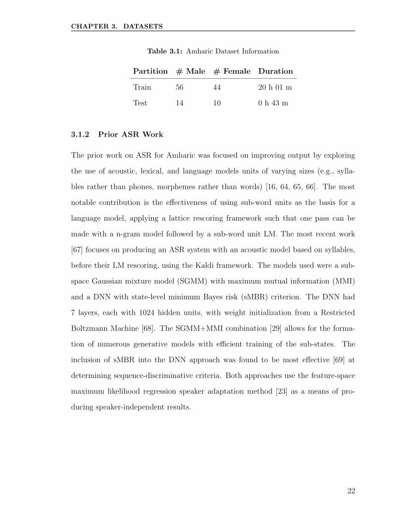
for a total of 10,850 sentences [63]. The duration and speaker information for the
training and test splits are shown in Table 3.1. This dissection of speakers contains
no overlap between the respective training and test sets. The trigram language model
was constructed using the audio transcriptions, as well as other text corpora, resulting
in 120,262 sentences and 2.5 million words [64].
21
CHAPTER 3. DATASETS
Table 3.1: Amharic Dataset Information
Partition # Male # Female Duration
Train 56 44 20 h 01 m
Test 14 10 0 h 43 m
3.1.2 Prior ASR Work
The prior work on ASR for Amharic was focused on improving output by exploring
the use of acoustic, lexical, and language models units of varying sizes (e.g., sylla-
bles rather than phones, morphemes rather than words) [16, 64, 65, 66]. The most
notable contribution is the effectiveness of using sub-word units as the basis for a
language model, applying a lattice rescoring framework such that one pass can be
made with a n-gram model followed by a sub-word unit LM. The most recent work
[67] focuses on producing an ASR system with an acoustic model based on syllables,
before their LM rescoring, using the Kaldi framework. The models used were a sub-
space Gaussian mixture model (SGMM) with maximum mutual information (MMI)
and a DNN with state-level minimum Bayes risk (sMBR) criterion. The DNN had
7 layers, each with 1024 hidden units, with weight initialization from a Restricted
Boltzmann Machine [68]. The SGMM+MMI combination [29] allows for the forma-
tion of numerous generative models with efficient training of the sub-states. The
inclusion of sMBR into the DNN approach was found to be most effective [69] at
determining sequence-discriminative criteria. Both approaches use the feature-space
maximum likelihood regression speaker adaptation method [23] as a means of pro-
ducing speaker-independent results.
22

CHAPTER 3. DATASETS
3.2 Bemba
3.2.1 Language Description
The Bemba (ISO 693-3 bem) language is a member of the Bantu branch of the
Niger-Congo language family spoken by approximately 5 million people, primarily
in Zambia. The Bemba writing system is based on the Latin script, consisting of 23
characters to represent each phoneme in an injective fashion. There are 24 phonemes,
19 consonants and 5 vowels, and are classified into the syllable structure of: vowel,
consonant, nasal, and glide. The corpus [70] was collected outside a closed environ-
ment via read speech from 10 fluent speakers, 6 male and 4 female, for a total of
10,956 sentences. The audio data was purposefully collected in an uncontrolled set-
ting to induce noise and emulate a real-world ASR scenario; each utterance length is
between 1 and 20 words. The duration and speaker information for the training and
test splits are shown in Table 3.2. This subset of speakers contains no overlap between
the respective training and test sets. The trigram language model was constructed
using just the audio transcriptions (123,000, 27,000 unique, words), no additional
improvement was found when using an additional dataset which totaled 5.8 million
(189,000) unique words.
Table 3.2: Bemba Dataset Information
Partition # Male # Female Duration
Train 5 3 14 h 20 m
Test 1 1 1 h 18 m
3.2.2 Prior ASR Work
Previous work on Bemba [70] used the DeepSpeech architecture [55, 71], which re-
quired an initial round of training on a large corpus of English followed by cross-lingual
23

CHAPTER 3. DATASETS
via transfer learning to the small Bemba corpus. The DeepSpeech model was 6 layers:
3 fully connected, followed by a unidirectional LSTM, followed by 2 fully connected
layers. The data was pre-processed to be all lower case and excluded any utterance
longer than 10 seconds long.
3.3 Iban
3.3.1 Language Description
The Iban (ISO 693-3 iba) language is a member of the Malayo-Polynesian branch
of the Austronesian language family spoken by approximately 1.5 million people,
primarily in Borneo. The Iban orthographic system is based on the Latin script,
consisting of 27 characters to represent a 1-to-1 character to phoneme mapping. There
are 30 phonemes, 19 consonants and 11 vowel clusters, and are classified into the
syllable structure of: vowel, consonant, nasal, and glide. The dataset [72] contains no
mention of recording conditions or speaker proficiency, but consists of 23 speakers,
9 male and 14 female, for a total of 3,000 sentences. The duration and speaker
information for the training and test splits are show in Table 3.3. This speaker
partitioning contains no overlap between the training and test sets. The trigram
language model was constructed using the audio transcriptions alongside additional
text scraped from the internet, which totaled 2 million (37,000 unique) words.
Table 3.3: Iban Dataset Information
Partition # Male # Female Duration
Train 7 10 6 h 48 m
Test 2 4 1 h 11 m
24
CHAPTER 3. DATASETS
3.3.2 Prior ASR Work
Previous work on ASR Iban [73, 72] focused on data augmentation and cross-lingual
transfer learning by leveraging similarities between Iban and Malay, a closely related
language with more abundant data. Using Kaldi with feature enhancements similar
to those used for Amharic, Section 3.1.2, the authors trained GMM, SGMM, and
DNN ASR systems, yielding the lowest error rates with the former two architectures.
Their work also notes the effectiveness of speaker adaptation through features like
fMLLR in a GMM model, but ineffectual results within the SGMM and DNN.
3.4 Seneca
3.4.1 Language Description
The Seneca (ISO 693-3 see) language is a member of the Seneca-Cayuga branch of the
Iroquoian language family spoken by around 50 elders and roughly 100 second lan-
guage learners, primarily in western New York, United States, and Ontario, Canada.
The Seneca orthography is based on the Latin script, consisting of 30 characters, which
represent a 1-to-1 grapheme-to-phoneme mapping. The Seneca audio data consists of
spontaneous speech recorded primarily in casual settings over several years from 11
speakers, 7 male and 4 female. The duration and speaker information for the training
and test sets are shown in Table 3.4. This speaker partitioning does contain overlap
between the respective training and test sets due to an in-balance between length of
data per speaker, coupled with few total speakers. The trigram language model was
constructed using a combination of transcripts from the training set and all other
available written texts collected by linguists, missionaries, and anthropologists for a
total of 49,051 (7,625 unique) words.
25
CHAPTER 3. DATASETS
Table 3.4: Seneca Dataset Information
Partition # Male # Female Duration
Train 7 4 9 h 47 m
Test 7 4 01 h 40 m
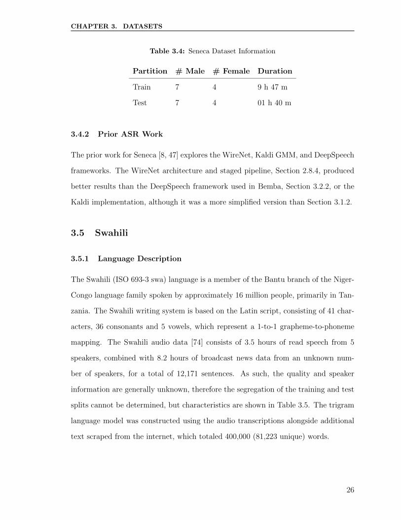
3.4.2 Prior ASR Work
The prior work for Seneca [8, 47] explores the WireNet, Kaldi GMM, and DeepSpeech
frameworks. The WireNet architecture and staged pipeline, Section 2.8.4, produced
better results than the DeepSpeech framework used in Bemba, Section 3.2.2, or the
Kaldi implementation, although it was a more simplified version than Section 3.1.2.
3.5 Swahili
3.5.1 Language Description
The Swahili (ISO 693-3 swa) language is a member of the Bantu branch of the Niger-
Congo language family spoken by approximately 16 million people, primarily in Tan-
zania. The Swahili writing system is based on the Latin script, consisting of 41 char-
acters, 36 consonants and 5 vowels, which represent a 1-to-1 grapheme-to-phoneme
mapping. The Swahili audio data [74] consists of 3.5 hours of read speech from 5
speakers, combined with 8.2 hours of broadcast news data from an unknown num-
ber of speakers, for a total of 12,171 sentences. As such, the quality and speaker
information are generally unknown, therefore the segregation of the training and test
splits cannot be determined, but characteristics are shown in Table 3.5. The trigram
language model was constructed using the audio transcriptions alongside additional
text scraped from the internet, which totaled 400,000 (81,223 unique) words.
26
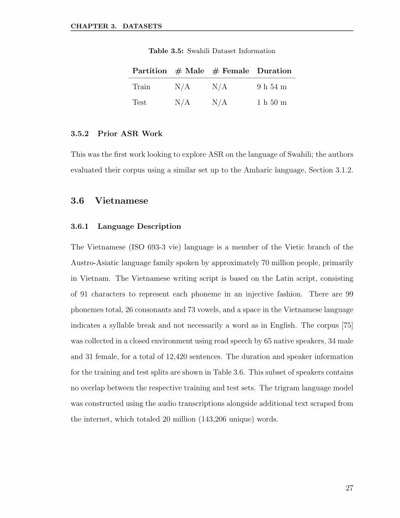
CHAPTER 3. DATASETS
Table 3.5: Swahili Dataset Information
Partition # Male # Female Duration
Train N/A N/A 9 h 54 m
Test N/A N/A 1 h 50 m
3.5.2 Prior ASR Work
This was the first work looking to explore ASR on the language of Swahili; the authors
evaluated their corpus using a similar set up to the Amharic language, Section 3.1.2.
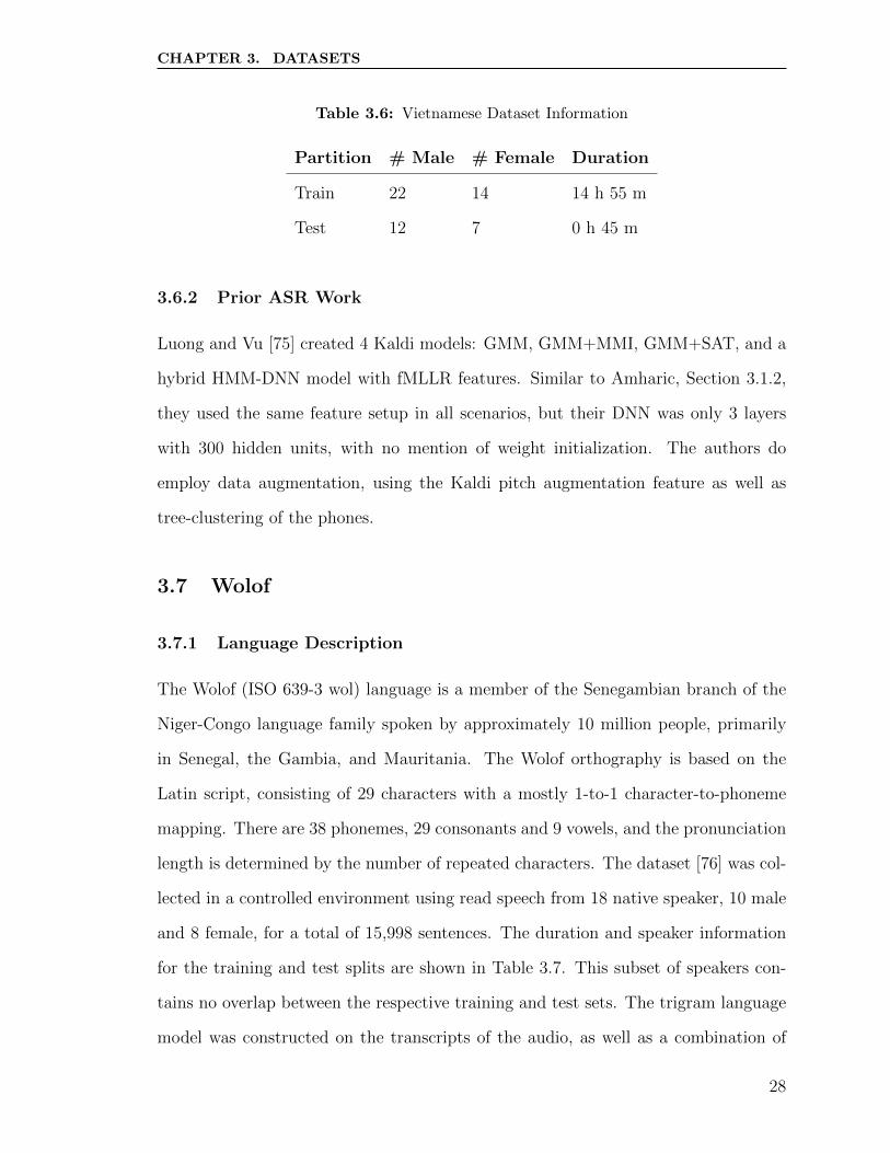
3.6 Vietnamese
3.6.1 Language Description
The Vietnamese (ISO 693-3 vie) language is a member of the Vietic branch of the
Austro-Asiatic language family spoken by approximately 70 million people, primarily
in Vietnam. The Vietnamese writing script is based on the Latin script, consisting
of 91 characters to represent each phoneme in an injective fashion. There are 99
phonemes total, 26 consonants and 73 vowels, and a space in the Vietnamese language
indicates a syllable break and not necessarily a word as in English. The corpus [75]
was collected in a closed environment using read speech by 65 native speakers, 34 male
and 31 female, for a total of 12,420 sentences. The duration and speaker information
for the training and test splits are shown in Table 3.6. This subset of speakers contains
no overlap between the respective training and test sets. The trigram language model
was constructed using the audio transcriptions alongside additional text scraped from
the internet, which totaled 20 million (143,206 unique) words.
27
CHAPTER 3. DATASETS
Table 3.6: Vietnamese Dataset Information
Partition # Male # Female Duration
Train 22 14 14 h 55 m
Test 12 7 0 h 45 m
3.6.2 Prior ASR Work
Luong and Vu [75] created 4 Kaldi models: GMM, GMM+MMI, GMM+SAT, and a
hybrid HMM-DNN model with fMLLR features. Similar to Amharic, Section 3.1.2,
they used the same feature setup in all scenarios, but their DNN was only 3 layers
with 300 hidden units, with no mention of weight initialization. The authors do
employ data augmentation, using the Kaldi pitch augmentation feature as well as
tree-clustering of the phones.
3.7 Wolof
3.7.1 Language Description
The Wolof (ISO 639-3 wol) language is a member of the Senegambian branch of the
Niger-Congo language family spoken by approximately 10 million people, primarily
in Senegal, the Gambia, and Mauritania. The Wolof orthography is based on the
Latin script, consisting of 29 characters with a mostly 1-to-1 character-to-phoneme
mapping. There are 38 phonemes, 29 consonants and 9 vowels, and the pronunciation
length is determined by the number of repeated characters. The dataset [76] was col-
lected in a controlled environment using read speech from 18 native speaker, 10 male
and 8 female, for a total of 15,998 sentences. The duration and speaker information
for the training and test splits are shown in Table 3.7. This subset of speakers con-
tains no overlap between the respective training and test sets. The trigram language
model was constructed on the transcripts of the audio, as well as a combination of
28

CHAPTER 3. DATASETS
physical books and data scraped from the internet, for a total of 601,609 (29,148
unique) words.
Table 3.7: Wolof Dataset Information
Partition # Male # Female Duration
Train 8 6 16 h 49 m
Test 1 1 0 h 55 m
3.7.2 Prior ASR Work
This was the first work looking to explore ASR on the language of Wolof; the au-
thors evaluated their corpus using a similar set up to the Amharic language, Section
3.1.2. In a subsequent paper, the authors found that modeling vowel length contrasts
improved word error rate [77].
29

Chapter 4
Methodology
As there are numerous corpora spanning varying morphologies and ASR implementa-
tions, it will be beneficial to standardize the results across these languages to deter-
mine what combination of input feature, acoustic, and language model can produce
the best result or if the combination differs per language structure.
4.1 Language Comparison
4.1.1 Average Utterance Length
As described prior, the ability of a DNN to aptly model a speech signal is dependent
on the width of the layers, but wider layers require more time to reach convergence.
Therefore, if we can simply reduce the length of the audio signal, there is less need for
such wide of layers. Each language was measured for mean utterance length (MUL),
with the intention to create data subsets with a MUL less than 5, 10, or 15 seconds to
determine the correlation between MUL and WER, as studies have indicated natural
language understanding can occur in as few as 6 words [78].
4.1.2 Quality Measures
Another potential insight into the language differences is recording quality; some
languages are purposefully recorded in a conversational tone with extraneous noise
30

CHAPTER 4. METHODOLOGY
unfiltered, others with studio quality sound equipment, while others still use radio or
television broadcasts. Each recording condition will contain some measure of back-
ground noise, and although preliminary research indicates that noise can be naturally
removed [48], human speech comprehension is based on the recognition of both voiced
and unvoiced pieces. Two measures of quality were conducted on the languages: Na-
tional Institute of Standards and Technology’s (NIST) speech Signal to Noise Ratio
(SNR) and Waveform Amplitude Distribution Analysis (WADA) SNR. General SNR
is defined through Equation 4.1, where the signal x(t) = s(t) + n(t), these two tools
work to evaluate the SNR of an entire audio signal.
SNRdB(x) = 10 log10
Power(s)
Power(n)(4.1)
NIST’s SNR measurement tool uses a sequential GMM to model the speech data,
before being evaluated by the Kolmogrov-Smirnov statistic for goodness of fit. If
a reasonably good fit is achieved, the mixtures are estimated using the standard
Expectation Maximization (EM) steps, producing a quality estimate.
WADA’s SNR algorithm examines the gamma distribution of the amplitude, not-
ing that the probability density function of said gamma distribution can be shaped
to estimate SNR [3]. Through an experiment with heavy noise dilation on a news
database, Kim and Stern [3] found that the WADA algorithm more closely mimicked
the expected speech quality, Figure 4.1, with a separate group confirming [79] against
a different corpus.
31

CHAPTER 4. METHODOLOGY
Figure 4.1: Comparison of the WADA SNR algorithm and the average estimated NISTSNR against an artificially corrupted database. [3]
4.2 Kaldi
There were several Kaldi implementations presented by the prior ASR work [67, 73,
72, 8, 47, 75, 76], but we focused on the well documented version in Gauthier et al.
[76]. The models were cascaded together, beginning with 13 MFCCs, their delta delta
coefficients, transformed via LDA, MLLT, and fMLLR. These features were passed
into triphone GMM models with 3,401 context-dependent states and 40k Gaussians.
The SGMM was trained and rescored a total of 8 times, broadening the GMM sub-
32
CHAPTER 4. METHODOLOGY
space construction, before final rescoring from MBR and FMMI [80]. The DNN
was built on 6 hidden layers of 1024 units and trained using 11 consecutive frames
and state-level minimum Bayes risk (sMBR) criterion, with weight initialization from
RBMs, before final finetuning using Stochastic Gradient Descent.
We also investigated Kaldi with data augmentation, similar to Luong et al. [75],
in order to explore whether addition data will improve ASR accuracy within this
framework.
4.3 WireNet
The WireNet architecture [8] was capable of producing state-of-the-art results on
the low-resource language of Seneca, we investigate whether these improvements will
extend to other available ASR corpora with varying linguistic properties and corpus
features, such as speaker pool size, speaker diversity, and SNR.
4.3.1 Transfer Learning
The first step in the WireNet pipeline is transfer learning from a high resource lan-
guage, typically English. Transfer learning has been seen as critical to a low-resource
language ASR system [34, 81], but produces a large overhead whenever the internal
architecture changes, requiring re-learning for this new structure.
4.3.2 Data Augmentation
The second stage in the aforementioned pipeline is inclusion of additional data in the
training set as a means of artificially boosting the amount of available audio to be
able to emulate a higher resourced language.
33

CHAPTER 4. METHODOLOGY
4.3.2.1 Speech Synthesis
In a low-resource scenario, not only is the number of utterances limited, but also
the speakers themselves. These corpora have taken great care to isolate the training
and test set speakers, barring Seneca, limiting the already low amount. Textual
data, however, is often prevalent for these languages; therefore, we might be able to
synthesize a speaker from the training set from their audio samples and reapply their
voice to a new textual utterance. This will improve not only the dataset duration,
but also quality as the vocabulary will increase.
4.3.2.2 Pitch/Time Shifting
More simple methods of data augmentation keep the same linguistic content, altering
the phonetic and acoustic properties. Here we base the augmentation methods on
those from the Jimerson et al. [47, 8], adjusting the fundamental frequency and
speaking rate. Pitch augmentation was performed by varying the frequency by a
randomly chosen octave ranging from 0.10 to 0.25, with a step size of 0.05. Speed
shifting was performed by re-sampling the audio at a different, randomly chosen
frequency ranging from 0.75 to 1.25, with a step size of 0.05. Each utterance in the
training set was distorted randomly 10 times and added alongside the original data,
totaling an average increase of 1000%.
4.3.3 Architecture Exploration
The original architecture from WireNet, Figure 2.4, depicts 5 bottleneck block layers,
where each bottleneck contained 9 incrementally varying, odd width kernel sizes. The
author mentions that these filter widths are chosen to pick up both short- and long-
term dependencies [8] but contains no mention of how these numbers were selected.
Additionally, the number of filters per convolutional layer could also be an area of
improvement, as inverted linear bottlenecks [82] have shown to produce effective con-
34
CHAPTER 4. METHODOLOGY
vergence. Therefore, we aim to determine the optimal width, depth, and bottleneck
size for these various languages in a hope to understand the author’s numerical selec-
tions. Additionally, we attempt to arrange these bottleneck blocks in various schema
from other state-of-the-art producing architectures such as U-Net [4], Selective Kernel
Networks [83], or Time Delay Neural Network [84].
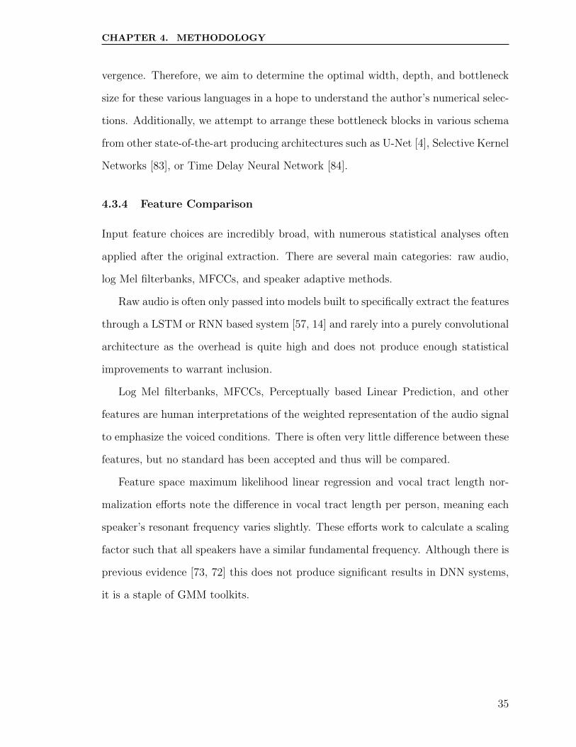
4.3.4 Feature Comparison
Input feature choices are incredibly broad, with numerous statistical analyses often
applied after the original extraction. There are several main categories: raw audio,
log Mel filterbanks, MFCCs, and speaker adaptive methods.
Raw audio is often only passed into models built to specifically extract the features
through a LSTM or RNN based system [57, 14] and rarely into a purely convolutional
architecture as the overhead is quite high and does not produce enough statistical
improvements to warrant inclusion.
Log Mel filterbanks, MFCCs, Perceptually based Linear Prediction, and other
features are human interpretations of the weighted representation of the audio signal
to emphasize the voiced conditions. There is often very little difference between these
features, but no standard has been accepted and thus will be compared.
Feature space maximum likelihood linear regression and vocal tract length nor-
malization efforts note the difference in vocal tract length per person, meaning each
speaker’s resonant frequency varies slightly. These efforts work to calculate a scaling
factor such that all speakers have a similar fundamental frequency. Although there is
previous evidence [73, 72] this does not produce significant results in DNN systems,
it is a staple of GMM toolkits.
35

CHAPTER 4. METHODOLOGY
4.4 Speaker Re-partitioning
In addition to the toolkit specific adjustments, we also want to examine the impor-
tance of the dataset construction. Specifically noted in the corpora statistics is that
the training and test sets contain disjoint speakers. However, in Seneca, as in most
endangered languages, there are simply not enough speakers to create speaker-disjoint
training and testing sets. We tested both purposeful withholding of speakers, along-
side purely random construction to investigate the effectiveness of speaker overlap
between the two sets. An important distinction is that the audio transcriptions will
not be duplicated in any manner, the utterances maintain their uniqueness such that
the systems will not be overfit to one sentence.
4.5 Language Model Exploration
Alongside the acoustic model exploration, the language model rescoring is essential
towards quality results from the system. On top of the standard n-gram models, we
aim to investigate a LSTM LM [43, 54] capable of producing state-of-the-art results
across numerous systems [85, 14].
36

Chapter 5
Results
5.1 Kaldi Results
5.1.1 Overall
The normalization of the results across these various languages begins with the stan-
dardized experiments with the Kaldi setup, these results are shown in Table 5.1. The
top two architectures are displayed, the SGMM and DNN variants, with the best
WER taken from each model’s most successful iteration.
Table 5.1: Overall Kaldi results for the two best architectures across all languages.
LanguageModel Relative Reduction in WER
SGMM DNN
Amharic 8.4 7.5 10.71
Bemba 58.4 53.4 8.56
Iban 16.4 15.1 7.93
Seneca 33.9 30.6 9.73
Swahili 27.3 26.5 2.93
Vietnamese 9.7 9.5 2.06
Wolof 25.1 24.9 0.80
Notably, for every model the DNN performed best, with often improvements up to
37
CHAPTER 5. RESULTS
8% over the SGMM. Additionally, the results for the Bemba and Iban are the lowest
word error rates uncovered thus far: 54.78 [70] vs. 53.4 and 18.1 [72] vs. 15.1, with
the Vietnamese matching the state-of-the-art result to the tenth decimal place, 9.48
[75] vs 9.53. Of note, this was the best non-WireNet Seneca result produced, 42.1 [8]
vs. 30.6. For the other languages, this was the recipe used by the authors [76] and
thus no improvements found.
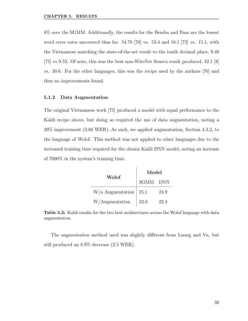
5.1.2 Data Augmentation
The original Vietnamese work [75] produced a model with equal performance to the
Kaldi recipe above, but doing so required the use of data augmentation, noting a
29% improvement (3.86 WER). As such, we applied augmentation, Section 4.3.2, to
the language of Wolof. This method was not applied to other languages due to the
increased training time required for the chosen Kaldi DNN model, noting an increase
of 7000% in the system’s training time.
WolofModel
SGMM DNN
W/o Augmentation 25.1 24.9
W/Augmentation 23.0 22.4
Table 5.2: Kaldi results for the two best architectures across the Wolof language with dataaugmentation.
The augmentation method used was slightly different from Luong and Vu, but
still produced an 8.9% decrease (2.5 WER).
38
CHAPTER 5. RESULTS
5.2 WireNet
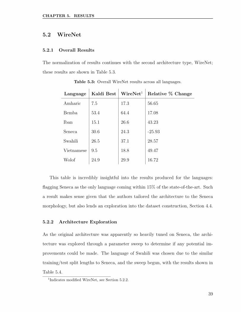
5.2.1 Overall Results
The normalization of results continues with the second architecture type, WireNet;
these results are shown in Table 5.3.
Table 5.3: Overall WireNet results across all languages.
Language Kaldi Best WireNet1 Relative % Change
Amharic 7.5 17.3 56.65
Bemba 53.4 64.4 17.08
Iban 15.1 26.6 43.23
Seneca 30.6 24.3 -25.93
Swahili 26.5 37.1 28.57
Vietnamese 9.5 18.8 49.47
Wolof 24.9 29.9 16.72
This table is incredibly insightful into the results produced for the languages:
flagging Seneca as the only language coming within 15% of the state-of-the-art. Such
a result makes sense given that the authors tailored the architecture to the Seneca
morphology, but also lends an exploration into the dataset construction, Section 4.4.
5.2.2 Architecture Exploration
As the original architecture was apparently so heavily tuned on Seneca, the archi-
tecture was explored through a parameter sweep to determine if any potential im-
provements could be made. The language of Swahili was chosen due to the similar
training/test split lengths to Seneca, and the sweep begun, with the results shown in
Table 5.4.
1Indicates modified WireNet, see Section 5.2.2.
39

CHAPTER 5. RESULTS
Table 5.4: WireNet architecture exploration for Swahili, varying the width and depth ofthe system.
Depth Width WER CER
5 9 42.384 19.281
6 9 46.707 20.269
7 9 51.277 22.037
8 9 56.271 28.412
4 9 42.809 18.032
3 9 43.546 18.916
4 10 42.263 17.958
4 8 45.970 20.286
4 11 40.908 17.427
4 15 39.663 17.223
4 21 37.136 16.47
3 21 42.418 19.362
Analyzing the table indicates that Swahili, an agglutinative, morphologically rich
language, performed best with a shorter, wider network; this can apply to the sim-
ilarly morphologically complex African languages of Amharic and Wolof. Through
experimental results, this modified WireNet of a depth of 4 and width of 21 pro-
duced marginally (1-3%) better results across the board no matter which language
was tested.
Additionally, the bottleneck size was investigated, as an inverted linear bottleneck
has been shown to improve convergence time [82], with a trade-off of memory usage,
shown in Figure 5.1.
40

CHAPTER 5. RESULTS
Figure 5.1: CER vs. training epochs of the Swahili language at specific bottleneck depths.
This exploration shows that there is a point at which the error rate converges more
quickly, around a bottleneck depth of 256, and after that the increase can actually be
harmful. Note that this did not improve the WER of the system, only the convergence
time; it did however increase training time as the GPU memory required for these
larger widths reduced the potential batch size. During this exploration it became
evident that the transfer learning step introduced by Wav2Vec [57] and utilized by
WireNet [8] is not helpful towards the speed of convergence; the majority decreases
during the augmentation step; explored further in 5.2.3.
The architecture was additionally structured in a similar manner to U-net [4],
Figure 5.2.
41

CHAPTER 5. RESULTS
Figure 5.2: U-Net architecture where the convolutional size increases to a maximum of1024, before reducing back to the input size. [4]
To reproduce the U-Net state-of-the-art models in a different domain, the bottle-
neck blocks were cascaded in a similar style to Figure 5.2, with evaluation performed
on the language of Swahili, shown in Table 5.5.
Table 5.5: WireNet results for the Swahili language with U-Net styled architecture.
Language WER
Swahili 67.83
Such an architecture was unsuitable for this application, as the model parameters
were too large, with not enough training data or time available for convergence to
occur.
42

CHAPTER 5. RESULTS
5.2.3 Transfer Learning
Transfer learning is often seen as critical to the success of a low-resource language
ASR system [34, 81, 14, 15, 72], but when performing an architecture exploration such
as above, it is incredibly time consuming to re-train the model on this high-resource
dataset to where suitable results have been attained. Therefore, we investigated the
efficacy of said step.
Figure 5.3: CER vs. training epochs through the stages of training the Swahili languagewith transfer learning.
During the transfer learning stage from a high-level language, the CER begins
at a less than 100% because of this initialization; however, due to the dissimilarity
between languages, the first few epochs are seen re-learning these weights. As such,
the CER increases initially, before decreasing once these prior weights are overwritten.
Essentially this step just trains directly on the clean, unaugmented data itself for an
extra stage. Beginning training on the augmented data, Figure 5.4, removes this
superfluous step and achieves the same end word error rate.
43

CHAPTER 5. RESULTS
Figure 5.4: CER vs. training epochs through the stages of training the Swahili languagewithout transfer learning.
This breakthrough also unveiled another: the finetune stage was stagnating once
the model was trained to convergence on the augmented data. Applying a learning
rate scheduler to the CTC loss, potentially allowing for the finetune stage to better
suit its name, but in actuality indicating a more suitable early stopping point.
5.2.4 Feature Comparison
The ability to model the different linguistic properties of languages is impacted by
the input features used, shown in Table 5.6.
44

CHAPTER 5. RESULTS
Table 5.6: Feature Comparison of Languages
Language Feature WER CER
Seneca MFCC 29.9 17.5
Seneca FBANK 24.3 13
Swahili MFCC 51.277 22.037
Swahili FBANK 56.271 28.412
Amharic MFCC 18.233 9.263
Amharic FBANK 17.346 8.962
Vietnamese MFCC 18.829 11.495
Vietnamese FBANK 18.130 9.621
As one goal is to standardize the model parameters, and input features can take
many forms, results such as Table 5.6 indicate that the filterbank features themselves,
without the additional discrete cosine transform, perform better. This holds for 5 of
the 7 languages tested, although arguments may be made for quality and extraneous
factors being the reason for better WireNet performance in Swahili and Wolof as
opposed to the input feature.
Additionally, the Kaldi introduced feature of fMLLR was used on the Wolof
dataset, with the effects of speaker normalization evident on the architecture per-
formance, shown in Table 5.7.
Table 5.7: Feature Comparison of Wolof
Feature WER CER
MFCC 29.882 11.149
FBANK 30.331 11.792
fMLLR 35.922 13.689
Similar to the work on Iban [73, 72], the application of speaker normalization did
45

CHAPTER 5. RESULTS
not improve the system performance, heavily in the opposite direction in fact. As
other methods are attempted to introduce speaker normalization, Section 4.4, remove
this feature from the Kaldi schema may prove fruitful.
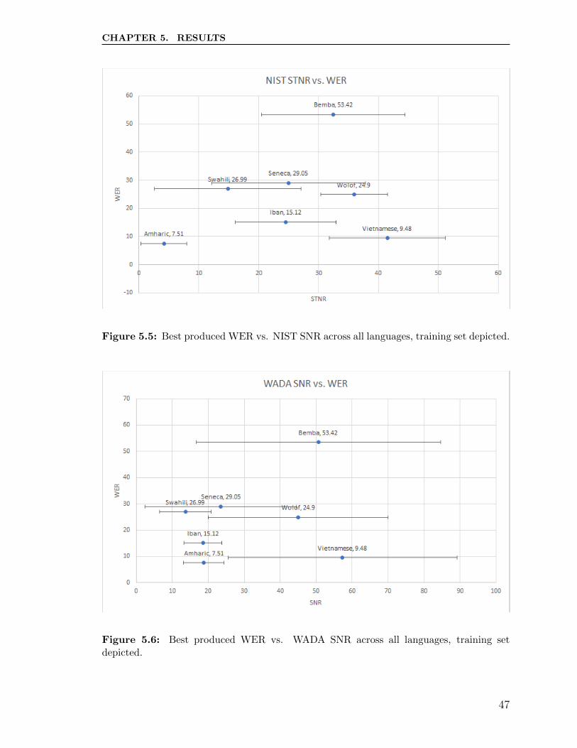
5.3 Language Comparison
To attempt to clarify the reasoning behind design choices such as input feature repre-
sentation or results such as word error rate, the quality of the datasets was evaluated
using the standard signal to noise ratio calculators, displayed in Table 5.8 alongside
visually in Figures 5.5 and 5.6.
Table 5.8: SNR overview per language.
LanguageNIST SNR WADA SNR
Train Test Train Test
Amharic 4.19 ± 3.83 18.80 ± 5.69 4.85 ± 3.37 17.978 ± 7.24
Bemba 32.46 ± 12.01 50.65 ± 33.92 27.47 ± 9.75 36.27 ± 22.52
Iban 24.51 ± 8.43 18.54 ± 5.28 22.65 ± 8.79 17.23 ± 4.32
Seneca 24.96 ± 12.85 23.51 ± 21.07 25.19 ± 13.14 25.72 ± 24.02
Swahili 14.84 ± 12.23 13.66 ± 7.13 16.77 ± 12.22 15.68 ± 5.92
Vietnamese 41.48 ± 9.70 57.32 ± 31.86 37.68 ± 11.05 55.62 ± 36.37
Wolof 35.92 ± 5.59 45.03 ± 34.99 35.39 ± 3.77 38.08 ± 14.59
We see that Bemba, Iban, and Wolof have comparable SNR under both methods
of calculation, while the SNR for Amharic is substantially lower than the others under
the NIST method but comparable to Iban under the WADA method. We also observe
much less variation in SNR for Iban and Amharic than for the other languages, while
the Seneca, Wolof, and Vietnamese contain a great measure of variability, specifically
in the test sets.
46
CHAPTER 5. RESULTS
Figure 5.5: Best produced WER vs. NIST SNR across all languages, training set depicted.
Figure 5.6: Best produced WER vs. WADA SNR across all languages, training setdepicted.
47
CHAPTER 5. RESULTS
There does not appear to be an indication between dataset quality and word error
rate; as Li et al. hypothesized [48], the DNN naturally normalized the heterogeneous
data.
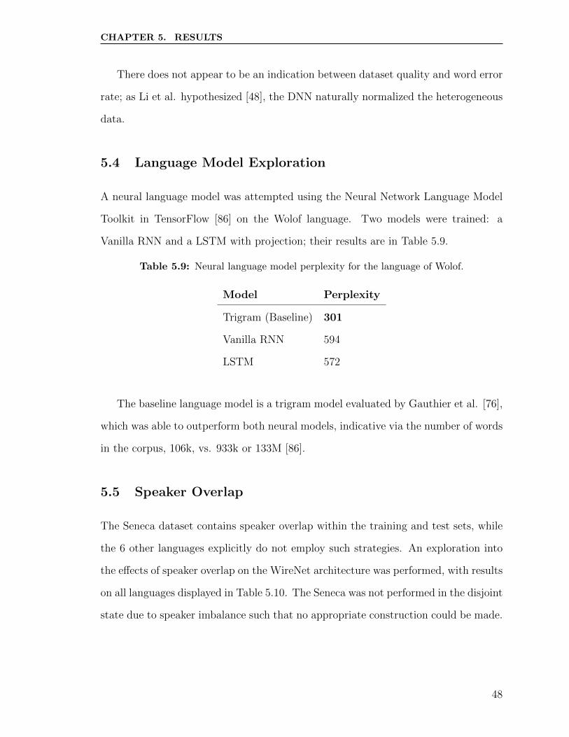
5.4 Language Model Exploration
A neural language model was attempted using the Neural Network Language Model
Toolkit in TensorFlow [86] on the Wolof language. Two models were trained: a
Vanilla RNN and a LSTM with projection; their results are in Table 5.9.
Table 5.9: Neural language model perplexity for the language of Wolof.
Model Perplexity
Trigram (Baseline) 301
Vanilla RNN 594
LSTM 572
The baseline language model is a trigram model evaluated by Gauthier et al. [76],
which was able to outperform both neural models, indicative via the number of words
in the corpus, 106k, vs. 933k or 133M [86].
5.5 Speaker Overlap
The Seneca dataset contains speaker overlap within the training and test sets, while
the 6 other languages explicitly do not employ such strategies. An exploration into
the effects of speaker overlap on the WireNet architecture was performed, with results
on all languages displayed in Table 5.10. The Seneca was not performed in the disjoint
state due to speaker imbalance such that no appropriate construction could be made.
48
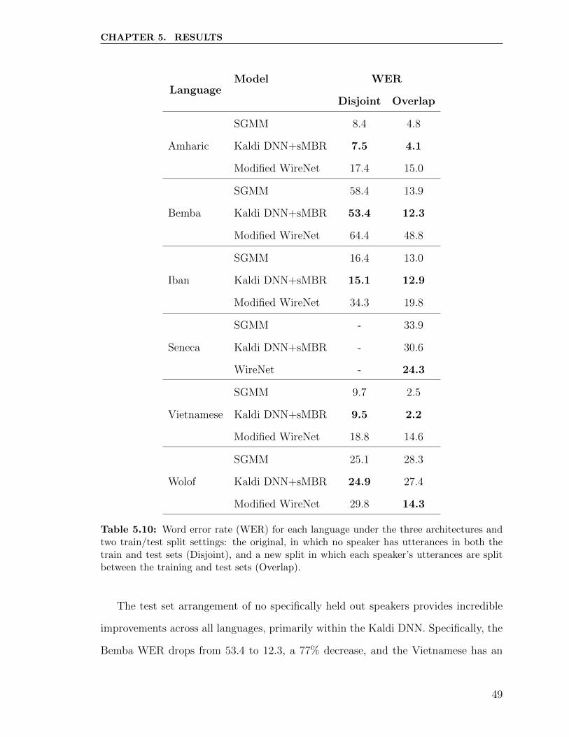
CHAPTER 5. RESULTS
LanguageModel WER
Disjoint Overlap
Amharic
SGMM 8.4 4.8
Kaldi DNN+sMBR 7.5 4.1
Modified WireNet 17.4 15.0
Bemba
SGMM 58.4 13.9
Kaldi DNN+sMBR 53.4 12.3
Modified WireNet 64.4 48.8
Iban
SGMM 16.4 13.0
Kaldi DNN+sMBR 15.1 12.9
Modified WireNet 34.3 19.8
Seneca
SGMM - 33.9
Kaldi DNN+sMBR - 30.6
WireNet - 24.3
Vietnamese
SGMM 9.7 2.5
Kaldi DNN+sMBR 9.5 2.2
Modified WireNet 18.8 14.6
Wolof
SGMM 25.1 28.3
Kaldi DNN+sMBR 24.9 27.4
Modified WireNet 29.8 14.3
Table 5.10: Word error rate (WER) for each language under the three architectures andtwo train/test split settings: the original, in which no speaker has utterances in both thetrain and test sets (Disjoint), and a new split in which each speaker’s utterances are splitbetween the training and test sets (Overlap).
The test set arrangement of no specifically held out speakers provides incredible
improvements across all languages, primarily within the Kaldi DNN. Specifically, the
Bemba WER drops from 53.4 to 12.3, a 77% decrease, and the Vietnamese has an
49

CHAPTER 5. RESULTS
almost unbelievable 2.2% WER, although their word boundaries were more syllabic
[75], this is still impressive. The two outliers are the languages of Seneca and Wolof,
where the WireNet models performed strikingly better than Kaldi.
Given the vast reductions in WER using this method, we investigated at which
point the test set construction could be hindered by containing too few of the speakers.
With this in mind, we performed specific speaker holdouts from those whose total
combined utterance lengths were less than the test set time, such that the test set
may contain more than one speaker. The results for the Bemba, Seneca, and Wolof
languages are present in Tables 5.11, 5.12, 5.13 and Figures 5.7, 5.8, 5.9, respectively.
Speaker Withheld Duration (s) % of Total % of Test WER
1 24670.82 43.84 - -
3 14854.03 26.40 - -
5 7310.515 12.99 - -
4 3326.315 5.91 71.08 8.6
6 1951.42 3.47 41.70 29.22
7 711.5254 1.26 15.20 13.43
8 189.3953 0.34 4.05 14.1
9 349.9815 0.62 7.48 15.01
10 218.1657 0.39 4.66 11.82
12 2686.953 4.78 57.41 33.97
None - - 0 12.32
6, 12 (default) 4638.373 - 100.00 53.42
Even - - - 21.98
Table 5.11: Determining the impact of holding out each speaker for the Bemba language.
50
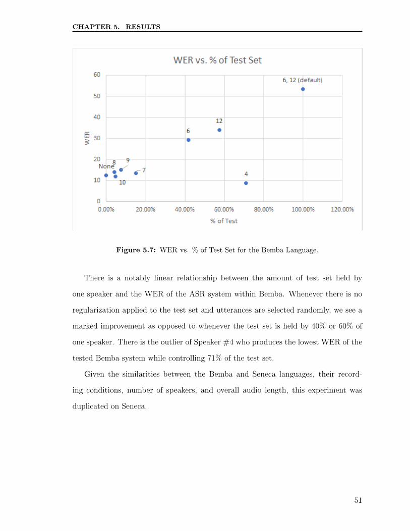
CHAPTER 5. RESULTS
Figure 5.7: WER vs. % of Test Set for the Bemba Language.
There is a notably linear relationship between the amount of test set held by
one speaker and the WER of the ASR system within Bemba. Whenever there is no
regularization applied to the test set and utterances are selected randomly, we see a
marked improvement as opposed to whenever the test set is held by 40% or 60% of
one speaker. There is the outlier of Speaker #4 who produces the lowest WER of the
tested Bemba system while controlling 71% of the test set.
Given the similarities between the Bemba and Seneca languages, their record-
ing conditions, number of speakers, and overall audio length, this experiment was
duplicated on Seneca.
51
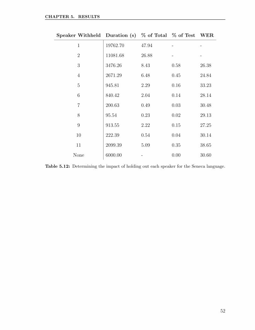
CHAPTER 5. RESULTS
Speaker Withheld Duration (s) % of Total % of Test WER
1 19762.70 47.94 - -
2 11081.68 26.88 - -
3 3476.26 8.43 0.58 26.38
4 2671.29 6.48 0.45 24.84
5 945.81 2.29 0.16 33.23
6 840.42 2.04 0.14 28.14
7 200.63 0.49 0.03 30.48
8 95.54 0.23 0.02 29.13
9 913.55 2.22 0.15 27.25
10 222.39 0.54 0.04 30.14
11 2099.39 5.09 0.35 38.65
None 6000.00 - 0.00 30.60
Table 5.12: Determining the impact of holding out each speaker for the Seneca language.
52

CHAPTER 5. RESULTS
Figure 5.8: WER vs. % of Test Set for the Seneca Language.
Such a linear relationship is also seen in the Seneca language; however, this is less
of a slope and more of a constant line. There is once again an outlier of Speaker #4
who produces the lowest WER of the tested Seneca system while controlling 44.5%
of the test set. Additionally, this result from Speaker #4 comes incredibly close to
the WireNet state-of-the-art result of 24.3 WER. There is no indication that holding
out specific speakers has a beneficial effect on the overall WER of the system, but for
assurance we tested again on the similar language of Wolof.
53

CHAPTER 5. RESULTS
Speaker Withheld Duration (s) % of Total % of Test WER
1 4327.68 6.77 86.55 29.91
2 4226.22 6.61 84.52 25.34
4 4788.99 7.49 95.78 36.34
5 906.99 1.42 18.14 27.27
7 4129.59 6.46 82.59 28.87
8 4274.32 6.69 85.49 24.81
9 4903.53 7.67 98.07 38.02
10 2412.76 3.78 48.26 26.37
11 4697.13 7.35 93.94 31.17
12 4569.61 7.15 91.39 28.29
13 4803.69 7.52 96.07 27.55
14 4024.33 6.30 80.49 31.51
15 4237.14 6.63 84.74 24.15
16 3894.48 6.09 77.89 33.80
17 3796.23 5.94 75.92 31.68
18 3919.57 6.13 78.39 28.83
5, 10 (Default) 3319.75 5.19 100.00 24.90
None 3350.00 5.24 0.00 27.40
Table 5.13: Determining the impact of holding out each speaker for the Wolof language.
54

CHAPTER 5. RESULTS
Figure 5.9: WER vs. % of Test Set for the Wolof Language.
The Wolof language can clearly indicate, similar to the Seneca language, that
there is a WER threshold reached by the system, and although there are variations
according to the percentage of the test set, no improvements seen. This raises the
question of why the Bemba language performs so excellent with the overlap, leading
us to the comparison of the SNR, 5.6. In a low-resource scenario with a high SNR
due to poor recording conditions, overlapping the speakers in the training and test set
can provide noticeable improvements in the Kaldi framework. In the WireNet archi-
tecture, this speaker enhancement trait allows for appreciable improvements across
the board, yet they fall short of the state-of-the-art, but it is an effective tool to
potentially improve accuracy greatly.
55

Chapter 6
Conclusions
6.1 Conclusions
The goal of this thesis is to develop a one-stop shop knowledge base of properly apply-
ing the state-of-the-art toolkits to low-resource languages. We explored architecture
configurations for a cascaded hidden Markov model-based solution using statistical
and deep learning methodologies. In addition, we propose improvements to a novel,
fully convolutional neural network model that allows for the skipping of the time-
consuming transfer learning stage, as well as general architecture adjustments which
better suit an array of various morphological languages. We evaluated the effec-
tiveness of various input features, acoustic, and language models to determine the
efficacy of each component’s various derivatives. The results show that the log Mel
filterbanks are generally most effective at the convolutional level, while speaker adap-
tive methods perform better in a SGMM. Additionally, the combination of a simple
DNN coupled with statistical methodology like state-level minimum Bayes risk allows
for state-of-the-art calculation across the board.
We also note the use of data re-partitioning where utterances are withheld for a
test set as opposed to speakers themselves. This allowed for the acoustic models to
vastly improve their ASR capabilities, with some languages noting a 77% improve-
ment in word error rate. We note that six of these seven languages, while having
56

CHAPTER 6. CONCLUSIONS
few acoustic training resources, are widely spoken and have established written tra-
ditions adequate to support the training of large language models and the collection
of additional data. Any ASR system built for these languages should be robust to
speaker variation. A substantial majority of the world’s 7000 languages, however,
are endangered and in need of documentation and preservation, much like Seneca.
Architectures designed specifically to be speaker independent may not be the best
option for the documentation of languages with very few speakers.
6.2 Future Work
• Continued experimentation with these architecture constructions and others,
e.g., Kaldi’s Time Delay Neural Network, for available small corpora.
• Additional work with data augmentation as there are noted improvements in
acoustic modeling systems.
• Further investigation into speaker overlap in the train/test set while maintaining
utterance uniqueness, including technologies such as speech synthesis.
• Multi-lingual sequence-to-sequence models have shown to be a promising up-
and-coming technology and may improve the low-resource field.
57
Bibliography
[1] K. Selvan and K. K. Anish Babu, “Text independent automatic speaker recog-nition system in malayalam,” in 2013 International Conference on AdvancedComputing and Communication Systems, 2013, pp. 1–4.
[2] D. S. Park, W. Chan, Y. Zhang, C.-C. Chiu, B. Zoph, E. D. Cubuk,and Q. V. Le, “Specaugment: A simple data augmentation method forautomatic speech recognition,” Interspeech 2019, Sep 2019. [Online]. Available:http://dx.doi.org/10.21437/Interspeech.2019-2680
[3] C. Kim and R. Stern, “Robust signal-to-noise ratio estimation based on waveformamplitude distribution analysis,” 01 2008, pp. 2598–2601.
[4] O. Ronneberger, P. Fischer, and T. Brox, “U-net: Convolutional networks forbiomedical image segmentation,” CoRR, vol. abs/1505.04597, 2015. [Online].Available: http://arxiv.org/abs/1505.04597
[5] S. Ruan, J. O. Wobbrock, K. Liou, A. Ng, and J. A. Landay, “Comparing speechand keyboard text entry for short messages in two languages on touchscreenphones,” Proc. ACM Interact. Mob. Wearable Ubiquitous Technol., vol. 1, no. 4,Jan. 2018. [Online]. Available: https://doi.org/10.1145/3161187
[6] C.-C. Chiu, T. N. Sainath, Y. Wu, R. Prabhavalkar, P. Nguyen, Z. Chen, A. Kan-nan, R. J. Weiss, K. Rao, E. Gonina, N. Jaitly, B. Li, J. Chorowski, and M. Bac-chiani, “State-of-the-art speech recognition with sequence-to-sequence models,”2018.
[7] “How many languages are there in the world?” Feb 2020. [Online]. Available:https://www.ethnologue.com/guides/how-many-languages
[8] B. Thai, “Deepfake detection and low-resource language speech recognition usingdeep learning,” Thesis, Rochester Institute of Technology, 2019.
[9] R. Collobert, C. Puhrsch, and G. Synnaeve, “Wav2letter: an end-to-end convnet-based speech recognition system,” 2016.
[10] H. Sailor, A. Patil, and H. Patil, “Advances in Low Resource ASR: A DeepLearning Perspective,” in Proc. The 6th Intl. Workshop on Spoken LanguageTechnologies for Under-Resourced Languages, 2018, pp. 15–19. [Online].Available: http://dx.doi.org/10.21437/SLTU.2018-4
[11] Y. Hoshen, R. J. Weiss, and K. W. Wilson, “Speech acoustic modeling from rawmultichannel waveforms,” in 2015 IEEE International Conference on Acoustics,Speech and Signal Processing (ICASSP), 2015, pp. 4624–4628.
58
BIBLIOGRAPHY
[12] M. Ravanelli and Y. Bengio, “Speech and speaker recognition from raw waveformwith sincnet,” 2019.
[13] N. Zeghidour, N. Usunier, G. Synnaeve, R. Collobert, and E. Dupoux, “End-to-end speech recognition from the raw waveform,” 2018.
[14] A. Baevski, H. Zhou, A. Mohamed, and M. Auli, “wav2vec 2.0: A framework forself-supervised learning of speech representations,” 2020.
[15] D. Amodei, R. Anubhai, E. Battenberg, C. Case, J. Casper, B. Catanzaro,J. Chen, M. Chrzanowski, A. Coates, G. Diamos, E. Elsen, J. Engel, L. Fan,C. Fougner, T. Han, A. Hannun, B. Jun, P. LeGresley, L. Lin, S. Narang,A. Ng, S. Ozair, R. Prenger, J. Raiman, S. Satheesh, D. Seetapun, S. Sengupta,Y. Wang, Z. Wang, C. Wang, B. Xiao, D. Yogatama, J. Zhan, and Z. Zhu, “Deepspeech 2: End-to-end speech recognition in english and mandarin,” 2015.
[16] M. Tachbelie, S. T. Abate, and L. Besacier, “Using different acoustic, lexicaland language modeling units for asr of an under-resourced language - amharic,”Speech Communication, vol. 56, 2014.
[17] D. Garcia-Romero, D. Snyder, G. Sell, A. McCree, D. Povey, andS. Khudanpur, “x-Vector DNN Refinement with Full-Length Recordings forSpeaker Recognition,” in Proc. Interspeech 2019, 2019, pp. 1493–1496. [Online].Available: http://dx.doi.org/10.21437/Interspeech.2019-2205
[18] B. E. Kingsbury, N. Morgan, and S. Greenberg, “Robust speech recognitionusing the modulation spectrogram,” Speech Communication, vol. 25, no. 1,pp. 117–132, 1998. [Online]. Available: https://www.sciencedirect.com/science/article/pii/S0167639398000326
[19] S. S. Stevens and J. Volkmann, “The relation of pitch to frequency: A revisedscale,” The American Journal of Psychology, vol. 53, no. 3, pp. 329–353, 1940.[Online]. Available: http://www.jstor.org/stable/1417526
[20] X. Huang, A. Acero, A. Acero, and H. Hon, Spoken Language Processing: AGuide to Theory, Algorithm, and System Development. Prentice Hall PTR, 2001.[Online]. Available: https://books.google.com/books?id=reZQAAAAMAAJ
[21] H. M. Fayek, “Speech processing for machine learning: Fil-ter banks, mel-frequency cepstral coefficients (mfccs) and what’s in-between,” 2016. [Online]. Available: https://haythamfayek.com/2016/04/21/speech-processing-for-machine-learning.html
[22] D. Povey and G. Saon, “Feature and model space speaker adaptation with fullcovariance gaussians,” in INTERSPEECH, 2006.
[23] M. Gales, “Maximum likelihood linear transformations for hmm-based speechrecognition,” Computer Speech & Language, vol. 12, no. 2, pp. 75 – 98,
59
BIBLIOGRAPHY
1998. [Online]. Available: http://www.sciencedirect.com/science/article/pii/S0885230898900432
[24] N. Dehak, R. Dehak, P. Kenny, N. Brummer, P. Ouellet, and P. Dumouchel,“Support vector machines versus fast scoring in the low-dimensional total vari-ability space for speaker verification,” vol. 1, 01 2009, pp. 1559–1562.
[25] M. Rouvier and B. Favre, “Speaker adaptation of dnn-based asr with i-vectors:Does it actually adapt models to speakers?” Proceedings of the Annual Confer-ence of the International Speech Communication Association, INTERSPEECH,01 2014.
[26] D. Snyder, D. Garcia-Romero, G. Sell, D. Povey, and S. Khudanpur, “X-vectors:Robust dnn embeddings for speaker recognition,” in 2018 IEEE InternationalConference on Acoustics, Speech and Signal Processing (ICASSP), 2018, pp.5329–5333.
[27] M. Fabien, “Introduction to automatic speech recognition (asr),” 2020. [Online].Available: https://maelfabien.github.io/machinelearning/speech reco/#
[28] M. Gales and S. Young, 2008.
[29] D. Povey, L. Burget, M. Agarwal, P. Akyazi, F. Kai, A. Ghoshal, O. Glembek,N. Goel, M. Karafiat, A. Rastrow, R. C. Rose, P. Schwarz, and S. Thomas,“The subspace gaussian mixture model—a structured model for speechrecognition,” Computer Speech & Language, vol. 25, no. 2, pp. 404–439,2011, language and speech issues in the engineering of companionable dialoguesystems. [Online]. Available: https://www.sciencedirect.com/science/article/pii/S088523081000063X
[30] D. Povey, “A tutorial-style introduction to subspace gaussian mixturemodels for speech recognition,” Tech. Rep. MSR-TR-2009-111, August 2009.[Online]. Available: https://www.microsoft.com/en-us/research/publication/a-tutorial-style-introduction-to-subspace-gaussian-mixture-models-for-speech-recognition/
[31] G. Hinton, L. Deng, D. Yu, G. E. Dahl, A.-r. Mohamed, N. Jaitly, A. Senior,V. Vanhoucke, P. Nguyen, T. N. Sainath, and B. Kingsbury, “Deep neural net-works for acoustic modeling in speech recognition: The shared views of fourresearch groups,” IEEE Signal Processing Magazine, vol. 29, no. 6, pp. 82–97,2012.
[32] X. Glorot and Y. Bengio, “Understanding the difficulty of training deepfeedforward neural networks,” in Proceedings of the Thirteenth InternationalConference on Artificial Intelligence and Statistics, ser. Proceedings of MachineLearning Research, Y. W. Teh and M. Titterington, Eds., vol. 9. ChiaLaguna Resort, Sardinia, Italy: PMLR, 13–15 May 2010, pp. 249–256. [Online].Available: http://proceedings.mlr.press/v9/glorot10a.html
60

BIBLIOGRAPHY
[33] G. E. Hinton, S. Osindero, and Y.-W. Teh, “A fast learning algorithm for deepbelief nets,” Neural Comput., vol. 18, no. 7, p. 1527–1554, Jul. 2006. [Online].Available: https://doi.org/10.1162/neco.2006.18.7.1527
[34] V. Joshi, R. Zhao, R. R. Mehta, K. Kumar, and J. Li, “Transfer learning ap-proaches for streaming end-to-end speech recognition system,” 2020.
[35] A. Vaswani, N. Shazeer, N. Parmar, J. Uszkoreit, L. Jones, A. N. Gomez,L. Kaiser, and I. Polosukhin, “Attention is all you need,” CoRR, vol.abs/1706.03762, 2017. [Online]. Available: http://arxiv.org/abs/1706.03762
[36] I. Sutskever, O. Vinyals, and Q. V. Le, “Sequence to sequence learningwith neural networks,” CoRR, vol. abs/1409.3215, 2014. [Online]. Available:http://arxiv.org/abs/1409.3215
[37] A. Sherstinsky, “Fundamentals of recurrent neural network (RNN) and longshort-term memory (LSTM) network,” CoRR, vol. abs/1808.03314, 2018.[Online]. Available: http://arxiv.org/abs/1808.03314
[38] Q. Zhang, H. Lu, H. Sak, A. Tripathi, E. McDermott, S. Koo, and S. Kumar,“Transformer transducer: A streamable speech recognition model with trans-former encoders and rnn-t loss,” 2020.
[39] Z. C. Lipton, “A critical review of recurrent neural networks forsequence learning,” CoRR, vol. abs/1506.00019, 2015. [Online]. Available:http://arxiv.org/abs/1506.00019
[40] A. Karpathy. (2015, May) The Unreasonable Effectiveness of RecurrentNeural Networks. [Online]. Available: http://karpathy.github.io/2015/05/21/rnn-effectiveness/
[41] W. Wang, X. Yang, and H. Yang, “End-to-end low-resource speech recognitionwith a deep cnn-lstm encoder,” in 2020 IEEE 3rd International Conference onInformation Communication and Signal Processing (ICICSP), 2020, pp. 158–162.
[42] D. Jurafsky and J. Martin, Speech and Language Processing, 3rd ed. Stanford,2019.
[43] X. Chen, S. Parthasarathy, W. Gale, S. Chang, and M. Zeng, “Lstm-lm withlong-term history for first-pass decoding in conversational speech recognition,”2020.
[44] E. Moulines and F. Charpentier, “Pitch-synchronous waveform processingtechniques for text-to-speech synthesis using diphones,” Speech Communication,vol. 9, no. 5, pp. 453–467, 1990, neuropeech ’89. [Online]. Available:https://www.sciencedirect.com/science/article/pii/016763939090021Z
[45] S. Kraft, M. Holters, A. von dem Knesebeck, and U. Zolzer, “Improved pvsolatime-stretching and pitch-shifting for polyphonic audio,” 09 2012.
61
BIBLIOGRAPHY
[46] J. Driedger and M. Muller, “A review of time-scale modification ofmusic signals,” Applied Sciences, vol. 6, no. 2, 2016. [Online]. Available:https://www.mdpi.com/2076-3417/6/2/57
[47] R. Jimerson, K. Simha, R. Ptucha, and E. T. Prud’hommeaux, “Improving asroutput for endangered language documentation,” in SLTU, 2018.
[48] J. Li, L. Deng, Y. Gong, and R. Haeb-Umbach, “An overview of noise-robustautomatic speech recognition,” IEEE/ACM Transactions on Audio, Speech, andLanguage Processing, vol. 22, no. 4, pp. 745–777, 2014.
[49] J. Shen, R. Pang, R. J. Weiss, M. Schuster, N. Jaitly, Z. Yang, Z. Chen, Y. Zhang,Y. Wang, R. Skerry-Ryan, R. A. Saurous, Y. Agiomyrgiannakis, and Y. Wu,“Natural tts synthesis by conditioning wavenet on mel spectrogram predictions,”2018.
[50] Y.-A. Chung, Y. Wang, W.-N. Hsu, Y. Zhang, and R. Skerry-Ryan, “Semi-supervised training for improving data efficiency in end-to-end speech synthesis,”2018.
[51] P. Taylor, A. W. Black, and R. Caley, “The architecture of the festival speechsynthesis system,” in In The Third ESCA Workshop in Speech Synthesis, 1998,pp. 147–151.
[52] D. Povey, A. Ghoshal, G. Boulianne, L. Burget, O. Glembek, N. Goel, M. Hanne-mann, P. Motlicek, Y. Qian, P. Schwarz, J. Silovsky, G. Stemmer, and K. Vesely,“The kaldi speech recognition toolkit,” in IEEE 2011 Workshop on AutomaticSpeech Recognition and Understanding. IEEE Signal Processing Society, Dec.2011, iEEE Catalog No.: CFP11SRW-USB.
[53] H. Sak, M. Saraclar, and T. Gungor, “On-the-fly lattice rescoring for real-timeautomatic speech recognition.” 01 2010, pp. 2450–2453.
[54] H. Xu, T. Chen, D. Gao, Y. Wang, K. Li, N. Goel, Y. Carmiel, D. Povey, andS. Khudanpur, “A pruned rnnlm lattice-rescoring algorithm for automatic speechrecognition,” in 2018 IEEE International Conference on Acoustics, Speech andSignal Processing (ICASSP), 2018, pp. 5929–5933.
[55] A. Hannun, C. Case, J. Casper, B. Catanzaro, G. Diamos, E. Elsen, R. Prenger,S. Satheesh, S. Sengupta, A. Coates, and A. Y. Ng, “Deep speech: Scaling upend-to-end speech recognition,” 2014.
[56] V. Pratap, A. Hannun, Q. Xu, J. Cai, J. Kahn, G. Synnaeve, V. Liptchinsky, andR. Collobert, “Wav2letter++: A fast open-source speech recognition system,”in ICASSP 2019-2019 IEEE International Conference on Acoustics, Speech andSignal Processing (ICASSP). IEEE, 2019, pp. 6460–6464.
[57] S. Schneider, A. Baevski, R. Collobert, and M. Auli, “wav2vec: Unsupervisedpre-training for speech recognition,” 2019.
62

BIBLIOGRAPHY
[58] A. van den Oord, O. Vinyals, and K. Kavukcuoglu, “Neural discreterepresentation learning,” CoRR, vol. abs/1711.00937, 2017. [Online]. Available:http://arxiv.org/abs/1711.00937
[59] A. van den Oord, Y. Li, and O. Vinyals, “Representation learning withcontrastive predictive coding,” CoRR, vol. abs/1807.03748, 2018. [Online].Available: http://arxiv.org/abs/1807.03748
[60] B. Thai, R. Jimerson, R. Ptucha, and E. Prud’hommeaux, “Fullyconvolutional ASR for less-resourced endangered languages,” in Proceedingsof the 1st Joint Workshop on Spoken Language Technologies for Under-resourced languages (SLTU) and Collaboration and Computing for Under-Resourced Languages (CCURL). Marseille, France: European LanguageResources association, May 2020, pp. 126–130. [Online]. Available: https://www.aclweb.org/anthology/2020.sltu-1.17
[61] C. Szegedy, W. Liu, Y. Jia, P. Sermanet, S. Reed, D. Anguelov, D. Erhan,V. Vanhoucke, and A. Rabinovich, “Going deeper with convolutions,” 2014.
[62] K. He, X. Zhang, S. Ren, and J. Sun, “Deep residual learning for image recogni-tion,” 2015.
[63] S. Abate, W. Menzel, and B. Tafila, “An amharic speech corpus for large vocab-ulary continuous speech recognition,” in Proceedings of Interspeech, 01 2005, pp.1601–1604.
[64] M. Y. Tachbelie, S. T. Abate, and W. Menzel, “Morpheme-based automaticspeech recognition for a morphologically rich language-amharic,” in Spoken Lan-guages Technologies for Under-Resourced Languages, 2010.
[65] M. Tachbelie, S. Abate, and L. Besacier, “Part-of-speech tagging for under-resourced and morphologically rich languages–the case of amharic,” 04 2011.
[66] M. Y. Tachbelie, S. T. Abate, and W. Menzel, “Morpheme-based and factoredlanguage modeling for amharic speech recognition,” in Human Language Technol-ogy. Challenges for Computer Science and Linguistics, Z. Vetulani, Ed. Berlin,Heidelberg: Springer Berlin Heidelberg, 2011, pp. 82–93.
[67] D. Blachon, E. Gauthier, L. Besacier, G.-N. Kouarata, M. Adda-Decker,and A. Rialland, “Parallel speech collection for under-resourced languagestudies using the lig-aikuma mobile device app,” Procedia Computer Science,vol. 81, pp. 61–66, 2016, sLTU-2016 5th Workshop on Spoken LanguageTechnologies for Under-resourced languages 09-12 May 2016 Yogyakarta,Indonesia. [Online]. Available: https://www.sciencedirect.com/science/article/pii/S1877050916300448
[68] G. E. Hinton, A Practical Guide to Training Restricted Boltzmann Machines.Berlin, Heidelberg: Springer Berlin Heidelberg, 2012, pp. 599–619. [Online].Available: https://doi.org/10.1007/978-3-642-35289-8 32
63

BIBLIOGRAPHY
[69] K. Vesely, L. Burget, and D. Povey, “Sequence-discriminative training of deepneural networks,” Proceedings of the Annual Conference of the InternationalSpeech Communication Association, INTERSPEECH, pp. 2345–2349, 01 2013.
[70] C. Sikasote and A. Anastasopoulos, “Bembaspeech: A speech recognition corpusfor the bemba language,” 2021.
[71] D. Amodei, S. Ananthanarayanan, R. Anubhai, J. Bai, E. Battenberg, C. Case,J. Casper, B. Catanzaro, Q. Cheng, G. Chen et al., “Deep speech 2: End-to-end speech recognition in english and mandarin,” in International conference onmachine learning. PMLR, 2016, pp. 173–182.
[72] S. S. Juan, L. Besacier, B. Lecouteux, and M. Dyab, “Using resources froma closely-related language to develop asr for a very under-resourced language:A case study for iban,” in Proceedings of INTERSPEECH, Dresden, Germany,September 2015.
[73] S. F. S. Juan, L. Besacier, and S. Rossato, “Semi-supervised g2p bootstrap-ping and its application to asr for a very under-resourced language: Iban.” inProceedings of SLTU, 2014, pp. 66–72.
[74] H. Gelas, L. Besacier, and F. Pellegrino, “Developments of Swahili resourcesfor an automatic speech recognition system,” in SLTU - Workshop on SpokenLanguage Technologies for Under-Resourced Languages, Cape-Town, AfriqueDu Sud, 2012. [Online]. Available: http://hal.inria.fr/hal-00954048
[75] H.-T. Luong and H.-Q. Vu, “A non-expert Kaldi recipe for Vietnamesespeech recognition system,” in Proceedings of the Third InternationalWorkshop on Worldwide Language Service Infrastructure and Second Workshopon Open Infrastructures and Analysis Frameworks for Human LanguageTechnologies (WLSI/OIAF4HLT2016). Osaka, Japan: The COLING 2016Organizing Committee, Dec. 2016, pp. 51–55. [Online]. Available: https://www.aclweb.org/anthology/W16-5207
[76] E. Gauthier, L. Besacier, S. Voisin, M. Melese, and U. P. Elingui, “Collectingresources in sub-saharan african languages for automatic speech recognition: acase study of wolof.” LREC, 2016.
[77] E. Gauthier, L. Besacier, and S. Voisin, “Automatic Speech Recognition forAfrican Languages with Vowel Length Contrast,” in 5th Workshop on SpokenLanguage Technologies for Under-resourced Languages (SLTU), Yogyakarta,Indonesia, May 2016. [Online]. Available: https://hal.archives-ouvertes.fr/hal-01350040
[78] K. Sagae, G. Christian, D. DeVault, and D. Traum, “Towards naturallanguage understanding of partial speech recognition results in dialoguesystems,” in Proceedings of Human Language Technologies: The 2009 AnnualConference of the North American Chapter of the Association for Computational
64
BIBLIOGRAPHY
Linguistics, Companion Volume: Short Papers. Boulder, Colorado: Associationfor Computational Linguistics, Jun. 2009, pp. 53–56. [Online]. Available:https://www.aclweb.org/anthology/N09-2014
[79] R. Aralikatti, D. Margam, T. Sharma, T. Abhinav, and S. M. Venkatesan,“Global snr estimation of speech signals using entropy and uncertainty estimatesfrom dropout networks,” 2018.
[80] C. Espana-Bonet and J. A. R. Fonollosa, “Automatic speech recognition withdeep neural networks for impaired speech,” in Advances in Speech and Lan-guage Technologies for Iberian Languages, A. Abad, A. Ortega, A. Teixeira,C. Garcıa Mateo, C. D. Martınez Hinarejos, F. Perdigao, F. Batista, andN. Mamede, Eds. Cham: Springer International Publishing, 2016, pp. 97–107.
[81] J. Kunze, L. Kirsch, I. Kurenkov, A. Krug, J. Johannsmeier, andS. Stober, “Transfer learning for speech recognition on a budget,” CoRR, vol.abs/1706.00290, 2017. [Online]. Available: http://arxiv.org/abs/1706.00290
[82] M. Sandler, A. Howard, M. Zhu, A. Zhmoginov, and L.-C. Chen, “Mobilenetv2:Inverted residuals and linear bottlenecks,” 2019.
[83] X. Li, W. Wang, X. Hu, and J. Yang, “Selective kernel networks,” CoRR, vol.abs/1903.06586, 2019. [Online]. Available: http://arxiv.org/abs/1903.06586
[84] V. Peddinti, D. Povey, and S. Khudanpur, “A time delay neural network archi-tecture for efficient modeling of long temporal contexts,” in INTERSPEECH,2015.
[85] A. Schwarz, I. Sklyar, and S. Wiesler, “Improving rnn-t asr accuracy using un-transcribed context audio,” 2020.
[86] Y. Oualil, M. Singh, C. Greenberg, and D. Klakow, “Long-short range contextneural networks for language modeling,” in EMNLP 2016, Proceedings ofthe 2016 Conference on Empirical Methods in Natural Language Processing.Austin, Texas: Association for Computational Linguistics, November 2016, pp.1473–1481. [Online]. Available: http://aclweb.org/anthology/D16-1154.pdf
65
Recommended


![Automatic Speech Recognition - folk.idi.ntnu.no · automatic speech recognition technology to appropriately route and handle the calls [3]. Speech recognition technology has also](https://img.pdfslide.us/doc/110x75/5e3a689dba46991b3c2c91e9/automatic-speech-recognition-folkidintnuno-automatic-speech-recognition-technology.jpg)