Association Modeling With iPlant

Goals of this Section
• Familiarize with the basic concepts of quantitative genetics:– Traits, phenotypes, genotypes
• Understand the basics of trait mapping• Understand the conceptual foundations of
association studies• Lear how to perform a genome wide association
study in the iPlant Discovery Environment– Obtain genotypes– Run a Mixed Linear Model

PhenotypeObservable (measurable) trait (character) of an organism
Trait: eye color
Phenotype: wild type (red), white eyed, orange eyed
http://www.unc.edu/depts/our/hhmi/hhmi-ft_learning_modules/fruitflymodule/phenotypes.html

Qualitative Traits
Campbell, 8e
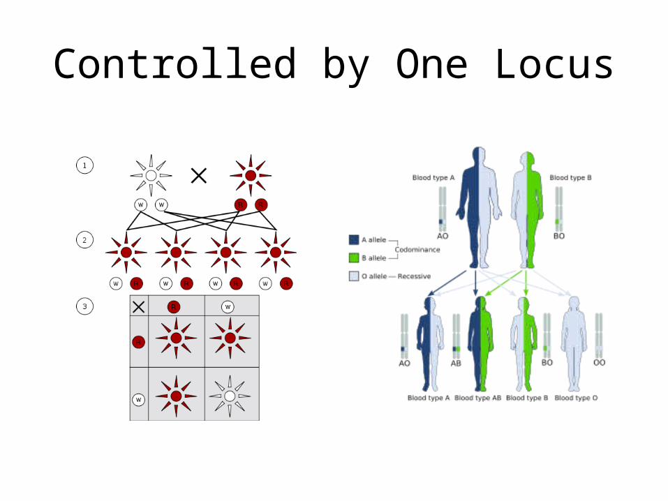
Controlled by One Locus

Donahue, R. P., et al., Probable assignment of the Duffy blood group locus to chromosome 1 in man, Proceedings of the National Academy of Sciences 61, 949-955 (1968).
Co-segregation in Pedigree

Quantitative Trait
Carlos Harjes

Trait Varies on a Continuous ScaleFr
eque
ncy
Trait Value

Quantitative Traits
• Probably caused by multiple loci– Interaction effects– Environment
If the mean trait value for individuals with marker state MM is different from the mean
trait value of individuals with marker state mm (i.e. the marker is associated with the
phenotype), then the marker is linked to a quantitative trait locus.

Mar
kers
Individuals
Trait value
Marker #3 Mean Trait Value
Present 99 ± 5
Absent 118 ± 8
Marker #6 Mean Trait Value
Present 110 ± 10
Absent 115 ± 13
Quantitative Genetics
Exploring the Genetic Architecture* Underlying Quantitative Traits
*Genetic Architecture• How many loci?• Which location?• How strong?

Tools for Statistical Genetics in the DETool Purpose
Genotype by Sequencing Workflow Automatic pipeline for extracting SNPs from GBS data (with genome from user or from iPlant database)
UNEAK pipeline Automatic pipeline for extracting SNPs from GBS data without reference genomes
MLM workflow Automatic workflow for fitting Mixed Linear Model
GLM workflow Automatic workflow for fitting General Linear Model
QTLC workflow Automatic workflow for composite interval mapping
QTL simulation workflow Automatic workflow for simulating trait data with given linkage map
PLINK PLINK implementation of various association models
Zmapqtl Interval mapping and composite interval mapping with the options to perform a permutation test
LRmapqtl Linear regression modeling
SRmapqtl Stepwise regression modeling
AntEpiSeeker Epistatic interaction modeling
Random Jungle Random Forest implementation for GWAS
FaST-LMM Factored Spectrally Transformed Linear Mixed Modeling
Qxpak Versatile mixed modeling
gluH2P Convert Hapmap format to Ped format
LD Linkage Disequilibrium plot
Structure Estimation of population structure
PGDSpider Data conversion tool
GLMstrucutre GLM with population structure as fixed effect

A Model for Quantitative Traits
P = G + E + GG + GEP=PhenotypeG=GenotypeE=EnvironmentGG=Interaction between genotypesGE=Interaction between genotype and environment
P = G + e
Phenotype
Genotype Environment

A Statistical Model for QTLs
P=G + e
yij trait value in individual j with genotype iβ0 population average of trait valueβ1 effect of marker i on trait valuexi marker genotype iεij error term
General Linear Model (in matrix notation): Y=Xb + e
Note: If errors are not normally distributed, use generalized linear models

http://concord.org/publications/newsletter/2009-spring/genetics

Linkage Mapping (QTL Mapping)
• Designed population– F2– Recombinant inbred (RIL)– Double-Haploid (DH)– Back-cross (B2)


Limitation of Linkage Mapping
• Needs large number of related individuals• Resolution limited (interval contains 100s of
genes)• QTL position and effect are confounded

Association Mapping
• Use random collection of individuals from natural population
• Very dense marker map = very high resolution

Linkage & RecombinationRecombination causes linkage decay
Other factors affecting LD:• Selection (artificial or natural)• Drift• Mutations• Population structure• Demography

Linkage Disequilibrium

Pitfalls: Population Structure
• Difference in allele frequencies between subpopulations
• Due to neutral or adaptive processes
• Can create spurious association

T G T G
No association within groups

• Similar effect due to presence of related individuals (esp. in plants)
• Can be accounted for using the data:– Estimate number of subpopulations– Assign individuals to subpopulation– Estimate kinship

Accounting for Random Effects: Mixed Linear Models
• "Cost" associated with estimating a parameter• We are not interested in the value of the parameter, only the variance• Q-K method (structured association)
y=Xβ+Sα+Qv+Zu+e
Fixed effects:β Vector of fixed effectsα Vector of SNPs effectsv Vector of subpopulation effects
Random effects:u Vector of kinship effectse Residuals
Q Matrix of population association (STRUCTURE)X, S, Z Incidence Matrices

Traits
Markers
Population Structure
Kinship
STRUCTURE
TASSEL
MLM

Obtain Markers
Genome Resequencing Workflow
Genotyping By Sequencing

MLM Pipeline for GWAS
marker
trait
filter
convert
impute
impute
K
GLM
MLM
http://www.maizegenetics.net/statistical-geneticsZhang et al. Nature Genetics. 2010; doi:10.1038/ng.546
Ed Buckler (Cornell University)TASSEL
http://www.maizegenetics.net/tassel/docs/Tassel_User_Guide_3.0.pdf

MLM Input Files
• Hapmap file• Phenotype data• Kinship matrix*• Population structure*
straintraits
Phenotype data
strain3 populations sum to 1
* Kinship matrix & population structure data can be generated using TASSEL or with “MLM Workflow” App in DE
Population structure

Origin
• Hapmap file: – Download (e.g. http://triticeaetoolbox.org/)– Convert from PLINK (.map/.ped) using Tassel 3 Conversion– Impute with NPUTE– Transform to numerical format with NumericalTransform
• Phenotype data• Kinship matrix
– Generate from hapmap marker data with Kinship• Population structure
– Generate using ParallelStructure– Convert to matrix with Structure2Tassel

MLM Output• MLM1.txt
– Marker– “df” degrees of freedom– “F” F distribution for test of marker– “p” p-value– “errordf” df used for denominator of F-test– etc.
• MLM2.txt– Estimated effect for each allele for each marker
• MLM3.txt– The compression results shows the likelihood, genetic variance, and error variance for
each compression level tested during the optimization process.
See TASSEL manual for details:http://www.maizegenetics.net/tassel/docs/Tassel_User_Guide_3.0.pdf

THANKS!
Recommended