Assessment of Relative Active Tectonics in Parts of Aravalli 1
Mountain Range, India: Implication of Geomorphic Indices, Remote 2
Sensing and GIS 3
4
Syed Ahmad Ali1*, Javed Ikbal1 5
1Department of Geology, AMU, Aligarh- 202002, India 6
[email protected] (S.A.A.) 7
[email protected] or [email protected] (J.I.) 8
*Corresponding author- Syed A. Ali 9
Department of Geology, Aligarh Muslim University, Aligarh- 202002, India, 10
Phone-+919411040526, Email- [email protected], [email protected] 11
12
Running title: Assessment of relative active tectonics in Aravalli Range, India 13
14
15
16
17
18
19
20
21
22
Preprints (www.preprints.org) | NOT PEER-REVIEWED | Posted: 2 January 2018 doi:10.20944/preprints201801.0008.v1
© 2017 by the author(s). Distributed under a Creative Commons CC BY license.

ABSTRACT: Aravalli Mountain Range is an example of erosional mountains, trending NE-SW, 23
shows numerous faults and lineaments. Udaipur area, situated south-east part of the mountain, is 24
considered as tectonically active. So the main objective is to study relative tectonic activity of the 25
Ahar watershed of Udaipur, Rajasthan, India. To assess relative tectonic activity of the area, 26
geomorphic indices such as stream length gradient index (SL), asymmetry factor (Af), basin shape 27
(Bs), valley floor width to valley height ratio (Vf), mountain front sinuosity (Smf), hypsometic 28
integral (Hi), hypsometric curve and transverse topographic symmetry factor (T) is applied. DEM 29
(SRTM), Google earth image and enhanced image of Landsat TM (2008) is used to extract linear 30
features. Result of these geomorphic indices of each sub-watersheds are used to divide area from 31
low to high relative tectonic activity classes, expressed as relative tectonic active index (Iat) and 32
according to Iat value the sub watershed UDSW2, 3 and 4 is tectonically relatively more active 33
than remaining part of the area. Field validation associated with evidences highlighted by using 34
geomorphic indices as well as stream deflrction and lineament analysis reveals that the Ahar 35
watershed of Aravalli Range, particularly the north-western flank, is most affected by tectonic 36
activity. 37
38
Keywords: geomorphic indices; relative active tectonics; stream deflection; lineament; Aravalli 39
range 40
41
42
43
44
45
Preprints (www.preprints.org) | NOT PEER-REVIEWED | Posted: 2 January 2018 doi:10.20944/preprints201801.0008.v1

1. INTERODUCTION 46
47
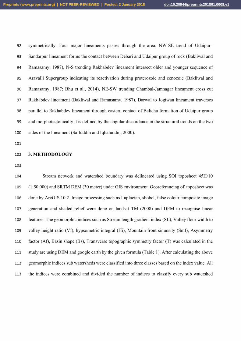
The study area is located in the northern part of Udaipur district of Rajasthan (fig 1). The 48
GPS measurements of 2007–2011 suggest that the Udaipur block moves at a rate of about 49 49
mm/year towards northeast (Bhu et al., 2014) indicating tectonically this area is active. The main 50
Ahar river passes through in this region and as the drainage network is very much influenced by 51
tectonic activity, so morphotectonic study of Ahar watershed is important to assessment the 52
tectonic activity in this area. Morphotectonic is the study of landforms produced by tectonic 53
processes. The quantitative measurements of landforms are accomplished on the basis of 54
calculation of geomorphic indices by the use of topography maps, digital elevation model٫ satellite 55
images, aerial photographs and field works (Toudeshki and Arian, 2011). Tectonic geomorphology 56
is one of the emergent disciplines in geosciences due to the advent of novel geomorphological, 57
geodetic and geochronological tools which aid the acquisition of rates (uplift rates, incision rates, 58
erosion rates, slip rates on faults, etc.) at variable time-scales (103-106 years; Burbank and 59
Anderson, 2001; Azor et al., 2002; Bull, 2007). This discipline is important because the results of 60
regional studies on neotectonics are significant for evaluating natural hazards, land use 61
development and management in populated areas (Pedrera et al., 2009). The study of tectonics 62
helps to understand about geomorphology, structural geology, stratigraphy, geochronology, 63
seismology, and geodesy. The study of the geomorphological features such as the drainage may 64
assist in understanding the landscape evolution and recognize active tectonic movements 65
(Riquelmea et al., 2003; Malik and Mohanty, 2007; Bathrellos et. al., 2009, Kamberis et al., 2012). 66
Tectonically active region influenced on drainage pattern, basin asymmetry, stream deflection, 67
river incision (Cox, 1994). The geomorphic indices are important indicators capable of decoding 68
Preprints (www.preprints.org) | NOT PEER-REVIEWED | Posted: 2 January 2018 doi:10.20944/preprints201801.0008.v1

landform responses to active deformation processes and have been widely used as a reconnaissance 69
tool to differentiate zones deformed by active tectonics (Keller and Pinter, 1996; Chen et al., 2003). 70
We use geomorphic indices of active tectonics, known to be useful in active tectonic studies (Bull 71
and McFadden, 1977; Azor et al., 2002; Silva et al., 2003; Molin et al., 2004; El Hamdouni et al., 72
2008; Mahmood and Gloaguen, 2012; Elias, 2015; Fard et al., 2015;). But this method was not 73
applied before in the study area. The main objective is to calculate different geomorphic indices 74
to assess relative active tectonics of the area. In the study area the Ahar watershed is divided into 75
10 sub watershed. Each and every sub-watershed, whether it is possible, the geomorphic indices 76
has been calculated to understand the relative tectonics. Remote sensing and field data were used 77
to analyze lithology, structure, soil erosion in the tectonically active region of Zagros mountain to 78
evaluate natural hazards like landslide (Ali et al., 2003). 79
80
2. GEOTECTONIC FRAMEWORK 81
82
This region was an active zone of sedimentation, distinct tectonism and repetitive 83
magmatism. The Banded Gneissic Complex acted as the basement during the Precambrian times 84
for the Proterozoic basins like Aravalli, Delhi (Heron, 1936). The western part of the Udaipur 85
district shows undulating topography due to NE-SW trending series of Aravalli hill. The oldest 86
formation exposed in the area belongs to Bhilwara Super group of Arachean age. The younger 87
formations of Aravalli super group and Delhi super group of Proterozoic age is found in the 88
western side of the district. Bhilwara belt and the Udaipur-Jharol belt are two major adjoining belts 89
situated in Aravalli Supergroup. The Udaipur-Jharol belt is exposed as an inverted "V" shaped area 90
with tapering end near Nathdwara. N-S trending Rakhabdev lineament divides this belt 91
Preprints (www.preprints.org) | NOT PEER-REVIEWED | Posted: 2 January 2018 doi:10.20944/preprints201801.0008.v1
symmetrically. Four major lineaments passes through the area. NW-SE trend of Udaipur–92
Sandarpur lineament forms the contact between Debari and Udaipur group of rock (Bakliwal and 93
Ramasamy, 1987), N-S trending Rakhabdev lineament intersect older and younger sequence of 94
Aravalli Supergroup indicating its reactivation during proterozoic and cenozoic (Bakliwal and 95
Ramasamy, 1987; Bhu et al., 2014), NE-SW trending Chambal-Jamnagar lineament cross cut 96
Rakhabdev lineament (Bakliwal and Ramasamy, 1987), Darwal to Jogiwan lineament traverses 97
parallel to Rakhabdev lineament through eastern contact of Balicha formation of Udaipur group 98
and morphotectonically it is defined by the angular discordance in the structural trends on the two 99
sides of the lineament (Saifuddin and Iqbaluddin, 2000). 100
101
3. METHODOLOGY 102
103
Stream network and watershed boundary was delineated using SOI toposheet 45H/10 104
(1:50,000) and SRTM DEM (30 meter) under GIS environment. Georeferancing of toposheet was 105
done by ArcGIS 10.2. Image processing such as Laplacian, shobel, false colour composite image 106
generation and shaded relief were done on landsat TM (2008) and DEM to recognise linear 107
features. The geomorphic indices such as Stream length gradient index (SL), Valley floor width to 108
valley height ratio (Vf), hypsometric integral (Hi), Mountain front sinuosity (Smf), Asymmetry 109
factor (Af), Basin shape (Bs), Transverse topographic symmetry factor (T) was calculated in the 110
study are using DEM and google earth by the given formula (Table 1). After calculating the above 111
geomorphic indices sub watersheds were classified into three classes based on the index value. All 112
the indices were combined and divided the number of indices to classify every sub watershed 113
Preprints (www.preprints.org) | NOT PEER-REVIEWED | Posted: 2 January 2018 doi:10.20944/preprints201801.0008.v1

according to relative active tectonic (Iat). Stream deflection parameter, lineament map and field 114
evidences were used to support the result come from the analysis of above geomorphic indices. 115
116
4. RESULT AND DISCUSSION 117
118
4.1 Analysis of Geomorphic Indices 119
120
Geomorphic indices including stream length gradient index (SL), valley floor width to 121
valley height ratio (Vf), hypsometric curve and hypsometric integral (Hi), Mountain front sinuosity 122
(Smf), Asymmetry factor (AF), basin shape (Bs) and transverse topographic symmetry factor (T) 123
has been analyzed and discuss on relative tectonic activity (Iat) by combination of all the 124
geomorphic parameters. 125
126
4.1.1. Stream length gradient index (SL) 127
Relative tectonic activity of an area can be appraised by using SL index. Deviation from 128
this stable river profile may be induced by tectonic, lithological and/or climatic factors (Hack, 129
1973). Soft rocks comprising high SL values is the indicators of recent tectonic activity, but low 130
values of SL in the area encompasses strike slip faults and streams are flowing through it may also 131
represent tectonically active (Keller and Pinter, 1996, Mahmood, and Gloaguen 2012). Rocks of 132
consistent resistance showing high value of stream length gradient index or fluctuation of SL 133
values indicates the area is tectonically active (Keller, 1986). The value of SL index over the study 134
area was calculated along the master stream of 10 sub-watersheds using google earth (Table 2). 135
The SL values were classified into three classes, where SL values more than 600 falls in class 1, 136
Preprints (www.preprints.org) | NOT PEER-REVIEWED | Posted: 2 January 2018 doi:10.20944/preprints201801.0008.v1
SL value in between 300 and 600 fall in class 2 and in class 3, the value of SL is less than 300 (El 137
Hamdouni et al., 2008). 138
Table 2 is about here 139
Figure 3 is about here 140
All the sub watersheds are fall in class 3 (Table 2). Relative study shows that sub watershed 141
UDSW2, UDSW3 and UDSW4 shows relatively higher SL value followed by UDSW5 and 142
UDSW8 which are relatively moderate SL value and remaining sub watersheds show low SL value 143
(Fig 5a). The relative value indicate that northern and western part of the Ahar watershed shows 144
relatively high and moderate tectonically active respectively. Eastern, southern and central part is 145
relatively tectonically less active. Places were marked where SL value relatively high and this high 146
value may be due tectonically uplifted or diverse erosion (Fig 3 ). 147
4.1.2. Ratio of Valley Floor to Valley Height (Vf) 148
The Vf index reflects the difference between V-shaped valleys that are down cut in 149
response to active uplift (low values of Vf) and broad-floored valleys that are eroding laterally into 150
adjacent hill slopes in response to base level stability (high values of Vf) (Bull, 1978). Deep V-151
shaped valleys (Vf < 1) are connected with linear, active down cutting streams distinctive of areas 152
subjected to active uplift, while flat floored (U-shaped) valleys (Vf > 1) show an attainment of the 153
base level of erosion mainly in response to relative tectonic quiescence (Keller, 1986). Vf is 154
classified into three classes: class 1 (Vf ≤ 0.5), class 2 (0.5 ≤ Vf ≤ 1.0), class 3 (Vf ≥ 1.0) (El 155
Hamdouni et al., 2008). Master stream of sub-watersheds were used to calculate the Vf values of 156
the study area (fig.). Different researcher classified Vf index with different values (El Hamdouni 157
et al., 2008; Fard et al. 2015; Mahmood and Gloagaun, 2012). In this study area Vf index is 158
classified as Class 1: (Vf<0.5), Class 2: (0.5≤Vf<1) and Class 3: (Vf≥1). Although Vf value of 159
Preprints (www.preprints.org) | NOT PEER-REVIEWED | Posted: 2 January 2018 doi:10.20944/preprints201801.0008.v1

some area shows less than 1 but the average Vf value of all the sub watersheds is more than 1 160
falling Class 3, that is flat floored U shaped valley (Table 3), but some areas mainly along the 161
lineaments, faults and mountainous region where Vf value is less than 1 indicating ‘V’ shaped 162
valley. 163
Table 3 is about here 164
4.1.3. Hypsometric Curve and Hypsometry Integral (Hi) 165
Hypsometric curve is the area-altitude relation can be described as a proportion of area 166
above each proportion in elevation. The hypsometric integral (Hi) describes the relative 167
distribution of elevation in a given area of a landscape particularly a drainage basin (Fard et al., 168
2015). The study of hypsometric curves as well as HI values provides important information about 169
tectonic behaviour of the watershed along with erosional stage of the watershed (Moglen and Bras, 170
1995; Willgoose and Hancock, 1998; Huang and Niemann, 2006). Convex-up curves having high 171
value of HI are representing youthful stage, smooth s-shaped curves crossing the center of the 172
diagram characterize mature stage, and concave-up with low HI values are indicator of old stage 173
(Strahler, 1952). Figure 4 shows the hypsometric curves of every sub watersheds. The value of 174
Maximum, minimum and mean elevation is directly taken from DEM by arc GIS software. To 175
check out the accuracy of the values particularly mean elevation data point sampling of more than 176
100 elevation values were collected from every sub watershed and computed by using DEM. 177
Figure 4 is about here 178
The value of HI index always ranges between 0 and 1 which is computed in number. Generally 179
high values of hypsometric integral shows convex hypsometric curve and low values are 180
responsible for concave curve. So on the basis of values and in respect of convexity and concavity 181
of hypsometric curve, Hypsometric integral can be classified into three classes. Class 1 (HI > 0.5 182
Preprints (www.preprints.org) | NOT PEER-REVIEWED | Posted: 2 January 2018 doi:10.20944/preprints201801.0008.v1

) shows convex hypsometric curve. Class 2 (0.4 > HI < 0.5) shows concavo-convex or straight 183
curve and class 3 (HI < 0.4) having the curve of concave shape. Hypsometric integral is convex in 184
the lower portion or low elevated area may relate to uplift along a fault or perhaps uplift associated 185
with recent folding (El Hamdouni et al., 2008). High values of the index are possibly related to 186
young active tectonic and low values are related to older landscapes that have been more eroded 187
and less impacted by recent active tectonics. The HI value in the Ahar watershed ranges from 188
0.165 (UDSW9) to 0.461 (UDSW4) (Table 4). Classification based on relative tectonic activity 189
shown (fig 5b). 190
Table 4 is about here 191
4.1.4. Mountain Front Sinuosity (Smf) 192
Smf value can be computed through topographic map or aerial photography or satellite 193
imagery and the obtain value depends on the scale of the map. Small scale map produce 194
approximate values of Smf, while large scale topographic map and aerial photography have higher 195
resolution and are more appropriate for assessment of Smf (El. Hamdauni et al., 2008). Mountain 196
front sinuosity is defined as the ratio of the length of the mountain front along the foot of the 197
mountain to the straight line length of that front (Bull, 2007; Mahmood and Gloaguen, 2012). The 198
balance between erosion that tends to produce asymmetrical or sinuous fronts and tectonic forces 199
that tend to create a straight mountain front coincident with an active range–bounding fault is 200
presented by the above mentioned index (Kokinou et.al., 2013). On the basis of tectonically 201
activeness some researchers have classified this value with tree classes. Some studies have 202
proposed that Smf values lower than 1.4 are indicative of tectonically active fronts (Rockwell et 203
al., 1985; Keller, 1986; Burbank and Anderson, 2001; Silva et al., 2003; Kokinou et al.,2013), The 204
value of Smf was computed using Lmf and Ls value measured from SRTM data with spatial 205
Preprints (www.preprints.org) | NOT PEER-REVIEWED | Posted: 2 January 2018 doi:10.20944/preprints201801.0008.v1

resolution of 30 meter in the study area. The Smf value has been classified into three classes that 206
are class 1 in which Smf<1.1, class 2 in which 1.1≤Smf<1.5 and class 3 when Smf≥1.5 (El 207
Hamdouni et al., 2008). 208
Frontal side of mountain with more than 800 meters in elevation and contour interval 209
between top of the hill or mountain and piedmont is more than 300 meter has been consider as 210
mountain front to analyse mountain front sinuosity. In the study area Smf value lies between 1.08 211
and 2.73. here sub watershed wise Smf value was consider. Instead of 1.08 of Smf value in 212
UDSW2 which is very tectonically active and fall in class 1 (El Hamdouni et al., 2008) but 213
UDSW2 has two mountain front and the average value is 1.11 (Table: ) and this sub watershed fall 214
in class 2. Mountain front sinuosity of UDSW1 and UDSW6 fall in class 3 indicate tectonically 215
less active and UDSW 2, UDSW3, UDSW4, UDSW5, UDSW7 and UDSW10 shows tectonically 216
moderately active (Table 5: and Figure: 5c). The Smf value of mountain front located lower most 217
part of the sub watershed UDSW10 is 1.05 and this low value is because this front is align along 218
with fault. 219
Table 5 is about here 220
4.1.5. Asymmetry Factor (Af) 221
Tectonic tilting with direction of tilting of drainage basin can be evaluated by the analysis 222
of Asymmetry factor at the scale of drainage basin (Sharma, et al., 2013; Siddiqui, 2014; Kale et 223
al, 2014). This method was applied over a large area (Hare and Gardner, 1985; Sboras et al.,2010). 224
Ar (area of the right side of the master stream) and At (total area of the watershed) was measured 225
by Arc Map and to calculate these parameter, looking downstream of master streams of every sub-226
watershed was considered. Af significantly greater or smaller than 50 shows influence of either 227
active tectonics or lithologic structural control or differential erosion, as for example the stream 228
Preprints (www.preprints.org) | NOT PEER-REVIEWED | Posted: 2 January 2018 doi:10.20944/preprints201801.0008.v1
slipping down bedding plains over time (El Hamdouni et al., 2008; Mahmood and Gluagoan, 229
2012). Inclination of schistocity or bedding allows for preferred migration of the valley in the 230
down-dip direction, producing an asymmetric valley (EL Hamdauni et al., 2008). The values of 231
this index are divided into three categories. 1: (Aƒ < 35 or Aƒ ≥ 65) 2: (57 ≤ Af < 65) or (35 ≤ Aƒ 232
< 43) and 3: (43 ≤ Aƒ < 57) (El Hamdouni et al, 2008). Af value in the study area ranges from 233
36.93 (UDSW4) to 59.59 (UDSW2) (Table 6). Sub watersheds UDSW2, UDSW3, UDSW4 and 234
UDSW7 falls in class 2 and the Af values of these sub watersheds indicates moderately tilting took 235
place in this area whereas remaining area falls in class 3 shows very less tectonic tilting or no 236
tilting took place in these area. Af value more than 55 and less than 45 are consider as asymmetry 237
basin and tectonic tilting were taken place towards left and right side of the basin respectively 238
while the value of Af in between 45 and 55 are considered as symmetry of the basin and the arrow 239
shows the direction of the tilting (Çağlar Özkaymak.,2015) (Fig: 5d ). Tectonic tilting of UDSW3 240
and UDSW4 are west to south west direction, UDSW7 and UDSW10 towards southern direction, 241
UDSW2 and UDSW1 are towards north-eastern and east direction respectively. 242
Table 6 is about here 243
4.1.6. Basin Shape (Bs) 244
Drainage basins with elongated in shape indicates relatively young in nature in active 245
tectonic areas. With continued evolution or less active tectonic processes, the elongated shape 246
tends to evolve to a more circular shape (Bull and McFadden, 1977) As the value of width of sub 247
watershed vary in place to place, so average value was taken to calculate basin shape. High values 248
of Bs are associated with elongated basins, generally associated with relatively higher tectonic 249
activity and Low values of Bs indicate a more circular-shaped basin, generally associated with low 250
Preprints (www.preprints.org) | NOT PEER-REVIEWED | Posted: 2 January 2018 doi:10.20944/preprints201801.0008.v1

tectonic activity (El Hamdouni et al., 2008). Bs index can be classified as Class 1: (Bs≥4), Class 251
2: (3≤Bs≥4) and class 3: (Bs≤3) (El Hamdouni et al., 2008) (Fig: 5e). 252
Bs value ranges from 1.51 (UDSW1) to 4.71 (UDSW2) (Table: 7). Only UDSW2, UDSW4 and 253
UDSW9 have Bs index is just above 4 which reveals the watersheds is elongated in nature and 254
tectonically highly active. Bs index of UDSW3 is just above 3 and falls in class 2 indicates 255
elongated to sub elongated in nature and tectonically moderately active. Remaining part of the 256
study area has Bs value less than 3 or it can be say more or less close to 2, which indicates these 257
sub watershed shows more circular in nature and tectonically less active region. 258
Table 7 is about here 259
4.1.7. Transverse Topographic Symmetry Factor (T) 260
Neotectonic activity of an area can be identified by the study of drainage basin asymmetry 261
although the active structures are poorly exposed or covered by quaternary alluvium (Cox et al, 262
2001). If there is no tectonic activity occurs, then the main river will flow evenly from both sides 263
as a perfect symmetric basin and the value of T will be zero. The T value varies from 0 to 1 264
depending upon the intensity of the tectonic activity. Values near to 1.0 indicate that the river flows 265
closely to the margins of the basin, a result probably produced by intensive and recent tectonic 266
activity. Values of T were calculated to assess the migration of streams perpendicular to the 267
drainage basin axis (Keller & Pinter 1996). 268
Table 8 is about here 269
The value of T for all the sub watersheds is determined and the results are presented (Table: 270
8). Position of the T value which has been calculated is also shown (Fig: 5f). A number of segments 271
in each sub watershed has been considered to determine T value and average value is taken to 272
understand asymmetrical behaviour of sub watershed. T value ranges from 0.05 (almost symmetry) 273
Preprints (www.preprints.org) | NOT PEER-REVIEWED | Posted: 2 January 2018 doi:10.20944/preprints201801.0008.v1
to 0.47 (asymmetry). Transverse topographic symmetry factor can be classified into three classes 274
such as Class 1 for T > 0.4, class 2 for T between 0.2 and 0.4 and class 3 for T < 0.2 (Mosavi and 275
Arian, 2015). Sub watershed situated western part of the study area has T value more than 0.4 (fig 276
5f) showing asymmetry in nature indicates these area falls under tectonically highly active. 277
UDSW7 and UDSW8 of the western part of the study area has T value 0.18 (class 3) and 0.32 278
(class 2) respectively indicating tectonically less active and moderately active. UDSW6 falls in 279
class 2 with T value 0.32 and T value of UDSW1 has 0.18 and falls in class 3. 280
Figure 5 is about here 281
4.1.8. Discussion on Relative Tectonic Activity (Iat) 282
Aravalli is an example of erosional mountain. Udaipur is situated south-east part of the 283
mountain, is consider as tectonically active. So here the main objective is to study relative tectonic 284
activity of the study area. Several studies describe about relative tectonic activities by the use of 285
combination of Smf and Vf indexes in such a manner that the Vf values are plotted with the Smf 286
values on a same diagram in order to produce a relative degree of tectonic activity and recognition 287
of three different classes (Bull and McFadden, 1977; Silva et al., 2003; Kokinou et al., 2013). 288
Several studies shows the relative tectonic activity (Iat) with the help of seven geomorphic indices 289
(Sl, Vf, Smf, HI, Af, Bs, T) which is applied here (El. Hamdouni et al., 2008; Fard et al., 2015; 290
Elias, 2015; Mosavi and Arian, 2015). Every geomorphic indices has been classified into three 291
classes in which class 1 and class 3 represents high and low tectonically active respectively. 292
Table 9 is about here 293
Iat is obtained by the average of the different classes of geomorphic indices (S/n) and 294
divided into four classes, where class 1 is very high tectonic activity with values of S/n between 1 295
and 1.5; class 2 is high tectonic activity with values of S/n≥1.5 but < 2; class 3 is moderately active 296
Preprints (www.preprints.org) | NOT PEER-REVIEWED | Posted: 2 January 2018 doi:10.20944/preprints201801.0008.v1

tectonics with S/n≥2 but < 2.5; and class 4 is low active tectonics with values of S/n≥2.5 (El. 297
Hamdouni et al., 2008). The average value of class of geomorphic indices of the active tectonics 298
(S/n) and the relative tectonic activity index value (Iat) are summarized (Table: 9). Iat index class 299
of UDSW2, UDSW3 and UDSW4 is 3 which reveals that northern part of the study area shows 300
moderately tectonic active area, whereas rest of the study area where Iat index class is 4 falls under 301
comparatively less tectonic active area (Fig: 6a). Within the study area 89.89 Km2 i.e. 20.56% of 302
the total area is class 3 measured by Iat which is moderately tectonically active. 347.41 Km2 or 303
79.44% of the area is class 4 measured by Iat is tectonically less active. 304
Figure 6 is about here 305
4.2. Stream Deflection 306
307
Sudden change of stream flow direction is atream anomaly occurs may be due to tectonic 308
geomorphology such as fault or fold or may be due to sub surface structure or lithological change. 309
Thus stream network analysis is a fundamental tool in tectonic geomorphology (Deffontaines and 310
Chorowich, 1991). Defflection of channel occurs when it crosses through fault because the 311
variation of erosion took place in fault zone. 312
Encircled area showing anomalies i.e. deflection of the flow direction of stream channel (Fig: 6b). 313
In the encircled area of sub watershed UDSW10, stream suddenly changed its direction from SE 314
to NE with angle of 85o due to fault is present there. In the area A3 and A4, the stream flows 315
towards NNE and suddenly changed its direction towards NE and towards east making angle 65o 316
and 70o respectively. At point encircled A1 stream has changed its direction from SE to towards 317
east with an angle 67o. In the area A2, stream flow towards south parallel to mountain front and 318
changed its direction and suddenly changed its direction with 120o and moves towards NE along 319
Preprints (www.preprints.org) | NOT PEER-REVIEWED | Posted: 2 January 2018 doi:10.20944/preprints201801.0008.v1

the Chambal-Jamnagar lineament. Interestingly 3.8 Km apart from the point of deflection towards 320
NE (same direction of the stream after changed its direction) there is a fault and the trend of the 321
fault is NE-SW. Encircled A2 and A3 shows after deflection the stream moves towards NE and 322
making nearly linear or curvilinear with the fault. . 323
The stream capture and beheaded streams, features are widely recognise as a typical geomorphic 324
illustation of tectonic structure such as fault or fold (Schumm, 1977) are observed at many places 325
and has been used to draw an extensive fault (Shabir et al., 2013). So further study is needed to 326
say that either the fault is extended uppto the western point of the lineation or not. Stream 327
deflections are identified in the mountain front zone which are may be the occurence of possible 328
geological structure and the sherp bends are used as evidence of presence of tectonic structure. 329
330
4.3. Lineament 331
332
Lineament mapping is valuable component to understand the tectonic behavior of the area 333
(Kassou et al., 2012). Dominant lineament direction can give the idea about the regional fracture 334
pattern of an area (McElfresh et al., 2002, Casas et al., 2000, Koike et al., 1998). Linear geological 335
structures of seismogenic compressional setting were identified through FCC, edge enhancement 336
filters and DEM derived product to understand tectonic behavior of the area and evaluate the 337
compressional direction (Ali and Ali, 2017). The high density lineament observed towards western 338
side of the area (Fig 7a). Rose diagram shows that the orientation of lineament distribution of the 339
area (Fig 7b). The main direction is N-S followed by NE-SW and NW-SE. small amount of E-W 340
direction is also present. The lineament map also indicate that the present day stream network is 341
influenced by the lineament direction (fig 7c). 342
Preprints (www.preprints.org) | NOT PEER-REVIEWED | Posted: 2 January 2018 doi:10.20944/preprints201801.0008.v1

Figure 7 is about here 343
344
FIELD EVIDENCES 345
346
Abundant evidence of vertical displacement and numerous rock deformations observed 347
here but interpretation of active tectonic is difficult due to lack of absolute date of displacement. 348
Mainly Archean and Proterozoic rocks are covered the whole area but Quaternary and recent 349
alluvium overlies in isolated patches, along river courses and in the shallow depression (CGWB 350
report, 2013). A major crack or may be fault has been found in the field but did not identify the 351
movement (Fig 8a). In zoom in position of that figure, roots without plant can be seen along the 352
crack because by removing of mass, plant also has been removed. This fifure reveals that the crack 353
has been developed after plantation which is quaternary or recent geological age. Sudden 354
deflection of river channel of nearly right angle (fig 8b), straight river course (fig 8c), triangular 355
facet (fig 8d), soft rock deformation (fig 8e), displacement and movement of lineament (fig. 8g), 356
straight mountain front (fig 8h) are some evidences that express as active tectonic. Fig 8f shows 357
straight river course and at the position of yellow circle the river got high meandering. This 358
meandering may be due to tectonic upliftment indicating active tectonics. 359
Figure 8 is about here 360
361
CONCLUSION 362
363
Study of seismic event confirms that Udaipur district falls under seismically low damage 364
risk zone. SL value and Vf value shows all the sub watershed falls in class 3 indicates tectonically 365
Preprints (www.preprints.org) | NOT PEER-REVIEWED | Posted: 2 January 2018 doi:10.20944/preprints201801.0008.v1
less active. But in some places along the master streams of sub watershed belongs to the western 366
side of the study area shows V-shaped valley and also high SL value as more than 1000. 367
Fluctuation of SL value in the western side indicates tectonically relatively more active than 368
eastern side. Values of HI, AF and Bs show that UDSW2, UDSW3 and UDSW4 are tectonically 369
more active relative to others. By the study of Smf and T value, western part of the watershed is 370
tectonically more active. Comparing all the geomorphic indices or Iat value indicates 20.56% of 371
the total area mainly north western part of the study area is tectonically more active than remaining 372
79.44% area. Field evidences of abnormal geomorphic impression, high lineament density and 373
sudden change of stream direction found on the western side of the watershed which strongly 374
supports the above statements. 375
376
REFERENCES 377
378
Ali, S. A., Rangzan, K., Pirasteh, S., 2003, Use of digital elevation model for study of drainage 379
morphometry and identification stability and saturation zones in relation to landslide 380
assessments in parts of Shahbazan area, SW Iran. Cartography, 32 (2), 71-76 381
Ali, S. A. And Ali, U., 2017, Evaluating linear geological structures in seismogenic compressional 382
setting, Kashmir basin, NW-Himalaya. Spatial Information Research, 25 (6), 801-811. 383
Azor, A., Keller, E.A. and Yeats, R.S., 2002, Geomorphic indicators of active fold growth: Oak 384
Ridge anticline, Ventura basin, southern California. GSA Bulletin, 114, 745-753. 385
Bathrellos, G. D., Antoniou, V. E. and Skilodimou, H. D., 2009, Morphotectonic characteristics 386
of Lefkas Island during the Quaternary (Ionian Sea, Greece). Geologica Balcanica, 38 (1–387
3), 23–33. 388
Preprints (www.preprints.org) | NOT PEER-REVIEWED | Posted: 2 January 2018 doi:10.20944/preprints201801.0008.v1

Bhu, H., Purohit, R., Ram, J., Sharma, P. and Jakhar, S.R., 2014, Neotectonic activity and parity 389
in movements of Udaipur block of the Arvalli Craton and Indian Plate. Journal of Earth 390
System Science, 123, 2, pp. 343–350. 391
Bakliwal, P.C., and Ramasamy, S.M., 1987, Lineament fabric of Rajasthan and Gujarat. 392
Geological Survey of India, 113(7), 54-64. 393
Bull, W. and McFadden L., 1977, Tectonic geomorphology north and south of the Garlock Fault, 394
California. In: Doehring, D. O. (eds.), Geomorphology in arid regions. Geomorphology, 395
State University of New York at Bingamton, pp. 115–138. 396
Bull, W.B., 1978, Geomorphic Tectonic Classes of the South Front of the San Gabriel Mountains, 397
California. U.S. Geological Survey Contract Report, 14-08-001-G-394, Office of 398
Earthquakes, Volcanoes and Engineering, Menlo Park, Calif, pp-59 399
Bull, W.B., 2007, Tectonic Geomorphology of Mountains: A NewApproach to Paleoseismology. 400
Wiley-Blackwell, Oxford, 328 pp. 401
Burbank, D.W. and Anderson, R.S., 2001, Tectonic Geomorphology. Blackwell Science, Oxford, 402
247 pp. 403
Chen, Y.C., Sung, Q.C. and Cheng, K.Y., 2003, Along-strike variations of morphotectonic features 404
in the western foothills of Taiwan: tectonic implications based on stream gradient and 405
hypsometric analysis. Geomorphology 56, 109-137. 406
Cox, R. T., 1994, Analysis of drainage basin symmetry as a rapid technique to identify areas of 407
possible quaternarytilt block tectonics: an example from the Mississippi embayment. 408
Geological Society American Bulletin, 106, 571-581. doi:10.1130/0016 409
7606(1994)106<0571:AODBSA>2.3.CO;2 410
Preprints (www.preprints.org) | NOT PEER-REVIEWED | Posted: 2 January 2018 doi:10.20944/preprints201801.0008.v1
Cox, R. T., Van Arsdale, R. B. and Harris, J. B., 2001, Identification of possible Quaternary 411
deformation in the northwestern Mississippi Embayment using quantitative geomorphic 412
analysis of drainage basin asymmetry. Geological Society of America Bulletin, 113, 615–413
624. 414
Çağlar Özkaymak, 2015, Tectonic analysis of the Honaz Fault (western Anatolia) using 415
geomorphic indices and the regional implications. Geodinamica Acta, 27:2-3, 110-129, 416
DOI: 10.1080/09853111.2014.957504. http://dx.doi.org/10.1080/09853111.2014.957504 417
Deffontaines, B.,and Chorowich, J., 1991, Principle of drainage basin analysis from multisource 418
data: application to the structural analysisof the Zaire basin. Tectonophysics, 194, 237-263. 419
El Hamdouni, R., Irigaray, C., Fernández, T., Chacón, J. and Keller, E.A., 2008, Assessment of 420
relative active tectonics, southwest border of Sierra Nevada (Southern Spain). 421
Geomorphology, 96, 150-173. http://dx.doi.org/10.1016/j.geomorph.2007.08.004 422
Elias, Z., 2015, The Neotectonic Activity Along the Lower Khazir River by Using SRTM Image 423
and Geomorphic Indices. Earth Sciences, 1(1), 50-58. doi:10.11648/j.earth.20150401.15 424
Fard, N.G., Sorbi, A. and Arian, M., 2015, Active Tectonics of Kangavar Area, West Iran. Open 425
Journal of Geology, 5, 422-441. http://dx.doi.org/10.4236/ojg.2015.56040 426
Hack, J.T., 1973. Stream-profiles analysis and stream-gradient index. Journal of Research of the 427
U.S. Geological Survey, 1 (4), 421–429. 428
Hare, P.W. and Gardner, T.W., 1985, Geomorphic indicators of vertical neotectonism along 429
converging plate margins, Nicoya Peninsula, Costa Rica. In: Morisawa, M., Hack, J.T. 430
(Eds.), Tectonic Geomorphology. Proceedings of the 15th Annual Binghamton 431
Geomorphology Symposium. Allen and Unwin, Boston, MA, pp. 123–134. 432
Preprints (www.preprints.org) | NOT PEER-REVIEWED | Posted: 2 January 2018 doi:10.20944/preprints201801.0008.v1

Heron, A.M. (1936). The Geology of South Eastern Mewar. Memoir Geological Survey of India, 433
68(1), 1-120. 434
Huang, X.J., and Niemann, J.D., 2006, Modelling the potential impacts of groundwater hydrology 435
on longterm drainage basin evolution. Earth Surface Processes and Landforms, 31, 1802–436
1823. 437
Kamberis, E., Bathrellos, G. D., Kokinou, E. and Skilodimou, H. D., 2012, Correlation between 438
the structural pattern and the development of the hydrographic network in a portion of the 439
Western Thessaly Basin (Greece); Central Europian Journal of Geosciences. 4(3) 416–424. 440
Kassou, A., Essahlaoui, A. and Aissa, M., 2012, Extraction of Structural Lineaments from Satellite 441
Images Landsat7 ETM+ of Tighza Mining District (Central Morocco), Research Journal 442
of Earth Sciences, 4 (2), 44-48 443
Kele, V.S., Sengupta, S.,Achyuthan, H. And Jaiswal, M.K., 2014, Tectonic controls upon Kaveri 444
River drainage, cratonic peninsular India: Inferences from longitudinal profiles, 445
morphotectonic indices, hanging valley and fluvial records. Geomorphology, 227, 153-165 446
Keller, E.A., 1986, Investigation of active tectonics: use of surficial Earth processes. In: Wallace, 447
R. E., (Eds.), Active Tectonics, Studies in Geophysics. National Academy Press, 448
Washington, DC, pp. 136–147. 449
Keller, E.A., Pinter, N., 1996, Active Tectonics: Earthquakes, Uplift, and Landscape, Prentice 450
Hall, Inc., New Jersey, p.121-205. 451
Kokinou, E., Skilodimou H. D. and Bathrellos G.D., 2013, Morphotectonic analysis of Heraklion 452
Basin (Crete, Greece). Bulletin of the Geological Society of Greece, Proceedings of the 453
13th International Congress, Chania. September, 2013, vol. XLVII, No. 1, pp- 285-294, 454
Preprints (www.preprints.org) | NOT PEER-REVIEWED | Posted: 2 January 2018 doi:10.20944/preprints201801.0008.v1

Mahmood, S.A., and Gloaguen, R., 2012, Appraisal of active tectonics in Hindu Kush: Insights 455
from DEM derived geomorphic indices and drainage Analysis. Geoscience Frontiers, 3(4), 456
407-428. doi:10.1016/j.gsf.2011.12.002 457
Malik, J.N. and Mohanty, C., 2007, Active tectonic influence on the evolution of drainage and 458
landscape: Geomorphic signatures from frontal and hinterland areas along the 459
Northwestern Himalaya, India. Journal of Asian Earth Sciences, 29, 604–618. 460
doi:10.1016/j.jseaes.2006.03.010. 461
Moglen, G.E. and Bras, R.L., 1995, The effect of spatial heterogeneities on geomorphic expression 462
in a model of basin evolution. Water Resources Research, 31, 2613–2623. 463
Molin, P., Pazzaglia, F.J. and Dramis, F., 2004, Geomorphic Expression of Active Tectonics in a 464
Rapidly-Deforming Forearc, Sila Massif, Calabria, Southern Italy. American Journal of 465
Science, 304, 559-589. http://dx.doi.org/10.2475/ajs.304.7.559 466
Mosavi, E. J. and Arian, M., 2015, Neotectonics of Kashaf Rud River, NE Iran by Modified Index 467
of Active Tectonics (MIAT). International Journal of Geosciences, 6, 776-794. 468
http://dx.doi.org/10.4236/ijg.2015.67063 469
Pedrera, A., P_erez-Pe~na, J.V., Galindo-Zald_ıvar, J., Aza~n_on, J.M. and Azor, A., 2009, 470
Testing the sensitivity of geomorphic indices in areas of low-rate active folding (eastern 471
Betic Cordillera, Spain). Geomorphology, 105, 218-231. 472
Riquelmea, R., Martinod, J., Herail, G., Darrozesa, J. and Charrierb, R., 2003, A geomorphological 473
approach to determining the Neogene to Recent tectonic deformation in the Coastal 474
Cordillera of northernChile (Atacama), Tectonophysics, 361, 255–275. 475
Rockwell, T. K., Keller, E.A. and Johnson, D.L., 1985, Tectonic geomorphology of alluvial fans 476
and mountain fronts near Ventura, California. In: Morisawa, M. (Ed.), Tectonic 477
Preprints (www.preprints.org) | NOT PEER-REVIEWED | Posted: 2 January 2018 doi:10.20944/preprints201801.0008.v1

Geomorphology. Proceedings of the 15th Annual Geomorphology Symposium. Allen and 478
Unwin Publishers, Boston, MA, pp. 183–207. 479
Saifuddin and Iqbaluddin, 2000, Thrust controlled lineaments of the Aravalli-Delhi fold belt, 480
Rajasthan, India mapped from Landsat TM image. Journal of the Indian society of Remote 481
Sensing, 28, 47-58 482
Sboras S., Ganas A. and Pavlides S., 2010, Morphotectonic analysis of the neotectonic and active 483
faults of Berotia (central Greece) using GIS techniques. Bulletin of the Geological society 484
of Greece, Proceedings of the 12th International congress, Patras. Vol. XLIII, No. 3, pp- 485
1607-1618. 486
Schumm, S.A., 1977, The fluvial system. John Wiley, New York, p-338. 487
Siddiqui, S., 2014, Appraisal of active deformation using DEM-based morphometric indices 488
analysis in Emilia-Romagna Apennines, Northern Italy. Geodynamics research 489
international bulletin, 1(3), pp- XXXIV-XLII. 490
Silva, P. G., Goy, J. L., Zazo, C. and Bardaji, T., 2003, Faultgenerated mountain fronts in south-491
east Spain: Geomorphologic assessment of tectonic and seismic activity. Geomorphology, 492
50, 203–225. http://dx.doi.org /10.1016/S0169-555X(02)00215-5. 493
Strahler, A. N., 1952, Hypsometric (area-altitude) analysis of erosional topology. Geological 494
Society of America Bulletin, 63 (11), 1117–1142 495
Toudeshki, V.H. and Arian, M., 2011, Morphotectonic Analysis in the GhezelOzan River Basin, 496
NW Iran. Journal of Geography and Geology, 3, 258-260. 497
Willgoose and Hancock, G., 1998, Revisiting the hypsometric curve as an indicator of form and 498
process in transport-limited catchment. Earth Surface Processes and Landforms, 23, 611–499
623. 500
Preprints (www.preprints.org) | NOT PEER-REVIEWED | Posted: 2 January 2018 doi:10.20944/preprints201801.0008.v1

LIST OF TABLES AND FIGURES 501
502
Table 1. Formula of different geomorphic indices 503
Table 2. Sub watershed wise average SL value with class 504
Table 3. Vf value with classification of sub watershed 505
Table 4. Sub watershed wise Hi with classification 506
Table 5. Sub watershed wise Smf value with classification 507
Table 6. Sub watershed wise AF value with classification 508
Table 7. Sub watershed wise Bs value with classification 509
Table 8. Sub watershed wise T value with classification 510
Table 9. Relative tectonic activity classification 511
512
Fig. 1. Location map of the study area. 513
Fig. 2. Geological map of the study area. 514
Fig. 3. Graph showing SL index with respect to stream profile and the exact position of anomalies 515
area were marked with the help of Google earth image. 516
Fig. 4. Sub watershed wise Hypsometric curve 517
Fig. 5. Classification based on different geomorphic indices (a) SL index (b) HI index (c) Smf (d) 518
AF (e) Bs (f) T 519
Fig. 6. (a) Relative tectonic activity (b) Stream deflection 520
Fig. 7. Lineament map (a) density of lineament (b) rose diagram shows orientation of lineament 521
and (c) lineament map with stream network 522
Fig. 8. Field evidences of active tectonics 523
Preprints (www.preprints.org) | NOT PEER-REVIEWED | Posted: 2 January 2018 doi:10.20944/preprints201801.0008.v1

Table 1. Formula of different geomorphic indices 524
Parameter Formula References
Stream length gradient Index
(SL)
SL = (dH/dL)*L Hack, 1973
Ratio of valley floor to valley
height (Vf)
Vf = 2Vfw/ [(Eld – Esc) +
(Erd – Esc)]
Bull, 1977, 1978
Hypsometry integral (HI) HI = (Elev mean – Elev min) /
(Elev max – Elev min)
Pike and Wilson 1971
Mountain front sinuosity
(Smf)
Smf = Lmf / Ls Bull and McFadden, 1977
Asymmetry factor AF = (Ar / At) × 100 Hare and Gardner 1985
Basin shape (Bs) Bs = Bl / Bw Bull and McFadden, 1977
Transverse topographic
symmetry factor (T)
T=Da/Dd Cox, 1994
525
Preprints (www.preprints.org) | NOT PEER-REVIEWED | Posted: 2 January 2018 doi:10.20944/preprints201801.0008.v1
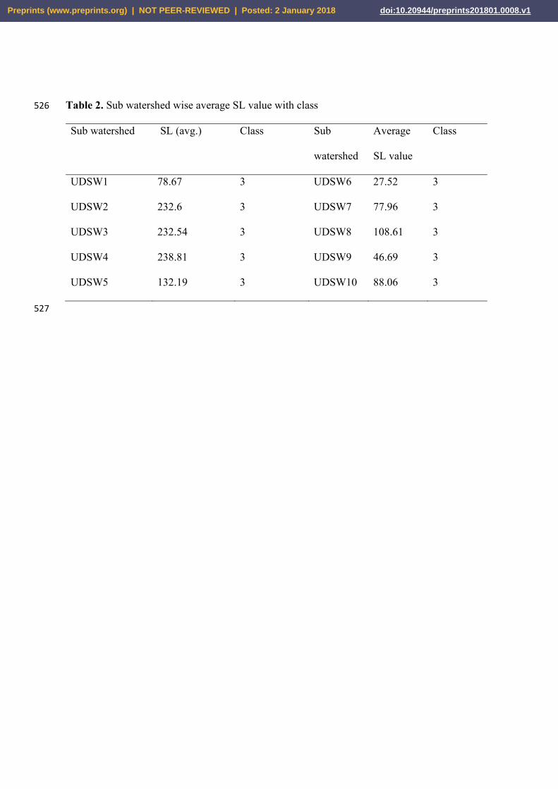
Table 2. Sub watershed wise average SL value with class 526
Sub watershed SL (avg.) Class Sub
watershed
Average
SL value
Class
UDSW1 78.67 3 UDSW6 27.52 3
UDSW2 232.6 3 UDSW7 77.96 3
UDSW3 232.54 3 UDSW8 108.61 3
UDSW4 238.81 3 UDSW9 46.69 3
UDSW5 132.19 3 UDSW10 88.06 3
527
Preprints (www.preprints.org) | NOT PEER-REVIEWED | Posted: 2 January 2018 doi:10.20944/preprints201801.0008.v1
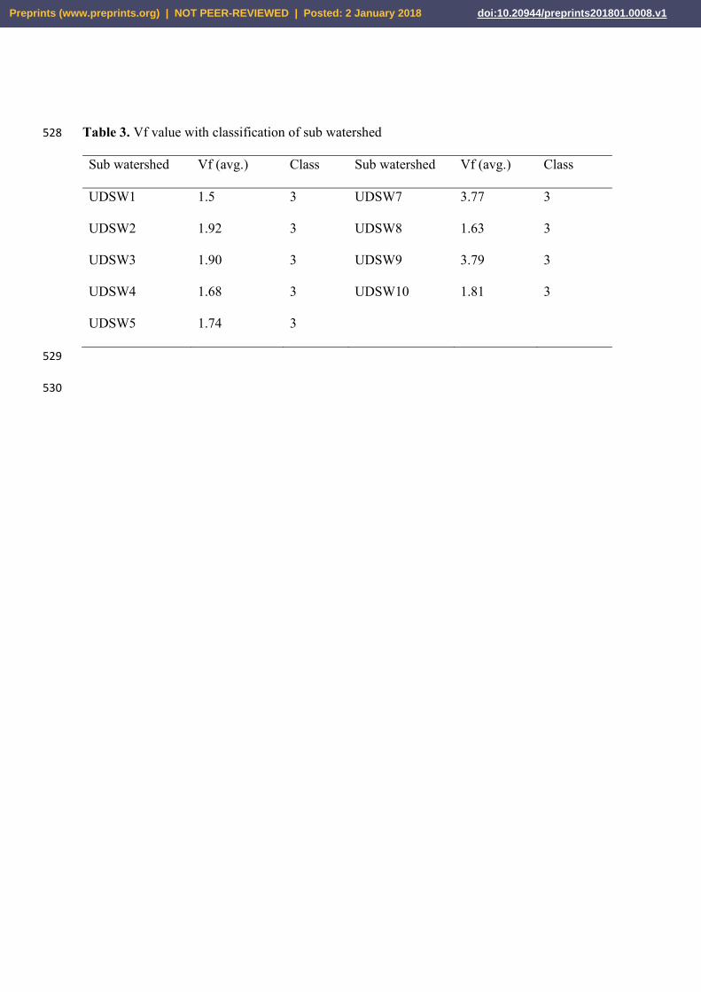
Table 3. Vf value with classification of sub watershed 528
Sub watershed Vf (avg.) Class Sub watershed Vf (avg.) Class
UDSW1 1.5 3 UDSW7 3.77 3
UDSW2 1.92 3 UDSW8 1.63 3
UDSW3 1.90 3 UDSW9 3.79 3
UDSW4 1.68 3 UDSW10 1.81 3
UDSW5 1.74 3
529
530
Preprints (www.preprints.org) | NOT PEER-REVIEWED | Posted: 2 January 2018 doi:10.20944/preprints201801.0008.v1
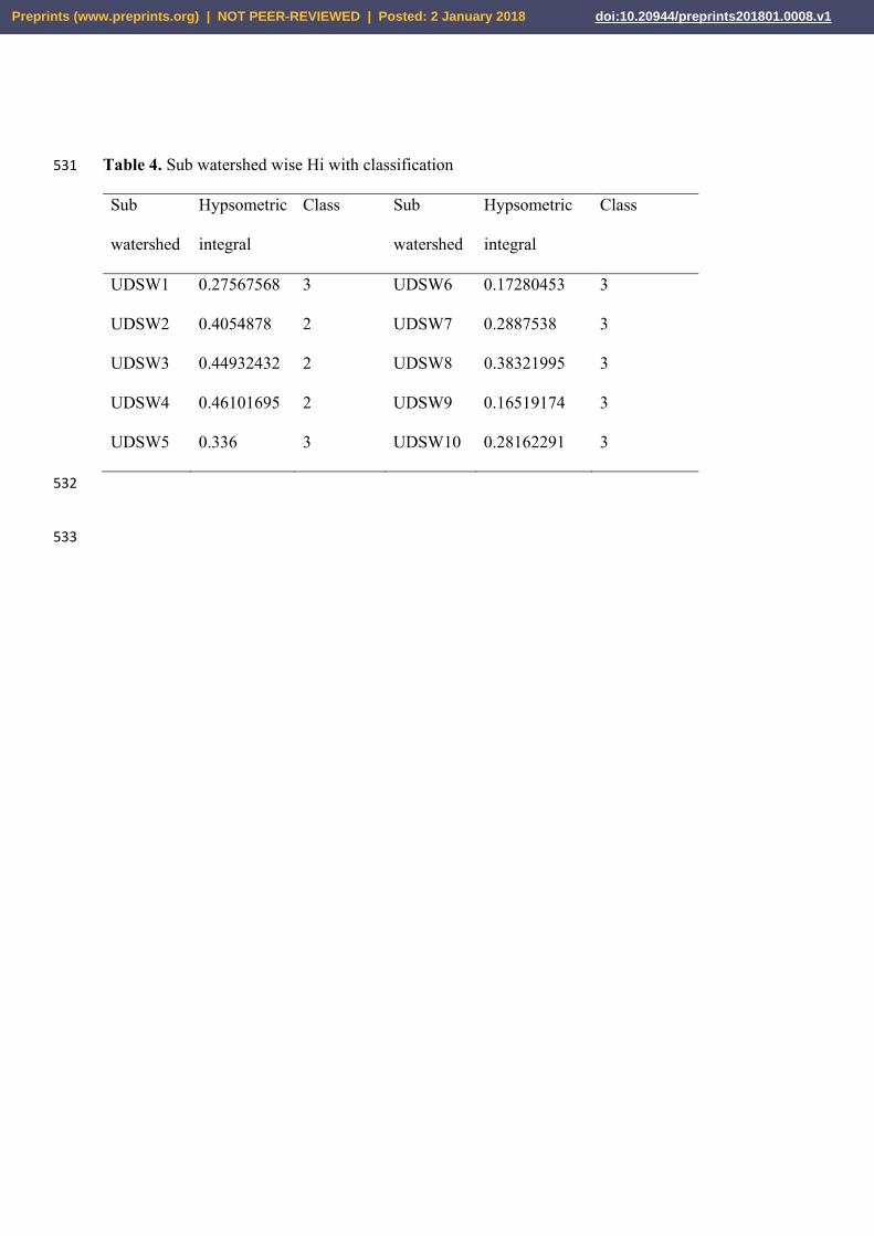
Table 4. Sub watershed wise Hi with classification 531
Sub
watershed
Hypsometric
integral
Class Sub
watershed
Hypsometric
integral
Class
UDSW1 0.27567568 3 UDSW6 0.17280453 3
UDSW2 0.4054878 2 UDSW7 0.2887538 3
UDSW3 0.44932432 2 UDSW8 0.38321995 3
UDSW4 0.46101695 2 UDSW9 0.16519174 3
UDSW5 0.336 3 UDSW10 0.28162291 3
532
533
Preprints (www.preprints.org) | NOT PEER-REVIEWED | Posted: 2 January 2018 doi:10.20944/preprints201801.0008.v1

Table 5. Sub watershed wise Smf value with classification 534
Sub watershed Lmf (KM) Ls (KM) Smf Class
UDSW1 4.34 1.83 2.73 2.03 3
4.15 3.11 1.33
UDSW2 2.74 2.40 1.14 1.11 2
1.38 1.27 1.08
UDSW3 3.12 2.17 1.44 2
UDSW4 7.23 5.09 1.42 2
UDSW5 6.07 5.06 1.19 2
UDSW6
13.96 8.69 1.60
1.65
3
8.39 4.59 1.82
4.19 2.88 1.45
3.76 2.54 1.48
2.02 1.06 1.90
UDSW7 3.25 2.59 1.25 2
UDSW10 4.46 3.08 1.45 1.25 2
4.35 4.11 1.05
535
536
Preprints (www.preprints.org) | NOT PEER-REVIEWED | Posted: 2 January 2018 doi:10.20944/preprints201801.0008.v1
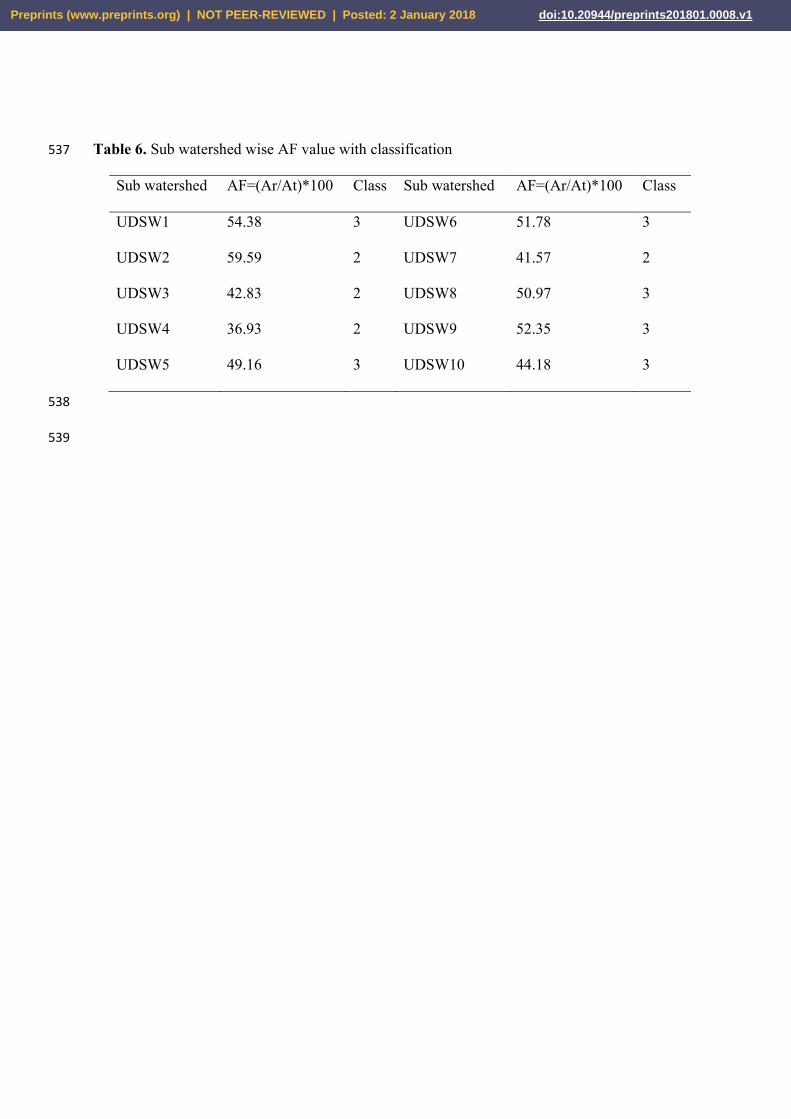
Table 6. Sub watershed wise AF value with classification 537
Sub watershed AF=(Ar/At)*100 Class Sub watershed AF=(Ar/At)*100 Class
UDSW1 54.38 3 UDSW6 51.78 3
UDSW2 59.59 2 UDSW7 41.57 2
UDSW3 42.83 2 UDSW8 50.97 3
UDSW4 36.93 2 UDSW9 52.35 3
UDSW5 49.16 3 UDSW10 44.18 3
538
539
Preprints (www.preprints.org) | NOT PEER-REVIEWED | Posted: 2 January 2018 doi:10.20944/preprints201801.0008.v1

Table 7. Sub watershed wise Bs value with classification 540
Sub watershed Bs=Bl/Bw Class Sub watershed Bs=Bl/Bw Class
UDSW1 1.51 3 UDSW6 1.95 3
UDSW2 4.07 1 UDSW7 1.98 3
UDSW3 3.07 2 UDSW8 2.01 3
UDSW4 4.71 1 UDSW9 4.09 1
UDSW5 1.95 3 UDSW10 1.67 3
541
542
Preprints (www.preprints.org) | NOT PEER-REVIEWED | Posted: 2 January 2018 doi:10.20944/preprints201801.0008.v1

Table 8. Sub watershed wise T value with classification 543
Sub watershed T=Da/Dd (avg.) class Sub watershed T=Da/Dd (avg.) class
UDSW1 0.18 3 UDSW6 0.32 2
UDSW2 0.42 1 UDSW7 0.18 3
UDSW3 0.41 1 UDSW8 0.32 2
UDSW4 0.47 1 UDSW9 0.05 3
UDSW5 0.47 1 UDSW10 0.41 1
544
545
Preprints (www.preprints.org) | NOT PEER-REVIEWED | Posted: 2 January 2018 doi:10.20944/preprints201801.0008.v1
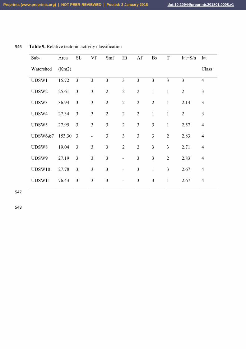
Table 9. Relative tectonic activity classification 546
Sub-
Watershed
Area
(Km2)
SL Vf Smf Hi Af Bs T Iat=S/n Iat
Class
UDSW1 15.72 3 3 3 3 3 3 3 3 4
UDSW2 25.61 3 3 2 2 2 1 1 2 3
UDSW3 36.94 3 3 2 2 2 2 1 2.14 3
UDSW4 27.34 3 3 2 2 2 1 1 2 3
UDSW5 27.95 3 3 3 2 3 3 1 2.57 4
UDSW6&7 153.30 3 - 3 3 3 3 2 2.83 4
UDSW8 19.04 3 3 3 2 2 3 3 2.71 4
UDSW9 27.19 3 3 3 - 3 3 2 2.83 4
UDSW10 27.78 3 3 3 - 3 1 3 2.67 4
UDSW11 76.43 3 3 3 - 3 3 1 2.67 4
547
548
Preprints (www.preprints.org) | NOT PEER-REVIEWED | Posted: 2 January 2018 doi:10.20944/preprints201801.0008.v1
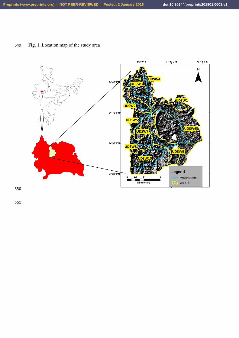
Fig. 1. Location map of the study area 549
550
551
Preprints (www.preprints.org) | NOT PEER-REVIEWED | Posted: 2 January 2018 doi:10.20944/preprints201801.0008.v1

Fig. 2. Geological map of the study area. 552
553
554
Preprints (www.preprints.org) | NOT PEER-REVIEWED | Posted: 2 January 2018 doi:10.20944/preprints201801.0008.v1
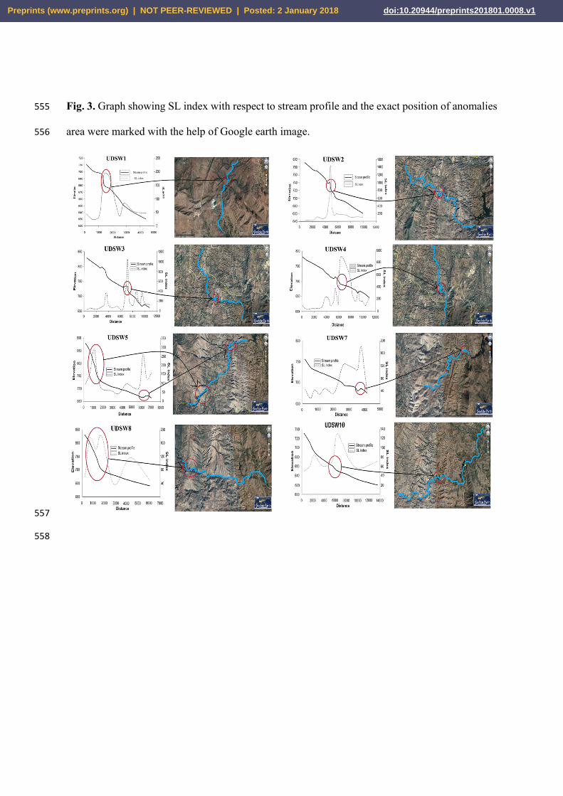
Fig. 3. Graph showing SL index with respect to stream profile and the exact position of anomalies 555
area were marked with the help of Google earth image. 556
557
558
Preprints (www.preprints.org) | NOT PEER-REVIEWED | Posted: 2 January 2018 doi:10.20944/preprints201801.0008.v1
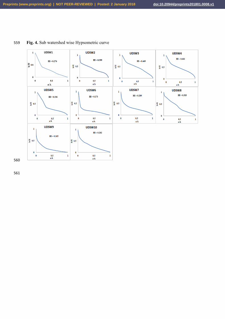
Fig. 4. Sub watershed wise Hypsometric curve 559
560
561
Preprints (www.preprints.org) | NOT PEER-REVIEWED | Posted: 2 January 2018 doi:10.20944/preprints201801.0008.v1

Fig 5. Classification based on different geomorphic indices (a) SL index (b) HI index (c) Smf (d) 562
AF (e) Bs (f) T 563
564
565
Preprints (www.preprints.org) | NOT PEER-REVIEWED | Posted: 2 January 2018 doi:10.20944/preprints201801.0008.v1

Fig 6. (a) Relative tectonic activity (b) Stream deflection 566
567
568
Preprints (www.preprints.org) | NOT PEER-REVIEWED | Posted: 2 January 2018 doi:10.20944/preprints201801.0008.v1

Fig 7. Lineament map (a) density of lineament (b) rose diagram shows orientation of lineament 569
and (c) lineament map with stream network 570
571
572
Preprints (www.preprints.org) | NOT PEER-REVIEWED | Posted: 2 January 2018 doi:10.20944/preprints201801.0008.v1

Fig 8. Field evidences of active tectonics 573
574
Preprints (www.preprints.org) | NOT PEER-REVIEWED | Posted: 2 January 2018 doi:10.20944/preprints201801.0008.v1
Recommended