1
Assessing seasonal demographic covariation to understand environmental-1
change impacts on a hibernating mammal 2
3
Authors: Maria Paniw1,2, Dylan Childs3, Kenneth B Armitage4, Daniel T Blumstein5,6, Julien 4
Martin7,8, Madan K. Oli9, Arpat Ozgul1 5
1 - Department of Evolutionary Biology and Environmental Studies, University of Zurich, 6 Winterthurerstrasse 190, CH-8057 Zurich, Switzerland, [email protected] 7 2 - Ecological and Forestry Applications Research Centre (CREAF), Campus de Bellaterra (UAB) Edifici 8 C, ES-08193 Cerdanyola del Vallès, Spain, [email protected] 9 3 - Department of Animal and Plant Sciences, University of Sheffield, Western Bank, Sheffield S10 2TN, 10 UK, [email protected] 11 4 - Ecology & Evolutionary Biology Department, The University of Kansas, Lawrence, KS 66045-7534, 12 USA, [email protected] 13 5 - Department of Ecology and Evolutionary Biology, University of California Los Angeles, Los Angeles, 14 CA 90095, USA, [email protected] 15 6 - The Rocky Mountain Biological Laboratory, Crested Butte, CO 81224, USA 16 7 - School of Biological Sciences, University of Aberdeen, Aberdeen, AB24 2TZ, UK, 17 8 – Department of Biology, University of Ottawa, Ottawa, K1N 9A7, Canada, [email protected] 18 9 - Department of Wildlife Ecology, University of Florida, Gainesville, FL 32611, USA, [email protected] 19 20 *Corresponding author: Tel.: +34-671-246-338; email: [email protected]; ORCID ID: 0000-0002-21 1949-4448 22 23
24
25
26
27
28
29
30
31
32
.CC-BY-NC-ND 4.0 International licenseis made available under aThe copyright holder for this preprint (which was not peer-reviewed) is the author/funder. It. https://doi.org/10.1101/745620doi: bioRxiv preprint
2
ABSTRACT 33
Natural populations are exposed to seasonal variation in environmental factors that 34
simultaneously affect several demographic rates (survival, development, reproduction). The 35
resulting covariation in these rates determines population dynamics, but accounting for its 36
numerous biotic and abiotic drivers is a significant challenge. Here, we use a factor-analytic 37
approach to capture partially unobserved drivers of seasonal population dynamics. We use 40 38
years of individual-based demography from yellow-bellied marmots (Marmota flaviventer) to fit 39
and project population models that account for seasonal demographic covariation using a latent 40
variable. We show that this latent variable, by producing positive covariation among winter 41
demographic rates, depicts a measure of environmental quality. Simultaneous, negative 42
responses of winter survival and reproductive-status change to declining environmental quality 43
result in a higher risk of population quasi-extinction, regardless of summer demography where 44
recruitment takes place. We demonstrate how complex environmental processes can be 45
summarized to understand population persistence in seasonal environments. 46
.CC-BY-NC-ND 4.0 International licenseis made available under aThe copyright holder for this preprint (which was not peer-reviewed) is the author/funder. It. https://doi.org/10.1101/745620doi: bioRxiv preprint
3
INTRODUCTION 47
Effects of environmental change on survival, growth, and reproduction are typically investigated 48
based on annual transitions among life-history stages in structured population models (Salguero-49
Gómez et al., 2016; Paniw et al., 2018). However, all natural ecosystems show some level of 50
seasonal fluctuations in environmental conditions, and numerous species have evolved life cycles 51
that are cued to such seasonality (Ruf et al., 2012; Varpe, 2017). For example, most temperate- 52
and many arid-environment species show strong differences in survival and growth among 53
seasons, with reproduction being confined mostly to one season (Childs et al., 2011; Rushing et 54
al., 2017; Woodroffe et al., 2017). Species with highly adapted, seasonal life cycles are likely to 55
be particularly vulnerable to environmental change, even if they are relatively long-lived 56
(Jenouvrier et al., 2012; Campos et al., 2017; Paniw et al., 2019). This is because adverse 57
environmental conditions in the non-reproductive season may carry-over and negate positive 58
environmental effects in the reproductive season in which key life-history events occur (Marra et 59
al., 2015). For instance, in species where individual traits such as body mass determine 60
demographic rates, environment-driven changes in the trait distribution in one season can affect 61
trait-dependent demographic rates in the next season (Bassar et al., 2016; Paniw et al., 2019). 62
Investigating annual dynamics, averaged over multiple seasons, may, therefore, obscure the 63
mechanisms that allow populations to persist under environmental change. 64
Despite the potential to gain a more mechanistic view of population dynamics, modeling 65
the effects of seasonal environmental change is an analytically complex and data-hungry 66
endeavor (Benton et al., 2006; Bassar et al., 2016). This is in part because multiple 67
environmental factors that change throughout the year can interact with each other and 68
individual-level (e.g., body mass) or population-level factors (e.g., density dependence) to 69
.CC-BY-NC-ND 4.0 International licenseis made available under aThe copyright holder for this preprint (which was not peer-reviewed) is the author/funder. It. https://doi.org/10.1101/745620doi: bioRxiv preprint

4
influence season-specific demographic rates (Benton et al., 2006; Lawson et al., 2015; Ozgul et 70
al., 2007; Paniw et al., 2019; Töpper et al., 2018). One major analytical challenge for ecologists 71
is that typically only a small subset of the numerous biotic and abiotic drivers of important life-72
history processes are known and measured continuously (Teller et al., 2016); and this challenge 73
is amplified in seasonal models where more detail on such drivers may be required while 74
biological processes such as hibernation are cryptic to researchers (van de Pol et al., 2016). 75
Assessing whether the available information provides meaningful measures of biological 76
processes is another challenge. Nonlinear interactions among the myriad of biotic and abiotic 77
factors are common in nature, and teasing apart their effects on natural populations requires 78
detailed and long-term data (Benton et al., 2006; Paniw et al., 2019), which is not available for 79
most systems (Salguero-Gómez et al., 2015; 2016). 80
Overcoming the challenges in parameterizing seasonal population models is important 81
because a robust projections of such models require assessing the simultaneous effects of biotic 82
and abiotic factors on several demographic rates, causing the latter to covary within and among 83
seasons (Maldonado-Chaparro et al., 2018; Paniw et al., 2019). Positive environment-driven 84
covariation in demographic rates can amplify the population-level effects of environmental 85
change. For instance, Jongejans et al. (2010) demonstrated that positive covariation in survival 86
and reproduction in several plant populations magnified the effect of environmental variability 87
on population dynamics and increased extinction risk. On the other hand, antagonistic 88
demographic responses, either due to intrinsic tradeoffs or opposing effects of biotic/abiotic 89
factors, can buffer populations from environmental change (Knops et al., 2007; Van de Pol et al., 90
2010); for instance, when population-level effects of decreased reproduction are offset by 91
increases in survival or growth (Connell & Ghedini, 2015; Reed et al., 2013; Villellas et al., 92
.CC-BY-NC-ND 4.0 International licenseis made available under aThe copyright holder for this preprint (which was not peer-reviewed) is the author/funder. It. https://doi.org/10.1101/745620doi: bioRxiv preprint
5
2015). Thus, explicit consideration of patterns in demographic covariation can allow for a fuller 93
picture of population persistence in a changing world. Such a consideration remains scarce 94
(Ehrlén & Morris, 2015; Ehrlén et al., 2016; but see Bassar et al., 2016; Compagnoni et al., 95
2016). 96
Here, we investigated the population-level effects of seasonal covariation among trait-97
mediated demographic rates (i.e., collectively referred to as demographic processes), capitalizing 98
on 40 years (1976-2016) of individual-based data from a population of yellow-bellied marmots 99
(Marmota flaviventer). Our main aims were to (i) efficiently model demographic covariation in 100
the absence of knowledge on its underlying drivers and (ii) characterize the seasonal mechanisms 101
through which this covariation affects population viability. Yellow-bellied marmots have 102
adapted to a highly seasonal environment; individuals spend approximately eight months in 103
hibernation during the cold winter (September/October-April/May), and use the short summer 104
season (April/May-September/October) to reproduce and replenish fat reserves (Fig. 1). One 105
challenge that the marmot study shares with numerous other natural systems is the identification 106
of key proximal biotic and abiotic factors driving population dynamics. In marmots such factors 107
are numerous and affect population dynamics through complex, interactive pathways 108
(Maldonado-Chaparro et al., 2017; Oli & Armitage, 2004), which include interactions with 109
phenotypic-trait structure (Ozgul et al., 2010). As a result, measures of environmental covariates 110
(e.g., temperature or resource availability) have previously shown little effect on the covariation 111
of marmot demographic processes (Maldonado-Chaparro et al., 2018). To address this challenge, 112
we used a novel method, a hierarchical factor analysis (Hindle et al., 2018), to model the 113
covariation of demographic processes as a function of a shared latent variable, quantified in a 114
Bayesian modeling framework. We then built seasonal stage-, mass-, and environment-specific 115
.CC-BY-NC-ND 4.0 International licenseis made available under aThe copyright holder for this preprint (which was not peer-reviewed) is the author/funder. It. https://doi.org/10.1101/745620doi: bioRxiv preprint
6
integral projection models (IPMs; Ellner et al., 2016) for the marmot population, which allowed 116
us to simultaneously project trait distributions and population dynamics across seasons. We used 117
prospective stochastic perturbation analyses and population projections to assess how the 118
observed demographic covariation mediated population viability. 119
METHODS 120
Study species 121
Yellow-bellied marmots are an ideal study system to assess the effects of seasonal covariation in 122
demographic rates on population viability. These large, diurnal, burrow-dwelling rodents 123
experience strong seasonal fluctuations in environmental conditions, and their seasonal 124
demography has been studied for > 40 years (Armitage, 2014). Our study was conducted in the 125
Upper East River Valley near the Rocky Mountain Biological Laboratory, Gothic, Colorado (38° 126
57’ N, 106° 59’ W). Climatic conditions in both winter and summer have been shown to 127
influence reproduction and survival in the subsequent season (Lenihan & Van Vuren, 1996; Van 128
Vuren & Armitage, 1991). In addition, predation is major cause of death in the active summer 129
season (Van Vuren, 2001; Maldonado-Chaparro et al., 2017) and may be particularly severe 130
shortly before (Bryant & Page, 2005) or after hibernation (Armitage, 2014), especially in year 131
with heavy snow (Blumstein, pers. obs.). The effects of these factors on the demography of 132
yellow-bellied marmots are mediated through body mass, with heavier individuals more likely to 133
survive hibernation, reproduce in summer, and escape predation (Armitage et al.,1976; Ozgul et 134
al., 2010). Population dynamics of marmots are therefore likely to be susceptible to changes in 135
seasonal patterns of biotic and abiotic drivers. However, numerous interacting climatic factors, 136
such as temperature extremes and length of snow cover, determine both winter and summer 137
environmental conditions. The effects on marmot demography of these climatic factors, and of 138
.CC-BY-NC-ND 4.0 International licenseis made available under aThe copyright holder for this preprint (which was not peer-reviewed) is the author/funder. It. https://doi.org/10.1101/745620doi: bioRxiv preprint
7
interactions between climate and predation (the latter mostly a cryptic process) have been shown 139
to be difficult to disentangle (Schwartz & Armitage, 2002; Schwartz & Armitage, 2005). 140
141
Seasonal demographic rates and trait transitions 142
For this study, we focused on the population dynamics of eight major colonies continuously 143
monitored since 1976 (Armitage, 2014; Supporting Material S1). Each year, marmots were live-144
trapped throughout the growing season in summer (and ear-tagged upon first capture), and their 145
sex, age, mass, and reproductive status were recorded (Armitage & Downhower, 1974; Schwartz 146
et al., 1998). All young males disperse from their natal colonies, and female immigration into 147
existing colonies is extremely rare; as such, local demography can be accurately represented by 148
the female segment of the population (Armitage, 2010). Thus, we focused on seasonal 149
demographic processes of females only. We classified female marmots by age and reproductive 150
status: juveniles (< 1 year old), yearlings (1 year old), and non-reproductive (≥ 2 years old; not 151
observed pregnant or with offspring) and reproductive adults (≥ 2 years old; observed pregnant 152
or with offspring) (Armitage & Downhower, 1974). 153
.CC-BY-NC-ND 4.0 International licenseis made available under aThe copyright holder for this preprint (which was not peer-reviewed) is the author/funder. It. https://doi.org/10.1101/745620doi: bioRxiv preprint
8
154
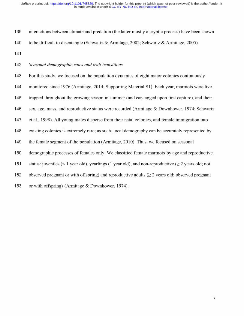
Figure 1: Seasonal life-cycle transitions modelled for yellow-bellied marmots. The two seasons correspond to the 155 main periods of mass loss (winter) and gain (summer). Solid and dashed arrows represent discrete-time stage 156 transitions and recruitment, respectively. Transitions among winter (W) and summer (S) stages (marked by arrows 157 in different colors) depend on demographic rates (survival [𝜃], reproduction [𝜑0], and recruitment [𝜑1]) and trait 158 transitions (mass change [𝛾], and offspring mass [𝜑2]). Stages are: juveniles, J, yearlings, Y, non-reproductive 159 adults, N, and reproductive adults, R. All stage-specific demographic rates and trait transitions are modeled using 160 generalized linear mixed effects models in a Bayesian framework and include body mass and a common latent 161 variable representing environmental quality as covariates. 162
163
We determined demographic rates (survival, reproduction, and recruitment) for two discrete 164
growing seasons: winter (August - June) and summer (June - August) (Fig. 1), delineating the 165
main periods of mass loss and gain, respectively (Maldonado-Chaparro et al., 2017). We 166
assumed that females that permanently disappeared from a colony had died. This measure of 167
apparent survival may overestimate the death of yearlings in the summer, which disperse from 168
their natal colonies (Van Vuren & Armitage, 1994). At the same time, the intensive trapping 169
protocol ensured a high capture probability of yearlings (Oli & Armitage, 2004), decreasing the 170
discrepancies between their apparent and true survival. 171
.CC-BY-NC-ND 4.0 International licenseis made available under aThe copyright holder for this preprint (which was not peer-reviewed) is the author/funder. It. https://doi.org/10.1101/745620doi: bioRxiv preprint
9
Female marmots give birth to one litter from mid-May to mid-June. In our population 172
model, females ≥ 2 year of age that survived the winter were considered reproductive adults at 173
the beginning of summer if they were observed to be pregnant or with pups, or non-reproductive 174
adults otherwise (Fig. 1). Upon successful reproduction, weaned offspring emerge from burrows 175
ca. 35 days after birth (Armitage et al., 1976); we therefore defined recruitment as the number of 176
female juveniles weaned by reproductive females that survive the summer (Fig. 1). The sex ratio 177
of female:male recruits was assumed to be 1:1 (Armitage & Downhower, 1974). Observations 178
and pedigree analyses allowed us to determine the mother of each new juvenile recruited into the 179
population (Ozgul et al., 2010). 180
To assess changes in body mass from one season to the next, we estimated body mass of 181
every female at the beginning of each season: June 1 (beginning of the summer season when 182
marmots begin foraging) and August 15 (beginning of the winter season in our models when 183
foraging activity decreases). Mid-August is the latest that body mass for the vast majority of 184
individuals can be measured and has been shown to be a good estimate of pre-hibernation mass 185
(Maldonado-Chaparro et al., 2017). Body-mass estimates on the two specific dates were 186
estimated using linear mixed effect models. These models were fitted for each age class and 187
included the fixed effect of day-of-year on body mass, and the random effects of year, site and 188
individual identity on the intercept and on the day-of-year slope (for details see Ozgul et al., 189
2010; Maldonado-Chaparro et al., 2017). Body mass of juvenile females was estimated for 190
August 15. 191
192
Modelling covariation in demographic processes – latent-variable approach 193
.CC-BY-NC-ND 4.0 International licenseis made available under aThe copyright holder for this preprint (which was not peer-reviewed) is the author/funder. It. https://doi.org/10.1101/745620doi: bioRxiv preprint
10
We jointly modeled all seasonal demographic and mass change rates (i.e., demographic 194
processes) as a function of stage and body mass - or mother’s mass in the case of juvenile mass - 195
at the beginning of a season, using a Bayesian modeling framework (Table 1; Supporting 196
Material S1). All mass estimates were cube-root transformed to stabilize the variance and 197
improve the normality of the residuals in the Gaussian submodels (Maldonado-Chaparro et al., 198
2017). We fitted all demographic-process submodels as generalized linear mixed effects models 199
(GLMMs). We assumed a binomial error distribution (logit link function) for the probability of 200
winter (𝜃W) and summer (𝜃S) survival and of probability of reproducing (i.e., being in the 201
reproductive adult stage at the beginning of summer; φ0); a Poisson error distribution (log link 202
function) for the number of recruits (φ1); and a Gaussian error distribution (identity link) for the 203
masses (z*) at the end of each season (Table 1). Mass-change (i.e., mass gain or loss) rates (𝛾) 204
were then defined as functions of current (z) and next (z*) mass using a normal probability 205
density function. For the juvenile mass distribution (φ2), the density function depended on the 206
mother’s mass (zM) (see below; Supporting Material S2). 207
To model temporal covariation in seasonal demography in the absence of explicit 208
knowledge on key biotic or abiotic drivers of this covariation, we used a factor-analytic 209
approach. This approach has recently been proposed by Hindle and coauthors (2018) as a 210
structured alternative to fit and project unstructured covariances among demographic processes 211
when factors explaining these covariances are not modeled. We implemented this novel 212
approach parameterizing a model-wide latent variable (Qy) which affected all demographic 213
processes in a given year (y) (for details see Supporting Material S1 and Hindle et al., 2018). Qy 214
was incorporated as a covariate in all seven demographic-process submodels (Table 1). Year-215
specific values of Qy were drawn from a normal distribution with mean = 0 and SD =1. The 216
.CC-BY-NC-ND 4.0 International licenseis made available under aThe copyright holder for this preprint (which was not peer-reviewed) is the author/funder. It. https://doi.org/10.1101/745620doi: bioRxiv preprint
11
associated βq slope parameters then determine the magnitude and sign of the effect of Qy on a 217
given, season-specific demographic process (Table 1). To make the Bayesian model identifiable, 218
we constrained the standard deviation of Qy to equal 1 and arbitrarily set the βq for summer 219
survival (𝜃S) to be positive. The βq of the remaining submodels can, therefore, be interpreted as 220
correlations of demographic processes with 𝜃S. 221
Aside from the latent variable Qy simultaneously affecting all demographic processes, we 222
included a random year effect (εYsubmodel) as a covariate in each submodel. While Qy captured 223
demographic covariation, the year effect accounted for additional temporal variation of each 224
demographic process not captured by Qy. We also tested for the effect of population density 225
(measured as total abundance, abundance of adults, or abundance of yearling and adults) in all 226
submodels. However, like previous studies, we could not detect any clear density effects 227
(Armitage, 1984; Maldonado-Chaparro et al., 2018). 228
The prior distributions of the Bayesian model and posterior parameter samples obtained 229
are detailed in Supporting Material S1. For each demographic-process submodel, we chose the 230
most parsimonious model structure by fitting a full model that included all covariates (mass, 231
stage, and Qy) and two-way interactions between mass and stage and stage and Qy, and retaining 232
only those parameters for which the posterior distribution (± 95 % C.I.) did not overlap 0 (Table 233
1; Table S1.1). 234
235
236
237
238
239
.CC-BY-NC-ND 4.0 International licenseis made available under aThe copyright holder for this preprint (which was not peer-reviewed) is the author/funder. It. https://doi.org/10.1101/745620doi: bioRxiv preprint
12
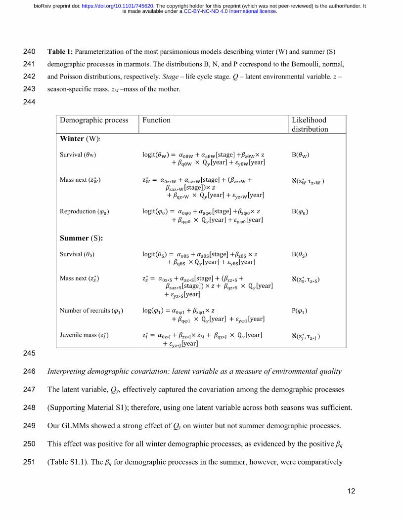
Table 1: Parameterization of the most parsimonious models describing winter (W) and summer (S) 240
demographic processes in marmots. The distributions B, N, and P correspond to the Bernoulli, normal, 241
and Poisson distributions, respectively. Stage – life cycle stage. Q – latent environmental variable. z – 242
season-specific mass. zM –mass of the mother. 243
244
245
Interpreting demographic covariation: latent variable as a measure of environmental quality 246
The latent variable, Qy, effectively captured the covariation among the demographic processes 247
(Supporting Material S1); therefore, using one latent variable across both seasons was sufficient. 248
Our GLMMs showed a strong effect of Qy on winter but not summer demographic processes. 249
This effect was positive for all winter demographic processes, as evidenced by the positive βq 250
(Table S1.1). The βq for demographic processes in the summer, however, were comparatively 251
Demographic process Function Likelihood distribution
Winter (W):
Survival (𝜃W) logit(𝜃+) = 𝛼01++𝛼31+[stage]+𝛽:1+×z+𝛽=1+ × Q?[year]+𝜀C1+[year]
B(𝜃+)
Mass next (𝑧E∗ )
zE∗ = 𝛼0:∗++𝛼3:∗+[stage]+(𝛽::∗+ +𝛽:3:∗+[stage])×𝑧
+𝛽=:∗+ × Q?[year]+𝜀C:∗+[year]
ℵ(zE∗ τ:∗+)
Reproduction (𝜑0) logit(𝜑0) = 𝛼0I0+𝛼3I0[stage]+𝛽:I0×z+𝛽=I0 × Q?[year]+𝜀CI0[year]
B(𝜑0)
Summer (S):
Survival (𝜃S) logit(𝜃J) = 𝛼01J+𝛼31J[stage]+𝛽:1J×𝑧+𝛽=1J × Q?[year]+𝜀C1J[year]
B(𝜃J)
Mass next (𝑧K∗) zK∗ = 𝛼0:∗J+𝛼3:∗J[stage]+(𝛽::∗J +𝛽:3:∗J[stage])×𝑧 +𝛽=:∗J ×Q?[year]+𝜀C:∗J[year]
ℵ(zK∗, τ:∗J)
Number of recruits (𝜑M)
log(𝜑M) =𝛼0IM+𝛽:IM×𝑧+𝛽=IM ×Q?[year]+𝜀CIM[year]
P(𝜑M)
Juvenile mass (𝑧N∗)
zN∗ =𝛼0:∗O+𝛽::∗O×𝑧P +𝛽=:∗O ×Q?[year]+𝜀C:∗O[year]
ℵ(zN∗, τ:∗O)
.CC-BY-NC-ND 4.0 International licenseis made available under aThe copyright holder for this preprint (which was not peer-reviewed) is the author/funder. It. https://doi.org/10.1101/745620doi: bioRxiv preprint
13
small and were not significantly different from 0 (95 % posterior C.I.s overlapped 0). The 252
positive βq indicate that Qy effectively estimates the overall annual environmental quality or 253
suitability, capturing both biotic and abiotic processes. A positive value of Qy then depicts an 254
environmental condition at a given time point that increases winter survival and probability of 255
reproducing and decreases mass loss (Hindle et al., 2018). The variation in Qy was in part 256
explained by environmental variables measured at the study site, but was unrelated to population 257
density (Supporting Material S1). Negative values of Qy were associated with longer and more 258
severe winters and a higher snow cover, while positive Qy indicated warmer winters and springs. 259
However, as the environmental variables explained < 50 % of the variation in Qy, the latent 260
variable captures multivariate, partly unobserved biotic and abiotic processes into a simple, 261
univariate measure of how bad (Qy < 0) or good (Qy > 0) environmental conditions are likely to 262
affect marmot demography. 263
Aside from the effects of environmental quality, our models are consistent with previous 264
findings on the importance of body mass and stage on yellow-bellied marmot demography 265
(Maldonado-Chaparro et al., 2017; Ozgul et al., 2010). The most parsimonious GLMMs (Table 266
S1.1) showed a positive effect of mass on all demographic processes, with the weakest effect of 267
mass on summer survival (𝜃S) of reproductive adults. Survival, in particular 𝜃S, was highest for 268
reproductive adults; reproduction was also highest for adults that reproduced before (Fig. S1.5). 269
270
Seasonal Integral Projection Models 271
We used the most parsimonious models of demographic processes (Table 1) to parameterize 272
density-independent, stage-mass-structured, seasonal and environment-specific Integral 273
Projection Models (IPMs) (Easterling et al., 2000; Ellner et al., 2016). For each stage a, the IPMs 274
.CC-BY-NC-ND 4.0 International licenseis made available under aThe copyright holder for this preprint (which was not peer-reviewed) is the author/funder. It. https://doi.org/10.1101/745620doi: bioRxiv preprint
14
track the number of individuals (na) in the mass range [z, z+dz] at time t. The fate of these 275
individuals at time t+1 is described by a set of coupled integral equations, which differ for each 276
season and are a function of the latent environmental variable Qy. In the winter season, 277
individuals can survive (𝜃w) and change mass (𝛾W) according to their stage, mass, and 278
environment. Conditional on survival, juveniles (J) transition to yearlings (Y), while all other 279
stages are distributed to either the reproductive (R) or non-reproductive (N) adult stage at the 280
beginning of summer, depending on the stage-specific probability of reproducing (φ0). During 281
the summer season, individuals in stages Y, N, and R survive (𝜃S) and change mass (𝛾S) 282
according to their stage and mass at the beginning of summer and according to the environment; 283
but, in summer, transitions to another stage do not occur. Reproductive individuals (R) of a given 284
mass also produce φ1/2 female juveniles (J), i.e., half of the total number of recruits. Female 285
recruits are distributed across z mass classes by the end of summer, given by φ2. The 286
mathematical descriptions of the IPMs for the winter and summer seasons are provided in 287
Supporting Material S2. Our population model assumes that past conditions affecting individuals 288
are captured by the current mass distribution and are propagated through time, allowing us to 289
assess trait- and stage-mediated demographic processes (Ozgul et al., 2010). 290
We numerically integrated the summer and winter IPMs using the ‘midpoint rule’ 291
(Easterling et al., 2000) with upper and lower integration limits of 7.8 (472 g) and 17.1 (5000 g), 292
respectively. To avoid unintended eviction of individuals from the model (i.e., for a given mass 293
class z, the sum of the probabilities to transition to z* < 1), we applied a constant correction (i.e., 294
equally redistributing evicted individuals among all z*) when constructing the IPMs as suggested 295
in Merow et al., (2014) (see also Williams et al., 2012). For each stage-specific IPM, we chose a 296
bin size of 100 (i.e., dividing masses into 100 classes), as further increasing the bin size did not 297
.CC-BY-NC-ND 4.0 International licenseis made available under aThe copyright holder for this preprint (which was not peer-reviewed) is the author/funder. It. https://doi.org/10.1101/745620doi: bioRxiv preprint
15
significantly improve the precision of estimates of the long-term population growth rate. The 298
IPMs we constructed accurately reproduced observed population dynamics from 1976-2016 299
(Supporting Material S2). 300
301
Sensitivity of population dynamics to seasonal demographic processes: prospective 302
perturbations 303
Changes in population dynamics in response to changes in environmental fluctuations are 304
determined by the response of demographic processes to the environment and, in turn, of 305
population dynamics to demographic processes (Maldonado-Chaparro et al., 2018). To explore 306
these two sources of variation in the long-term fitness of the marmot population, we first 307
quantified the proportional change in the demographic processes (Table 1) to changes in Qy, i.e., 308
𝜕(log ⍴)/𝜕Qy, where ⍴ is a demographic process. We calculated these elasticities for different 309
values of Qy (from -1 to 1), increasing each value by 0.01 and keeping mass at its stage-specific 310
average and εY fixed to 0. To assess the effect of parameter uncertainty on our estimates, we 311
repeated these calculations for a sample of 1000 parameter values drawn from the posterior 312
distribution (Paniw et al., 2017). 313
We next assessed which demographic processes most affected the stochastic population 314
fitness under observed (1976-2016) environmental fluctuations. We used a simulation of 100,000 315
years to assess the stochastic population growth rate, log 𝜆𝑠, a measure of fitness (see Supporting 316
Material S3 for details; see section below for short-term viability simulations). During the 317
simulation, we calculated the elasticity of log 𝜆𝑠 to changes in the 40-year observed mean (𝑒KV) 318
and standard deviation (𝑒KW) of stage-specific demographic processes; we adapted the approach 319
described in Ellner et al. (2016; chapter 7) to evaluate the relative effects of these changes on log 320
.CC-BY-NC-ND 4.0 International licenseis made available under aThe copyright holder for this preprint (which was not peer-reviewed) is the author/funder. It. https://doi.org/10.1101/745620doi: bioRxiv preprint
16
𝜆𝑠 (see S3 for details). The two elasticities quantify the strength of selection pressures on lower-321
level vital rates in stochastic environments (Haridas & Tuljapurkar, 2005; Rees & Ellner, 2009). 322
We repeated the elasticity calculations for a sample of 100 parameter values from the posterior 323
distribution. 324
Population viability under changes in environmental quality 325
To assess how the combined effects of (i) seasonal demographic responses to environmental 326
fluctuations and (ii) population sensitivity to seasonal demography impact population viability, 327
we simulated population dynamics under environmental change. We ran 200 independent 328
simulations each projecting population dynamics for 50 years. The projections were based on 329
several scenarios of changes in the distribution of environmental quality, Qy, corresponding to 330
changes in the average and standard deviation of winter length and harshness as well as 331
unobserved environmental drivers. We first created base simulations (i.e., no environmental 332
change) where Qy was picked from a normal distribution with 𝜇Q = 0 and σQ = 1 across all 333
demographic processes. This was appropriate, as we found no indication of temporal 334
autocorrelation in Qy (Supporting Material S1). Next, we approximated random future 335
fluctuations in Qy under different average environmental conditions. To do so, we sampled Qy 336
from a normal distribution fixing the average environmental quality (𝜇Q = -1, -0.5 , 0.5, 1) and its 337
variation (σQ = 0.6, 1.2) over the 50 years of projections. We then explored how a trend in 𝜇Q 338
would affect viability and mass distribution. To do so, we decreased the four 𝜇Q by 0.01 in each 339
year of the projections, keeping σQ unaltered. We also explored population-level effects of future 340
increases in the temporal autocorrelation in Qy as detailed in Supporting Material S4. All 341
simulations were repeated for a random sample of 1,000 parameters from the posterior 342
distribution to account for parameter uncertainty. 343
.CC-BY-NC-ND 4.0 International licenseis made available under aThe copyright holder for this preprint (which was not peer-reviewed) is the author/funder. It. https://doi.org/10.1101/745620doi: bioRxiv preprint

17
For all environmental-change scenarios, we recorded the probability of quasi-extinction 344
across the 200 simulations. Quasi-extinction was defined conservatively as the number of non-345
juvenile individuals (i.e., yearlings and non-reproductive and reproductive individuals) in the 346
population to be < 4, which corresponded to 10 % of their lowest observed number. 347
RESULTS 348
Sensitivity of population dynamics to seasonal demographic processes 349
In accordance with the posterior distribution of βq parameters, which did not cross 0 for winter 350
demographic processes, only winter demographic processes were significantly affected by small 351
changes in Qy (Fig. 2). Among the winter demographic processes, changes in Qy affected 352
reproduction across stages the most, followed by survival of juveniles (Fig. 2). 353
354
Figure 2: The sensitivity of seasonal demographic processes to environmental quality in marmots. Sensitivity is 355 assessed as proportional changes in demographic processes, ⍴, as environmental quality, Qy, increases slightly. This 356 sensitivity is measured with respect to different average values of Qy and across four different life-cycle stages: 357 juveniles (J), yearlings (Y), non-reproductive adults (N), and reproductive adults (R). The demographic processes 358 include winter (W; blue color tones) and summer (S; red color tones) survival (𝜃) and mass change (𝛾); and 359
N R
J Y
-1 -0.6 -0.2 0.2 0.6 1 -1 -0.6 -0.2 0.2 0.6 1
0.0000
0.0025
0.0050
0.0075
0.0100
0.0000
0.0025
0.0050
0.0075
0.0100
Qy
∂ (lo
g ρ
)/∂ Q
y
θS γS φ 1 φ 2
θW γW φ 0
.CC-BY-NC-ND 4.0 International licenseis made available under aThe copyright holder for this preprint (which was not peer-reviewed) is the author/funder. It. https://doi.org/10.1101/745620doi: bioRxiv preprint
18
probability of reproducing (φ0), recruitment (φ1), and juvenile mass (φ2). Points and error bars show averages ± 95 360 % C.I. across 1,000 posterior parameter samples obtained from the Bayesian population model. 361
362
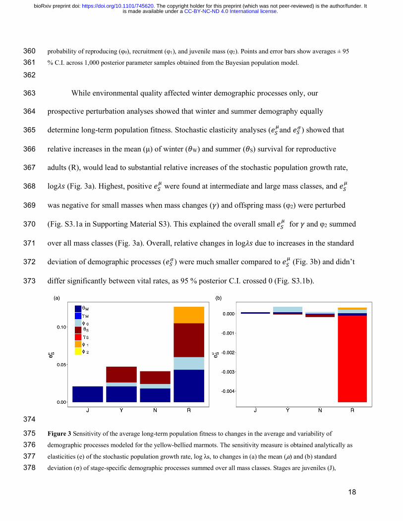
While environmental quality affected winter demographic processes only, our 363
prospective perturbation analyses showed that winter and summer demography equally 364
determine long-term population fitness. Stochastic elasticity analyses (𝑒KVand 𝑒KW) showed that 365
relative increases in the mean (µ) of winter (𝜃W) and summer (𝜃S) survival for reproductive 366
adults (R), would lead to substantial relative increases of the stochastic population growth rate, 367
log𝜆𝑠 (Fig. 3a). Highest, positive 𝑒KV were found at intermediate and large mass classes, and 𝑒K
V 368
was negative for small masses when mass changes (𝛾) and offspring mass (φ2) were perturbed 369
(Fig. S3.1a in Supporting Material S3). This explained the overall small 𝑒KV for 𝛾 and φ2 summed 370
over all mass classes (Fig. 3a). Overall, relative changes in log𝜆𝑠 due to increases in the standard 371
deviation of demographic processes (𝑒KW) were much smaller compared to 𝑒KV (Fig. 3b) and didn’t 372
differ significantly between vital rates, as 95 % posterior C.I. crossed 0 (Fig. S3.1b). 373
374
Figure 3 Sensitivity of the average long-term population fitness to changes in the average and variability of 375 demographic processes modeled for the yellow-bellied marmots. The sensitivity measure is obtained analytically as 376 elasticities (e) of the stochastic population growth rate, log λs, to changes in (a) the mean (𝜇) and (b) standard 377 deviation (σ) of stage-specific demographic processes summed over all mass classes. Stages are juveniles (J), 378
.CC-BY-NC-ND 4.0 International licenseis made available under aThe copyright holder for this preprint (which was not peer-reviewed) is the author/funder. It. https://doi.org/10.1101/745620doi: bioRxiv preprint
19
yearlings (Y), non-reproductive adults (N), and reproductive adults (R). Demographic processes include winter (W) 379 and summer (S) survival (𝜃) and mass change (𝛾); reproduction (φ0); recruitment (φ1), and offspring mass 380 distribution (φ2). Elasticities were calculated at the mean posterior values of parameters obtained from the Bayesian 381 demographic model. 382
383
Population viability under changes in environmental quality 384
While population fitness was equally sensitive to demographic processes over winter and 385
summer, environmental fluctuations strongly affected viability through winter demography. 386
Using base simulations (i.e., obtaining Qy from a normal distribution with 𝜇Q = 0 and σQ = 1), 387
the probability of quasi-extinction, at an average of 0.1 [0.0, 0.3 C.I.] across posterior 388
parameters, were relatively low. Simulations of population dynamics based on scenarios of 389
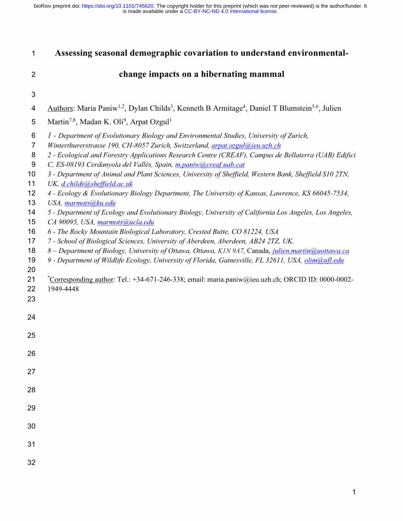
environmental change, corresponding in part to changes in winter length and harshness, resulted 390
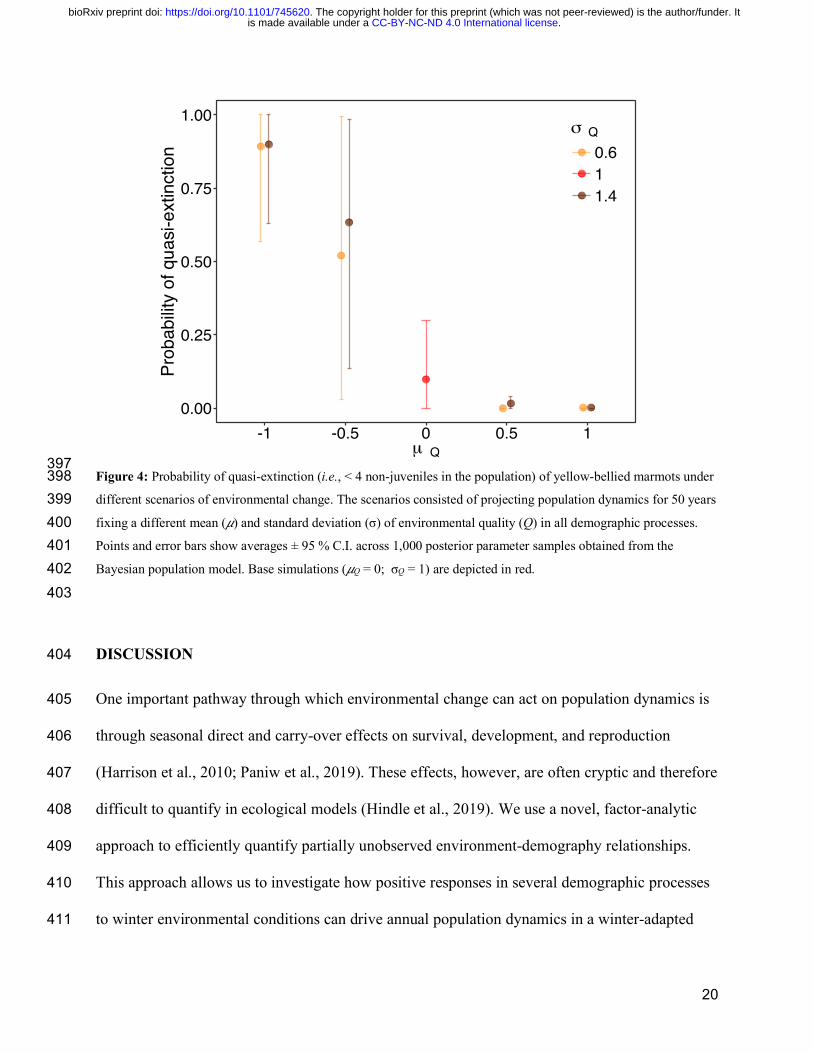
in substantial changes to viability. Quasi-extinction decreased (0 at 𝜇Q = 1) and increased (0.9 391
[0.6, 1.0 C.I.] at 𝜇Q = -1), compared to base simulations, when the population experienced a high 392
and low average environmental quality (Qy), respectively (Fig. 4). Average quasi-extinction 393
further increased and its uncertainty across posterior parameters decreased when a declining 394
trend in Qy was simulated (Fig. S4.1). Changes in the standard deviation (Fig. 4) and 395
autocorrelation (Fig. S4.2) of Qy had comparatively little effect on quasi-extinction. 396
.CC-BY-NC-ND 4.0 International licenseis made available under aThe copyright holder for this preprint (which was not peer-reviewed) is the author/funder. It. https://doi.org/10.1101/745620doi: bioRxiv preprint
20
397 Figure 4: Probability of quasi-extinction (i.e., < 4 non-juveniles in the population) of yellow-bellied marmots under 398 different scenarios of environmental change. The scenarios consisted of projecting population dynamics for 50 years 399 fixing a different mean (𝜇) and standard deviation (σ) of environmental quality (Q) in all demographic processes. 400 Points and error bars show averages ± 95 % C.I. across 1,000 posterior parameter samples obtained from the 401 Bayesian population model. Base simulations (𝜇Q = 0; σQ = 1) are depicted in red. 402 403
DISCUSSION 404
One important pathway through which environmental change can act on population dynamics is 405
through seasonal direct and carry-over effects on survival, development, and reproduction 406
(Harrison et al., 2010; Paniw et al., 2019). These effects, however, are often cryptic and therefore 407
difficult to quantify in ecological models (Hindle et al., 2019). We use a novel, factor-analytic 408
approach to efficiently quantify partially unobserved environment-demography relationships. 409
This approach allows us to investigate how positive responses in several demographic processes 410
to winter environmental conditions can drive annual population dynamics in a winter-adapted 411
0.00
0.25
0.50
0.75
1.00
-1 -0.5 0 0.5 1μ Q
Prob
abilit
y of
qua
si-e
xtin
ctio
n
σ Q0.611.4
.CC-BY-NC-ND 4.0 International licenseis made available under aThe copyright holder for this preprint (which was not peer-reviewed) is the author/funder. It. https://doi.org/10.1101/745620doi: bioRxiv preprint
21
mammal. The sensitivity to winter conditions occurs despite the fact that offspring are recruited 412
in summer and both summer and winter demographic processes determine population fitness. As 413
whole-year, population-level effects of environmental change can be filtered by season-specific 414
processes in the absence of density-dependent feedbacks, we highlight that the assessment of 415
such processes allows for a mechanistic understanding of population persistence (Picó et al., 416
2002; Paniw et al., 2019). 417
In marmots, as in numerous other populations (Bassar et al., 2016; Jenouvrier et al., 418
2018), seasonal demographic processes play an important role in life-cycle dynamics (Armitage, 419
2017). Our prospective perturbations show that changes in both mean winter and summer 420
survival of reproductive adults have the strongest effect on population fitness, confirming the 421
critical role of this life-cycle stage (Ozgul et al., 2009). At the same time, environmental 422
conditions do not affect adult survival or other demographic processes in the same way 423
throughout the year. That is, although the environment has been shown to drive particularly 424
recruitment in numerous temperate species (e.g., Bonardi et al., 2017; Nouvellet et al., 2013), 425
such effects are not evident in marmots; here, a higher annual environmental quality, which 426
increases all winter demographic processes, shows little impact on summer demography, 427
including recruitment. In turn, only these joint responses of winter demographic processes to 428
environmental quality determine population persistence under environmental change. 429
The complex, partially unmeasured environmental processes that cause positive 430
covariation in seasonal demographic processes can be effectively captured using a univariate, 431
latent measure of environmental quality. In our study, this latent quality correlated better with 432
observed annual population growth than any measured environmental variable (Supporting 433
Material S1). In part, a good quality depicts shorter and milder winters. Milder winters increase 434
.CC-BY-NC-ND 4.0 International licenseis made available under aThe copyright holder for this preprint (which was not peer-reviewed) is the author/funder. It. https://doi.org/10.1101/745620doi: bioRxiv preprint
22
food availability and the time available for vigilance, thereby decreasing predation risk (Van 435
Vuren, 2001), especially just before or after hibernation (i.e., within our winter season) when 436
such risk is severe (Armitage, 2014). Predation risk in early spring also increases under high 437
snow cover, as marmots, including more experienced adult females, cannot easily retreat to their 438
burrows (Blumstein, pers. obs.). Predation is however cryptic in the system (Van Vuren, 2001). 439
Capturing the effects of unobserved environmental variation, including predation, the latent-440
variable approach appears to be a promising alternative to modeling seasonal demographic 441
processes under limited knowledge of their drivers (Evans & Holsinger, 2012; Hindle et al., 442
2019; Hindle et al., 2018). We note that this approach may find limited applications in cases 443
where environment-demography relationships are more complex than in the yellow-bellied 444
marmots and include negative demographic covariation (e.g., due to opposing environmental 445
effects on demographic rates or tradeoffs between these rates). However, positive covariation in 446
demographic patterns is common (Jongejans et al., 2010; Paniw et al., 2019); and, given the short 447
time series of most demographic datasets (Salguero-Gómez et al., 2015; 2016) or little 448
knowledge on the actual environmental drivers of population dynamics (van de Pol et al., 2016; 449
Teller et al., 2016), the factor-analytic approach can be particularly useful in comparative 450
studies. 451
The seasonal effects of environmental quality on population persistence must be 452
understood in terms of the role of reproductive females in the marmot population (Ozgul et al., 453
2009). In our simulations, shorter and less sever winters (i.e., a good winter quality), would 454
result in more reproductive females in the summer (Armitage et al., 2003). In turn, summer 455
survival and recruitment by these females are important to long- and short-term demography 456
(Ozgul et al., 2009; Maldonado-Chaparro et al., 2018), but are not driven by environmental 457
.CC-BY-NC-ND 4.0 International licenseis made available under aThe copyright holder for this preprint (which was not peer-reviewed) is the author/funder. It. https://doi.org/10.1101/745620doi: bioRxiv preprint
23
conditions. That is, although predation affects individuals in summer (Van Vuren, 2001), its 458
effects are strongest on juveniles and yearlings, while adult females are little affected (Ozgul et 459
al., 2006). At the same time, as is the case in other socially complex mammals (Morris et al., 460
2011), reproduction in yellow-bellied marmots is governed primarily by social interactions, in 461
particular the behavior of dominant adult females (Armitage, 2010; Blumstein & Armitage, 462
1998). Even under optimal summer conditions, the reproductive output of the population may 463
not increase as dominant females suppress reproduction in younger subordinates and therefore 464
regulate the size of colonies (Armitage, 1991). Dominant females, in addition, may skip 465
reproduction themselves if they enter hibernation with a relatively low mass (Armitage, 2017). 466
Thus, the necessity of meeting the physiological requirements of hibernation profoundly affects 467
life-history traits of yellow-bellied marmots that are expressed during the active season. 468
Unlike the effects of seasonal survival and reproduction, trait transitions between seasons 469
had a smaller effect on annual population dynamics, even if winter mass changes were mediated 470
by environmental quality. These relatively small effects are likely due to the fact that marmots 471
compensate for winter mass loss with increased growth in the summer, creating a zero-net effect 472
on annual trait change (Maldonado-Chaparro et al., 2017; 2018). Although the strength of 473
compensatory effects may differ within seasons or among life-history stages (Monclús et al., 474
2014), such effects are common in rodents and other species that have a short window for mass 475
gain (Morgan & Metcalfe, 2001; Orizaola et al., 2014), and highlight how assessing seasonal 476
dynamics can provide a mechanistic understanding of population-level global-change effects 477
(Bassar et al., 2016). 478
Under environmental change, the persistence of marmots was mostly affected by changes 479
in mean environmental quality, whereas changes in the variance and temporal autocorrelation of 480
.CC-BY-NC-ND 4.0 International licenseis made available under aThe copyright holder for this preprint (which was not peer-reviewed) is the author/funder. It. https://doi.org/10.1101/745620doi: bioRxiv preprint
24
the mean showed little effects. This supports previous conclusions that yellow-bellied marmots 481
are partly buffered against increases in environmental variation (Maldonado-Chaparro et al., 482
2018; Morris et al., 2008) or autocorrelation (Engen et al., 2013). Further support for 483
demographic buffering comes from the fact that changes in the mean environmental quality most 484
strongly affected those demographic processes to which the stochastic population growth rate 485
was least sensitive, i.e., yearlings gaining reproductive status. It is well known that in species 486
where vital rates of adults are relatively buffered, juveniles are much more sensitive to 487
environmental variation (Gaillard & Yoccoz, 2003; Jenouvrier et al., 2018). Our results indicate 488
that demographic buffering (Pfister, 1998; Morris et al., 2008) likely persists across the seasonal 489
environments and different masses for a high-altitude specialist. 490
Our results emphasize that declines in environmental quality in the non-reproductive 491
season alone can strongly affect annual population dynamics of a mammal highly adapted to 492
seasonal environments. Therefore, positive demographic covariation under environmental 493
change may threaten populations even if it affects demographic process to which the stochastic 494
growth rate is least sensitive, i.e., processes that are under low selection pressure (Coulson et al., 495
2005; Iles et al., 2019). Studies that focus on the effects of environmental factors on single 496
demographic processes that strongly affect both short- and long-term population dynamics may 497
therefore underestimate the important role of seasonal demographic covariation. 498
Most species inhabit seasonal environments. Under global environmental change, it may 499
therefore be critical to understand how seasonal patterns mediate persistence of natural 500
populations. Novel methods such as the factor analytic approach allow researchers to overcome 501
some challenges associated with more mechanistic approaches assessing population responses to 502
.CC-BY-NC-ND 4.0 International licenseis made available under aThe copyright holder for this preprint (which was not peer-reviewed) is the author/funder. It. https://doi.org/10.1101/745620doi: bioRxiv preprint
25
environmental change, and we encourage more seasonal demographic analyses across different 503
taxa. 504
ACKNOWLEDGMENTS 505
We thank the many volunteers and researchers of Rocky Mountain Biological Laboratory for 506
collecting and providing us with the data on individual life histories of yellow-bellied marmots. 507
M.P. was supported by an ERC Starting Grant (33785) and a Swiss National Science Foundation 508
Grant (31003A_182286) to A.O.; and by a Spanish Ministry of Economy and Competitiveness 509
Juan de la Cierva-Formación grant FJCI-2017-32893; D.T.B. was supported by the National 510
Geographic Society (grant # 8140-06), the UCLA Faculty Senate and Division of Life Sciences, 511
a RMBL research fellowship, the National Science Foundation (IDBR-0754247, DEB-1119660 512
and 1557130 to D.T.B.; DBI 0242960, 0731346, and 1226713 to the RMBL). 513
REFERENCES 514
Armitage, K. B. (1984). Recruitment in yellow-bellied marmot populations: kinship, philopatry, 515
and individual variability. In J. O. Murie & G. R. Michener (Eds.), The Biology of Ground-516
Dwelling Squirrels (pp. 377–403), Lincoln: Univ. Nebraska Press. 517
Armitage, K. B. (1991). Social and population dynamics of yellow-bellied marmots: results from 518
long-term research. Annual Review of Ecology and Systematics, 22, 379–407. 519
Armitage, K. B. (2010). Individual fitness, social behavior, and population dynamics of yellow-520
bellied marmots. I. Billick & M.V. Price (Eds.) The Ecology of Place: Contributions of 521
Place-Based Research to Ecological Understanding (pp. 132–154), Chicago: University of 522
Chicago Press. 523
Armitage, K. B. (2014). Marmot Biology: Sociality, Individual Fitness, and Population 524
.CC-BY-NC-ND 4.0 International licenseis made available under aThe copyright holder for this preprint (which was not peer-reviewed) is the author/funder. It. https://doi.org/10.1101/745620doi: bioRxiv preprint
26
Dynamics. Cmbridge: Cambridge University Press. 525
Armitage, K. B. (2017). Hibernation as a major determinant of life-history traits in marmots. 526
Journal of Mammalogy, 98, 321–331. 527
Armitage, K. B., Blumstein, D. T., & Woods, B. C. (2003). Energetics of hibernating yellow-528
bellied marmots (Marmota flaviventris). Comparative Biochemistry and Physiology. Part A, 529
Molecular & Integrative Physiology, 134, 101–114. 530
Armitage, K. B., & Downhower, J. F. (1974). Demography of yellow-bellied marmot 531
populations. Ecology, 55, 1233–1245. 532
Armitage, K. B., Downhower, J. F., & Svendsen, G. E. (1976). Seasonal changes in weights of 533
marmots. The American Midland Naturalist, 96, 36–51. 534
Bassar, R. D., Letcher, B. H., Nislow, K. H., & Whiteley, A. R. (2016). Changes in seasonal 535
climate outpace compensatory density-dependence in eastern brook trout. Global Change 536
Biology, 22, 577–593. 537
Benton, T. G., Plaistow, S. J., & Coulson, T. N. (2006). Complex population dynamics and 538
complex causation: devils, details and demography. Proceedings. Biological Sciences, 273, 539
1173–1181. 540
Blumstein, D. T., & Armitage, K. B. (1998). Life history consequences of social complexity a 541
comparative study of ground-dwelling sciurids. Behavioral Ecology, 9, 8–19. 542
Bonardi, A., Corlatti, L., Bragalanti, N., & Pedrotti, L. (2017). The role of weather and density 543
dependence on population dynamics of Alpine-dwelling red deer. Integrative Zoology, 12, 544
61–76. 545
Bryant, A. A. & Page, R. W. (2005). Timing and causes of mortality in the endangered 546
Vancouver Island marmot (Marmota vancouverensis). Canadian Journal of Zoology, 83, 547
.CC-BY-NC-ND 4.0 International licenseis made available under aThe copyright holder for this preprint (which was not peer-reviewed) is the author/funder. It. https://doi.org/10.1101/745620doi: bioRxiv preprint
27
674–682. 548
Campos, F. A., Morris, W. F., Alberts, S. C., Altmann, J., Brockman, D. K., Cords, M., Pusey, 549
A., Stoinski, T. S., Strier, K. B., & Fedigan, L. M. (2017). Does climate variability influence 550
the demography of wild primates? Evidence from long-term life-history data in seven 551
species. Global Change Biology, 23, 4907–4921. 552
Childs, D. Z., Coulson, T. N., Pemberton, J. M., Clutton-Brock, T. H., & Rees, M. (2011). 553
Predicting trait values and measuring selection in complex life histories: reproductive 554
allocation decisions in Soay sheep. Ecology Letters, 14, 985–992. 555
Compagnoni, A., Bibian, A. J., Ochocki, B. M., Rogers, H. S., Schultz, E. L., Sneck, M. E., 556
Elderd, B. D., Iler, A. M., Inouye, D. W., Jacquemin, H., & Miller, T. E. X. (2016). The 557
effect of demographic correlations on the stochastic population dynamics of perennial 558
plants. Ecological Monographs, 86, 480–494. 559
Connell, S. D., & Ghedini, G. (2015). Resisting regime-shifts: the stabilising effect of 560
compensatory processes. Trends in Ecology & Evolution, 30, 513–515. 561
Coulson, T., Gaillard, J.-M., & Festa-Bianchet, M. (2005). Decomposing the variation in 562
population growth into contributions from multiple demographic rates. The Journal of 563
Animal Ecology, 74, 789–801. 564
Easterling, M. R., Ellner, S. P., & Dixon, P. M. (2000). Size-specific sensitivity: applying a new 565
structured population model. Ecology, 81, 694–708. 566
Ehrlén, J., & Morris, W. F. (2015). Predicting changes in the distribution and abundance of 567
species under environmental change. Ecology Letters, 18, 303–314. 568
Ehrlén, J., Morris, W. F., von Euler, T., & Dahlgren, J. P. (2016). Advancing environmentally 569
explicit structured population models of plants. The Journal of Ecology, 104, 292–305. 570
.CC-BY-NC-ND 4.0 International licenseis made available under aThe copyright holder for this preprint (which was not peer-reviewed) is the author/funder. It. https://doi.org/10.1101/745620doi: bioRxiv preprint
28
Ellner, S. P., Childs, D. Z., & Rees, M. (2016). Data-driven Modelling of Structured 571
Populations: A Practical Guide to the Integral Projection Model. Springer. 572
Engen, S., Sæther, B.-E., Armitage, K. B., Blumstein, D. T., Clutton-Brock, T. H., Dobson, F. S., 573
Festa-Bianchet, M., Oli, M. K., & Ozgul, A. (2013). Estimating the effect of temporally 574
autocorrelated environments on the demography of density-independent age-structured 575
populations. Methods in Ecology and Evolution, 4, 573–584. 576
Evans, M. E. K., & Holsinger, K. E. (2012). Estimating covariation between vital rates: a 577
simulation study of connected vs. separate generalized linear mixed models (GLMMs). 578
Theoretical Population Biology, 82, 299–306. 579
Gaillard, J.-M., & Yoccoz, N. G. (2003). Temporal variation in survival of mammals: A case of 580
environmental canalization? Ecology, 84, 3294–3306. 581
Gamelon, M., Grøtan, V., Nilsson, A. L. K., Engen, S., Hurrell, J. W., Jerstad, K., Phillips, A. S., 582
Røstad, O. W., Slagsvold, T., Walseng, B., Steneth, N. C., & Sæther, B.-E. (2017). 583
Interactions between demography and environmental effects are important determinants of 584
population dynamics. Science Advances, 3, e1602298. 585
Haridas, C. V., & Tuljapurkar, S. (2005). Elasticities in variable environments: properties and 586
implications. The American Naturalist, 166, 481–495. 587
Harrison, X. A., Blount, J. D., Inger, R., Norris, R. D., & Bearhop, S. (2010). Carry-over effects 588
as drivers of fitness differences in animals. The Journal of Animal Ecology, 80, 4–18. 589
Hindle, B. J., Pilkington, J. G., Pemberton, J. M., & Childs, D. Z. (2019). Cumulative weather 590
effects can impact across the whole life cycle. Global Change Biology, in press. 591
Hindle, B. J., Rees, M., Sheppard, A. W., Quintana-Ascencio, P. F., Menges, E. S., & Childs, D. 592
Z. (2018). Exploring population responses to environmental change when there is never 593
.CC-BY-NC-ND 4.0 International licenseis made available under aThe copyright holder for this preprint (which was not peer-reviewed) is the author/funder. It. https://doi.org/10.1101/745620doi: bioRxiv preprint
29
enough data: a factor analytic approach. Methods in Ecology and Evolution, 147, 115. 594
Iles, D. T., Rockwell, R. F., & Koons, D. N. (2019). Shifting vital rate correlations alter 595
predicted population responses to increasingly variable environments. The American 596
Naturalist, E57–E64. 597
Jenouvrier, S., Desprez, M., Fay, R., Barbraud, C., Weimerskirch, H., Delord, K., & Caswell, H. 598
(2018). Climate change and functional traits affect population dynamics of a long-lived 599
seabird. The Journal of Animal Ecology, 87, 906–920. 600
Jenouvrier, S., Holland, M., Stroeve, J., Barbraud, C., Weimerskirch, H., Serreze, M., & Caswell, 601
H. (2012). Effects of climate change on an emperor penguin population: analysis of coupled 602
demographic and climate models. Global Change Biology, 18, 2756–2770. 603
Jongejans, E., de Kroon, H., Tuljapurkar, S., & Shea, K. (2010). Plant populations track rather 604
than buffer climate fluctuations. Ecology Letters, 13, 736–743. 605
Knops, J. M. H., Koenig, W. D., & Carmen, W. J. (2007). Negative correlation does not imply a 606
tradeoff between growth and reproduction in California oaks. Proceedings of the National 607
Academy of Sciences of the United States of America, 104, 16982–16985. 608
Lawson, C. R., Vindenes, Y., Bailey, L., & van de Pol, M. (2015). Environmental variation and 609
population responses to global change. Ecology Letters, 18, 724–736. 610
Lenihan, C., & Vuren, D. V. (1996). Growth and survival of juvenile yellow-bellied marmots 611
(Marmota flaviventris). Canadian Journal of Zoology, 74, 297–302. 612
Maldonado-Chaparro, A. A., Blumstein, D. T., Armitage, K. B., & Childs, D. Z. (2018). 613
Transient LTRE analysis reveals the demographic and trait-mediated processes that buffer 614
population growth. Ecology Letters, 23, 1353. 615
Maldonado-Chaparro, A. A., Read, D. W., & Blumstein, D. T. (2017). Can individual variation 616
.CC-BY-NC-ND 4.0 International licenseis made available under aThe copyright holder for this preprint (which was not peer-reviewed) is the author/funder. It. https://doi.org/10.1101/745620doi: bioRxiv preprint
30
in phenotypic plasticity enhance population viability? Ecological Modelling, 352, 19–30. 617
Marra, P. P., Cohen, E. B., Loss, S. R., Rutter, J. E., & Tonra, C. M. (2015). A call for full 618
annual cycle research in animal ecology. Biology Letters, 11, 20150552. 619
Merow, C., Dahlgren, J. P., Metcalf, C. J. E., Childs, D. Z., Evans, M. E. K., Jongejans, E., 620
Record, S., Rees, M., Salguero-Gómez, R., & McMahon, S. M. (2014). Advancing 621
population ecology with integral projection models: a practical guide. Methods in Ecology 622
and Evolution, 5, 99–110. 623
Monclús, R., Pang, B., & Blumstein, D. T. (2014). Yellow-bellied marmots do not compensate 624
for a late start: the role of maternal allocation in shaping life-history trajectories. 625
Evolutionary Ecology, 28, 721–733. 626
Morgan, I. J., & Metcalfe, N. B. (2001). Deferred costs of compensatory growth after autumnal 627
food shortage in juvenile salmon. Proceedings. Biological Sciences, 268, 295–301. 628
Morris, W. F., Altmann, J., Brockman, D. K., Cords, M., Fedigan, L. M., Pusey, A. E., Stoinski, 629
T. S., Bronikowski, A. M., Alberts, S. C., & Strier, K. B. (2011). Low demographic 630
variability in wild primate populations: fitness impacts of variation, covariation, and serial 631
correlation in vital rates. The American Naturalist, 177, E14–E28. 632
Morris, W. F., Pfister, C. A., Tuljapurkar, S., Haridas, C. V., Boggs, C. L., Boyce, M. S., Bruna, 633
E. M., Church, D. R., Coulson, T., Doak, D. F., Forsyth, S., Gaillard, J.-M., Horvitz, C. C., 634
Kalisz, S., Kendall, B. E., Knight, T. M., Lee, C. T., & Menges, E. S. (2008). Longevity can 635
buffer plant and animal populations against changing climatic variability. Ecology, 89, 19–636
25. 637
Nouvellet, P., Newman, C., Buesching, C. D., & Macdonald, D. W. (2013). A multi-metric 638
approach to investigate the effects of weather conditions on the demographic of a terrestrial 639
.CC-BY-NC-ND 4.0 International licenseis made available under aThe copyright holder for this preprint (which was not peer-reviewed) is the author/funder. It. https://doi.org/10.1101/745620doi: bioRxiv preprint
31
mammal, the european badger (Meles meles). PloS One, 8, e68116. 640
Oli, M. K., & Armitage, K. B. (2004). Yellow-bellied marmot population dynamics: 641
demographic mechanisms of growth and decline. Ecology, 85, 2446–2455. 642
Orizaola, G., Dahl, E., & Laurila, A. (2014). Compensatory growth strategies are affected by the 643
strength of environmental time constraints in anuran larvae. Oecologia, 174, 131–137. 644
Ozgul, A., Childs, D. Z., Oli, M. K., Armitage, K. B., & Blumstein, D. T. (2010). Coupled 645
dynamics of body mass and population growth in response to environmental change. Nature, 646
466, 482-485. 647
Ozgul, A., Oli, M. K., & Armitage, K. B. (2009). Influence of local demography on asymptotic 648
and transient dynamics of a yellow-bellied marmot metapopulation. The American 649
Naturalist, 173, 517-530. 650
Ozgul, A., Oli, M. K., Olson, L. E., Blumstein, D. T., & Armitage, K. B. (2007). Spatiotemporal 651
variation in reproductive parameters of yellow-bellied marmots. Oecologia, 154, 95–106. 652
Paniw, M., Maag, N., Cozzi, G., Clutton-Brock, T., & Ozgul, A. (2019). Life history responses 653
of meerkats to seasonal changes in extreme environments. Science, 363, 631–635. 654
Paniw, M., Ozgul, A., & Salguero-Gómez, R. (2018). Interactive life-history traits predict 655
sensitivity of plants and animals to temporal autocorrelation. Ecology Letters, 21, 275–286. 656
Paniw, M., Quintana-Ascencio, P. F., Ojeda, F., & Salguero-Gómez, R. (2017). Accounting for 657
uncertainty in dormant life stages in stochastic demographic models. Oikos , 126, 900–909. 658
Pfister, C. A. (1998). Patterns of variance in stage-structured populations: evolutionary 659
predictions and ecological implications. Proceedings of the National Academy of Sciences of 660
the United States of America, 95, 213–218. 661
Picó, F. X., de Kroon, H., & Retana, J. (2002). An extended flowering and fruiting season has 662
.CC-BY-NC-ND 4.0 International licenseis made available under aThe copyright holder for this preprint (which was not peer-reviewed) is the author/funder. It. https://doi.org/10.1101/745620doi: bioRxiv preprint
32
few demographic effects in a Mediterranean perennial herb. Ecology, 83, 1991–2004. 663
Reed, T. E., Grøtan, V., Jenouvrier, S., Sæther, B.-E., & Visser, M. E. (2013). Population growth 664
in a wild bird is buffered against phenological mismatch. Science, 340, 488–491. 665
Rees, M., & Ellner, S. P. (2009). Integral projection models for populations in temporally 666
varying environments. Ecological Monographs, 79, 575–594. 667
Robert, A., Bolton, M., Jiguet, F., & Bried, J. (2015). The survival–reproduction association 668
becomes stronger when conditions are good. Proceedings. Biological Sciences, 282, 669
20151529. 670
Ruf, T., Bieber, C., Arnold, W., & Millesi, E. (2012). Living in a Seasonal World: 671
Thermoregulatory and Metabolic Adaptations. Springer Science & Business Media. 672
Rushing, C. S., Hostetler, J. A., Sillett, T. S., Marra, P. P., Rotenberg, J. A., & Ryder, T. B. 673
(2017). Spatial and temporal drivers of avian population dynamics across the annual cycle. 674
Ecology, 98, 2837–2850. 675
Salguero-Gómez, R., Jones, O. R., & Archer, C. R., et al. (2015). The COMPADRE Plant Matrix 676
Database: an open online repository for plant demography. Journal of Ecology, 103, 202-677
218. 678
Salguero-Gómez, R., Jones, O. R., Archer, C. R., et al. (2016). COMADRE: a global data base 679
of animal demography. The Journal of Animal Ecology, 85, 371–384. 680
Schwartz, O. A., & Armitage, K. B. (2002). Correlations between weather factors and life-681
history traits of yellow-bellied marmots. Proceedings of the 3rd International Marmot 682
Conference, Cheboksary, Russia. 683
Schwartz, O. A., & Armitage, K. B. (2005). Weather influences on demography of the yellow-684
bellied marmot (Marmota flaviventris). Journal of Zoology, 265, 73–79. 685
.CC-BY-NC-ND 4.0 International licenseis made available under aThe copyright holder for this preprint (which was not peer-reviewed) is the author/funder. It. https://doi.org/10.1101/745620doi: bioRxiv preprint
33
Schwartz, O. A., Armitage, K. B., & Van Vuren, D. (1998). A 32-year demography of yellow-686
bellied marmots (Marmota flaviventris). Journal of Zoology, 246, 337–346. 687
Teller, B. J., Adler, P. B., Edwards, C. B., Hooker, G., & Ellner, S. P. (2016). Linking 688
demography with drivers: climate and competition. Methods in Ecology and Evolution, 7, 689
171–183. 690
Töpper, J. P., Meineri, E., Olsen, S. L., Rydgren, K., Skarpaas, O., & Vandvik, V. (2018). The 691
devil is in the detail: non-additive and context-dependent plant population responses to 692
increasing temperature and precipitation. Global Change Biology, 24, 4657-4666. 693
Van de Pol, M., Bailey, L. D., McLean, N., Rijsdijk, L., Lawson, C. R., & Brouwer, L. (2016). 694
Identifying the best climatic predictors in ecology and evolution. Methods in Ecology and 695
Evolution, 7, 1246–1257. 696
Van de Pol, M., Vindenes, Y., Sæther, B.-E., Engen, S., Ens, B. J., Oosterbeek, K., & Tinbergen, 697
J. M. (2010). Effects of climate change and variability on population dynamics in a long-698
lived shorebird. Ecology, 91, 1192–1204. 699
Van Vuren, D. (2001). Predation on yellow-bellied marmots (Marmota flaviventris). The 700
American Midland Naturalist, 145, 94–100. 701
Van Vuren, D., & Armitage, K. B. (1994). Survival of dispersing and philopatric yellow-bellied 702
marmots: what is the cost of dispersal? Oikos, 69, 179–181. 703
Varpe, Ø. (2017). Life history adaptations to seasonality. Integrative and Comparative Biology, 704
57, 943–960. 705
Villellas, J., Doak, D. F., García, M. B., & Morris, W. F. (2015). Demographic compensation 706
among populations: what is it, how does it arise and what are its implications? Ecology 707
Letters, 18, 1139–1152. 708
.CC-BY-NC-ND 4.0 International licenseis made available under aThe copyright holder for this preprint (which was not peer-reviewed) is the author/funder. It. https://doi.org/10.1101/745620doi: bioRxiv preprint

34
Van Vuren, D., & Armitage, K. B. (1991). Duration of snow cover and its influence on life-709
history variation in yellow-bellied marmots. Canadian Journal of Zoology, 69, 1755–1758. 710
Williams, J. L., Miller, T. E. X., & Ellner, S. P. (2012). Avoiding unintentional eviction from 711
integral projection models. Ecology, 93, 2008–2014. 712
Woodroffe, R., Groom, R., & McNutt, J. W. (2017). Hot dogs: High ambient temperatures 713
impact reproductive success in a tropical carnivore. The Journal of Animal Ecology, 86, 714
1329–1338. 715
.CC-BY-NC-ND 4.0 International licenseis made available under aThe copyright holder for this preprint (which was not peer-reviewed) is the author/funder. It. https://doi.org/10.1101/745620doi: bioRxiv preprint
Recommended