Portland State University Portland State University
PDXScholar PDXScholar
Dissertations and Theses Dissertations and Theses
Spring 5-5-2014
Assessing Hydrologic and Water Quality Sensitivities Assessing Hydrologic and Water Quality Sensitivities
to Precipitation Changes, Urban Growth and Land to Precipitation Changes, Urban Growth and Land
Management Using SWAT Management Using SWAT
Alexander Michael Psaris Portland State University
Follow this and additional works at: https://pdxscholar.library.pdx.edu/open_access_etds
Part of the Water Resource Management Commons
Let us know how access to this document benefits you.
Recommended Citation Recommended Citation Psaris, Alexander Michael, "Assessing Hydrologic and Water Quality Sensitivities to Precipitation Changes, Urban Growth and Land Management Using SWAT" (2014). Dissertations and Theses. Paper 1783. https://doi.org/10.15760/etd.1782
This Thesis is brought to you for free and open access. It has been accepted for inclusion in Dissertations and Theses by an authorized administrator of PDXScholar. Please contact us if we can make this document more accessible: [email protected].
Assessing Hydrologic and Water Quality Sensitivities to Precipitation Changes, Urban
Growth and Land Management Using SWAT
by
Alexander Michael Psaris
A thesis submitted in partial fulfillment of the
requirements for the degree of
Master of Science
in
Geography
Thesis Committee:
Heejun Chang, Chair
Eugene Foster
Martin Lafrenz
Portland State University
2014

© 2014 Alexander Michael Psaris

i
Abstract
Precipitation changes and urban growth are two factors altering the state of water
quality. Changes in precipitation will alter the amount and timing of flows, and the
corresponding sediment and nutrient dynamics. Meanwhile, densification associated
with urban growth will create more impervious surfaces which will alter sediment and
nutrient loadings. Land and water managers often rely on models to develop possible
future scenarios and devise management responses to these projected changes. We use
the Soil and Water Assessment Tool (SWAT) to assess the sensitivities of stream flow,
sediment, and nutrient loads in two urbanizing watersheds in Northwest Oregon, USA to
various climate and urbanization scenarios. We evaluate the spatial patterns climate
change and urban growth will have on water, sediment and nutrient yields. We also
identify critical source areas (CSAs) and investigate how implementation of vegetative
filter strips (VFS) could ameliorate the effects of these changes. Our findings suggest
that: 1) Water yield is tightly coupled to precipitation. 2) Large increases in winter and
spring precipitation provide enough sub-surface storage to increase summertime water
yields despite a moderate decrease in summer precipitation. 3) Expansion of urban areas
increases surface runoff and has mixed effects on sediment and nutrients. 4)
Implementation of VFS reduces pollutant loads helping overall watershed health. This
research demonstrates the usefulness of SWAT in facilitating informed land and water
management decisions.

ii
Acknowledgements
This thesis would not have been possible without the help and support of my
family, friends, classmates, committee members and knowledgeable professionals. I’d
like to thank Heejun Chang for his guidance throughout these past three years. I’d also
like to thank Jim Almendinger who relentlessly offers advice to SWAT modelers
worldwide through the SWAT-User google group. I and many others have learned a
great deal about SWAT through his eloquent explanations. I’d like to thank Martin
Lafrenz for lending his expertise in the area of sediment and erosion processes. I’d like to
thank my lab mate and collaborator on the SESAME grant Wes Hoyer who is an
intelligent and pleasant person to work with. I’d like to thank Gene Foster for his
willingness to lend support and provide data from the DEQ. I’d like to thank Raj Kapour
from Clean Water Services for offering his expertise on the Tualatin River Basin, and
providing waste water treatment plant data. Finally, I’d like to thank the professors and
students of the Geography Department who have helped guide and support me
throughout my graduate career.
iii
Table of Contents
Acknowledgements ............................................................................................................. ii
List of Tables ...................................................................................................................... v
List of Figures .................................................................................................................... vi
1. Introduction .................................................................................................................... 1
2. Study Site ....................................................................................................................... 3
2.1 Tualatin ................................................................................................................... 3
2.2 Yamhill ................................................................................................................... 5
3. Data and Methods ........................................................................................................... 7
3.1 Data ......................................................................................................................... 7
3.2 SWAT Model .......................................................................................................... 8
3.3 Calibration and Validation .................................................................................... 10
3.5 Scenario Analysis.................................................................................................. 12
3.5.1 Climate Change ............................................................................................. 12
3.5.2 Urban Growth ............................................................................................... 13
3.5.3 Management .................................................................................................. 14
4. Results ........................................................................................................................... 16
4.1 Model Calibration ................................................................................................. 16
4.2 Future Changes Under Climate and Land Cover Change Scenarios ................... 18
4.2.1 Flow ............................................................................................................. 18
4.2.2 Sediment ...................................................................................................... 24
4.2.3 Total Nitrogen ............................................................................................... 26
4.2.4 Total Phosphorus .......................................................................................... 28
4.3 Location of CSAs ................................................................................................. 30
4.4 Management .......................................................................................................... 32
5. Discussion ..................................................................................................................... 34
5.1 Model Calibration ................................................................................................. 34

iv
5.2 Spatial Patterns of Flow, Sediment, and Nutrients ............................................... 35
5.3 Future Changes and Adaptive Management ........................................................ 38
6. Conclusions ................................................................................................................... 40
7. References Cited ........................................................................................................... 42
Appendix A: Model Configuration ................................................................................... 51
Appendix B: Sensitivity Analysis, Calibration, and Validation ....................................... 54
Appendix C: Uncertainty .................................................................................................. 60
Appendix D: Historic and Future Climate ........................................................................ 62
References Cited ............................................................................................................... 63

v
List of Tables
Table 1: SWAT model input data and their sources used in the current study ................... 7
Table 2: Gages used for model evaluation. F = Flow, TSS = Total Suspended Solids, TN
= Total Nitrogen, TP = Total Phosphorus. Calibration gages are italicized. ............. 12
Table 3: List of final calibrated parameters for Tualatin and Yamhill sub-basins. ......... 16
Table 4: Monthly calibration and validation results. ....................................................... 17
Table 5: Percent change in annual and seasonal precipitation and flow for Tualatin and
Yamhill under climate change and urban growth scenarios. ...................................... 22
Table 6: Percent change in annual and seasonal sediment loadings ................................ 25
Table 7: Percent change in annual and seasonal TN loadings. ........................................ 27
Table 8: Percent change in annual and seasonal TP loadings. ......................................... 29
Table 9: Comparison of top 5% sub-basins before and after VFS applied ...................... 33

vi
List of Figures
Figure 1: Map of the Tualatin and Yamhill River basins. Gage numbers are referenced
in Table 1. ..................................................................................................................... 4
Figure 2: Elevation, soils, land use, and precipitation datasets used in the SWAT model. 8
Figure 3: Area weighted changes in precipitation and temperature for each of the three
climate scenarios split by season (Winter=DJF, Summer=JJA). ................................ 13
Figure 4: Changes in precipitation, air temperature, and flow for the high urban scenario
for Tualatin: low (a), medium (b), and high (a) climate scenarios. Yamhill: low (d),
medium (e), high (f) climate scenarios. ...................................................................... 21
Figure 5: Percent change in average annual water yield by sub-basin. ........................... 23
Figure 6: Percent change in average summer water yield. .............................................. 24
Figure 7: Percent change in annual average sediment yields. ......................................... 26
Figure 8: Percent change in annual average TN yield. .................................................... 28
Figure 9: Percent change in annual average TP yields. ................................................... 30
Figure 10: Shifts in hotspots due to climate change and urbanization. ........................... 32
Figure 11: Spatial patterns of predicted flow, sediment, total nitrogen, and total
phosphorus. ................................................................................................................. 36

1
1. Introduction
Precipitation changes and urban growth are two major factors altering watershed
dynamics worldwide (Vorosmarty et al. 2000, Whitehead et al. 2009). Precipitation
drives the amount and timing of river flows (Chang et al. 2001; Choi 2008; Franzyk &
Chang 2009; Tu 2009; Praskievicz and Chang 2011), which in turn drive sediment and
nutrient loads (Randall and Mulla 2001; Tong and Chen 2002; Chang 2004; Tang et al
2005; Atasoy et al 2006). Urban growth increases impervious surface areas causing
flashier storm responses. The increased overland flows carry nutrients more rapidly to
streams and instream nutrient removal is negatively correlated to urbanization (Paul and
Meyer 2001; Meyer et al. 2005; Walsch et al. 2005).
Given these realities, land and water managers are interested in possible solutions
to ameliorate the negative changes to water quality. One such possibility is the addition
of vegetative filter strips. These are lands set aside to intercept runoff from crop lands,
range lands or other land uses before the water enters streams. These areas consist of
natural vegetation that filters sediment and nutrients from overland flows (Abu-Zreig
2001; Abu-Zreig et al. 2004). While this does not directly address urban pollutants, this
could serve to improve downstream water quality, helping improve overall watershed
health.
The Soil and Water Assessment Tool (SWAT) is a semi-distributed watershed
model developed by the USDA’s Agricultural Research Service to address the issue of

2
non-point source pollution (Arnold et al. 2011). It has the capacity to model large areas
with diverse land uses, and includes algorithms to test the effects of best management
techniques, including vegetative filter strips. Niraula et al (2013) used SWAT to identify
critical source areas of pollutants in their study basin. Gu and Sahu (2009) used SWAT
to locate high impact sub-basins and measure nutrient reductions after installing
filterstrips. Lam et al (2011) assess both the water quality as well as economic impacts of
installing filter strips. In this study we investigate the following research questions.
(1) How do water, sediment and nutrient yields change annually and seasonally
under precipitation changes and urban growth scenarios?
(2) What are the locations of CSAs and will these CSAs shift in the future under
the combined scenarios of climate change and urban development?
(3) What effect does implementation of VFS have on sediment and nutrient
yields?

3
2. Study Site
2.1 Tualatin
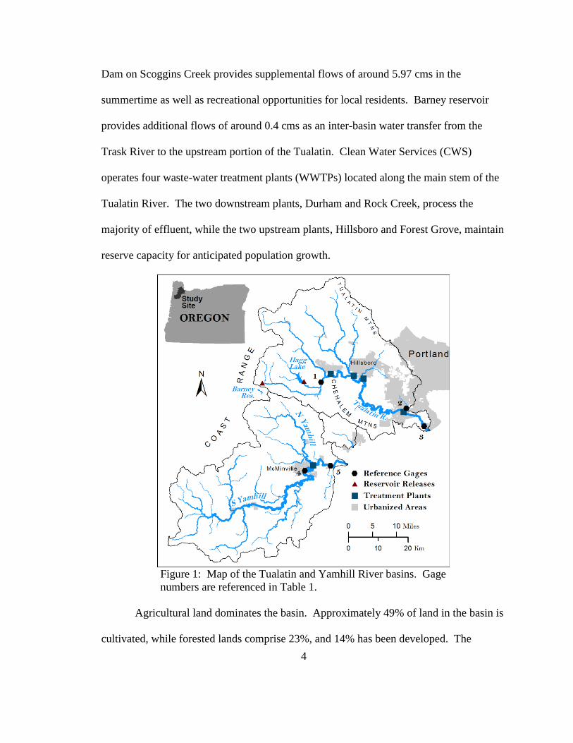
The 1,829 km2 Tualatin River Basin mostly shares the boundaries of Washington County
in Northwestern Oregon (Fig. 1). The basin is bordered by the Coast Range to the west,
Tualatin Mountains (West Hills) to the north and east, and the Chehalem Mountains to
the south. With the exception of its headwaters that originate in the Coast Range, the
Tualatin River is a low-gradient, meandering river that travels 130 km east, before
emptying into the Willamette River. Elevation in the basin ranges from a high of 1,057
m to a low of 17 m at the river’s mouth, and has a mean elevation of 195 m. Soils in the
basin formed from weathering of the Columbia River Basalts, and deposition of the
Willamette Silts by the Missoula Floods during the late Pleistocene. The region has a
modified marine climate, dominated by cool wet winters, and warm dry summers. In
upper elevations, annual precipitation ranges from 1,330 to 3,280 mm, and average daily
temperatures range from 4 to 27°C in the summer and -16 to 12°C in the winter. In the
valley, annual precipitation ranges from 740 to 1,850 mm, and average daily
temperatures range from 10 to 31°C in the summer, and -10 to 15°C in the winter
(Abazoglou 2013).
Stream flow is largely rain dominated with peak flows occurring throughout
January, and low flows occurring during July. The basin has a runoff ratio of 0.64 based
on 16 years of flow records. Two large dams alter the hydrology of the basin. Scoggins
4
Dam on Scoggins Creek provides supplemental flows of around 5.97 cms in the
summertime as well as recreational opportunities for local residents. Barney reservoir
provides additional flows of around 0.4 cms as an inter-basin water transfer from the
Trask River to the upstream portion of the Tualatin. Clean Water Services (CWS)
operates four waste-water treatment plants (WWTPs) located along the main stem of the
Tualatin River. The two downstream plants, Durham and Rock Creek, process the
majority of effluent, while the two upstream plants, Hillsboro and Forest Grove, maintain
reserve capacity for anticipated population growth.
Figure 1: Map of the Tualatin and Yamhill River basins. Gage
numbers are referenced in Table 1.
Agricultural land dominates the basin. Approximately 49% of land in the basin is
cultivated, while forested lands comprise 23%, and 14% has been developed. The
5
majority of the basin (93%) is privately owned. Of public lands, 5% is owned by the
State of Oregon and 2% is owned by the Bureau of Land Management (ODEQ 2001).
Due to agriculture, timber harvesting, and rapid urbanization in the mid-20th
century, the basin suffered from poor water quality. In 1988, EPA approved the first
TMDLs for temperature, bacteria, dissolved oxygen, pH, and phosphorus in the basin
(ODEQ 2001). Changes have been made to the TMDLs over the years as needs have
arisen, and water quality has improved. However, some rapidly urbanizing areas of the
basin still experience water quality problems (Boeder and Chang 2008; Pratt and Chang
2012). CWS is one of the designated management agencies in the basin, and is in charge
of monitoring and implementing their TMDL implementation plan. Climate change
studies in the region indicate that rising air temperatures will accentuate the seasonal
range of stream flows, with flows expected to increase in the winter and decrease in the
summer (Hamlet and Lettenmaier 1999; Franczyk and Chang 2009; Chang and Jung
2010; Praskievicz and Chang 2011).
2.2 Yamhill
The Yamhill sub-basin lies to the south of the Tualatin, and drains 1,998 km2
(Figure 1). The two main rivers, North and South Yamhill, flow southeast and northeast,
respectively, until they converge and flow east before emptying into the Willamette
River. Elevation in the basin ranges from 1,084 m in the Coast Range to 18 m at the
mouth of the Yamhill and has a mean elevation of 217 m. Soils in the basin have similar
6
provenance to those in the Tualatin. Annual precipitation ranges from 1,560 to 3,880 mm
in high elevations and 560 to 1,710 mm in lower elevations. Average daily temperatures
at high elevations range from -14 to 12 degrees in the winter and 7 to 27 degrees in the
summer. Low elevation daily temperatures range from -10 to 15 degrees in the winter
and 10 to 30 degrees in the summer.
The Yamhill River system is much less managed than the Tualatin. There is no
major reservoir in the Yamhill to supplement flows or provide flood control; hence,
during summer measured flows have dropped to as little as 0.04 cms, while winter wet
seasons have had flows as large as 1141 cms. The runoff ratio is 0.55. 40% of the basin
is forested. One third of the basin consists of cultivated crops. 10% of the basin consists
of shrubland, and only 7% is developed.
7
3. Data and Methods
3.1 Data
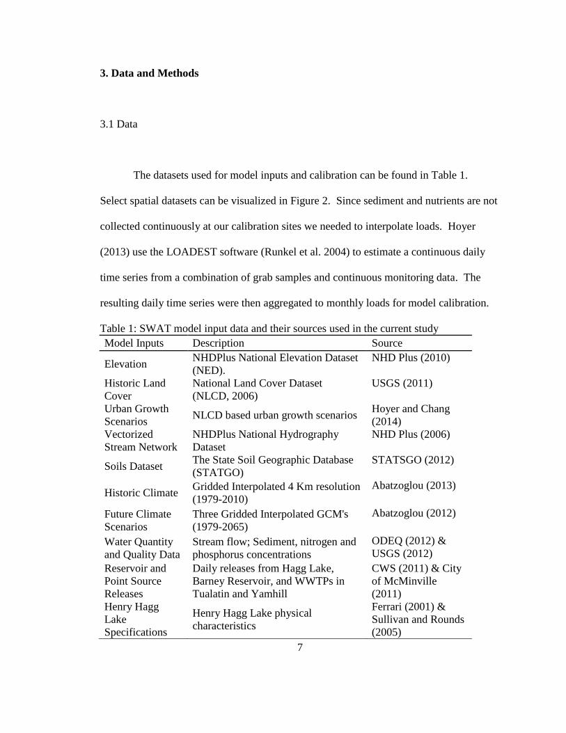
The datasets used for model inputs and calibration can be found in Table 1.
Select spatial datasets can be visualized in Figure 2. Since sediment and nutrients are not
collected continuously at our calibration sites we needed to interpolate loads. Hoyer
(2013) use the LOADEST software (Runkel et al. 2004) to estimate a continuous daily
time series from a combination of grab samples and continuous monitoring data. The
resulting daily time series were then aggregated to monthly loads for model calibration.
Table 1: SWAT model input data and their sources used in the current study
Model Inputs Description Source
Elevation NHDPlus National Elevation Dataset
(NED).
NHD Plus (2010)
Historic Land
Cover
National Land Cover Dataset
(NLCD, 2006)
USGS (2011)
Urban Growth
Scenarios NLCD based urban growth scenarios
Hoyer and Chang
(2014)
Vectorized
Stream Network
NHDPlus National Hydrography
Dataset
NHD Plus (2006)
Soils Dataset The State Soil Geographic Database
(STATGO)
STATSGO (2012)
Historic Climate Gridded Interpolated 4 Km resolution
(1979-2010)
Abatzoglou (2013)
Future Climate
Scenarios
Three Gridded Interpolated GCM's
(1979-2065)
Abatzoglou (2012)
Water Quantity
and Quality Data
Stream flow; Sediment, nitrogen and
phosphorus concentrations
ODEQ (2012) &
USGS (2012)
Reservoir and
Point Source
Releases
Daily releases from Hagg Lake,
Barney Reservoir, and WWTPs in
Tualatin and Yamhill
CWS (2011) & City
of McMinville
(2011)
Henry Hagg
Lake
Specifications
Henry Hagg Lake physical
characteristics
Ferrari (2001) &
Sullivan and Rounds
(2005)

8
Figure 2: Elevation, soils, land use, and precipitation datasets used in
the SWAT model.
3.2 SWAT Model
SWAT is a physically based, semi-distributed daily time-step model (SWAT 2012
rev. 613; Arnold et al 1998). It accounts for both terrestrial and in-stream processes. To
model flow, SWAT uses the Soil Conservation Service (SCS) curve number approach
(SCS 1972). To model sediment transport across the landscape, SWAT uses the
Modified Universal Soil Loss Equation (MUSLE, Williams 1975), an event scale variant
of the USLE that uses surface runoff instead of precipitation as a measure of erosive

9
energy. The nitrogen mass balance is budgeted into five pools and two main categories.
Mineral N consists of the ammonia and nitrate pools, while organic N consists of the
fresh organic N (biomass) and active and stable organic N pools. The Phosphorus mass
balance is budgeted into six pools split between mineral and organic P. Mineral P
consists of the stable, active, and solution pools, while organic P consists of the stable,
active, and fresh (biomass) pools (Neitsch et al. 2011). Channel sediment deposition and
re-entrainment are modeled using the Simplified Bangold equation. SWAT models in-
stream nutrient processes with algorithms from the QUAL2E model (Brown and
Barnwell 1987).
SWAT models watershed processes at three spatial scales. The first is the
watershed. This is essentially the final model output at the mouth of the river. The
second meso-scale of analysis is the sub-basin. These are stream reaches and their
contributing areas. Users can add additional sub-basins so that a sub-basin’s downstream
edge corresponds with calibration gages or other important watershed characteristics such
as point source inputs. Finally, the most basic unit of analysis in SWAT is the hydrologic
response unit (HRU). Each sub-basin has a unique set of HRUs which consist of pixels
with similar soil, slope, and land use characteristics. HRUs are aspatial, which means
that pixels do not need to be contiguous in order to be grouped together into one HRU.
Each HRU can be conceptualized as a field with constant slope, bordering the stream
reach. SWAT calculates the flow, sediment and nutrient yields from an HRU, adds it to
what was delivered from the upstream reach, and then calculates in-stream processes.
Therefore, all yields are assumed to enter the stream at the upper most boundary of its
10
sub-basin. This conceptualization enables SWAT to aggregate detailed field level
processes and management activities up to the watershed scale (Neitch et al 2011). For
example, filter strips and many other best management practices are modeled at the HRU
scale. However, the drawback is that the model is not fully distributed and certain spatial
processes such as explicit routing of lateral flow between HRUs and unique flow paths to
the stream reach are lost.
3.3 Calibration and Validation
We chose to perform manual calibration so that interactions between parameters
could be captured and multiple calibration objectives could be considered at once. We
performed a sensitivity analysis to help inform our parameter selection. We then adjusted
the most sensitive parameters to acquire a good fit. We calibrated flow first since it
drives sediment and nutrient loads. Since nutrients often travel to the stream bound to
sediment we calibrated sediment second and nitrogen and phosphorous last. We used one
gage to calibrate the Tualatin, and two additional gages to assess spatial accuracy of
Tualatin’s calibrated model. We used the USGS Dilley gage (Gage #1 in Figure 1 and
Table 2) for calibration since it is unaffected by the four downstream WWTPs. We used
one gage and one monitoring station to calibrate the Yamhill. We used the USGS gage in
McMinville (Gage # 4 in Figure 1 and Table 2) to calibrate flow, and a DEQ station
(Gage # 5 in Figure 1 and Table 2) to calibrate sediment and nutrients.
11
We measured the efficacy of the model with three metrics suggested by Moriasi
(2007): Nashe-Sutcliffe Efficiency (NSE), percent bias (PBIAS), and the RMSE-
observations standard deviation (RSR).
The NSE is calculated as
∑
∑
(1)
where represents the number of observations, is the observed data point,
is the simulated data point, and is the mean of all the observed data points. If
the model perfectly fits the observed data, . If the model is just as good as
taking the mean of the observed data, . If the mean of the observed data is a
better representation than the model, . We aimed to achieve an NSE score of at
least 0.5 (Moriasi 2007).
PBIAS is a measure of the model’s tendency to either over or under-predict, and
is calculated as
∑ (
)
∑
(2)
If the model on average over predicts, PBIAS is greater than 0. Under-predictions result
in a negative PBIAS. According to Moriasi (2007) PBIAS should be less than 25% for
flow, less than 55% for sediment, and less than 70% for nutrients. Using the parameters
we chose based off of our sensitivity analysis and the recommended goals outlined by
Moriasi (2007), reproducing this calibration should be possible. To acquire exactly the
same results it would most likely be better to use a deterministic automatic calibration
routine. However, given the computational requirements of automatic calibration, and
12
the fact that we did not have a calibration program available to us which could use the
three objective functions we chose, we felt the best method to consider all three metrics
simultaneously was manual calibration.
The third metric is designed to give a description of the model’s absolute error,
and is calculated as
√∑
√∑
(3)
Where is the root mean square error, and is the standard deviation of
the observed data. Moriasi (2007) recommends that for all constituents.
Table 2: Gages used for model evaluation. F = Flow, TSS = Total Suspended Solids, TN
= Total Nitrogen, TP = Total Phosphorus.
Gage # Name Organization ID # Constituents
1 Tualatin River at Dilley USGS/CWS 14203500 F, TSS, TN, TP
2 Fanno Creek at Durham USGS/CWS 14206950 F, TSS, TN, TP
3 Tualatin River at West
Linn USGS/CWS 14207500 F, TSS, TN, TP
4 South Yamhill River at
McMinnville USGS 14194150 F
5 Yamhill Water Quality
Station DEQ 10363 S, TN, TP
3.5 Scenario Analysis
3.5.1 Climate Change
Three downscaled global climate models with future scenarios for the time period
1981-2065 were selected in order to cover a range of possible realities. The GFDL-
ESM2M (“low”) scenario (MACA 2013) has a 0.08 °C change in average annual

13
temperature, and a 4.47% increase in average annual precipitation. The MIROC5
(“medium”) scenario (MACA 2013) has a 0.87 °C increase in average annual temperature
and a 12.75% increase in average annual precipitation. The HadGEM2-ES (“high”)
scenario (MACA 2013) has a 1.38 °C increase in annual average temperature and a
0.44% decrease in average annual precipitation. Seasonal changes for the scenarios can
be seen in Figure 3. The low scenario sees precipitation increase in both winter and
summer seasons. Precipitation increases during the winter and decreases substantially
during the summer in the medium scenario. Finally, precipitation remains roughly the
same during the winter, but decreases substantially during the summer in the high
scenario.
Figure 3: Area weighted changes in precipitation and temperature for
each of the three climate scenarios split by season (Winter=DJF,
Summer=JJA).
3.5.2 Urban Growth
14
Hoyer and Chang (2014), with relevant stakeholder consultation, developed land
cover change scenarios reflecting possible expansion of urban areas centered on the year
2050. The relative growth of urban areas was based on historical growth rates and
projected increases in annual population in the study area. The low scenario assumes an
annual growth rate of 0.6% and the high scenario assumes a 2.0% annual growth rate.
Land conversion is based on a graded weight matrix comprised of six factors: urban
growth boundary (UGB), distance from the UGB, zoning, groundwater restriction zones,
high value farm soils, and measure 49 claims which provide exemptions to landowners
who purchased land inside the urban growth boundary (UGB) before the UGB
regulations were instituted. A spatial mask was used to exclude urban growth from
protected lands.
3.5.3 Management
We apply the Vegetative Filter Strip model in SWAT for two representative years
in the study period (WY 1994 and 1995). The model was developed from the Vegetative
Filter Strip MODel (VFSMOD, Munoz-Capena, 1999), and designed to apply to HRUs in
SWAT. The algorithm permits a percentage of overland flow to be filtered before it
leaves an HRU and enters the stream reach. When overland flow encounters vegetation it
slows and its sediment carrying capacity becomes reduced. It also provides extra time for
runoff to infiltrate the soil and deposit sediment along with it.

15
For the sake of simplicity, the VFS model in SWAT assumes that the amount of
TN and TP filtered out of overland flow is related to sediment reduction. This is
assumption is backed up by studies demonstrating that the bulk of nitrogen and
phosphorus travel in particulate form off of agricultural fields (White and Arnold 2009).
We apply the VFS model to 5 sub-basins that exhibit the top 5% sediment and
nutrient loads based on a weighted index over the 30 year historic period. The weighted
index is comprised of sediment, TN, and TP yields using the following formula:
(4)
is the index value, S is the sediment yield (tons/ha), is the TN yield (kg/ha), and is
the TP yield (kg/ha). We gave sediment the highest weight since in high concentrations it
is considered a pollutant and it transports both nitrogen and phosphorus, two nutrients
commonly found to exceed natural concentrations as a result of agricultural activities and
urban development (ODEQ 2001).

16
4. Results
4.1 Model Calibration
Table 3 reports a summary of the twelve fitted parameter values. Due to a lack of
empirical data on channel erodibility, and sediment sources and sinks, we calibrated
sediment using MUSLE parameters only. Uncertainties in measured data, LOADEST
estimates, and temporal non-stationarity in flow, sediment and nutrient loadings, mean
that these values represent estimates of true parameter values only. Metrics were all in
acceptable ranges according to Moriasi et al. (2007) during calibration. RSR values for
TN and TP at the DEQ station were slightly higher than the recommended value of 0.7
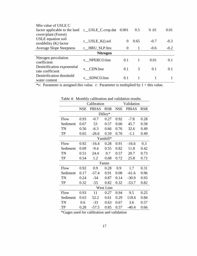
during validation, but all other metrics had acceptable values. Table 4 shows a summary
of monthly model fit metrics.
Table 3: List of final calibrated parameters for Tualatin and Yamhill sub-basins.
Description Parameter Min Max Tualatin
Value
Yamhill
Value
Flow
Baseflow alpha factor
(days) v__ALPHA_BF.gw* 0 1 1 1
Soil evaporation
compensation factor v__ESCO.bsn 0.01 1 1 0
Plant uptake compensation
factor v__EPCO.bsn 0 1 0.01 1
Available water capacity of
the soil layer r__SOL_AWC().sol -0.2 0.2 -0.2 -0.2
Threshold depth of water in
the shallow aquifer required
for return flow to occur
(mm)
v__GWQMN.gw 0 5000 0.1 0.1
Sediment
Average slope length r__SLSUBBSN.hru 10 150 -0.7 -0.4
17
Min value of USLE C
factor applicable to the land
cover/plant (Forest)
r__USLE_C.crop.dat 0.001 0.5 0 .01 0.01
USLE equation soil
erodibility (K) factor r__USLE_K().sol 0 0.65 -0.7 -0.3
Average Slope Steepness r__HRU_SLP.hru 0 1 -0.6 -0.2
Nitrogen
Nitrogen percolation
coefficient v__NPERCO.bsn 0.1 1 0.01 0.1
Denitrification exponential
rate coefficient v__CDN.bsn 0.1 3 0.1 0.1
Denitrification threshold
water content v__SDNCO.bsn 0.1 1 1 1
*v: Parameter is assigned this value. r: Parameter is multiplied by 1 + this value.
Table 4: Monthly calibration and validation results.
Calibration Validation
NSE PBIAS RSR NSE PBIAS RSR
Dilley*
Flow 0.93 -0.7 0.27 0.92 -7.8 0.28
Sediment 0.67 53 0.57 0.66 45.7 0.58
TN 0.56 -6.3 0.66 0.76 32.6 0.49
TP 0.65 -26.6 0.59 0.76 -1.1 0.49
Yamhill*
Flow 0.92 -16.4 0.28 0.91 -16.6 0.3
Sediment 0.69 -9.4 0.55 0.82 11.8 0.42
TN 0.51 24.4 0.7 0.57 20.7 0.73
TP 0.54 1.2 0.68 0.72 25.8 0.72
Fanno
Flow 0.92 0.9 0.28 0.9 1.7 0.31
Sediment 0.17 -57.4 0.91 0.08 -61.6 0.96
TN 0.24 -34 0.87 0.14 -30.9 0.93
TP 0.32 -55 0.82 0.32 -53.7 0.82
West Linn
Flow 0.93 11 0.27 0.94 9.5 0.25
Sediment 0.63 52.2 0.61 0.29 118.6 0.84
TN 0.6 -33 0.63 0.67 3.6 0.57
TP 0.28 -57.5 0.85 0.57 -40.4 0.66
*Gages used for calibration and validation
18
4.2 Future Changes Under Climate and Land Cover Change Scenarios
4.2.1 Flow
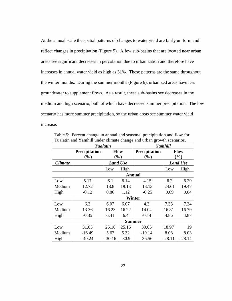
Average annual basin-wide flows increase in all scenarios due to the combination
of urbanization and increased precipitation. While there is a slight decrease in annual
precipitation in the high climate scenario, impervious surfaces decrease infiltration and
contribute to a slight increase in annual water yield (Table 5).
Changes in wintertime flows follow the same pattern as annual flows since a
significant portion of precipitation falls during winter months. In all scenarios wintertime
flow increases by a greater percentage than precipitation due to increased impervious
surfaces. Fall is the only season where precipitation increases in the high climate
scenario (Figure 4). The slight lag between precipitation and runoff means that flows still
increase during the winter despite a slight decrease in rain in winter. The lag between
runoff and precipitation can be seen clearly in all scenarios. Peak flows typically occur a
month or two after precipitation (Figure 4).
Summertime flows have a mixed response. In the low climate scenario flows
increase by a smaller percentage than precipitation due to increased evapotransporation.
In the medium climate scenario, summer-time flows contain a large baseflow component
due to large winter and spring rains (Figure 4). These groundwater inputs enable
summer-time flows to increase despite a decrease in summer precipitation greater than

19
15%. Under the high scenario, summer-time flow decreases by a smaller percentage than
precipitation due to more evapotranspiration.

20
(a)
(b)
(c)

21
Figure 4: Changes in precipitation, air temperature, and flow for the
high urban scenario for Tualatin: low (a), medium (b), and high (a)
climate scenarios. Yamhill: low (d), medium (e), high (f) climate
scenarios.
(d)
(e)
(f)
22
At the annual scale the spatial patterns of changes to water yield are fairly uniform and
reflect changes in precipitation (Figure 5). A few sub-basins that are located near urban
areas see significant decreases in percolation due to urbanization and therefore have
increases in annual water yield as high as 31%. These patterns are the same throughout
the winter months. During the summer months (Figure 6), urbanized areas have less
groundwater to supplement flows. As a result, these sub-basins see decreases in the
medium and high scenario, both of which have decreased summer precipitation. The low
scenario has more summer precipitation, so the urban areas see summer water yield
increase.
Table 5: Percent change in annual and seasonal precipitation and flow for
Tualatin and Yamhill under climate change and urban growth scenarios.
Tualatin Yamhill
Precipitation
(%)
Flow
(%)
Precipitation
(%)
Flow
(%)
Climate
Land Use
Land Use
Low High
Low High
Annual
Low 5.17 6.1 6.14 4.15 6.2 6.29
Medium 12.72 18.8 19.13 13.13 24.61 19.47
High -0.12 0.86 1.12 -0.25 0.69 0.04
Winter
Low 6.3 6.07 6.07 4.3 7.33 7.34
Medium 13.36 16.23 16.22 14.04 16.81 16.79
High -0.35 6.41 6.4 -0.14 4.86 4.87
Summer
Low 31.85 25.16 25.16 30.05 18.97 19
Medium -16.49 5.67 5.32 -19.14 8.08 8.03
High -40.24 -30.16 -30.9 -36.56 -28.11 -28.14

23
Figure 5: Percent change in average annual water yield by sub-basin.

24
Figure 6: Percent change in average summer water yield.
4.2.2 Sediment
There are basin-wide decreases in sediment in Tualatin under the low climate
scenario annually and during the winter despite increases in impervious surfaces (Table
6). Erosion increases during the summer due to a 31.8% increase in precipitation.
Yamhill sees uniform increases in sediment under the low climate scenario due to less

25
urban growth which permits moderate increases in precipitation to increase erosion. Both
basins see increases in sediment during the medium scenario, reflecting the universal
increase in precipitation and flows for the basin. While Tualatin sees sediment increase
under the high climate scenario both annually and during the winter, Yamhill has a
decrease annually and a slight increase during the winter. Some of the shifts in sediment
seem counter intuitive when compared to the precipitation changes.
Table 6: Percent change in annual and
seasonal sediment loadings
Tualatin Yamhill
Climate Land Use
Low High Low High
Annual
Low -7.6 -7.64 6.5 6.77
Medium 38.5 48.17 29.6 22.19
High 17.58 27.69 -2.84 -2.63
Winter
Low -11.95 -11.95 6.88 7.26
Medium 33.85 42.29 16.22 16.63
High 24.27 33.9 1.75 2.03
Summer
Low 81.96 82 73.06 73.04
Medium 6.82 13.38 5.62 5.42
High -44.37 -42.45 -38.91 -39
The spatial patterns of sediment yields suggest areas of high slope exhibit the
highest sediment yields (near the basin boundaries), reflecting the important role slope
plays in erosional processes (Figure 7). Cultivated agricultural lands are located on fairly
flat terrain, and therefore do not exhibit erosion rates as high as those for hay and
rangeland which are located on a mix of flat and high sloping areas. Changes in erosion
resulting from climate change respond in unpredictable ways. Forest, hay and range lands
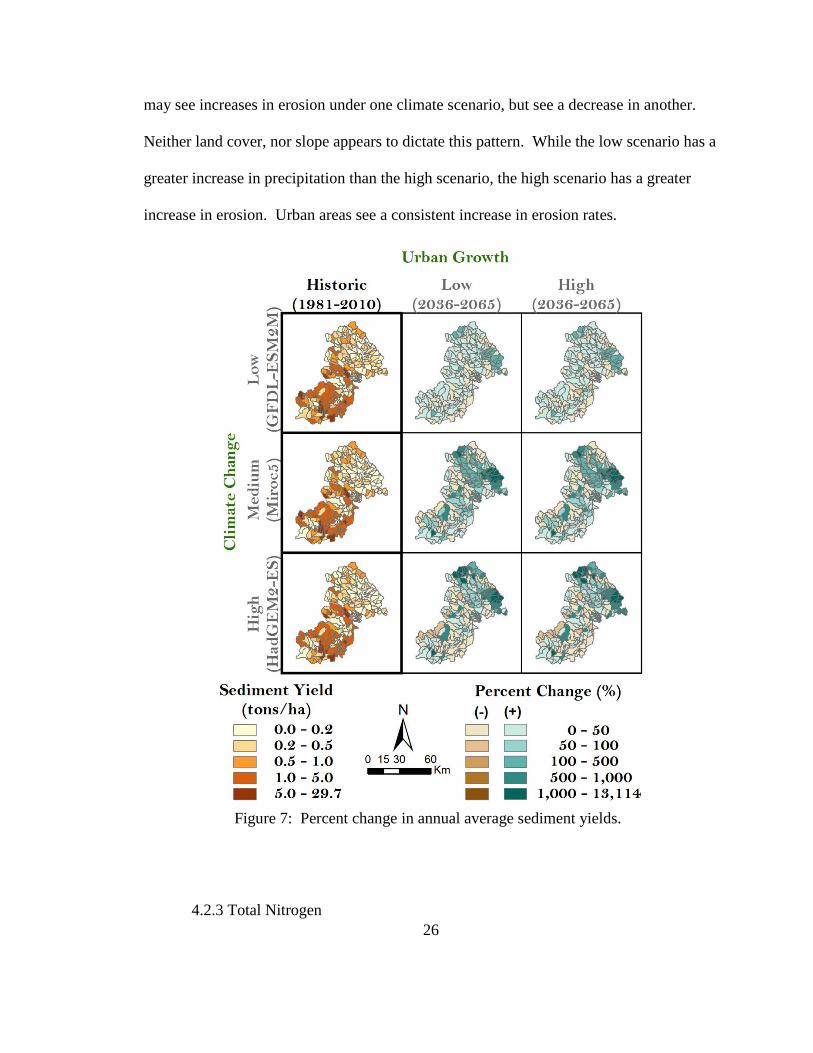
26
may see increases in erosion under one climate scenario, but see a decrease in another.
Neither land cover, nor slope appears to dictate this pattern. While the low scenario has a
greater increase in precipitation than the high scenario, the high scenario has a greater
increase in erosion. Urban areas see a consistent increase in erosion rates.
Figure 7: Percent change in annual average sediment yields.
4.2.3 Total Nitrogen

27
Total nitrogen travels to the stream through lateral flow, overland flow, and
transport with sediment. TN increases annually and during the winter for all climate
scenarios reflecting increased transport from higher flows (Table 7). The only decreases
are seen under the medium and high climate scenarios where there are decreases in
precipitation. Yamhill sees either smaller increases, or larger decreases under the high
urbanization scenarios due to conversion of high nutrient yielding lands to lower yielding
urban lands. Tualatin sees this same pattern for the medium climate scenario, but more
mixed results for the low and high scenarios.
Table 7: Percent change in annual and
seasonal TN loadings.
Tualatin Yamhill
Climate Land Use
Low High Low High
Annual
Low 13.9 13.93 4.6 4.07
Medium 48.7 48.27 21.67 21.01
High 28.15 28.26 2.78 2.20
Winter
Low 17.75 17.75 6.25 5.52
Medium 59.38 59.07 20.49 19.62
High 56.83 57.14 12.65 11.78
Summer
Low 78.6 78.61 64.6 63.88
Medium 0.002 -1.58 -31.97 -32
High -64.04 -64.24 -70.55 -70.83
Spatial patterns of TN yield show the importance of slope (Figure 8). Range
lands and lands under hay production with higher slopes produce the highest yields.
Cultivated agricultural lands lie on more gently sloping valley lands and do not

28
demonstrate as heavy an impact in the model. Urbanizing sub-basins show large
increases in nutrients. Areas which have historically low nutrient yields also see greater
proportionate increases in yields. These patterns closely follow those of sediment.
Figure 8: Percent change in annual average TN yield.
4.2.4 Total Phosphorus

29
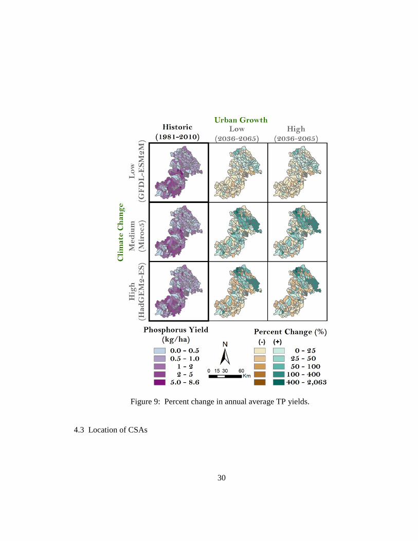
Total phosphorus travels to the stream attached to sediment, in solution with
overland flow, in mineral form, and with groundwater. The Tualatin sees annual
increases in TP throughout all climate scenarios, while Yamhill sees an increase only in
the medium scenario (Table 8). In Yamhill, the high urban growth scenarios show
slightly larger decreases in annual and winter TP loads than the low urban growth
scenario. In the summer Yamhill has slightly larger increases or slightly smaller
decreases in the high urban growth scenario. The largest increases in TP occur during the
summer in the low climate scenario due to a 30% increase in precipitation.
Spatial patterns of TP follow those of sediment. There are large increases in the
Portland metro area as well as in the higher elevations of the coast range in the Tualatin
(Figure 9) as a result of high sloping urban lands and areas harvested for timber.
Table 8: Percent change in annual and seasonal TP
loadings.
Tualatin
Yamhill
Climate Land Use
Low High Low High
Annual
Low 4.7 4.67 -15.7 -15.83
Medium 68.8 73.94 1.55 1.47
High 58.75 64.93 -17.85 -17.89
Winter
Low 1.12 1.12 -18.32 -18.51
Medium 57.11 60.9 -11.51 -11.66
High 78.77 85.13 -17.82 -17.87
Summer
Low 359 359 596.21 598.38
Medium -57.24 -52.4 -76.97 -76.08
High -77.69 -75.74 -70.8 -70.37
30
Figure 9: Percent change in annual average TP yields.
4.3 Location of CSAs

31
The top 1% of sub-basins have an average index of 19.4. The bottom 1% have an
average index of 0.05. Out of the sub-basins in the study site, the top 12% are in the
Yamhill basin, signifying the proportionately high sediment exports predicted by the
model. The top 5% index values for each basin can be visualized in Figure 9. Many
CSA’s remain the same while some hotspots shift according to the spatial patterns
created by climate change and urbanization discussed previously. The high climate
scenario sees 6 CSAs shift. The medium scenario sees 5 shift, and the low scenario sees
only 3 CSAs shift.
At the HRU level, relationships between land cover and topography can be seen
more directly than at the sub-basin scale due to averaging. Hotspots at the HRU scale
consist of high sloping hay and range land. The average basin-wide slope in Tualatin is
14.7%, while the area weighted average slope for HRU CSAs is 30.5%. In Yamhill, the
basin-wide slope is 17.3%, while the average slope for HRU CSAs is 23.7%. The
dominant land use in HRU CSAs for Tualatin is rangeland (88%) and hay (12%). The
dominant land use in HRU CSAs for Yamhill is Hay (54%) and rangeland (46%).

32
Figure 10: Shifts in hotspots due to climate change and urbanization.
4.4 Management
Application of vegetative filter strips has an average rate of reduction of 61.4%
for erosion, 49.2% for TN, and 62.9% for TP. The low flow year had a larger reduction
in sediment and nutrients (S: 65.7, TN: 51.2, TP: 65.5%) than the high flow year (S:
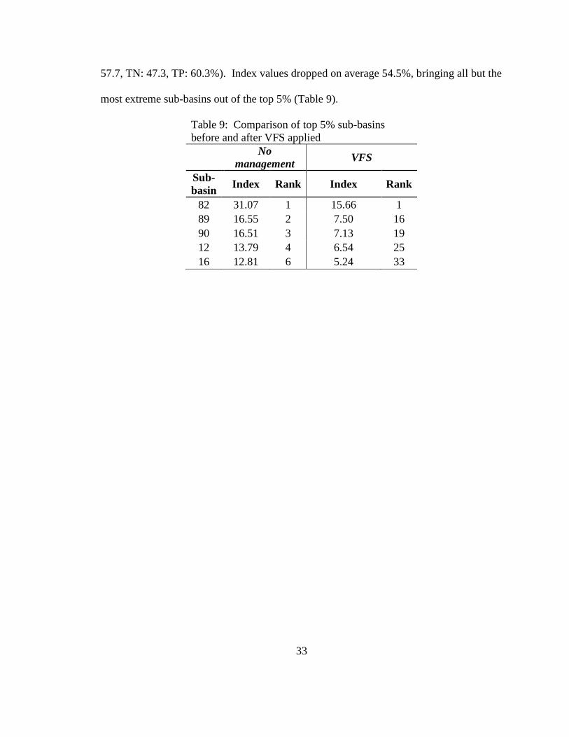
33
57.7, TN: 47.3, TP: 60.3%). Index values dropped on average 54.5%, bringing all but the
most extreme sub-basins out of the top 5% (Table 9).
Table 9: Comparison of top 5% sub-basins
before and after VFS applied
No
management VFS
Sub-
basin Index Rank Index Rank
82 31.07 1 15.66 1
89 16.55 2 7.50 16
90 16.51 3 7.13 19
12 13.79 4 6.54 25
16 12.81 6 5.24 33

34
5. Discussion
5.1 Model Calibration
Results of model calibrations were mixed (Table 4). Flow simulations track well
with observed data in both basins, and the spatial patterns of water yield make sense
given the known orographic effects of the coast range (Figure 10).
Sediment calibration in the Yamhill was acceptable. Model assessment at other
parts of the Yamhill was not possible due to lack of data, but the homogenous land cover
characteristics throughout the basin may make it safe to assume the model performs well
throughout. Sediment calibrations in the Tualatin were acceptable at the Dilley and West
Linn gage. However, the Fanno gage needs improvement. The poor performance is
likely due to SWAT’s inability to effectively capture physical processes unique to urban
areas. SWAT assumes urban areas consist of impervious surfaces and Bermuda grass.
This assumption is likely too simplistic. For example, we’d expect SWAT to under
predict sediment loads in urban areas which have yards with more exposed soils. This
may be one explanation for the negative bias in sediment results. However, this alone
cannot account for SWAT’s deficiencies in Fanno Creek since the NSE and RSR are also
poor, meaning the model is not simply under predicting, but differs erratically from the
observed data. One possible explanation is that SWAT cannot capture in-stream
processes unique to small urban watersheds. Urban streams are known to function
differently than undisturbed streams. In particular, a larger percentage of sediment

35
originates from channel erosion rather than hill slope processes (Paul and Meyer 2001).
This channel erosion can happen in response to storm events, or as a result of
construction near the stream. These types of discontinuous processes would cause
sediment loads to vary sporadically over both short and long time periods, and may
explain SWAT’s poor performance. Spatial patterns of sediment yield are sensible, but
due to the poor calibration results for Fanno Creek, the results in this part of the basin
have less certainty. As a result, our confidence in the precise changes that may take place
is smaller in Fanno Creek than in other portions of the basin.
Nutrient calibrations are acceptable for the Dilley and Yamhill DEQ calibration
points, but were unsatisfactory for the West Linn and Fanno gages. This makes sense
since there are two waste water treatment plants above the West Linn gage which release
water with varying concentrations of nutrients throughout the year. While flow from
these plants were included in the model, estimates of nutrient concentrations were
difficult to derive. As a result these sources of nutrients were excluded from the model.
This would explain the under prediction of both TN and TP at the West Linn gage. As
for Fanno Creek, since nutrients tend to travel with sediment, the poor sediment results
may also explain the poor nutrient results. Spatial patterns of nutrient yield appear
sensible in the Tualatin where yields roughly track sediment yields.
5.2 Spatial Patterns of Flow, Sediment, and Nutrients

36
The spatial patterns of SWAT output can be seen in Figure 10. These patterns
constitute a mix of natural processes, model structure, and underlying model
assumptions. Orographic effects from the Coast Range create a clear east-west gradient
in water yield with higher yields in the higher elevations to the west, and lower yields in
the valleys of the two basins. Summer water yield is larger in urban areas (Figure 6) than
the rest of the basin. One would expect baseflow in the higher elevations to sustain water
yield throughout the basin at higher levels than the urban areas. A more complete
analysis of sub-surface flows in the model could explain why this pattern is taking place.
One explanation is that baseflows during the summer are not enough to overtake the
immediate runoff that will take place in urban areas.
Figure 11: Spatial patterns of predicted flow, sediment, total
nitrogen, and total phosphorus.

37
There are intra- and inter-basin spatial patterns for sediment. Predicted terrestrial
yields in the Tualatin are uniformly smaller than those in the Yamhill. This disparity is
likely due to in-stream processes in the model not being properly calibrated. This type of
calibration could be done in the future using a submerged jet to characterize the erosion
taking place when stress is applied to the channel surface (Hanson 1990, Allen et al
1999). This is resource intensive, and results are likely to vary throughout the stream
network based on particle size distribution (Kaufmann et al 2008). It should be noted that
SWAT’s default sediment routing algorithm, the simplified Bangold equation assumes all
sediment is of silt size, and it does not partition erosion between the stream bank and
stream bed. More advanced routines are available that does take into account particle
size. However, it is still incumbent on the user to define the median particle diameter.
At the time of this writing, no field studies could be found detailing sediment
yields off the landscape. A study using the EPIC model in the Tualatin exists (Moberg
1995), but no empirical data were used. Moberg (1995) recommends further field scale
data collection, but no study has yet been completed. As a result of default in-stream
sediment processes, higher in-stream sediment yields are apportioned directly to
terrestrial erosion in this study.
Intra-basin variation is due to the combination of landscape factors such as land
uses and slopes. In the Tualatin, modeling results indicate that the majority of erosion is
due to clear-cuts located on high slopes throughout the Coast Range. Since cultivated
agricultural lands are found more frequently on low to medium slopes in the Tualatin,

38
there is less opportunity for severe erosion to take place. In the Yamhill, the most severe
erosion comes from lands classified as hay which reside on steeper slopes. In both basins
forested areas contribute least to erosion due to the soil’s thick layers of humus and
protection from rain splash erosion.
Much of the nutrient loads into streams travel either bound to colloids or in
solution with overland flow, so sub-basins with higher sediment yields also see higher
nitrogen and phosphorus yields. This explains the similar inter-basin patterns for TN and
TP. While studies have shown a relatively higher phosphorous concentration in the
Tualatin River due to naturally occurring concentrations of phosphorus in the Hillsboro
Formation (Wilson et al 1999), the similar progeny of soils extant in both basins suggest
this pattern is present in Yamhill as well (email correspondence with Scott Burns). Thus,
the inter-basin differences in phosphorus are mainly due to its relationship with sediment.
5.3 Future Changes and Adaptive Management
While there are decreases in sediment and nutrients basin-wide under some
scenarios, urban areas consistently show increases. This finding is consistent with many
previous studies (Tong and Chen 2002, Franczyk and Chang 2009, Tu 2009, Praskievicz
and Chang 2011), and emphasizes the need for adaptive policies addressing these
pollution sources.
The wide range of responses to climate scenarios points to the uncertainty
inherent in climate models, and the corresponding hydrological response to these

39
changes. Non-linear effects such as summertime increases in flow despite summertime
reductions in precipitation in the medium scenario highlight some unexpected changes
that may take place. This wide variation stresses the need for managers to develop
adaptive plans which incorporate these uncertainties while scientists work to develop
climate models with less uncertainty.
This study demonstrates the ability of SWAT to locate CSAs, and visualize how
they may change in the future. Due to this model’s limitation in how it represents land
cover, and a lack of research validating CSAs identified by SWAT (Niraula et al. 2013),
more research is needed before these CSAs can be used to guide regulatory activities.
The application of VFS clearly demonstrates the advantage of best management
practices, whether the issue being addressed is urban growth, or agricultural runoff. This
research suggests that VFS could be used as a method of promoting sustainable land
management practices.
40
6. Conclusions
Changes in precipitation levels and urban growth are two main drivers that
threaten watershed health in the future. This study focusses on assessing hydrologic and
water quality changes to precipitation and urban growth, and investigates how the
application of vegetative filter strips might ameliorate these effects.
Flows typically follow precipitation trends, but some non-linear effects result
from seasonal soil water storage permitting summer flows to increase despite reductions
in summer rains. Urban areas show larger increases in flows due to high percentages of
impervious surfaces. Winter flow changes are similar to annual changes.
As flow increases, sediment yields increase basin-wide in most scenarios. Urban
areas display particular sensitivity to increases in sediment yields, possibly due to their
historically small yields relative to other land uses. TN yields increase basin-wide in
most scenarios. High sloping regions with hay and rangelands have the highest TN
yields. Urban areas show the greatest sensitivity to future climate and land use change.
TP yields increase in exactly half of the scenarios, however the percent increases in these
scenarios is greater than the decreases. Spatial patterns follow those of sediment. The
greatest increases can be seen in urban lands. These findings suggest that urban areas can
be targeted for reducing high flows and additional nutrient and sediment loads.
CSAs are located in areas of high slopes and hay or range lands. CSAs shift
under urban growth and climate change suggesting that managers could use models to
identify areas deserving extra regulatory attention; however validation through field
41
studies is required before model output can be trusted. Changes in CSAs appear to be
related more to climate change than urban growth in this study. Implementation of VFS
reduced sediment and nutrient loads to the stream suggesting this should be promoted as
a best management practice for land owners.
The results of this study suggest that SWAT is a useful tool for identifying target
areas for reducing nutrient and sediment loads and evaluating the effects of alternative
land management on nutrient and sediment loads under the pressure of climate change
and urban growth. Future studies should focus on validating CSAs identified by SWAT
and characterizing downstream effects resulting from best management practices.
42
7. References Cited
Abatzoglou, J.T. 2013. Development of gridded surface meteorological data for
ecological applications and modeling. International Journal of Climatology 33:121-131.
Abatzoglou, J.T., and Brown, T.J. 2012. A comparison of statistical downscaling
methods suited for wildfire applications. International Journal of Climatology 32: 772-
780.
Abu-Zreig, M., Rudra, R.P., Whiteley, H.R., Lalonde, M.N., and Kaushik, N.K. 2003.
Phosphorus removal in vegetated filter strips. Journal of Environmental Quality 32:613-
619.
Abu-Zreig, M., Rudra, R.P., Lalonde, M.N., Whiteley, H.R., and Kaushik, N.K. 2004.
Experimental investigation of runoff reduction and sediment removal by vegetated filter
strips. Hydrological Processes 18:2029-2037.
Allen, P.M, Arnold, J., Jakubowski, E. 1999. Prediction of stream channel erosion
potential. Environmental and Engineering Geoscience 5:339-351.

43
Arnold, J.G., Srinivasan, R., Muttiah, R.S., and Williams, J.R. 1998. Large area
hydrologic modeling and assessment part I: Model Development. Journal of the
American Water Resources Association 34(1):73-89.
Arnold, J.G., Moriasi, D.N., Gassman, P.W., Abbaspour, K.C., White, M.J., Srinivasan,
R., Santhi, C., Harmel, R.D., van Griensven, A., Van Liew, M.W., Kannan, N., and Jha,
M.K. 2012. SWAT: Model use, calibration, and validation. Transactions of the ASABE
55(4):1491-1508.
Atasoy, M., Palmquist, R.B., Phaneuf, D.J. 2006. Estimating the effects of urban
residential development on water quality using microdata. Journal of Environmental
Management 79:399-408.
Boeder, M., H. Chang. 2008. Multi-scale analysis of oxygen demand trend in an
urbanizing Oregon watershed. Journal of Environmental Management 400(1-3): 567-
581.
Brown, L.C. and Barnwell Jr., T.O. 1987. The enhanced water quality models QUAL2E
and QUAL3E-UNCAS documentation and user manual. EPA document EPA/600/3-
87/007. USEPA, Athens, GA.

44
Chang, H., Evans, B.M., and Easterling, D.R. 2001. The effects of climate change on
stream flow and nutrient loading. Journal of the American Water Resources Association
37(4):973-985.
Chang, H. 2004. Water quality impacts of climate and land use changes in southeastern
Pennsylvania. The Professional Geographer 56(2):240-257.
Chang, H., and Jung, I-W. 2010. Spatial and temporal changes in runoff caused by
climate change in a complex large river basin in Oregon. Journal of Hydrology 388(3-
4):186-207.
City of McMinville [Data]. (2011). http://www.ci.mcminnville.or.us/
CWS (Clean Water Services) [Data]. 2011. 16060 SW 85th Ave, Tigard, OR 97224.
Choi, W. 2008. Catchment-scale hydrological response to climate-land-use combined
scenarios: A case study for the Kishwaukee River Basins, Illinois. Physical Geography
29(1):79-99.
Ferrari, R.L. 2001. Henry Hagg Lake 2001 Survey. Sedimentation and River Hydraulics
Group. Denver, Co.

45
Franczyk, J., and Chang, H. 2009. The effect of climate change and urbanization on the
runoff of the Rock Creek basin in the Portland metropolitan area, Oregon, USA.
Hydrological Processes 23:805-815.
Hanson, G.J. 1990. Surface erodibility of earthen channels at high stresses. Part II-
Developing an in situ testing device. Transactions of ASAE 33:132-137.
Hoyer M. 2013. Scenario Development and Analysis of Freshwater Ecosystem Services
under Land Cover and Climate Change in the Tualatin and Yamhill River Basins, Oregon.
Master’s thesis. Portland State University.
Hoyer M, Chang H. 2014. Development of future land cover change scenarios in the
metropolitan fringe, Oregon, U.S.A. with a participatory element (in review).
Kaufmann, P.R., Faustini, J.M., Larsen, D.P., Shirazi, M.A. 2008. A roughness-corrected
index of relative bed stability for regional stream surveys. Geomorphology 99:150-170.
MACA (Multivariate Adaptive Constructed Analogs) Statistical Downscaling Method
[Data]. 2013. Data Retrieved from: http://nimbus.cos.uidaho.edu/MACA/
Meyer, J.L., Paul, M.J., and Taulbee, W.K. 2005. Stream ecosystem function in
urbanizing landscapes. Journal of the North American Benthological Society 24(3):602-
612.

46
Moberg, D. 1995. Tualatin basin farm effects on runoff quality. Part III: EPIC Model
Predictions. USDA – Natural Resources Conservation Service.
Moriasi, DN, Arnold, J.G., Van Liew, M.W., Bingner, R.L., Harmel, R.D., Veith, T.L.
2007. Model evaluation guidelines for systematic quantification of accuracy in watershed
simulations. Transactions of the ASABE 50(3):885-900.
Munoz-Carpena R., Parsons, J.E. 1999. Modeling hydrology and sediment transport in
vegetative filter strips. Journal of Hydrology 214:111-129.
Neitsch, S.L., J.G. Arnold, J.R. Kiniry, J.R. Williams. 2011. Soil and Water Assessment
Tool Theoretical Documentation Version 2009. Texas Water Resources Institute
Technical Report No. 406.
NHD (National Hydrography Dataset) Plus (Version 1) [Data]. 2010. Retrieved from
http://www.horizon-systems.com/nhdplus/
Niraula R., Kalin, L., Srivastava, P., Anderson, C.J. 2013. Identifying critical source
areas of nonpoint source pollution with SWAT and GWLF. Ecological Modelling
268:123-133.

47
Oregon Department of Environmental Quality (ODEQ) 2012 [Data]. Provided by
Eugene Foster from LASAR Database: deq12.deq.state.or.us/lasar2/
Oregon Department of Environmental Quality (ODEQ) 2001. Tualatin Sub-basin Total
maximum Daily Load (TMDL):
http://www.deq.state.or.us/wq/tmdls/docs/willamettebasin/tualatin/tmdlwqmp.pdf. Last
accessed 3/1/2013.
Paul, M.J., and Meyer, J.L. 2001. Streams in the urban landscape. Annual Review of
Ecology, Evolution, and Systematics 32:333-365.
Praskievicz, S., and Chang, H. 2011. Impacts of climate change and urban development
on water resources in the Tualatin River Basin, Oregon. Annals of the Association of
American Geographers 101(2):249-271.
Pratt, B., and Chang, H. 2012. Effects of land cover, topography, and built structure on
seasonal water quality at multiple scales. Journal of Hazardous Materials 209/210:48-58.
Randall, G.W., and Mulla, D.J. 2001. Nitrate nitrogen in surface waters as influenced by
climatic conditions and agricultural practices. Journal of Environmental Quality 30:337-
344.
48
Runkel, R.L., Crawford, C.G., and Cohn, T.A. 2004. Soad Estimator (LOADEST): A
FORTRAN program for estimating constituent loads in streams and rivers. In Techniques
and Methods Book 4. USGS. Reston, VA.
Soil Conservation Service. 1972. Section 4: Hydrology In National Engineering
Handbook. SCS.
STATSGO (State Soil Geographic) Database [Data]. 2010. Included in SWAT model
download: http://swat.tamu.edu/
Sullivan, A.B., and Rounds. S.A. 2005. Modeling hydrodynamics, temperature, and water
quality in Henry Hagg Lake, Oregon, 2000-03. U.S. Geological Survey Scientific
Investigations Report 2004-5261 38 p.
Tang, Z., Engel, B.A., Pijanowski, B.C., Lim, K.J. 2005. Forcasting land use change and
its environmental impact at a watershed scale. Journal of Environmental Management
76:35-45.
Tong, S.T.Y., and Chen, W. 2002. Modeling the relationship between land use and
surface water quality. Journal of Environmental Management 66:377-393.
49
Tu, J. 2009. Combined impact of climate and land use changes on streamflow and water
quality in eastern Massachusetts, USA. Journal of Hydrology 379:268-283.
USGS (US Geological Survey). US Land cover. 2011. Retrieved from The USGS Land
Cover Institute's website: http://landcover.usgs.gov/uslandcover.php.
USGS (US Geological Survey). National Water Information System (NWIS). 2012.
http://waterdata.usgs.gov/nwis/
Vorosmarty, C.J., Green, P., Salisbury, J., and Lammers, R.B. 2000. Global water
resources: Vulnerability from climate change and population growth. Science 289:284-
288.
Walch, C.J., Roy, A.H., Feminella, J.W., Cottingham, P.D., Groffman, P.M., and Morgan
II, R.P. 2005. Journal of the North American Benthological Society 24(3):706-723.
White, M.J., and Arnold, J.G. 2009. Development of a simplistic vegetative filter strip
model for sediment and nutrient retention at the field scale. Hydrological Processes
23:1602-1616.
50
Whitehead, P.G., Wilby, R.L., Battarbee, R.W., Kernan, M., and Wade, A.J. 2009. A
review of the potential impacts of climate change on surface water quality. Hydrological
Sciences Journal 54(1):101-123.
Williams, J.R. 1975. Sediment-yield prediction with universal equation using runoff
energy factor. P. 244-252. In Present and prospective technology for predicting sediment
yield and sources: Proceedings of the sediment-yield workshop, USDA Sedimentation
Lab., Oxford, MS, November 28-30, 1972. ARS-S-40.
Wilson, D.C., Burns, S.F., Jarrell, W., Lester, Alan, and Larson, E. 1999. Natural ground-
water discharge of orthophosphate in the Tualatin Basin, Northwest Oregon.
Environmental & Engineering Geoscience 5(2):189-197.

51
Appendix A: Model Configuration
The Tualatin is a complicated basin to model due to the high level of management
taking place. Because of this, a significant amount of time was spent finding and
formatting data for input into SWAT and devising ways to incorporate various features of
the basin. One example of this is the Henry Hagg Lake Reservoir. In order to configure
SWAT to include the reservoir, the automated sub-basin delineation based on the stream
network had to be manually re-configured. This change can be seen in Figure A.1. The
USGS gage along Scoggins Creek and the USGS gage along Sain Creek were used as
points to demarcate upstream sub-basins from Hagg Lake.
Figure A.1: Sub-basin delineation around Henry Hagg Lake had to be
manually adjusted for a realistic representation of the spatial extent of the
reservoir.
A second example is HRU definition. SWAT permits thresholds to be set to limit
the size and complexity of the model. HRUs are composed of slope, soil, and land cover,
and a threshold can be set for each. For example, if the land cover threshold is set to 20%
and a sub-basin contains:

52
10% Cultivated Crops,
30% Hay,
25% Urban-Low density,
15% Forest-Evergreen,
10% Urban-Industrial,
10% Urban-Medium density,
Hay, and Urban-Low density would be reapportioned so that
Hay = (30%/55%)*100 = 54.55%, and
Urban-Low density = (25%/55%)*100 = 45.45% .
SWAT documentation says “The threshold levels set for multiple HRUs is a
function of the project goal and the amount of detail desired by the modeler. For most
applications, the default settings for land use threshold (20%) and soil threshold (10%)
and slope threshold (20%) are adequate.” (Winchell et al. 2010, pg. 131-132). For this
thesis I used the default settings since future land cover scenarios had not yet been
finalized during model construction. Since urban lands comprise small portions of the
basin, these settings are problematic, as can be seen by the mostly similar outputs for
both land covers. Furthermore, where changes in land cover are significant enough to
reach the threshold, unusual changes in sub-basin level output can be seen as a result of a
new land cover’s inclusion in that sub-basin where it had been excluded previously.
While these threshold levels are useful for simplifying the model and reducing run-time,
given the scope of this research, a more moderate threshold should have been set for land

53
cover and the additional option of exempting certain land covers from this threshold
should have been applied to all urban lands.

54
Appendix B: Sensitivity Analysis, Calibration, and Validation
Sensitivity Analysis was performed for many parameters in both the Tualatin and
Yamhill basins. The SWAT-CUP software provides automated routines and graphical
output which enables detailed inspection of a parameter’s sensitivity (Abbaspour 2012).
An example of parameter sensitivity for EPCO (Plant uptake compensation factor), can
be seen in figure B.1. This parameter demonstrates slight changes to wintertime peaks,
but is otherwise insensitive. Sensitivity analysis was done for 43 parameters.
Sensitivities for select parameters can be seen in Table B.1.
Figure B.1: Sensitivity analysis of the EPCO parameter.

55
Table B.1: List of final calibrated parameters for Tualatin and Yamhill sub-basins
Description Parameter Min Max
Sensitivity
([I]ncrease,
[D]ecrease)
Flow
Baseflow alpha factor
(days)
v__ALPHA_BF.gw
* 0 1
Wet season: I
Dry season: D
Soil evaporation
compensation factor v__ESCO.bsn 0.01 1 I
Plant uptake
compensation factor v__EPCO.bsn 0 1 D
Available water capacity
of the soil layer r__SOL_AWC().sol -0.2 0.2 D
Treshold depth of water
in the shallow aquifer
required for return flow
to occur (mm)
v__GWQMN.gw 0 5000 D
Sediment
Average slope length r__SLSUBBSN.hru 10 150 I
Min value of USLE C
factor applicable to the
land cover/plant (Forest)
r__USLE_C.crop.da
t
0.00
1 0.5 I
USLE equation soil
erodibility (K) factor r__USLE_K().sol 0 0.65 I
Average Slope
Steepness r__HRU_SLP.hru 0 1 I
Nitrogen
Nitrogen percolation
coefficient v__NPERCO.bsn 0.1 1 I
Denitrification
exponential rate
coefficient
v__CDN.bsn 0.1 3 I
Denitrification threshold
water content v__SDNCO.bsn 0.1 1 D
*v: Parameter is assigned this value. r: Parameter is multiplied by 1 + this value.
LOADEST models had largely good model fit statistics. It should be noted,
however, that these estimates were done using load rather than concentration, and thus
suffer from spurious correlation since flow is used in both the independent and dependent

56
variables (Shivers and Moglen 2008). A summary of LOADEST model results can be
seen in Table B.2.
Table B.2: LOADEST sediment and nutrient results.
Parameter Calibration
Period
Grab
Samples
Estimation
Period NSE PBIAS R
2
Tualatin River at West Linn
TSS 1988 – 2010 828 1981 – 2010 0.06 11.14 0.94
TN 1974 – 2002 545 1981 – 2010 0.93 0.12 0.95
TP 1974 – 2010 972 1981 – 2010 0.65 5.63 0.92
Tualatin River at Dilley
TSS 1984 – 2011 1014 1981 – 2010 0.45 -10.24 0.89
TN 1984 – 2011 1,007 1981 – 2010 0.68 3.15 0.88
TP 1984 – 2011 1,032* 1981 – 2010 0.67 -2.80 0.84
Fanno Creek at Durham
TSS 10/1/1993 –
2012 530
10/1/1993 –
2010 -1.76 46.09† 0.93
TN 10/1/1993 –
2012 623**
10/1/1993 –
2010 0.93 2.72 0.98
TP 10/1/1993 –
2012 733
10/1/1993 –
2010 0.66 1.75 0.98
Yamhill Water Quality Station
TSS 10/1/1994 –
2012 164
10/1/1994 –
2010 0.72 3.58 0.96
TN 10/1/1994 –
2007 132
10/1/1994 –
2010 0.77 8.86 0.97
TP 10/1/1994 –
2012 164
10/1/1994 –
2010 0.85 -1.74 0.97
* 25 samples registered below
hardware detection limits
** 1 sample registered below
hardware detection limits
† LOADEST does not recommend
using models with PBIAS greater
than 25%
SWAT model fit was measured using both statistical and visual inspection.
Visual demonstration of model fit was not able to be included in the main document due

57
to space constraints, so they are provided here in Figure B.2. While model fit is generally
good, the model at times underestimates nutrient loads. Whether these disparities are due
to inaccurate LOADEST estimates, or model construction is difficult to say.

58

59
Figure B.2: Time series of calibrated and validated results for both the Tualatin and
Yamhill sub-basins.
60
Appendix C: Uncertainty
A formal uncertainty analysis was not conducted for this study, so what follows is
a brief discussion of the various sources of uncertainty. The uncertainty in watershed
modeling can be categorized into 3 types. Measurement uncertainty derives from the
uncertainty inherent in the field collected “observed” data used to calibrate a model.
Measurement uncertainty can be estimated using the detection limits of the hardware
used to make field observations. In our study the USGS and DEQ flow, sediment and
nutrient data fall under this category. The LOADEST model estimates also fall under
this category.
The second type is model uncertainty and derives from the fact that no model
incorporates all physical processes, nor are all physical processes known to us. An
example of this kind of uncertainty is the “second storm” effect, where sediment and
nutrients are flushed through the system by a rain storm, so that concentrations in a
follow up storm are over-estimated.
The third type is parameter uncertainty and derives from the spatial and temporal
variation in parameters used to calibrate the model. Many parameters are difficult to
measure empirically, and so the inverse modeling technique is used to estimate the value
of these parameters (Abbaspour et al. 1999). However, the non-uniqueness, or
equifinality problem, where different combinations of parameters can result in the same
model output prevent a clear method for acquiring the true parameter values (Abbaspour
2012). Parameter uncertainty can be estimated by measuring the model response to
various parameter inputs. This analysis is computationally intensive and requires over

61
500 model runs. It also requires the modeler to select realistic parameter ranges, a figure
which may change depending on the experience level of the modeler, and the modeler’s
familiarity with the study site.

62
Appendix D: Historic and Future Climate
Historic summaries of climate in the two basins based off of data provided by
Abatzoglou (2013) had to be removed from the main document but can be seen in Figure
D.1. Spatial distribution of the gridded future climate scenarios for annual and seasonal
scales can be seen in Figure D.2.
Figure D1: Hydroclimate in the (a) Tualatin and (b) Yamhill sub-basins, 1995-2010
Water year

63
Figure D.2: Spatial distribution of annual and seasonal changes to precipitation in each
of the three climate scenarios.
References Cited
Abatzoglou, J.T. 2013. Development of gridded surface meteorological data for
ecological applications and modeling. International Journal of Climatology 33:121-131.
64
Abbaspour, K.C., Sonnleitner, M.A., Schulin, R. 1999. Uncertainty in estimation of soil
hydraulic parameters by inverse modeling: Example lysimeter experiments. Soil Science
Society of America Journal 63:501–509.
Abbaspour, K.C. 2012. SWAT-CUP 2012: SWAT Calibration and uncertainty programs
– A user manual. EAWAG.
Shivers, D.E., and Moglen, G.E. 2008. Spurious correlation in the USEPA rating curve
method for estimating pollutant loads. Journal of Environmental Engineering 134:610-
618.
Winchell, M., Srinivasan, R., Di Luzio, M., Arnold, J. 2010. ArcSWAT Interface for
SWAT 2009 User’s Guide. Blackland Research Center. Temple, Texas.
Recommended


![Student’s t Sensitivities: GreeksfortheGossetFormulaearXiv:1003.1344v2 [q-fin.PR] 16 Jul 2010 Student’st-DistributionBasedOption Sensitivities: GreeksfortheGossetFormulae Daniel](https://img.pdfslide.us/doc/110x75/5fa1f5e65b7bfb78540e321a/studentas-t-sensitivities-greeksforthegossetformulae-arxiv10031344v2-q-finpr.jpg)