arX
iv:h
ep-t
h/02
1202
1v3
12
Jan
2004
HUTP-02/A062hep-th/0212021
Large Volume Perspective on Branes at Singularities
Martijn Wijnholt
Jefferson Laboratory of Physics, Harvard University
Cambridge, MA 02138, USA
Abstract
In this paper we consider a somewhat unconventional approach for deriving worldvolume
theories for D3 branes probing Calabi-Yau singularities. The strategy consists of extrapo-
lating the calculation of F-terms to the large volume limit. This method circumvents the
inherent limitations of more traditional approaches used for orbifold and toric singularities.
We illustrate its usefulness by deriving quiver theories for D3 branes probing singularities
where a Del Pezzo surface containing four, five or six exceptional curves collapses to zero
size. In the latter two cases the superpotential depends explicitly on complex structure
parameters. These are examples of probe theories for singularities which can currently not
be computed by other means.
December 2002

Contents
1. Overview . . . . . . . . . . . . . . . . . . . . . . . . . . . . . . . . . . . 1
2. Large volume perspective . . . . . . . . . . . . . . . . . . . . . . . . . . . . 3
2.1. Relation to exceptional collections . . . . . . . . . . . . . . . . . . . . . . 3
2.2. Spectrum and quiver diagram . . . . . . . . . . . . . . . . . . . . . . . . 4
2.3. Superpotential . . . . . . . . . . . . . . . . . . . . . . . . . . . . . . . 7
2.4. Mutations and Seiberg duality . . . . . . . . . . . . . . . . . . . . . . . . 9
3. Superpotentials for toric and non-toric Calabi-Yau singularities . . . . . . . . . . . 12
3.1. Del Pezzo 3 . . . . . . . . . . . . . . . . . . . . . . . . . . . . . . . . 14
3.2. Del Pezzo 4 . . . . . . . . . . . . . . . . . . . . . . . . . . . . . . . . 17
3.3. Del Pezzo 5 . . . . . . . . . . . . . . . . . . . . . . . . . . . . . . . . 22
3.4. Del Pezzo 6 . . . . . . . . . . . . . . . . . . . . . . . . . . . . . . . . 26
3.5. Simple quiver diagrams for the remaining Del Pezzo’s . . . . . . . . . . . . . . 29
3.6. Preliminary remarks on the conifold . . . . . . . . . . . . . . . . . . . . . 32
3.7. Zk orbifolds . . . . . . . . . . . . . . . . . . . . . . . . . . . . . . . . 32
1. Overview
The description of certain extended objects in string theory as Dirichlet branes [1] has
given us a new window into the physics of highly curved geometries. The worldvolume
theory of a D-brane probing an orbifold singularity at low energies is described by a gauge
theory of quiver type [2]. The correspondence goes both ways; on the one hand, we can
access distance scales that are shorter than the scales we can probe with closed strings.
On the other hand, one may view this as a way of engineering interesting gauge theories
in string theory, and then using string dualities we can sometimes learn new things about
gauge theories. Let us focus on D3 branes probing Calabi-Yau three-fold singularities,
which give rise to N = 1 gauge theories in 3+1 dimensions.
Orbifolds of flat space constitute an interesting and computationally convenient set of
singular space-times, and have given us a nice picture of the probe brane splitting up into
fractional branes near the singularity1. But they are certainly not the most general type
of singularity and do not lead to the most general allowed gauge theory. Another class is
that of toric singularities, which contains the class of abelian orbifold singularities. These
backgrounds are described by toric geometry (or linear sigma models). Adding some probe
1 These are the analogues of wrapped branes when we resolve the singularity and go to large
volume.
1
branes filling the remaining transverse dimensions leads to SUSY quiver theories where the
ranks of the gauge groups are all equal and the superpotential can be written in such a
way that no matter field appears more than twice. The prime example of this type of
singularity is the conifold.
The way one usually analyses toric singularities is by embedding them in an orbifold
singularity, which we know how to deal with [3]. Then one may partially resolve the
singularity in a toric way to get the desired space. In the gauge theory this corresponds
to giving large VEVs to certain fields and integrating out the very massive modes. At
sufficiently low energies the gauge theory only describes the local neighbourhood of the
toric singularity.
This however does not yet exhaust the class of allowed Calabi-Yau singularities or
N = 1 gauge theories. We refer to the remaining cases as non-toric singularities.
In this article we would like to attack these cases by using an approach different from
the ones we have mentioned above. The strategy consists of extrapolating to large volume
where the correct description of the fractional branes is in terms of certain collections
of sheaves2, called exceptional collections. The matter content and superpotential can
be completely determined by geometric calculations involving these collections, and the
results are not affected by the extrapolation. In principle this yields a general approach to
all Calabi-Yau singularities, both toric and non-toric.
In the next section we will review many of the ingredients of this approach3. In the
following section we will apply the techniques to compute the quiver theories for branes
probing certain Calabi-Yau geometries where a four-cycle collapses to zero size. If the
singularity can be resolved by a single blow-up, such a four-cycle is either a P1 fibration
over a Riemann surface or a Del Pezzo surface. We will treat some toric and non-toric Del
Pezzo cases in detail, computing their moduli spaces and showing how they are related to
known quiver theories through the Higgs mechanism. The non-toric cases considered here
are new and there is no other method we know of for calculating them. The case of Del
Pezzo 6 in particular can be viewed as a four parameter non-toric family of deformations
of the familiar C3/Z3 × Z3 orbifold singularity.
In order to do the computations we introduce the notion of a ‘three-block’ quiver
diagram in section three. Quiver diagrams of this type have some important simplifying
2 For our purposes these will mostly be ordinary vector bundles, even line bundles.3 Some references: [4,5,6,7,8,9]
2
features. Most importantly for our purposes is that they they lead to superpotentials with
only cubic terms for all the Del Pezzo cases. Other quiver theories may then be deduced
through Seiberg duality.
2. Large volume perspective
2.1. Relation to exceptional collections
We will start with a non-compact Calabi-Yau threefold which has a 4-cycle or 2-cycle
shrinking to zero size at a singularity. Then we may put a set of D3 branes at the singularity
and try to understand the low energy worldvolume theory on the D3 branes, which turns
out to be an N = 1 quiver gauge theory. The analysis may be done using exceptional
collections living on the shrinking cycle.
We recall first the definition of an exceptional collection. An exceptional sheaf is
a sheaf E such that dim Hom(E,E) = 1 and Extk(E,E) is zero whenever k > 0.
An exceptional collection is an ordered collection Ei of exceptional sheaves such that
Extk(Ei, Ej) = 0 for any k whenever i > j. We will usually assume an exceptional collec-
tion to be complete in the sense that the Chern characters of the sheaves in the collection
generate all the cohomologies of the shrinking cycle 4.
A sheaf living on a cycle inside the Calabi-Yau gives rise to a sheaf on the Calabi-Yau
by “push-forward.” Heuristically this just means that we take the sheaf on the cycle and
extend it by zero to get a sheaf denoted by i∗E on the CY. An exceptional collection lifts
to a set of sheaves with “spherical” cohomology on the Calabi-Yau: because of the formula
Extk(i∗Ei, i∗Ej) ∼∑
l+m=k
Extl(Ei, Ej ⊗ ΛmN) (2.1)
where N is the normal bundle to the cycle we conclude that the cohomologies of an
exceptional sheaf are given by dim Extk(i∗E, i∗E) = 1, 0, 0, 1 for k = 0, 1, 2, 3. The
reason for the terminology is that under mirror symmetry such sheaves get mapped to
Lagrangian 3-spheres. The ordering of the sheaves is related to the ordering with respect
to the imaginary coordinate on the W -plane.
4 A more precise definition would probably be that the collection generates the bounded
derived category of coherent sheaves.
3
MKahler
:
VolumeLarge
fig. 1: Extrapolation to large volume in order to perform calculations.
The significance of exceptional collections is that the sheaves in the collection have
the right properties to be the large volume descriptions of the fractional branes at the
singularity. Since we are in type IIB string theory, D-branes filling the 3+1 flat directions
must wrap even dimensional cycles in the CY, and therefore strings ending on such branes
satisfy boundary conditions that allow for a B-type topological twist. Correlation functions
in the twisted theory are independent of the choice of Kahler structure on the Calabi-Yau,
and correspond to superpotential terms in the untwisted theory. The upshot is that Kahler
parameters only manifest themselves in the D-terms of the gauge theory. So as long as we
are asking questions only about the F-terms (superpotential terms), we can do a Kahler
deformation to give the vanishing cycle a finite volume. At large volume we can describe
D-branes as sheaves and the computations can be done using exceptional collections. It
is important to remember that the gauge theory we will be discussing doesn’t actually
live at large volume, but using the justification above we will interpret the results of the
geometric computations as protected quantities in a gauge theory which is a valid low
energy description of the D3 branes at small volume.
2.2. Spectrum and quiver diagram
In order to describe the gauge theory on the D3 branes we need to construct the D3
brane out of the fractional branes and find the lightest modes. A D3 brane filling the 3+1
flat directions is determined by specifying a point p on the Calabi-Yau, so we will use a
skyscraper sheaf Op to represent it. The RR charges of a brane are combined in the Chern
4
character of a sheaf, so if Ei is an exceptional collection and ni the multiplicities of the
fractional branes then we have the condition:
∑
i
ni ch(i∗Ei) = ch(Op). (2.2)
Notice that some of the ni are necessarily negative, because we have to cancel all the
charges associated with wrappings of 2- and 4-cycles. So it may appear that we have both
“branes” and “anti-branes” present and therefore break supersymmetry, however this is
just an artefact of the large volume description. As we vary the Kahler moduli to make
the Calabi-Yau singular the central charges5 of the fractional branes all line up and thus
they all break the same half of the supersymmetry at the point of interest6.
Now the lightest modes for strings with both endpoints on the same fractional brane
fit in an N = 1 vector multiplet. Since the fractional brane is rigid (Ext1(E,E) = 0 from
the sheaf point of view) we do not get any adjoint chiral multiplets describing deformations
from these strings. If the fractional brane has multiplicity |ni| then the vector multiplet
will transform in the adjoint of U(|ni|).
We can also have strings with endpoints on different fractional branes Ei and Ej. The
lightest modes of these strings are N = 1 chiral fields transforming in the bifundamental
of the gauge groups associated with the two fractional branes. To count their number
we can do a computation in the B-model which we can perform at large volume. If the
branes fill the whole Calabi-Yau then the ground states of these strings can be seen to
arise from the cohomology of the Dolbeault operator coupled to the gauge fields of the
two fractional branes, Q = ∂z + A(j)z − A
(i)Tz , acting on the space of anti-holomorphic
forms Ω(0,·)(E∗i ⊗ Ej). If the branes are wrapped on lower dimensional cycles then we
can dimensionally reduce by changing the gauge fields with indices that do not lie along
the worldvolume of the branes into normal bundle valued scalars. Schematically then
the number of chiral fields is in one to one correspondence with the generators of the
sheaf cohomology groups H(0,m)(E∗i ⊗ Ej ⊗ ΛnN) where N is the normal bundle of the
shrinking cycle that both branes are wrapped on, or more generally the global Ext groups
Extk(i∗Ei, i∗Ej) [10]. However we are double counting because given a generator we can
get another one by applying Serre duality on the three-fold. As we discuss momentarily the
5 The central charge is associated with a particle, not with a space-filling brane, but the two
systems are closely related as far as SUSY properties is concerned so we will borrow the language.6 A nice picture of this for the case of C3/Z3 can be found in [9].
5
corresponding physical mode would have opposite charges and opposite chirality, so this
should be part of the vertex operator for the corresponding anti-particle. Then we should
have only one chiral field for each pair of generators that are related by Serre duality.
Finally the degree of the Ext group indicates ghost number k of the topological vertex
operator. In the physical theory this gets related to the chirality of the multiplet through
the GSO projection. If the degree is even we get say a left handed fermion so we should
assign fundamental charges for the jth gauge group and anti-fundamental charges of the
ith gauge group to the chiral field. Then if k is odd we get a right handed fermion and we
should assign the opposite charges to the chiral field. The chirality flips if we turn a brane
the string ends on into an anti-brane (or more precisely if we invert its central charge)
because this shifts k by an odd integer.
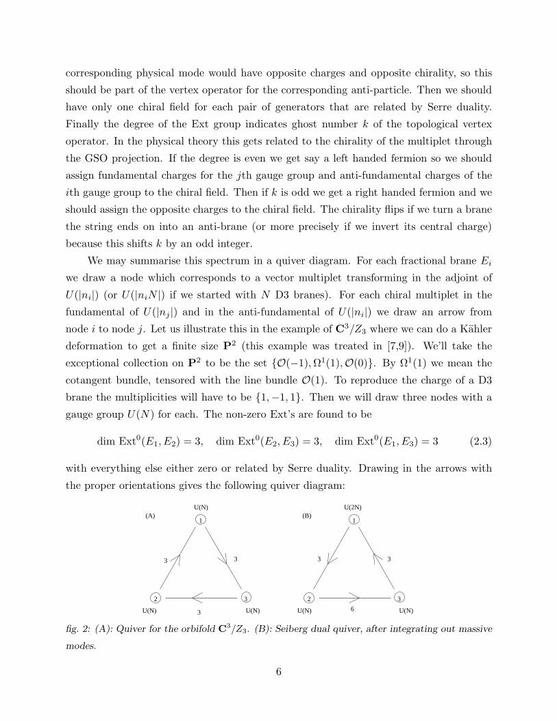
We may summarise this spectrum in a quiver diagram. For each fractional brane Ei
we draw a node which corresponds to a vector multiplet transforming in the adjoint of
U(|ni|) (or U(|niN |) if we started with N D3 branes). For each chiral multiplet in the
fundamental of U(|nj|) and in the anti-fundamental of U(|ni|) we draw an arrow from
node i to node j. Let us illustrate this in the example of C3/Z3 where we can do a Kahler
deformation to get a finite size P2 (this example was treated in [7,9]). We’ll take the
exceptional collection on P2 to be the set O(−1),Ω1(1),O(0). By Ω1(1) we mean the
cotangent bundle, tensored with the line bundle O(1). To reproduce the charge of a D3
brane the multiplicities will have to be 1,−1, 1. Then we will draw three nodes with a
gauge group U(N) for each. The non-zero Ext’s are found to be
dim Ext0(E1, E2) = 3, dim Ext0(E2, E3) = 3, dim Ext0(E1, E3) = 3 (2.3)
with everything else either zero or related by Serre duality. Drawing in the arrows with
the proper orientations gives the following quiver diagram:
1
2 3
(A) (B)
6
33
1
2 3
3 3
3 U(N) U(N)
U(N)
U(N)
U(2N)
U(N)
fig. 2: (A): Quiver for the orbifold C3/Z3. (B): Seiberg dual quiver, after integrating out massive
modes.
6
If one is only interested in the net number of arrows between two nodes, it is sufficient
to find the relative Euler character of the two corresponding sheaves
χ(i∗E, i∗F ) =∑
k
(−1)kdim Extk(i∗E, i∗F ). (2.4)
This number is frequently easier to compute than the actual number of arrows.7 Now
notice that a brane can only have non-zero intersection number with something that is
localised at a point on the Calabi-Yau if it fills the whole Calabi-Yau. This does not
happen for fractional branes, which are localised around the cycle that shrinks to zero.
Hence we deduce that
χ(Op, i∗Ej) =∑
i
nijni = 0 (2.5)
where nij is the net number of arrows from Ei to Ej . In terms of field theory equation
(2.5) states that the number of arrows directed towards node j exactly matches the number
of arrows pointing away from it, or that the number of quarks for the jth gauge group is
the same as the number of anti-quarks. We are therefore guaranteed that gauge anomalies
cancel [7].8
2.3. Superpotential
So far we have only indicated how to obtain the matter content of the gauge theory, but
we know for instance from the C3/Z3 orbifold that we should also expect a superpotential.
Another way to see this is by observing that the moduli space of the gauge theory should
be the moduli space of the sheaf Op, which certainly contains the Calabi-Yau three-fold
itself. We can only recover this by imposing additional constraints from a superpotential
on the VEVs. As we have discussed above, the superpotential is also a piece of data we
can compute at large volume.
The cubic terms in the superpotential can be computed with relative ease. Suppose
we want to know if a cubic coupling for the chiral fields running between nodes i,j and k.
7 For instance for the case of exceptional sheaves E and F on Del Pezzo surfaces that we will
discuss later on, the number of arrows is simply given by rE dF − rF dE where r is the rank of the
sheaf and d is the degree (i.e. the intersection with the canonical class K).8 At least for the non-abelian factors; for the U(1)’s there’s mixing with closed string modes,
see [11].
7
Then after picking Ext generators which correspond to the chiral fields we may compute
the Yoneda pairings
Extl(i∗Ei, i∗Ej)× Extm(i∗Ej , i∗Ek)× Extn(i∗Ek, i∗Ei) → Extl+m+n(i∗Ei, i∗Ei). (2.6)
If l +m + n = 3 then we may use the fact that dim Ext3(E,E) = 1 on a CY three-fold
to get a number from the above composition. This number is the coefficient of the cubic
coupling in the superpotential. If l +m + n 6= 3 then the cubic coupling is automatically
zero. One may justify this claim by looking at a disc diagram with three vertex operators
inserted at the boundary. Eg. the cubic part of a superpotential term in the action of the
form
Tr
(
∂2W (φ)
∂φ2ψψ
)
(2.7)
is computed in string theory by a disc diagram with two fermion vertex operators and
one scalar vertex operator on the boundary. This is just the type of diagram that can be
computed in the topologically twisted theory
Tr 〈VφVψVψ〉untwisted ∼ 〈V(1)NSV
(2)NSV
(3)NS〉twisted (2.8)
where the V (i) are the internal part of the full physical vertex operators, with some spectral
flow applied if the internal part was in the RR sector. At large volume the V(i)NS can be
represented as generators of the sheaf cohomology from which the physical fields descended.
In the B-model the amplitude (2.8) just gives the overlap of the vertex operators and
vanishes unless the total ghost number from the three vertex operators adds up to three.
For P2 one finds the following generators [7,9]:
(C3z2 − C2z3)dz1 + (C1z3 − C3z1)dz2 + (C2z1 − C1z2)dz3 ∈ Hom(O(−1),Ω1(1)),
A1∂
∂z1+A2
∂
∂z2+ A3
∂
∂z3∈ Hom(Ω1(1),O),
B1z∗
1 +B2z∗
2 +B3z∗
3 ∈ Hom∗(O(−1),O).
(2.9)
The star indicates we have dualised the Hom, making it an Ext3 on the CY by Serre
duality. Computing the Yoneda pairings gives the usual orbifold superpotential
W = Tr (A1(B2C3 −B3C2) +A2(B3C1 −B1C3) + A3(B1C2 −B2C1)) (2.10)
It turns out that for a clever choice of exceptional collections for Del Pezzo surfaces,
namely the ones with “three-block” structure [12], the superpotential only has cubic cou-
plings. So for our purposes we do not have to worry about higher order terms in the
8
superpotential. However let us briefly discuss how one might go about computing the
higher order terms [7].9 Suppose we are interested in the coefficient of a possible quartic
term, say involving nodes i, j, k and l. Then we would like to compute an amplitude of the
form
〈V(1)NSV
(2)NSV
(3)NS
∫
V(4)NS〉 (2.11)
Here we have assumed that the operator V(4)NS comes from an Ext1, so its ghost number is
equal to 1 and can be integrated over the boundary between the points where V(3)NS and
V(1)NS are inserted. Suppose that instead we consider the following amplitude:
〈V(1)NSV
(2)NSV
(3)NS exp
[
t
∫
V(4)NS
]
〉 = 〈V(1)NSV
(2)NS V
(3)NS〉t (2.12)
In other words we use the operator V(4)NS to deform the sigma model action. Then we may
recover (2.11) by differentiating with respect to t. If V(4)NS comes from Ext1(Ei, Ej) then
this deformation creates a new boundary condition corresponding to the sheaf F , where
F is the deformation of Ei ⊕Ej defined by the extension class. In gauge theory terms we
are Higgsing down the quartic term to get a cubic term. Now we may proceed as before
and compute a cubic coupling using F,Ek and El.10
Finally to completely specify the gauge theory we must also supply the Kahler terms.
We will not have anything to say about this, but one should keep in mind that we are
considering the far IR physics which is expected to give rise to an interacting supercon-
formal theory based on ADS/CFT arguments [3]. In this case the Kahler terms are quite
possibly completely fixed in terms of F-term data by superconformal invariance, as they
are thought to be for two-dimensional superconformal theories.
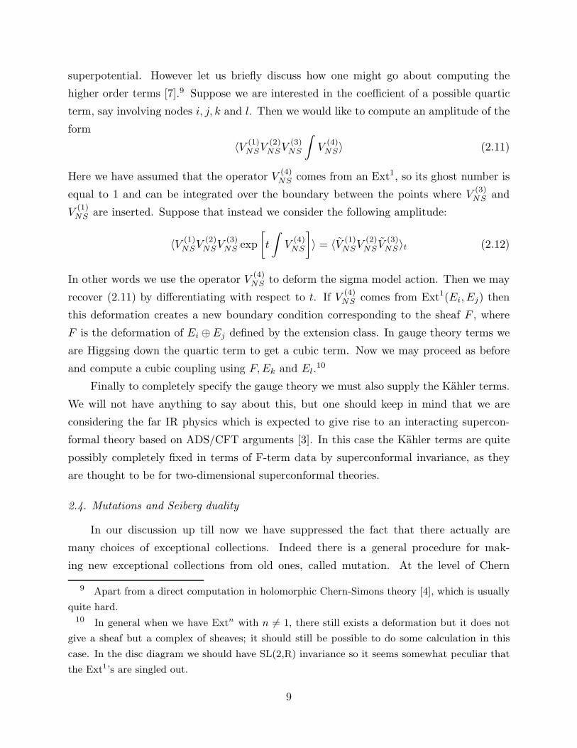
2.4. Mutations and Seiberg duality
In our discussion up till now we have suppressed the fact that there actually are
many choices of exceptional collections. Indeed there is a general procedure for mak-
ing new exceptional collections from old ones, called mutation. At the level of Chern
9 Apart from a direct computation in holomorphic Chern-Simons theory [4], which is usually
quite hard.10 In general when we have Extn with n 6= 1, there still exists a deformation but it does not
give a sheaf but a complex of sheaves; it should still be possible to do some calculation in this
case. In the disc diagram we should have SL(2,R) invariance so it seems somewhat peculiar that
the Ext1’s are singled out.
9
characters this transformation looks very familiar. Given an exceptional collection
. . . , Ei−1, Ei, Ei+1, Ei+2, . . . we can make a new ”left mutated” collection11
. . . , Ei−1, LEiEi+1, Ei, Ei+2, . . . (2.13)
where the Chern character of the new sheaf LEiEi+1 is given by12
ch(LEiEi+1) = ± [ch(Ei+1)− χ(Ei, Ei+1)ch(Ei)] . (2.14)
This looks very similar to (and is in fact mirror to) Picard-Lefschetz monodromy. One
may construct the sheaf LEiEi+1 out of Ei and Ei+1 using certain exact sequences.
~Q
U(N )i
U(N )c Q
Φ
Πi
Πj
Φ
U(N )j U(N )i
cU(N )~
Φ
Πi
Πj
Φ
U(N )jq ~q
ijM
kki jk
ji
kik kj
ji
(A) (B)
fig. 3: (A): Organising the nodes before applying Seiberg duality to node k. (B): Seiberg dual
theory.
For a certain class of mutations the corresponding transformation on the quiver gauge
theory was interpreted as Seiberg duality [7]. Before we delve into this let us first comment
on the abelian factors in the gauge groups. There is an overall factor of U(1) which
completely decouples and then there are relative U(1)’s between the nodes which become
weakly coupled in the infrared. Seiberg duality is a statement about the infrared behaviour
of the non-abelian part of the gauge theory, which can get strongly coupled. So when we
discuss a quiver diagram with U(N) gauge groups we would like to think of the SU(N)
parts as dynamical gauge groups and the U(1)’s as global symmetries, or alternatively
reinstate the U(1)’s as gauge symmetries only at “intermediate” energy scales.
To see which class of mutations we need to look at let us suppose we want to do a
Seiberg duality on node k and organise the quiver so that all the incoming arrows (labelled
by i) are to the left of node k and all the outgoing arrows (labelled by j) to the right of
11 There is also a right shifted version . . . , Ei, REiEi−1, Ei+1, . . ..
12 When we apply this formula in the next section we will deduce the sign using charge
conservation.
10

node k as in fig. 3A. We think SU(Nk) as the colour group which gets strongly coupled
and treat all the other nodes as flavour groups. The total number of flavours is
Nf =∑
i
nikNi =∑
j
nkjNj (2.15)
where the second equality comes from anomaly cancellation as we discussed above. In the
Seiberg dual theory the quarks and anti-quarks Qik, Qkj are replaced by dual quarks
qki, qjk, which means we have to reverse the arrows going into and coming out of node k
in the quiver diagram. We also have to add mesons Mij between the nodes on the left of
k and the nodes on the right of k. In the original theory these mesons are bound states of
the quarks, Mij ∼ QikQkj , but they become fundamental in the dual theory. Finally we
have to replace the original gauge group SU(Nc) = SU(Nk) on node k by the dual gauge
group SU(Nc) = SU(Nf −Nc). If the superpotential for the original theory isW (Q ·Q,Φ)
then the superpotential for the dual theory is
Wdual(q · q,M,Φ) =Worig(M,Φ) + λ Tr(Mqq). (2.16)
Since we are only interested in F-terms, the coupling constant λ is not relevant for our
purposes and can be scaled away.
This transformation can be realised in geometry by doing a mutation by Ek on either
(1) all the sheaves Ei to the left of k or (2) all the sheaves Ej to the right of k [7].13 Let
us illustrate this for the case of P2. Starting with the collection O(−1),Ω1(1),O(0) we
may do a Seiberg duality on node 1 by going to the mutated collection
LO(−1)Ω1(1),O(−1),O(0) = O(−2),O(−1),O(0). (2.17)
Note that in fig. 2B we label the nodes to be consistent with the original quiver fig. 2A,
not according to the order of the exceptional collection. Now for this new collection the
matter fields descend from monomials on P2:
Aizi ∈ Hom(O(−2),O(−1))
Bjzj ∈ Hom(O(−1),O(0))
C∗
ijzizj ∈ Hom(O(−2),O(0)).
(2.18)
13 Some progress has been made towards the understanding of more general mutations [13],
though as we will note in section 3 one doesn’t necessarily expect an arbitrary mutation to give
rise to a good field theory.
11

Here Cij is symmetric in i and j, so there are only six fields, not nine. From the Yoneda
pairings we deduce the superpotential
W = Tr∑
i,j
CijAiBj (2.19)
An easy calculation shows that this agrees with the Seiberg dual of fig. 2A after integrating
out the massive fields, which are irrelevant in the infrared. We create nine new mesons
between nodes 2 and 3 but three of these mesons pair up with fields from the original
theory, leaving six massless fields.
A crucial property of Seiberg duality is that it preserves the moduli space and the
ring of chiral operators of the theory. The moduli space is parametrised by the gauge
invariant operators modulo algebraic relations and relations coming from the superpoten-
tial. We may distinguish between the mesonic operators which are products of ”quarks”
and ”anti-quarks” (i.e. they are gauge invariant because fundamentals are tensored with
anti-fundamentals) and the baryonic operators which are gauge invariant because they
contain an epsilon-tensor. In this article we will investigate the part of the moduli space
parametrised by the mesonic operators. These moduli describe the motion of the branes in
the background geometry. In particular for a single probe brane we expect to recover the
background geometry itself, perhaps with some additional branches if the singularity is not
isolated. The baryonic operators describe partial resolutions of the background (coming
from twisted sector closed strings in the case of orbifolds), and we will make use of them
for comparing the new quiver theories we write down to known quivers in the partially
resolved background.
3. Superpotentials for toric and non-toric Calabi-Yau singularities
In light of the approach sketched in the previous section, the first step in writing
down the quiver theory for branes at a singularity is identifying a suitable exceptional
collection of sheaves at large volume. The Calabi-Yau three-fold singularities we would
like to consider here are complex cones over Del Pezzo surfaces (though we will also make
some comments on the conifold). This just means that we take the equations defining a
Del Pezzo surfaces living in projective space, and regard the same equations as defining
a variety over affine space, which gives a cone over the surface with a singularity at the
origin where the 4-cycle shrinks to zero size.
12

Since the Del Pezzo’s can be obtained from P2 or P1 × P1 by blowing up generic
points, it would be nice to have a simple way to construct exceptional sheaves on the
blow-up from exceptional sheaves on the original variety. This is indeed possible; we
can start for instance with the exceptional collection O(−1),O(0),O(1) on P2, and
let σ denote the map from the nth Del Pezzo to P2 that blows down the exceptional
curves E1 through En. Then an exceptional collection on the nth Del Pezzo is given by
σ∗O(−1), σ∗O(0), σ∗O(1),OE1, . . . ,OEn
[14].14 However this collection is probably not
very useful for constructing quiver theories. The reason is that the OEiare needed to
recover the full moduli space, but since only OEicarries charge for the Ei cycle and such
charges must cancel, it follows that it must appear both as a brane and an anti-brane in
the quiver, thereby at the least breaking supersymmetry.
Other exceptional collections are related by mutation, so we can take the exceptional
collection mentioned above as a starting point and try to get better behaved collections. A
list of some exceptional collections obtained in this way was given in [12]. If we group all
the sheaves that have no relative cohomologies between them together in a single “block”,
then the exceptional collections written down in [12] only consist of three blocks. Such
collections have many useful properties and provide the easiest way to access the Del
Pezzo cases; eg. the matter fields are always given by Ext0’s (corollary 3.4 in [12]) and the
expected superconformal invariance of the gauge theory restricts the superpotential to be
purely cubic. These properties simplify the computations significantly. The allowed three-
block collections were completely determined in [12] by studying a Markov-type equation
αx2 + βy2 + γz2 =√
αβγK2xyz. (3.1)
Here K2 is the degree of the Del Pezzo (which is 9 minus the number of points blown
up), α, β and γ are the numbers of exceptional sheaves in each of the three blocks, and
x, y and z are the ranks of the sheaves in each block (which one can prove to be equal
within each block). This equation is invariant under “block” Seiberg dualities and is a
special case for three-block collections of a Markov equation for more general exceptional
collections which is invariant under arbitrary Seiberg dualities [15]. Equation (3.1) is also
satisfied if one takes x, y and z to be the ranks of the gauge groups within each block,
provided the left hand side of the equation is multiplied by the number N of D3 branes
we are describing. These two possibilities are related by three “block” Seiberg dualities
14 We thank R. Thomas for pointing out this reference.
13
[12]. We would like to mention that (3.1) has been interpreted as a consistency condition
for the vanishing of NSVZ beta-functions in [16].
The nth Del Pezzo has a discrete group of global diffeomorphisms isomorphic to the
exceptional group En. It is known that the induced action of En on the quiver diagram
yields a symmetry of the diagram [12]. It might be interesting to understand what kind of
constraints it puts on the superpotential.
In the following sections we will display our quiver diagrams in “block” notation in
order to avoid cluttering the pictures with arrows. When nodes are grouped together into a
single block, there are no arrows between them. Also, an arrow from one group to another
group signifies an arrow from each node in the first group to each node in the second group.
In the remainder we will also leave out the overall trace of the superpotentials, it being
understood that this has to be added back to get a gauge invariant expression.
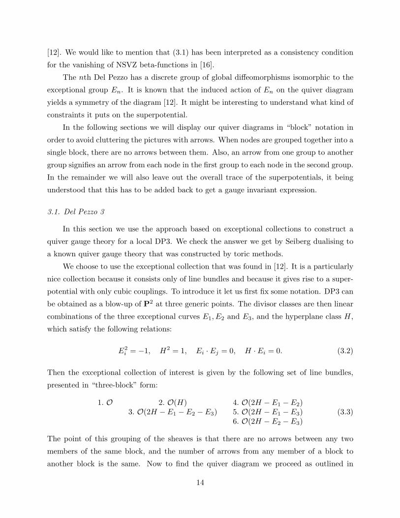
3.1. Del Pezzo 3
In this section we use the approach based on exceptional collections to construct a
quiver gauge theory for a local DP3. We check the answer we get by Seiberg dualising to
a known quiver gauge theory that was constructed by toric methods.
We choose to use the exceptional collection that was found in [12]. It is a particularly
nice collection because it consists only of line bundles and because it gives rise to a super-
potential with only cubic couplings. To introduce it let us first fix some notation. DP3 can
be obtained as a blow-up of P2 at three generic points. The divisor classes are then linear
combinations of the three exceptional curves E1, E2 and E3, and the hyperplane class H,
which satisfy the following relations:
E2i = −1, H2 = 1, Ei ·Ej = 0, H ·Ei = 0. (3.2)
Then the exceptional collection of interest is given by the following set of line bundles,
presented in “three-block” form:
1. O 2. O(H) 4. O(2H − E1 − E2)3. O(2H −E1 −E2 −E3) 5. O(2H − E1 − E3)
6. O(2H − E2 − E3)(3.3)
The point of this grouping of the sheaves is that there are no arrows between any two
members of the same block, and the number of arrows from any member of a block to
another block is the same. Now to find the quiver diagram we proceed as outlined in
14
section 2. For each pair of nodes i and j we need to find the dimensions of Extk(Ei, Ej).
In the case at hand the Ei are line bundles and therefore the Ext’s just reduce to the sheaf
cohomology groups Hk(Ej ⊗E∗i ). The dimensions of these groups are easily computed to
be zero unless k = 0. Let us denote an arbitrary sheaf in the ith block by E(i). Then the
cohomologies are given by:
dim Ext0(E(1), E(2)) = 3, dim Ext0(E(2), E(3)) = 1, dim Ext0(E(1), E(3)) = 4. (3.4)
To find the ranks of the gauge groups, ni, we need to satisfy the equation
∑
i
ni ch(Ei) = ch(Op) (3.5)
where Op is the skyscraper sheaf over a point p on the Del Pezzo. This is just the statement
that the brane configuration has the correct charges of a set of D3 branes filling the
dimensions transverse to the Calabi-Yau, but it will also guarantee that we end up with
an anomaly free theory [7]. In the present case we can take the ni to be
n1, n2, n3, n4, n5, n6 = 1,−2,−2, 1, 1, 1. (3.6)
The effect of the “-2’ on the quiver diagram is that the arrows involving nodes 2 and 3
need to be reversed (because we turned a brane into an anti-brane) and the gauge groups
at these nodes will be U(2N) instead of U(N). The resulting quiver diagram is displayed
below (see the introduction to this section for an explanation of the block notation):
3
14
5
6
1
3
2
4 3 2
14
5
6
1
3
2
(A) (B)
U(N)
U(N)U(2N)
U(2N)
U(N)
U(N)
U(N)U(N)
U(N)
U(N)
U(N)
U(N)
fig. 4: (A) Quiver for the exceptional collection in (3.3). (B) Seiberg dual theory, also known as
”model IV”.
In order to compute the superpotential it is not sufficient to know the dimensions of
H0(Ej⊗E∗i ); we also need to know the generators. These can be represented as polynomials
on the underlying P2.
15
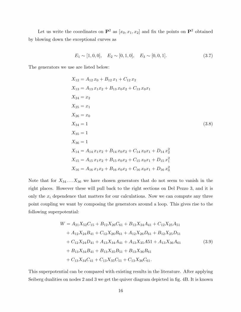
Let us write the coordinates on P2 as [x0, x1, x2] and fix the points on P2 obtained
by blowing down the exceptional curves as
E1 ∼ [1, 0, 0], E2 ∼ [0, 1, 0], E3 ∼ [0, 0, 1]. (3.7)
The generators we use are listed below:
X12 = A12 x0 +B12 x1 + C12 x2
X13 = A13 x1x2 +B13 x0x2 + C13 x0x1
X24 = x2
X25 = x1
X26 = x0
X34 = 1
X35 = 1
X36 = 1
X14 = A14 x1x2 +B14 x0x2 + C14 x0x1 +D14 x22
X15 = A15 x1x2 +B15 x0x2 + C15 x0x1 +D15 x21
X16 = A16 x1x2 +B16 x0x2 + C16 x0x1 +D16 x20
(3.8)
Note that for X34 . . .X36 we have chosen generators that do not seem to vanish in the
right places. However these will pull back to the right sections on Del Pezzo 3, and it is
only the xi dependence that matters for our calculations. Now we can compute any three
point coupling we want by composing the generators around a loop. This gives rise to the
following superpotential:
W = A21X52C15 +B12X26C61 +B12X24A41 + C12X25A51
+ A12X24B41 + C12X26B61 +A12X26D61 +B12X25D51
+ C12X24D41 +A13X34A41 +A13X35A51 +A13X36A61
+B13X34B41 +B13X35B51 +B13X36B61
+ C13X34C41 + C13X35C51 + C13X36C61.
(3.9)
This superpotential can be compared with existing results in the literature. After applying
Seiberg dualities on nodes 2 and 3 we get the quiver diagram depicted in fig. 4B. It is known
16

as model IV in [17,18]. The superpotential obtained through Seiberg duality is
Wdual =−A12A41X24 −A12A51X25 −B12B41X24 − A61B12X26
−B51C12X25 −B61C12X26 + A13B41X34 + A13B51X35
+A41B13X34 +B13B61X36 + A51C13X35 +A61C13X36.
(3.10)
After a relabelling of the nodes and some simple field redefinitions this agrees exactly
with [17,18].
3.2. Del Pezzo 4
In this subsection we analyse the first non-toric example. Its superpotential will again
be completely cubic. The notation will be similar to the previous subsection except that
we add and extra exceptional curve E4 which blows down to
E4 ∼ [1, 1, 1]. (3.11)
Now we proceed with the construction of the quiver. The exceptional collection from [12]
is given by:1. O 2. F 3. O(H)
4. O(2H −E2 −E3 −E4)5. O(2H −E1 −E3 −E4)6. O(2H −E1 −E2 −E4)7. O(2H −E1 −E2 −E3)
(3.12)
Here F is a rank two bundle defined as the unique extension of the line bundles O(H) and
O(2H −∑
iEi):
0 → O(2H −∑
i
Ei) → F → O(H) → 0. (3.13)
The cohomologies for this collection are:
dim Ext0(E(1), E(2)) = 5, dim Ext0(E(2), E(3)) = 1, dim Ext0(E(1), E(3)) = 3. (3.14)
Because of the presence of a rank two bundle our computations differ from those in the
previous subsection. All computations for this case were performed in by embedding the
Del Pezzo in projective space using its anti-canonical embedding and constructing the
sheaves on it in Macaulay2 [19]. Let us make some comments about how this can be done,
since it may be useful for other computations. To get the equations of the Del Pezzo one
picks a linearly independent set of cubic polynomials on P2 which vanish on the points
17
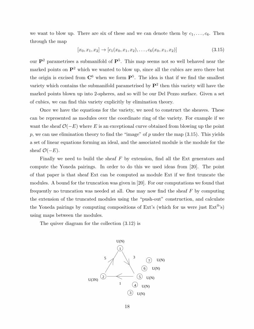
we want to blow up. There are six of these and we can denote them by c1, . . . , c6. Then
through the map
[x0, x1, x2] → [c1(x0, x1, x2), . . . , c6(x0, x1, x2)] (3.15)
our P2 parametrises a submanifold of P5. This map seems not so well behaved near the
marked points on P2 which we wanted to blow up, since all the cubics are zero there but
the origin is excised from C6 when we form P5. The idea is that if we find the smallest
variety which contains the submanifold parametrised by P2 then this variety will have the
marked points blown up into 2-spheres, and so will be our Del Pezzo surface. Given a set
of cubics, we can find this variety explicitly by elimination theory.
Once we have the equations for the variety, we need to construct the sheaves. These
can be represented as modules over the coordinate ring of the variety. For example if we
want the sheaf O(−E) where E is an exceptional curve obtained from blowing up the point
p, we can use elimination theory to find the “image” of p under the map (3.15). This yields
a set of linear equations forming an ideal, and the associated module is the module for the
sheaf O(−E).
Finally we need to build the sheaf F by extension, find all the Ext generators and
compute the Yoneda pairings. In order to do this we used ideas from [20]. The point
of that paper is that sheaf Ext can be computed as module Ext if we first truncate the
modules. A bound for the truncation was given in [20]. For our computations we found that
frequently no truncation was needed at all. One may now find the sheaf F by computing
the extension of the truncated modules using the “push-out” construction, and calculate
the Yoneda pairings by computing compositions of Ext’s (which for us were just Ext0’s)
using maps between the modules.
The quiver diagram for the collection (3.12) is
1
2
5 3
1
6
7
U(N)
U(N)
U(N)
U(N)
U(3N)5
3
4
U(N)
U(N)
18
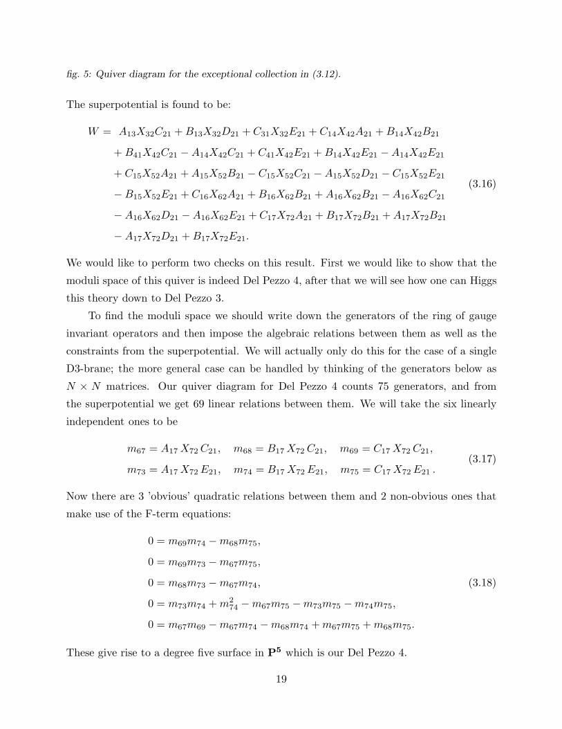
fig. 5: Quiver diagram for the exceptional collection in (3.12).
The superpotential is found to be:
W = A13X32C21 +B13X32D21 + C31X32E21 + C14X42A21 +B14X42B21
+B41X42C21 − A14X42C21 + C41X42E21 +B14X42E21 −A14X42E21
+ C15X52A21 +A15X52B21 − C15X52C21 − A15X52D21 − C15X52E21
−B15X52E21 + C16X62A21 +B16X62B21 + A16X62B21 −A16X62C21
− A16X62D21 − A16X62E21 + C17X72A21 +B17X72B21 +A17X72B21
− A17X72D21 +B17X72E21.
(3.16)
We would like to perform two checks on this result. First we would like to show that the
moduli space of this quiver is indeed Del Pezzo 4, after that we will see how one can Higgs
this theory down to Del Pezzo 3.
To find the moduli space we should write down the generators of the ring of gauge
invariant operators and then impose the algebraic relations between them as well as the
constraints from the superpotential. We will actually only do this for the case of a single
D3-brane; the more general case can be handled by thinking of the generators below as
N × N matrices. Our quiver diagram for Del Pezzo 4 counts 75 generators, and from
the superpotential we get 69 linear relations between them. We will take the six linearly
independent ones to be
m67 = A17X72C21, m68 = B17X72C21, m69 = C17X72C21,
m73 = A17X72E21, m74 = B17X72E21, m75 = C17X72E21 .(3.17)
Now there are 3 ’obvious’ quadratic relations between them and 2 non-obvious ones that
make use of the F-term equations:
0 = m69m74 −m68m75,
0 = m69m73 −m67m75,
0 = m68m73 −m67m74,
0 = m73m74 +m274 −m67m75 −m73m75 −m74m75,
0 = m67m69 −m67m74 −m68m74 +m67m75 +m68m75.
(3.18)
These give rise to a degree five surface in P5 which is our Del Pezzo 4.
19
1
3
1
1
1
3
3
2+7
3 2
14
5
6
1
2+7
3
(A) (B) (C)1
2
34
5
6
72 1
1 1
1
3
U(N)
U(N)
U(N)
U(N)
U(N)
U(2N) U(2N)
U(N)
U(N)
4
5
6
U(N)
U(N) U(N)
U(N)
U(N)
U(N)
U(N)
U(N)
U(N)U(N)
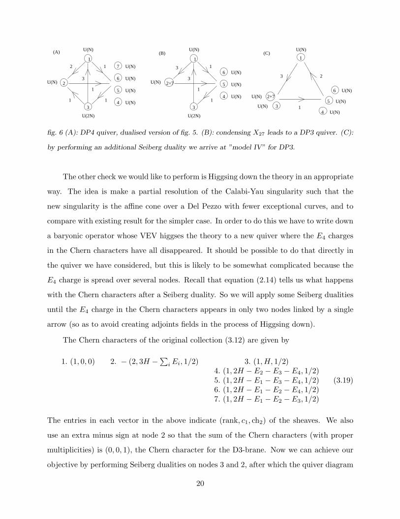
fig. 6 (A): DP4 quiver, dualised version of fig. 5. (B): condensing X27 leads to a DP3 quiver. (C):
by performing an additional Seiberg duality we arrive at ”model IV” for DP3.
The other check we would like to perform is Higgsing down the theory in an appropriate
way. The idea is make a partial resolution of the Calabi-Yau singularity such that the
new singularity is the affine cone over a Del Pezzo with fewer exceptional curves, and to
compare with existing result for the simpler case. In order to do this we have to write down
a baryonic operator whose VEV higgses the theory to a new quiver where the E4 charges
in the Chern characters have all disappeared. It should be possible to do that directly in
the quiver we have considered, but this is likely to be somewhat complicated because the
E4 charge is spread over several nodes. Recall that equation (2.14) tells us what happens
with the Chern characters after a Seiberg duality. So we will apply some Seiberg dualities
until the E4 charge in the Chern characters appears in only two nodes linked by a single
arrow (so as to avoid creating adjoints fields in the process of Higgsing down).
The Chern characters of the original collection (3.12) are given by
1. (1, 0, 0) 2. − (2, 3H −∑
iEi, 1/2) 3. (1, H, 1/2)4. (1, 2H − E2 − E3 − E4, 1/2)5. (1, 2H − E1 − E3 − E4, 1/2)6. (1, 2H − E1 − E2 − E4, 1/2)7. (1, 2H − E1 − E2 − E3, 1/2)
(3.19)
The entries in each vector in the above indicate (rank, c1, ch2) of the sheaves. We also
use an extra minus sign at node 2 so that the sum of the Chern characters (with proper
multiplicities) is (0, 0, 1), the Chern character for the D3-brane. Now we can achieve our
objective by performing Seiberg dualities on nodes 3 and 2, after which the quiver diagram
20
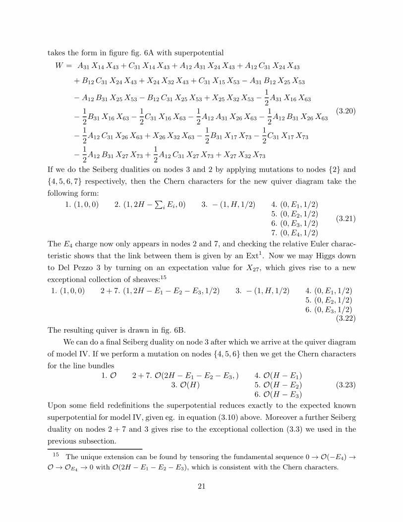
takes the form in figure fig. 6A with superpotential
W = A31X14X43 + C31X14X43 + A12A31X24X43 + A12C31X24X43
+B12C31X24X43 +X24X32X43 + C31X15X53 − A31B12X25X53
− A12B31X25X53 −B12C31X25X53 +X25X32X53 −1
2A31X16X63
−1
2B31X16X63 −
1
2C31X16X63 −
1
2A12A31X26X63 −
1
2A12B31X26X63
−1
2A12C31X26X63 +X26X32X63 −
1
2B31X17X73 −
1
2C31X17X73
−1
2A12B31X27X73 +
1
2A12C31X27X73 +X27X32X73
(3.20)
If we do the Seiberg dualities on nodes 3 and 2 by applying mutations to nodes 2 and
4, 5, 6, 7 respectively, then the Chern characters for the new quiver diagram take the
following form:
1. (1, 0, 0) 2. (1, 2H −∑
iEi, 0) 3. − (1, H, 1/2) 4. (0, E1, 1/2)5. (0, E2, 1/2)6. (0, E3, 1/2)7. (0, E4, 1/2)
(3.21)
The E4 charge now only appears in nodes 2 and 7, and checking the relative Euler charac-
teristic shows that the link between them is given by an Ext1. Now we may Higgs down
to Del Pezzo 3 by turning on an expectation value for X27, which gives rise to a new
exceptional collection of sheaves:15
1. (1, 0, 0) 2 + 7. (1, 2H −E1 −E2 −E3, 1/2) 3. − (1, H, 1/2) 4. (0, E1, 1/2)5. (0, E2, 1/2)6. (0, E3, 1/2)
(3.22)
The resulting quiver is drawn in fig. 6B.
We can do a final Seiberg duality on node 3 after which we arrive at the quiver diagram
of model IV. If we perform a mutation on nodes 4, 5, 6 then we get the Chern characters
for the line bundles1. O 2 + 7. O(2H − E1 − E2 − E3, ) 4. O(H − E1)
3. O(H) 5. O(H − E2)6. O(H − E3)
(3.23)
Upon some field redefinitions the superpotential reduces exactly to the expected known
superpotential for model IV, given eg. in equation (3.10) above. Moreover a further Seiberg
duality on nodes 2 + 7 and 3 gives rise to the exceptional collection (3.3) we used in the
previous subsection.
15 The unique extension can be found by tensoring the fundamental sequence 0 → O(−E4) →
O → OE4→ 0 with O(2H − E1 − E2 − E3), which is consistent with the Chern characters.
21

3.3. Del Pezzo 5
For Del Pezzo surfaces of with more than four exceptional curves we have to deal
with a new phenomenon: these surfaces have a complex structure moduli space. While
our computations are insensitive to the Kahler structure, they definitely do depend on the
complex structure so we expect these moduli to make an appearance in the superpotential.
The appearance of complex structure moduli is easy to understand in the description
of Del Pezzos we have used, as blow-ups of P2. The set of coordinate transformations
preserving the complex structure of P2 is the group PGl(3, C), which has 8 complex pa-
rameters. The complex structure of the Del Pezzos is completely determined by specifying
which points on P2 get blown up. To specify a point on P2 one needs two complex param-
eters. Therefore, the first four marked points can always be fixed at some chosen reference
points, but then we have used up the coordinate transformations and for each additional
point we have a choice of two complex parameters each of which gives rise to a different
complex structure.
With this in mind, for DP5 we add a fifth exceptional curve E5 which blows down
to a point with floating coordinates. For convenience we use projective coordinates to
parametrise this marked point and therefore the complex structure moduli space, E5 ∼
[z0, z1, z2].
The exceptional collection of [12] is given by the following collection of line bundles:
1. O(E5) 3. O(H) 5. O(2H − E1 − E2)2. O(E4) 4. O(2H − E1 − E2 −E3) 6. O(2H − E2 − E3)
7. O(2H − E1 − E3)
8. O(3H −∑5
i=1Ei)
(3.24)
The cohomologies for this collection are:
dim Ext0(E(1), E(2)) = 2, dim Ext0(E(2), E(3)) = 1, dim Ext0(E(1), E(3)) = 3. (3.25)
The quiver diagram for this collection is displayed below:
2
1
3
1 2
3
4
5
6
7
8
U(N) U(N)
U(3N)
U(3N)
U(N)
U(N)
U(N)
U(N)
22
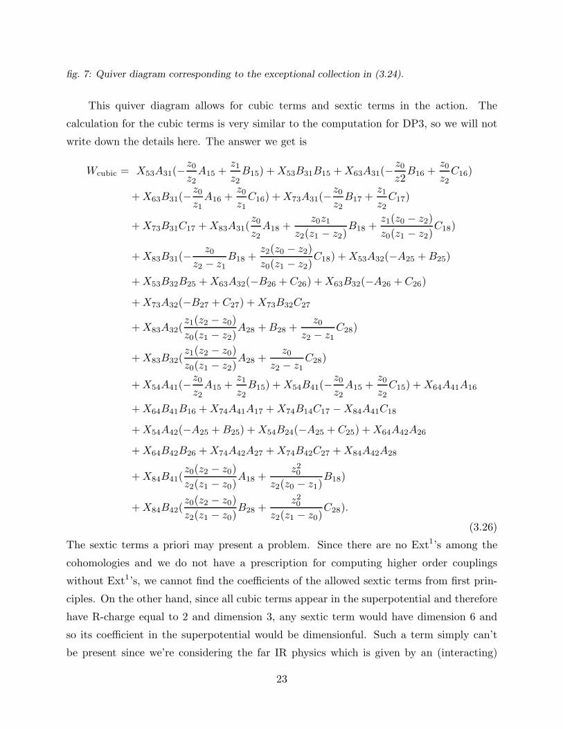
fig. 7: Quiver diagram corresponding to the exceptional collection in (3.24).
This quiver diagram allows for cubic terms and sextic terms in the action. The
calculation for the cubic terms is very similar to the computation for DP3, so we will not
write down the details here. The answer we get is
Wcubic = X53A31(−z0z2A15 +
z1z2B15) +X53B31B15 +X63A31(−
z0z2B16 +
z0z2C16)
+X63B31(−z0z1A16 +
z0z1C16) +X73A31(−
z0z2B17 +
z1z2C17)
+X73B31C17 +X83A31(z0z2A18 +
z0z1z2(z1 − z2)
B18 +z1(z0 − z2)
z0(z1 − z2)C18)
+X83B31(−z0
z2 − z1B18 +
z2(z0 − z2)
z0(z1 − z2)C18) +X53A32(−A25 +B25)
+X53B32B25 +X63A32(−B26 + C26) +X63B32(−A26 + C26)
+X73A32(−B27 + C27) +X73B32C27
+X83A32(z1(z2 − z0)
z0(z1 − z2)A28 +B28 +
z0z2 − z1
C28)
+X83B32(z1(z2 − z0)
z0(z1 − z2)A28 +
z0z2 − z1
C28)
+X54A41(−z0z2A15 +
z1z2B15) +X54B41(−
z0z2A15 +
z0z2C15) +X64A41A16
+X64B41B16 +X74A41A17 +X74B14C17 −X84A41C18
+X54A42(−A25 +B25) +X54B24(−A25 + C25) +X64A42A26
+X64B42B26 +X74A42A27 +X74B42C27 +X84A42A28
+X84B41(z0(z2 − z0)
z2(z1 − z0)A18 +
z20z2(z0 − z1)
B18)
+X84B42(z0(z2 − z0)
z2(z1 − z0)B28 +
z20z2(z1 − z0)
C28).
(3.26)
The sextic terms a priori may present a problem. Since there are no Ext1’s among the
cohomologies and we do not have a prescription for computing higher order couplings
without Ext1’s, we cannot find the coefficients of the allowed sextic terms from first prin-
ciples. On the other hand, since all cubic terms appear in the superpotential and therefore
have R-charge equal to 2 and dimension 3, any sextic term would have dimension 6 and
so its coefficient in the superpotential would be dimensionful. Such a term simply can’t
be present since we’re considering the far IR physics which is given by an (interacting)
23
scale-invariant theory. One may also take a limit in which the generic Del Pezzo becomes
a toric surface and compare with toric computations which can be done independently. In
this limit one finds only cubic terms. So we conclude that the cubic terms provide the full
answer.
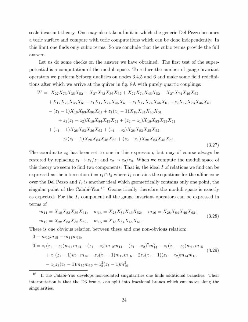
Let us do some checks on the answer we have obtained. The first test of the super-
potential is a computation of the moduli space. To reduce the number of gauge invariant
operators we perform Seiberg dualities on nodes 3,4,5 and 6 and make some field redefini-
tions after which we arrive at the quiver in fig. 8A with purely quartic couplings:
W = X27X73X35X52 +X27X73X36X62 +X27X74X45X52 +X27X74X46X62
+X17X73X36X61 +z1X17X74X45X51 +z1X17X74X46X61 +z2X17X73X35X51
− (z1 − 1)X18X83X36X61 + z1(z1 − 1)X18X84X46X61
+ z1(z1 − z2)X18X84X45X51 + (z2 − z1)X18X83X35X51
+ (z1 − 1)X28X83X36X62 + (z1 − z2)X28X83X35X52
− z2(z1 − 1)X28X84X46X62 + (z2 − z1)X28X84X45X52.
(3.27)
The coordinate z0 has been set to one in this expression, but may of course always be
restored by replacing z1 → z1/z0 and z2 → z2/z0. When we compute the moduli space of
this theory we seem to find two components. That is, the ideal I of relations we find can be
expressed as the intersection I = I1∩I2 where I1 contains the equations for the affine cone
over the Del Pezzo and I2 is another ideal which geometrically contains only one point, the
singular point of the Calabi-Yau.16 Geometrically therefore the moduli space is exactly
as expected. For the I1 component all the gauge invariant operators can be expressed in
terms of
m11 = X18X83X36X61, m14 = X28X84X45X52, m16 = X28X84X46X62,
m12 = X28X83X36X62, m15 = X18X84X46X61.(3.28)
There is one obvious relation between these and one non-obvious relation:
0 = m12m15 −m11m16,
0 = z1(z1 − z2)m11m14 − (z1 − z2)m12m14 − (z1 − z2)2m2
14 − z1(z1 − z2)m14m15
+ z1(z1 − 1)m11m16 − z2(z1 − 1)m12m16 − 2z2(z1 − 1)(z1 − z2)m14m16
− z1z2(z1 − 1)m15m16 + z22(z1 − 1)m216.
(3.29)
16 If the Calabi-Yau develops non-isolated singularities one finds additional branches. Their
interpretation is that the D3 branes can split into fractional branes which can move along the
singularities.
24
It would be interesting to check if this Del Pezzo has the expected complex structure.
7
1+2+8
34
1
1
1+8
11
1
1
1(B)
1 1
34
2
1
(C)
1
2
1
11
1
12
34
8
7
(A)
2
5
6
5
6
U(N) U(N)
U(N)
U(N)
U(N) U(N)
U(N)
U(N)
5
6
7
U(N)
U(N)
U(N)
U(N) U(N) U(N) U(N)
U(N)
U(N)
U(N)
U(N)
U(N)
U(N)
fig. 8 (A): Quiver obtained by dualising fig. 7. (B): Giving a VEV to X18 in (A), which results in
a quiver for Del Pezzo 4. (C): Further condensing X28 gives rise to “model III” for Del Pezzo 3.
Another possible way of testing the superpotentials is by Higgsing down to known Del
Pezzo’s as we did for Del Pezzo 4. The simplest way to do that in the present case is by
giving an expectation value to X18 in the quiver of fig. 8A, after which we get the quiver
theory in fig. 8B without having to do any integrating out. One can straightforwardly
check that the moduli space of this quiver is exactly Del Pezzo 4. One may Higgs it down
further to Del Pezzo 3 by condensing X28. This quiver is known as “model III” [17,18], and
the superpotential we get coincides with the known superpotential after field redefinitions.
The quiver theory in fig. 8B is related to the Del Pezzo 4 quiver we found in the
previous subsection. Namely we can start with fig. 5 and apply Seiberg dualities on nodes
2,3,4,2,5.
Finally one can take a limit in which some of the marked points approach each other.
In such a limit the shrinking 4-cycle may cease to have a positive curvature anti-canonical
bundle and so would therefore no longer be a Del Pezzo surface, but one may obtain cones
over toric surfaces in such limits or sometimes even orbifolds. For Del Pezzo 5 there is a
limit in which the Calabi-Yau turns into the Z2 ×Z2 orbifold of the conifold, and another
in which it becomes a partial toric resolution of the orbifold singularity C3/Z3 × Z3 and
hence we may compare with known answers in the literature. We have not carried out the
details because the field rescalings are rather involved, but it should be possible to check
this.
25

3.4. Del Pezzo 6
For Del Pezzo 6 two three-block models were given in [12]. We can compute the cubic
couplings in either without too much difficulty, but we will stick to the collection of line
bundles because it is easier to get the dependence on complex structure moduli that way.
We blow up a sixth point on P2 with floating coordinates
E6 ∼ [w0, w1, w2]. (3.30)
The exceptional sheaves of the first collection in [12], which we might call “ model 6.1”,
are:1. O(E4) 4. O(H −E1) 7. O(2H − E1 − E2 − E3)2. O(E5) 5. O(H −E2) 8. O(H)
3. O(E6) 6. O(H −E3) 9. O(3H −∑6
i=1Ei)
(3.31)
with cohomologies given by
dim Ext0(E(1), E(2)) = 1, dim Ext0(E(2), E(3)) = 1, dim Ext0(E(1), E(3)) = 2. (3.32)
The quiver for this collection is displayed in fig. 9A.
123
4
5
6
8
9
1 2
1 7
(B)(A) U(N) U(N)
U(N)
U(N)
U(2N)
U(2N)
123
4
5
6
11
7
8
9
1
U(N)
U(N)
U(N)
U(N) U(N) U(N)
U(N)
U(N)
U(N)
U(N)
U(N)
U(2N)
fig. 9 (A): Quiver diagram corresponding to the exceptional collection in (3.31). (B): Seiberg dual
quiver; also the quiver diagram for the orbifold C3/Z3 × Z3. Notice the similarity between these
two quivers and the P2 quivers in fig. 2.
Before writing down the superpotential let us introduce the following shorthand no-
tation:f1 = (z1 − z0)z2w
20 + (z20 − z1z2)w0w2 + z0(z2 − z0)w1w2
f2 = z0(z1 − z2)w1w2 + (z0 − z1)z2w0w1 + (z2 − z0)z1w0w2
f3 = −z1(z2 − z1)w0w2 − (z0 − z1)z2w21 − (z21 − z0z2)w1w2.
(3.33)
26

The cubic terms in the superpotential for model 6.1 are
W = (−a71 + b71) x14 x47 + x24 x47
(
b72 −a72 z1z2
)
+
(
b73 −a73w1
w2
)
x34 x47
+ a81 x14 x48 + a82 x24 x48 + a83 x34 x48
+
(
b91 +a91 f1f2
)
x14 x49 +
(
b92 +a92 f1f2
)
x24 x49 +
(
b93 +a93 f1f2
)
x34 x49
+ b71 x15 x57 + b72 x25 x57 + b73 x35 x57
+ b81 x15 x58 + b82 x25 x58 + b83 x35 x58
+
(
b91 +a91 f2f3
)
x15 x59 +
(
b92 +a92 f2f3
)
x25 x59 +
(
b93 +a93 f2f3
)
x35 x59
+ a71 x16 x67 + a72 x26 x67 + a73 x36 x67
+ (−a81 + b81) x16 x68 + x26 x68
(
b82 −a82 z0z1
)
+
(
b83 −a83w0
w1
)
x36 x68
+ (−a91 + b91) x16 x69 +
(
b93 −a93w0
w1
)
x36 x69 + x26 x69
(
b92 −a92 z0z1
)
(3.34)
As for Del Pezzo 5 we expect this to be the full answer.
In order to do the moduli space computation we go to a new quiver by Seiberg dualities
on nodes 4,5,6, after which we get fig. 9B with superpotential
W = X17(X41X74 −X51X75 +X61X76)
+X18(X41X84 −X51X85 +X61X86)
+X19((−f22 − f2f3)X41X94 + (f1f3 + f2f3)X51X95 + (f2
2 − f1f3)X61X96)
+X27(X62X76z1 +X42X74z2 −X52X75z2)
+X28(X42X84z0 −X52X85z1 +X62X86z1)
+X29((−f2f3z0 − f22 z1)X42X94 + (f2f3z0 + f1f3z1)X52X95)
+X29(z1(f22 − f1f3)X62X96) +X37(w2(X43X74 −X53X75) + w1X63X76)
+X38(w0X43X84 − w1X53X85 + w1X63X86) +X39((−f2f3w0− f22w1)X43X94)
+X39((f2f3w0+ f1f3w1)X53X95 + w1(f22 − f1f3)X63X96)
(3.35)
When we calculate the ideal of relations we find, just as for Del Pezzo 5, that it can be
expressed as I = I1∩I2 where I1 gives a cubic relation in four variables and I2 only contains
the origin of moduli space geometrically. As before to get the locus of the moduli space
one should take the radical of I, leaving us only with a cubic equation. We were not able
27
to get a general expression involving the complex structure parameters as in (3.29), but
we can find the cubic equation for any given complex structure. The 207 gauge invariant
operators can all be solved for in terms of
p23 = X29X95X52, p24 = X39X95X53, p26 = X29X96X62, p27 = X39X96X63. (3.36)
If for example the complex structure is given by [z0, z1, z2] = [1, 3, 5] and [w0, w1, w2] =
[1, 2,−2], we get
0 = p23 p24 p26 +4
43p224 p26 +
105
731p24 p
226 +
5
43p223 p27 +
20
43p23 p24 p27
−825
731p23 p26 p27 −
10
731p24 p26 p27 −
350
731p23 p
227.
(3.37)
We recognise the well-known realisation of Del Pezzo 6 as a degree 3 surface in P3.
1+2+3+9
7
1
1
31
3
(A) (B)123
7
8
9
1
1
1
1
U(N)
U(N)
4
5
6
U(2N)
U(N)
U(N)
U(N) 4
5
6
8
U(2N)
U(N)
U(N)
U(N)
U(N)
U(N) U(N) U(N)
U(N)
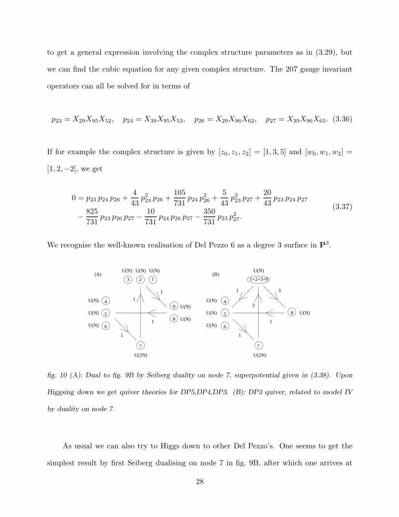
fig. 10 (A): Dual to fig. 9B by Seiberg duality on node 7, superpotential given in (3.38). Upon
Higgsing down we get quiver theories for DP5,DP4,DP3. (B): DP3 quiver, related to model IV
by duality on node 7.
As usual we can also try to Higgs down to other Del Pezzo’s. One seems to get the
simplest result by first Seiberg dualising on node 7 in fig. 9B, after which one arrives at
28

fig. 10A with superpotential
W = −X18X47X71X84 −w0
w2X38X47X73X84 −X18X57X71X85
−w1
w2X38X57X73X85 −X18X67X71X86 −X28X67X72X86 −X38X67X73X86
+ f22 X19X47X71X94 + f2 f3X19X47X71X94 +
f2 f3w0
w2X39X47X73X94
+f22 w1
w2X39X47X73X94 + f1 f3X19X57X71X95 + f2 f3X19X57X71X95
+f2 f3w0
w2X39X57X73X95 +
f1 f3w1
w2X39X57X73X95 − f2
2 X19X67X71X96
+ f1 f3X19X67X71X96 − f22 X29X67X72X96 + f1 f3X29X67X72X96
− f22 X39X67X73X96 + f1 f3X39X67X73X96 −
z0z2X28X47X72X84
+f2 f3 z0z2
X29X47X72X94 +f2 f3 z0z2
X29X57X72X95 −z1z2X28 X57X72X85
+f22 z1z2
X29X47X72X94 +f1 f3 z1z2
X29X57X72X95
(3.38)
One can arrange the links X39, X29 and X19 to correspond to Ext1’s, and by successively
condensing them one should get exceptional collections, quiver diagrams and superpoten-
tials for Del Pezzo 5,4, and 3 respectively. There is no integrating out involved so this
is very simple. By doing an additional Seiberg duality on node 7 in fig. 10B, we get the
quiver diagram for model IV yet again and we have checked that one recovers the known
superpotential for the quiver after going through this sequence all the way.
The C3/Z3 × Z3 orbifold is a limit of Del Pezzo 6 and its quiver diagram is given
by fig. 9B. The orbifold superpotential is completely cubic and our superpotential should
reproduce this in the appropriate limit. This looks promising but we haven’t been able to
check it precisely due to the large number of allowed field rescalings.
3.5. Simple quiver diagrams for the remaining Del Pezzo’s
Let us list some quiver diagrams that can be deduced from the collections in [12] for
Del Pezzo surfaces of degree 1 and 2.17 We haven’t yet computed the superpotentials for
these quivers but they should give rise to cubic couplings only.
17 Quiver diagrams for low degree Del Pezzo’s have been proposed before (see the fourth
reference in [18]) but they were found to have some problems; for degree 3 this was found by
F. Cachazo and the author, and for degrees 1 and 2 in [21]
29

1
2
9
10
3
4
5
6
7
8
U(2N)
U(6N)
U(N)
U(N)
U(N)
U(N)
U(N)
U(N)
U(N)
U(N)4
1
3
12
3
4
5
10
6 7
8
9
U(N)
U(N)
U(N)
U(N)U(N)
U(N)
U(N)
U(2N) U(2N)
1 1
1U(N)
3
4
5
6
8
9
2
10
7
1
U(N)
U(N)
U(N)
U(N)
U(N)
U(N)
U(N)
U(3N)
U(N)
U(N)
1
1
2
(A) (B) (C)
fig. 11: Three quivers diagrams for the degree 2 Del Pezzo. All these should have a cubic super-
potential. (A): Type (7.1). (B): Type (7.2). (C): Type (7.3).
Let us start with collection (7.1) in [12]. The Chern characters are computed to be:
1. (2,−2H +∑
iEi,−3/2) 2. − (2, H,−1/2) 3. (1, 3H −∑
iEi, 1)4. (1, H −E1, 0)5. (1, H −E2, 0)6. (1, H −E3, 0)7. (1, H −E4, 0)8. (1, H −E5, 0)9. (1, H −E6, 0)10. (1, H −E7, 0)
(3.39)
The corresponding quiver diagram is drawn in figure fig. 11A. The quiver can be simplified
by dualising node 2, which reduces the gauge group to U(2N).
It is instructive to see how one may get the other allowed types of three-block quivers
through Seiberg duality. In principle we could get them from the collections in [12], however
computation of the cohomologies for the remaining collections reveals that some of them
fail to be exceptional. In these cases one may write down a valid set by following the Chern
characters through Seiberg dualities, as we discussed in detail for the degree 5 Del Pezzo.
To get a new type of three-block quiver we can start with (3.39) and apply Seiberg
dualities on nodes 2, 3, 4, 5, 6, 2 after which one arrives at the quiver depicted in fig. 11B.
This quiver belongs to the class of three-block collections called (7.2) in [12]. Starting
with (3.39) and applying dualities on nodes 2, 3, 4, 5, 1, 2 results in the quiver in fig. 11C,
which is of type (7.3).
Similarly we can get simple quiver diagrams for the degree 1 Del Pezzo. Collection
(8.1) in [12] appears to be invalid so we skip to collection (8.2). The Chern characters are
30

found to be
1. (4,∑4i=1Ei,−5/2) 2. − (2, H,−1/2) 4. (1, H −E1, 0)
3. − (2, 2H −∑3i=1,−1/2) 5. (1, H −E2, 0)
6. (1, H −E3, 0)7. (1, 3H −
∑
iEi + E8, 1)8. (1, 3H −
∑
iEi + E7, 1)9. (1, 3H −
∑
iEi + E6, 1)10. (1, 3H −
∑
iEi + E5, 1)11. (1, 3H −
∑
iEi + E4, 1)(3.40)
1
U(N)
U(N)
U(N)
U(N)
U(N)
U(N)
U(N)
U(N)
1
2
3
6
8
10
11
9
7
5
4
2
U(4N)
1
U(2N)
U(2N)
(B)
1
U(N)
U(N)
U(N)
U(N)
U(N)
U(N)
U(N)
U(N)
1
3
2
3
6
8
10
11
9
7
5
4
U(6N)
U(6N)
2
U(4N)(A)
fig. 12: Quivers diagrams for the degree 1 Del Pezzo. All these should have a cubic superpotential.
(A): Collection (3.40), type (8.2). (B): Seiberg dual.
The corresponding quiver diagram is shown in fig. 12A. A simpler quiver may be
obtained through Seiberg duality on nodes 2 and 3, drawn in fig. 12B. From here we
may obtain the other types of three-block quivers through Seiberg duality. Type (8.1)
can be recovered by dualising 4, 1, 2, 3, type (8.3) by dualising 4, 5, 1, and type (8.4)
by dualising 4, 5, 6, 1, 4, 5, 6. The resulting diagrams are given in fig. 13A, fig. 13B and
fig. 13C respectively.
1
1
(A)
4
6
8
11
2
10
9
7
3
5
1 1
U(3N)
U(3N)
U(N)
U(N)
U(N)
U(N)
U(N)
U(N)
U(N)
U(N)
U(N)
U(N)
U(N)
U(N)
1
1
(B)
1 2 3
4
10
11
9
8
7
6
5
U(2N) U(2N) U(2N)
U(3N)
U(3N)
U(N)
U(N)
U(N)
1
U(2N)
U(2N)
U(2N)
U(2N)
U(2N) U(N)
U(N)U(N)
U(N)
U(N)
1
2
4
5
6
9
10
7
8
11
3
1
U(5N)
1 2
(C)
fig. 13: Other quivers diagrams for the degree 1 Del Pezzo with cubic superpotential. (A): Type
(8.1). (B): Type (8.3). (C): Type (8.4).
31
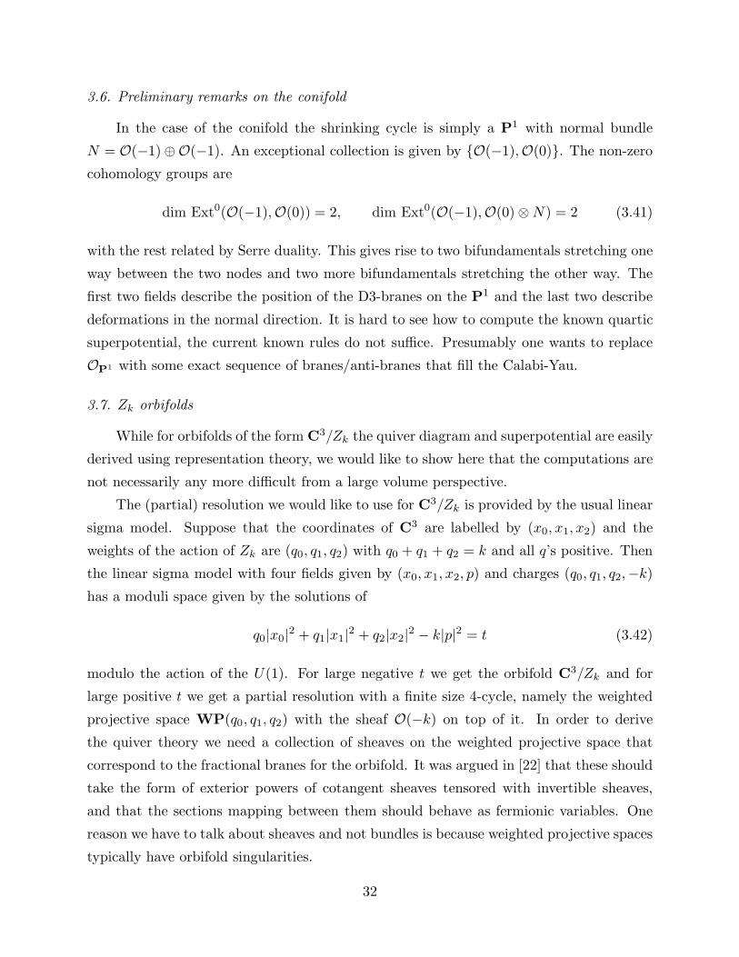
3.6. Preliminary remarks on the conifold
In the case of the conifold the shrinking cycle is simply a P1 with normal bundle
N = O(−1)⊕O(−1). An exceptional collection is given by O(−1),O(0). The non-zero
cohomology groups are
dim Ext0(O(−1),O(0)) = 2, dim Ext0(O(−1),O(0)⊗N) = 2 (3.41)
with the rest related by Serre duality. This gives rise to two bifundamentals stretching one
way between the two nodes and two more bifundamentals stretching the other way. The
first two fields describe the position of the D3-branes on the P1 and the last two describe
deformations in the normal direction. It is hard to see how to compute the known quartic
superpotential, the current known rules do not suffice. Presumably one wants to replace
OP1 with some exact sequence of branes/anti-branes that fill the Calabi-Yau.
3.7. Zk orbifolds
While for orbifolds of the form C3/Zk the quiver diagram and superpotential are easily
derived using representation theory, we would like to show here that the computations are
not necessarily any more difficult from a large volume perspective.
The (partial) resolution we would like to use for C3/Zk is provided by the usual linear
sigma model. Suppose that the coordinates of C3 are labelled by (x0, x1, x2) and the
weights of the action of Zk are (q0, q1, q2) with q0 + q1 + q2 = k and all q’s positive. Then
the linear sigma model with four fields given by (x0, x1, x2, p) and charges (q0, q1, q2,−k)
has a moduli space given by the solutions of
q0|x0|2 + q1|x1|
2 + q2|x2|2 − k|p|2 = t (3.42)
modulo the action of the U(1). For large negative t we get the orbifold C3/Zk and for
large positive t we get a partial resolution with a finite size 4-cycle, namely the weighted
projective space WP(q0, q1, q2) with the sheaf O(−k) on top of it. In order to derive
the quiver theory we need a collection of sheaves on the weighted projective space that
correspond to the fractional branes for the orbifold. It was argued in [22] that these should
take the form of exterior powers of cotangent sheaves tensored with invertible sheaves,
and that the sections mapping between them should behave as fermionic variables. One
reason we have to talk about sheaves and not bundles is because weighted projective spaces
typically have orbifold singularities.
32
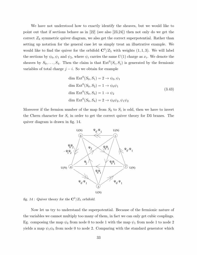
We have not understood how to exactly identify the sheaves, but we would like to
point out that if sections behave as in [22] (see also [23,24]) then not only do we get the
correct Zk symmetric quiver diagram, we also get the correct superpotential. Rather than
setting up notation for the general case let us simply treat an illustrative example. We
would like to find the quiver for the orbifold C3/Z5 with weights (1, 1, 3). We will label
the sections by ψ0, ψ1 and ψ2, where ψi carries the same U(1) charge as xi. We denote the
sheaves by S0, . . . , S4. Then the claim is that Ext0(Si, Sj) is generated by the fermionic
variables of total charge j − i. So we obtain for example
dim Ext0(S0, S1) = 2 → ψ0, ψ1
dim Ext0(S0, S2) = 1 → ψ0ψ1
dim Ext0(S0, S3) = 1 → ψ2
dim Ext0(S0, S4) = 2 → ψ0ψ2, ψ1ψ2
(3.43)
Moreover if the fermion number of the map from S0 to Si is odd, then we have to invert
the Chern character for Si in order to get the correct quiver theory for D3 branes. The
quiver diagram is drawn in fig. 14.
ψ , ψ
ψ2
ψ ψ10
ψ ψ1
ψ2
ψ , ψ0 1
ψ , ψ
0
ψ ψ0 1
0 1
2
3
4
U(N)
U(N)U(N)
U(N) U(N)
ψ , ψ0 1ψ ψ
1 2
0 2ψ ψ
_
0 1 0 1
fig. 14 : Quiver theory for the C3/Z5 orbifold.
Now let us try to understand the superpotential. Because of the fermionic nature of
the variables we cannot multiply too many of them, in fact we can only get cubic couplings.
Eg. composing the map ψ0 from node 0 to node 1 with the map ψ1 from node 1 to node 2
yields a map ψ1ψ0 from node 0 to node 2. Comparing with the standard generator which
33
we chose to be ψ0ψ1, we see that we get a −1 as the coefficient of the corresponding cubic
term in the superpotential. Continuing in this way we find that
W = (Y01X12 −X01Y12)Z20 + (Y12X23 −X12Y23)Z31 + (Y23X34 −X23Y34)Z42
+ (Y34X40 −X34Y40)Z03 + (Y40X01 −X40Y01)Z14
(3.44)
which is just the usual answer obtained by projecting the superpotential of N = 4 Yang-
Mills theory. The linear sigma model with charges (2, 2, 1) provides a different partial
resolution of the same orbifold, but leads to the same quiver diagram and superpotential
up to a permutation of the nodes.
Acknowledgements:
First and foremost I would like to thank F. Cachazo, S. Katz and C. Vafa for initial
collaboration and many valuable discussions. In addition I would like to thank the or-
ganisers of the Workshop on Stacks and Computation at Urbana-Champaign, June 2002,
H. Schenck and M. Stillman for introduction to and help with Macaulay2 at this work-
shop, Y.-H. He for discussions on toric duality and “chilling” (i.e. doing M2 assignments
at 2 a.m.), and the University of Amsterdam, the Centre for Mathematical Sciences at
Zhejiang University, and the Morningside Centre in Beijing for hospitality. This work was
supported in part by grant NSF-PHY/98-02709.
34

References
[1] J. Polchinski, “Dirichlet-Branes and Ramond-Ramond Charges,” Phys. Rev. Lett. 75,
4724 (1995) [arXiv:hep-th/9510017].
[2] M. R. Douglas and G. W. Moore, “D-branes, Quivers, and ALE Instantons,”
arXiv:hep-th/9603167.
[3] D. R. Morrison and M. R. Plesser, “Non-spherical horizons. I,” Adv. Theor. Math.
Phys. 3, 1 (1999) [arXiv:hep-th/9810201].
[4] E. Witten, “Chern-Simons gauge theory as a string theory,” Prog. Math. 133, 637
(1995) [arXiv:hep-th/9207094].
[5] M. Bershadsky, S. Cecotti, H. Ooguri and C. Vafa, “Kodaira-Spencer theory of gravity
and exact results for quantum string amplitudes,” Commun. Math. Phys. 165, 311
(1994) [arXiv:hep-th/9309140].
[6] K. Hori, A. Iqbal and C. Vafa, “D-branes and mirror symmetry,” arXiv:hep-
th/0005247.
[7] F. Cachazo, B. Fiol, K. A. Intriligator, S. Katz and C. Vafa, “A geometric unification
of dualities,” Nucl. Phys. B 628, 3 (2002) [arXiv:hep-th/0110028].
[8] M. R. Douglas, “D-branes, categories and N = 1 supersymmetry,” J. Math. Phys. 42,
2818 (2001) [arXiv:hep-th/0011017].
I. Brunner, M. R. Douglas, A. E. Lawrence and C. Romelsberger, “D-branes on the
quintic,” JHEP 0008, 015 (2000) [arXiv:hep-th/9906200].
D. Berenstein and M. R. Douglas, “Seiberg duality for quiver gauge theories,”
arXiv:hep-th/0207027.
[9] M. R. Douglas, B. Fiol and C. Romelsberger, “The spectrum of BPS branes on a
noncompact Calabi-Yau,” arXiv:hep-th/0003263.
[10] S. Katz and E. Sharpe, “D-branes, open string vertex operators, and Ext groups,”
arXiv:hep-th/0208104.
[11] L. E. Ibanez, R. Rabadan and A. M. Uranga, Nucl. Phys. B 542, 112 (1999)
[arXiv:hep-th/9808139].
[12] Boris V. Karpov, Dmitri Yu. Nogin, “Three-block exceptional collections over Del
Pezzo surfaces,” Izvestiya Math ??? [arXiv:alg-geom/9703027].
[13] F. Cachazo, S. Katz, M. Rocek, C. Vafa, M. Wijnholt.
[14] A. Bondal and D. Orlov, “Semiorthogonal decomposition for algebraic varieties,”
arXiv:alg-geom/9506012.
[15] B. Feng, A. Hanany, Y. H. He and A. Iqbal, “Quiver theories, soliton spectra and
Picard-Lefschetz transformations,” JHEP 0302, 056 (2003) [arXiv:hep-th/0206152].
[16] C. P. Herzog and J. Walcher, “Dibaryons from exceptional collections,” JHEP 0309,
060 (2003) [arXiv:hep-th/0306298].
35
[17] C. E. Beasley and M. R. Plesser, “Toric duality is Seiberg duality,” JHEP 0112, 001
(2001) [arXiv:hep-th/0109053].
[18] B. Feng, A. Hanany, Y. H. He and A. M. Uranga, “Toric duality as Seiberg duality
and brane diamonds,” JHEP 0112, 035 (2001) [arXiv:hep-th/0109063].
B. Feng, A. Hanany and Y. H. He, “Phase structure of D-brane gauge theories and
toric duality,” JHEP 0108, 040 (2001) [arXiv:hep-th/0104259].
B. Feng, S. Franco, A. Hanany and Y. H. He, “Unhiggsing the del Pezzo,” arXiv:hep-
th/0209228.
A. Hanany and A. Iqbal, “Quiver theories from D6-branes via mirror symmetry,”
JHEP 0204, 009 (2002) [arXiv:hep-th/0108137].
[19] Daniel R. Grayson and Michael E. Stillman, “Macaulay 2, a software system for re-
search in algebraic geometry,” Available at http://www.math.uiuc.edu/Macaulay2/
[20] Gregory G. Smith, “Computing Global Extension Modules for Coherent Sheaves
on a Projective Scheme,” Journal of Symbolic Computation 29 (2000) 729-746
[arXiv:math.AG/9807170].
[21] C. P. Herzog and J. McKernan, “Dibaryon spectroscopy,” JHEP 0308, 054 (2003)
[arXiv:hep-th/0305048].
[22] P. Mayr, “Phases of supersymmetric D-branes on Kaehler manifolds and the McKay
correspondence,” JHEP 0101, 018 (2001) [arXiv:hep-th/0010223].
[23] S. Govindarajan and T. Jayaraman, “D-branes, exceptional sheaves and quivers
on Calabi-Yau manifolds: From Mukai to McKay,” Nucl. Phys. B 600, 457 (2001)
[arXiv:hep-th/0010196].
[24] A. Tomasiello, “D-branes on Calabi-Yau manifolds and helices,” JHEP 0102, 008
(2001) [arXiv:hep-th/0010217].
36
Recommended


![arXiv:physics/9711021v2 [physics.data-an] 16 Dec 1999 · arXiv:physics/9711021v2 [physics.data-an] 16 Dec 1999 HUTP-97/A096 ... (February 2, 2008) Abstract We give ... In this paper,](https://img.pdfslide.us/doc/110x75/5ade914e7f8b9ae1408e8817/arxivphysics9711021v2-16-dec-1999-physics9711021v2-16-dec-1999-hutp-97a096.jpg)


![arXiv:cond-mat/9809199v1 [cond-mat.soft] 14 Sep 1998 · 2018-08-13 · arXiv:cond-mat/9809199v1 [cond-mat.soft] 14 Sep 1998 HUTP-98/A068 hep-th/9809199 QuantumFieldTheoryofTreasuryBonds](https://img.pdfslide.us/doc/110x75/5f93b0c91eaaf811e10a50c8/arxivcond-mat9809199v1-cond-matsoft-14-sep-1998-2018-08-13-arxivcond-mat9809199v1.jpg)