Are you being
blinded by statistics?


The structure of the retinal nerve fibre layer

A greyscale showing the visual field for a glaucomatous eye
Blind Spot
Defect
The principle of filtering – reduce the noise, but preserve the
information of interest

Effect of the noise-reduction filter on the greyscale
Noise
• Currently measured by test-retest variability
• Currently assumed to be normally distributed

The Principle:
Noise = Raw - Filtered
Why this method?
Current estimates of the noise are based on test-retest variability.
• This greatly reduces the amount of data available
• It imposes more cost and inconvenience on the clinician and patient
• It is actually estimating double the noise!

Analysing the noise
• Calculate the noise at each point of each visual field
• Separate out the noise estimates according to the filtered sensitivity (in 0.5dB bands)
• Estimate the empirical distribution characteristics at each sensitivity
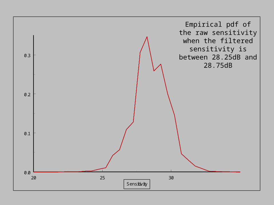
20 25 30Sensitivity
0.0
0.1
0.2
0.3
Empirical pdf of the raw sensitivity when the filtered sensitivity is
between 28.25dB and 28.75dB
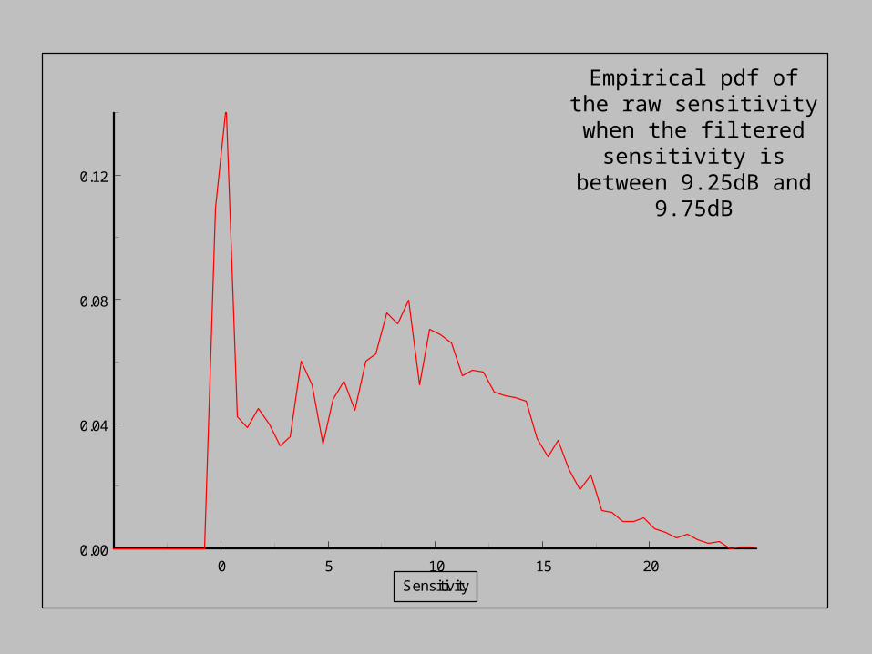
Empirical pdf of the raw sensitivity when the filtered sensitivity is between 9.25dB and
9.75dB
0 5 10 15 20Sensitivity
0.00
0.04
0.08
0.12

How does the noise change?
As the sensitivity decreases;
• The mean noise changes
• The variance increases exponentially
• The negative skewness increases
• The censoring at zero becomes apparent

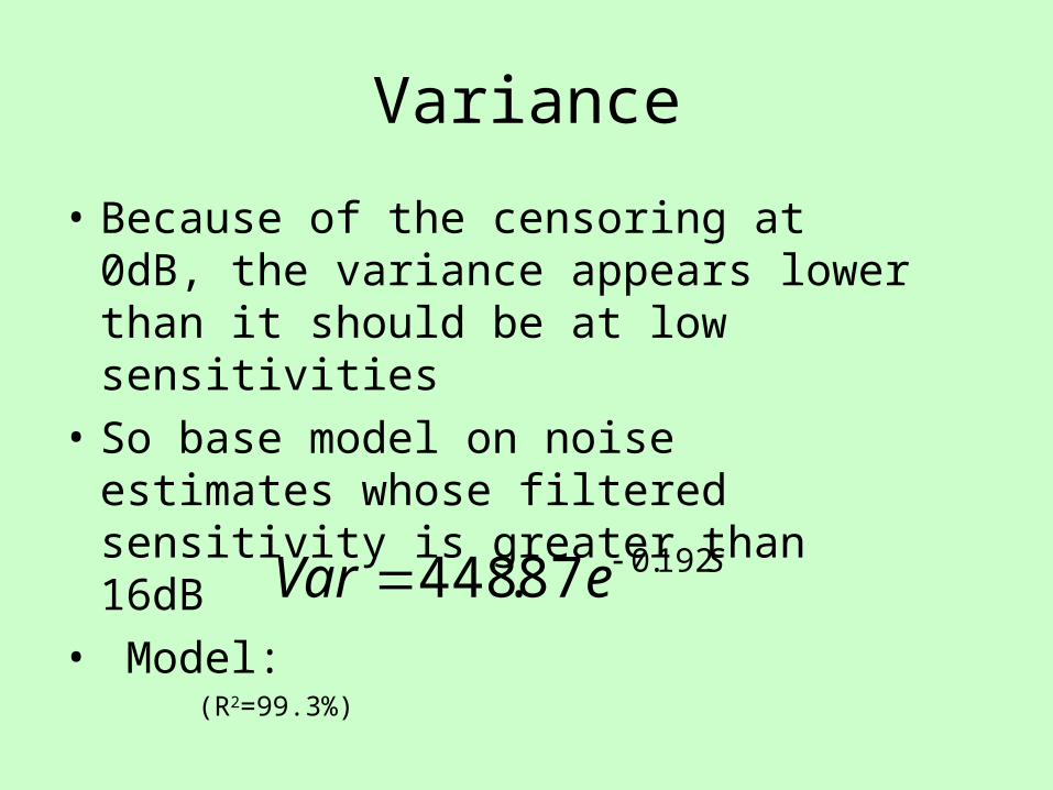
Variance
• Because of the censoring at 0dB, the variance appears lower than it should be at low sensitivities
• So base model on noise estimates whose filtered sensitivity is greater than 16dB
• Model: (R2=99.3%)
SeVar 192.087.448
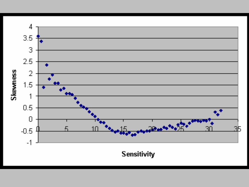

Skewness
• Again, because of the censoring at 0dB, the negative skewness disappears (and becomes positive) at low sensitivities
• So base model on noise estimates whose filtered sensitivity is greater than 16dB
• Model: (R2=87.8%)
5041.10519.0 SSkew
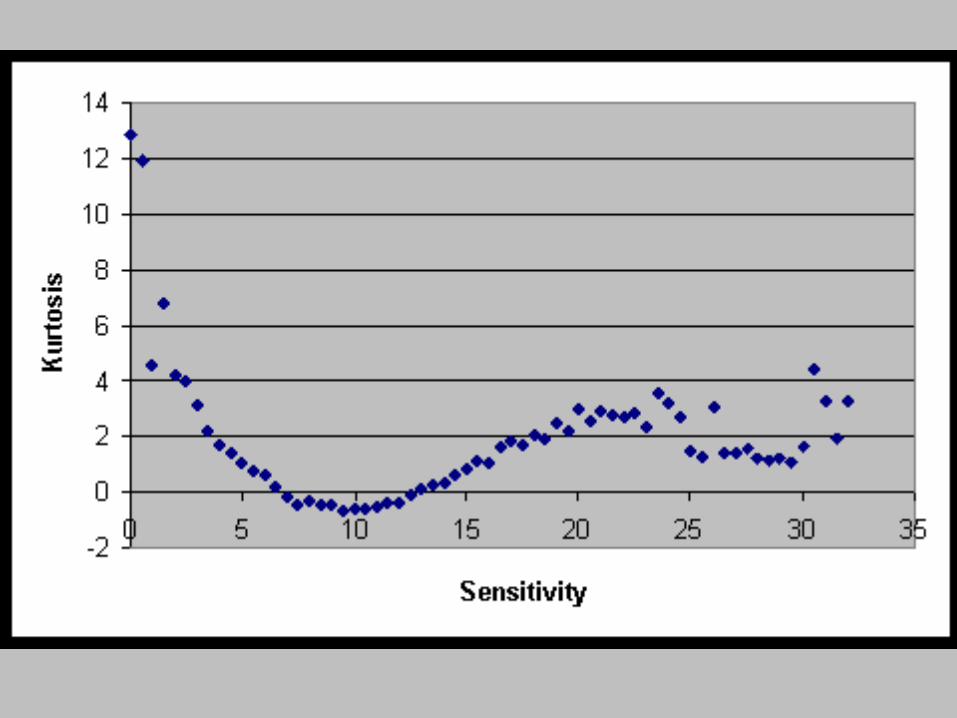

Kurtosis
• Kurtosis is even more affected by the censoring
• There is no discernable pattern for filtered sensitivities greater than 16dB
• So use average value instead:
305.2Kurt

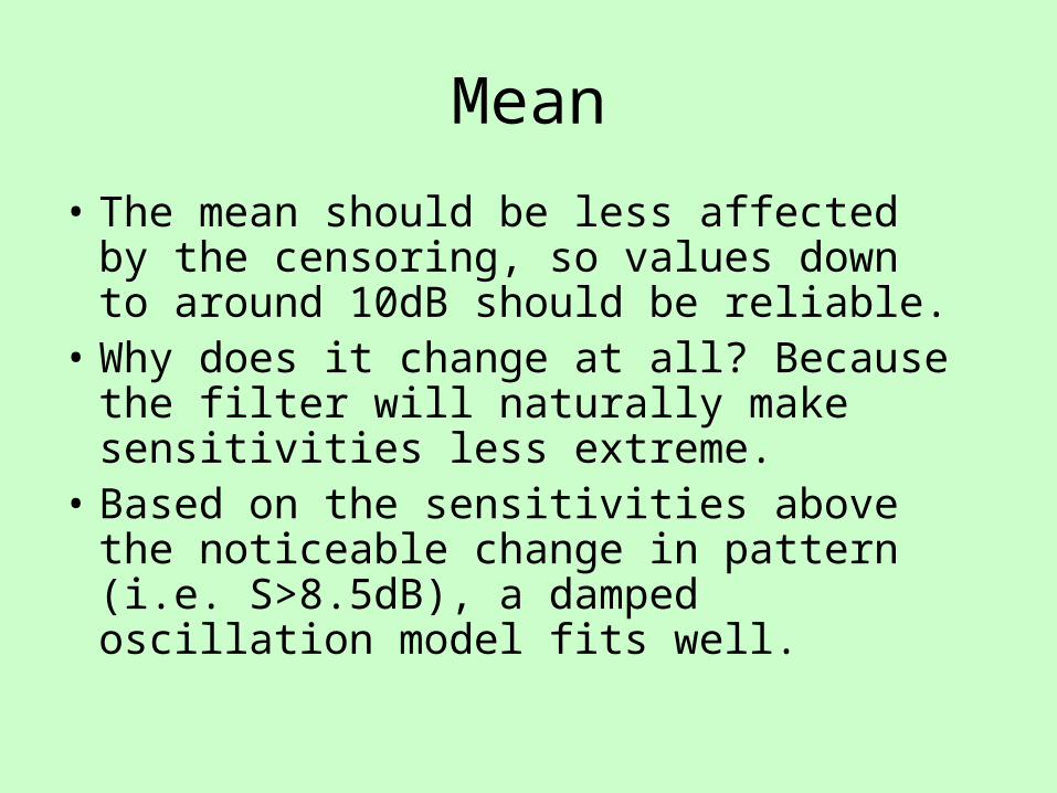
Mean
• The mean should be less affected by the censoring, so values down to around 10dB should be reliable.
• Why does it change at all? Because the filter will naturally make sensitivities less extreme.
• Based on the sensitivities above the noticeable change in pattern (i.e. S>8.5dB), a damped oscillation model fits well.

))4866.1(2034.0sin(5414.6 )4866.1(1154.0 SeMean S
(crosses represent the empirical mean at each sensitivity; dots represent the modelled mean at the same point)

So, we have values for:
MeanVariance
SkewnessKurtosis
of the noise at any given sensitivity.
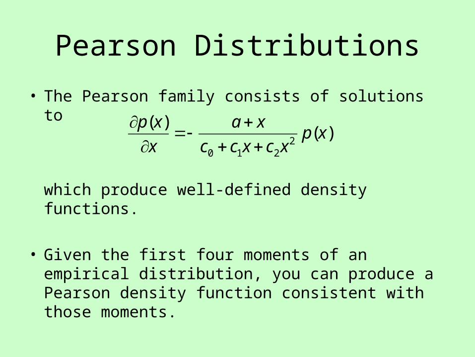
Pearson Distributions
• The Pearson family consists of solutions to
which produce well-defined density functions.
• Given the first four moments of an empirical distribution, you can produce a Pearson density function consistent with those moments.
)()(
2210
xpxcxcc
xa
x
xp
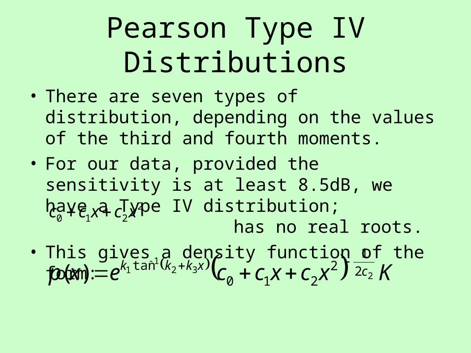
Pearson Type IV Distributions
• There are seven types of distribution, depending on the values of the third and fourth moments.
• For our data, provided the sensitivity is at least 8.5dB, we have a Type IV distribution; has no real roots.
• This gives a density function of the form:
Kxcxccexp cxkkk2
321
1 2
12
210tan)(
2210 xcxcc
Steps to the distribution:
1. Predict the mean, variance, skewness and kurtosis of the distribution
2. Use these to calculate the Pearson constants
3. Use numerical integration to obtain a well-defined density function
4. Adjust the mean of the distribution so that it equals the predicted mean
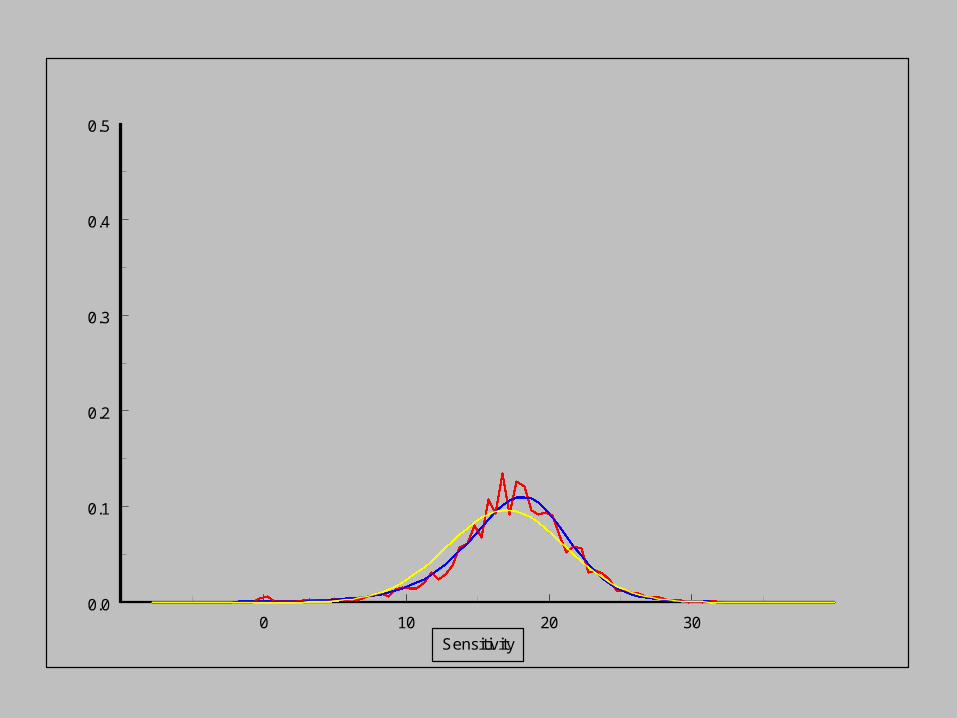
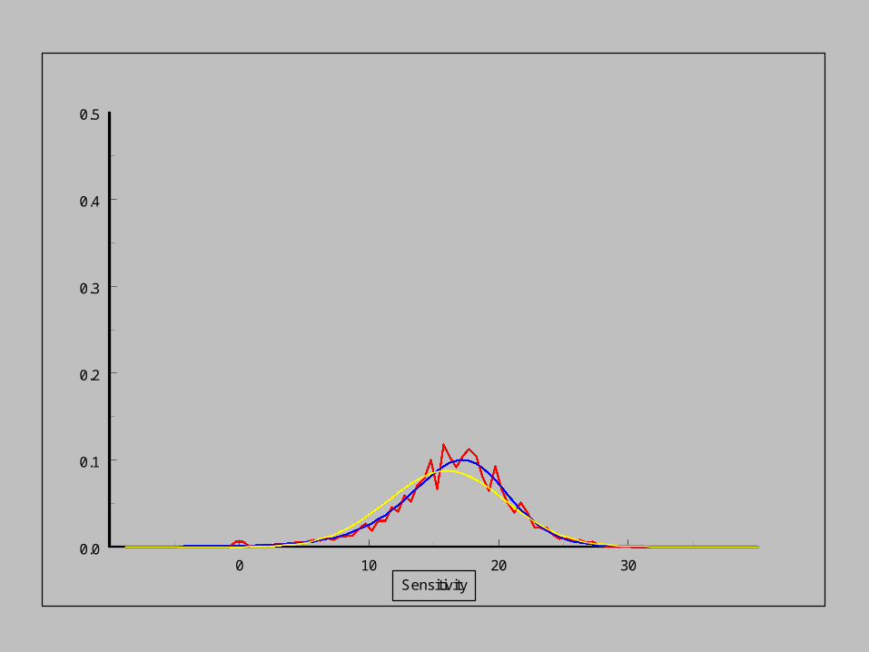
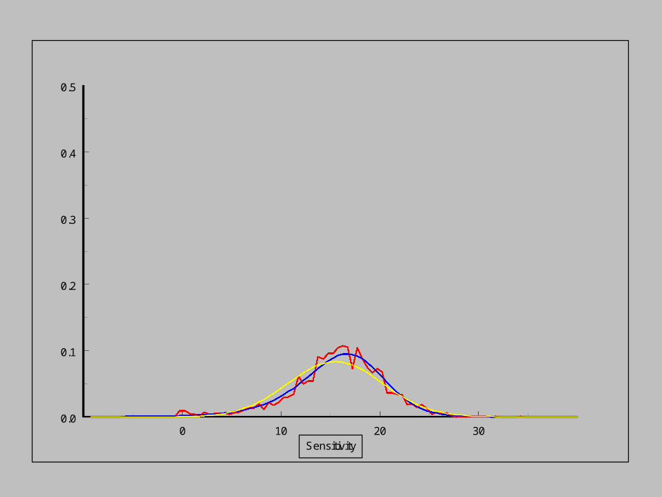
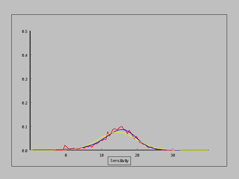
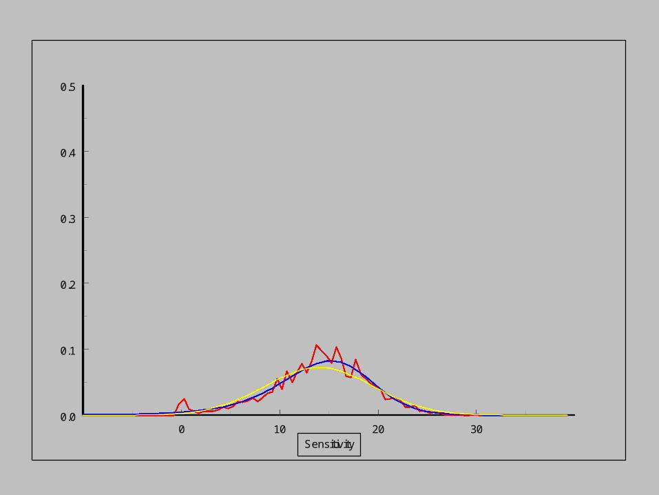
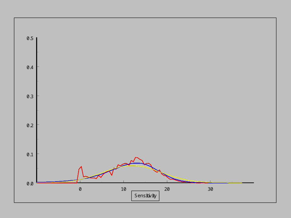
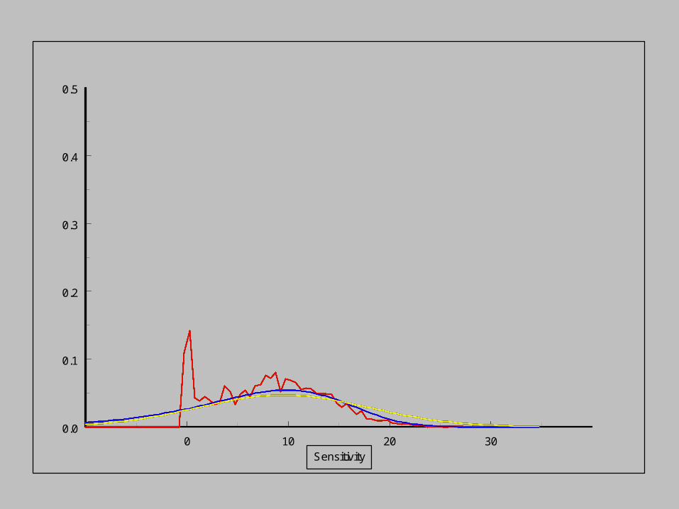
• So, we can model the noise distribution - or equivalently the distribution of the raw sensitivity - at any given input sensitivity.
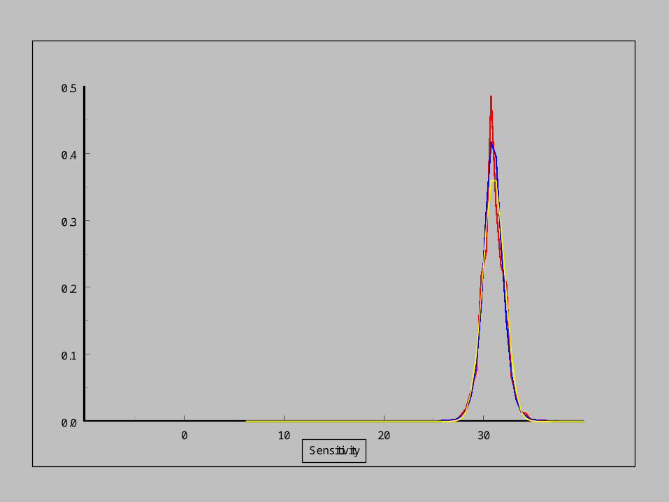
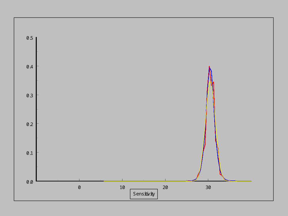
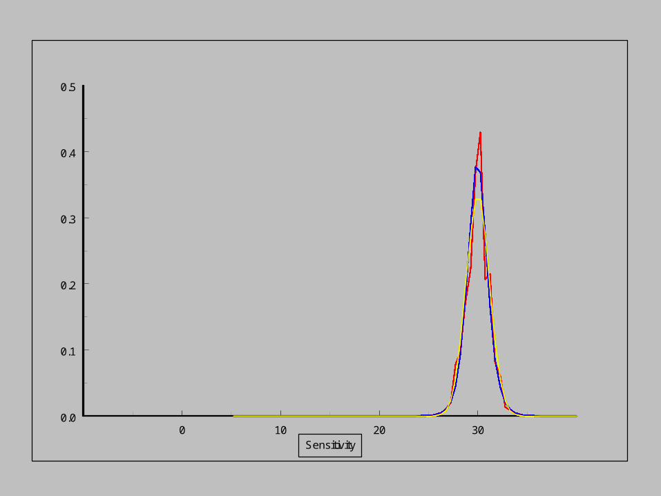
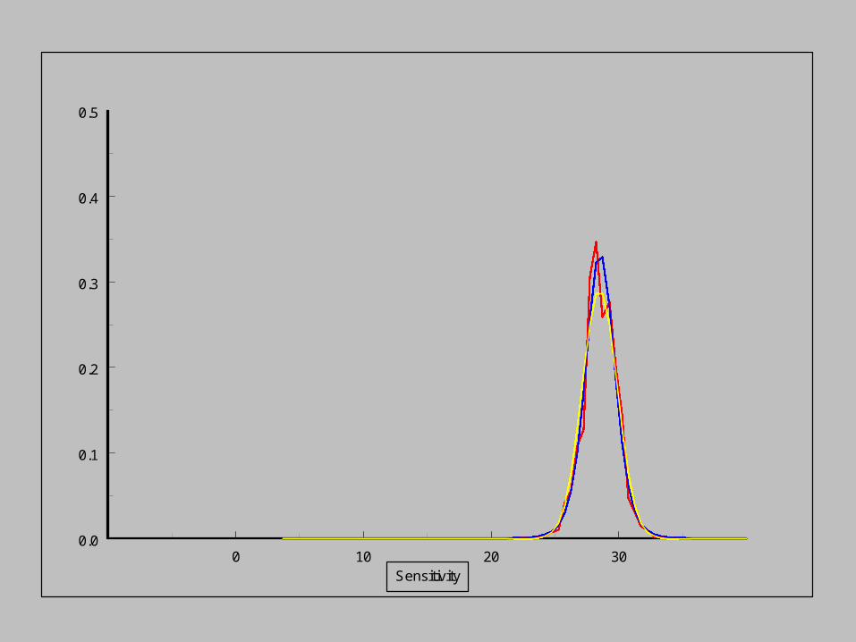
• This model will be compared with the empirical distribution, and with a normal model.

26 28 30 32 34Sensitivity
0.0
0.1
0.2
0.3
0.4
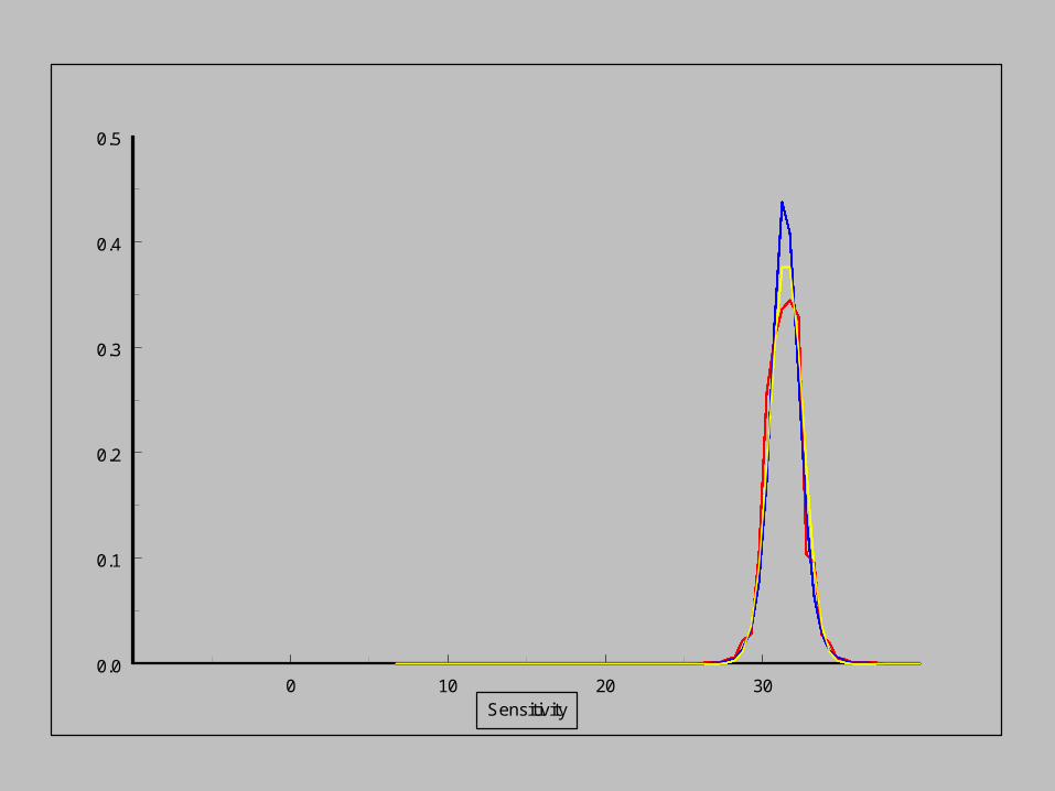
Filtered Sensitivity between 30.25dB and
30.75dB
-10 0 10 20 30Sensitivity
0.00
0.02
0.04
0.06
0.08
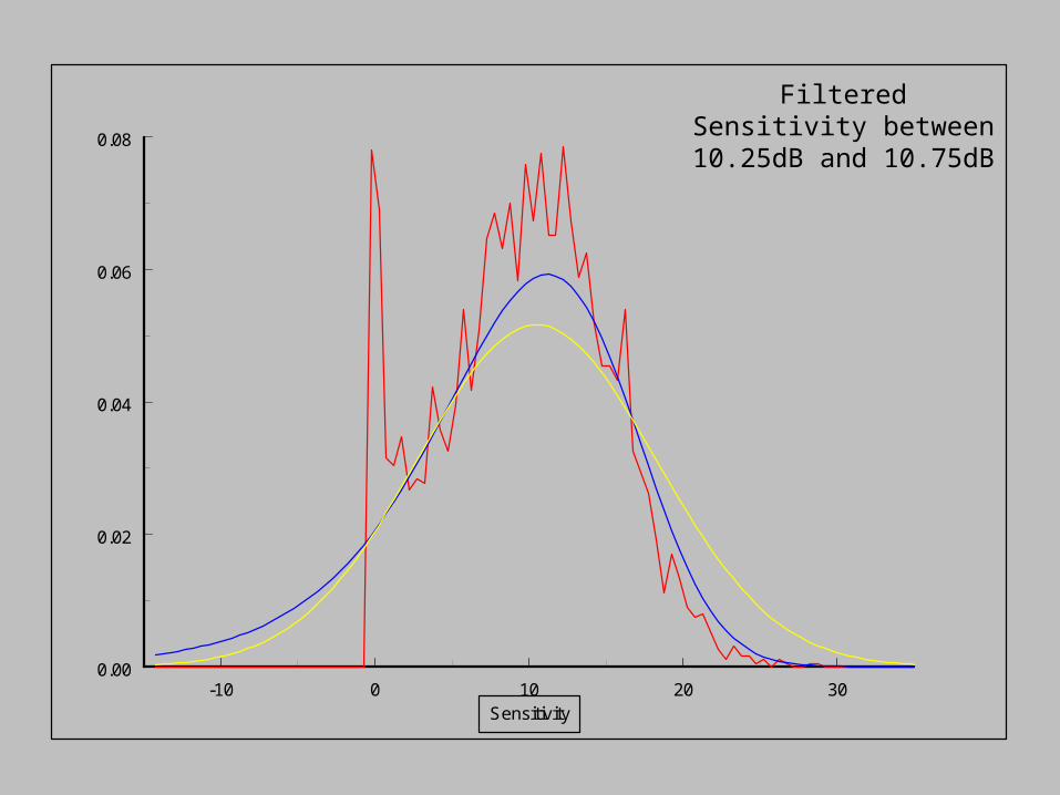
Filtered Sensitivity between 10.25dB and
10.75dB

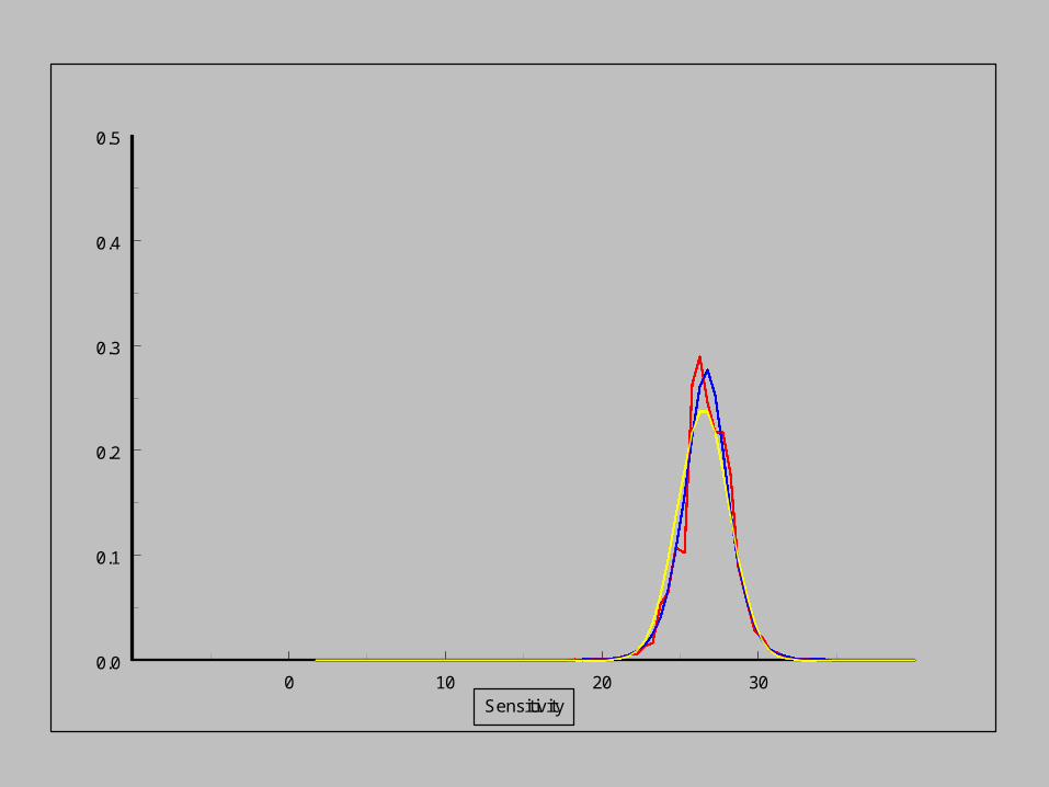
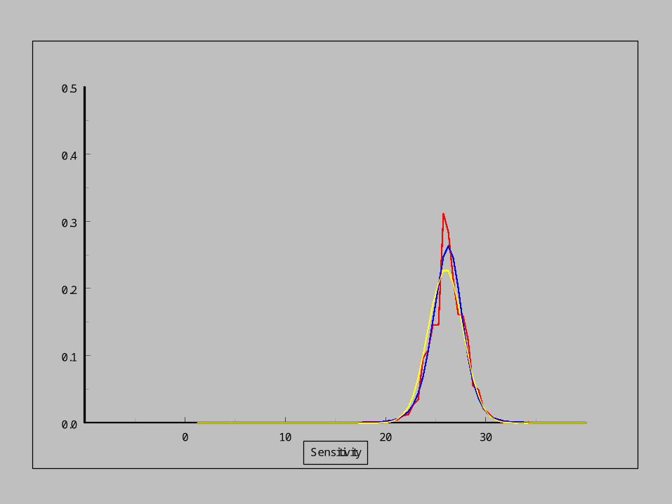
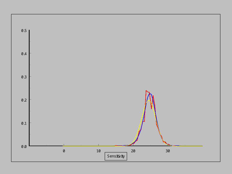
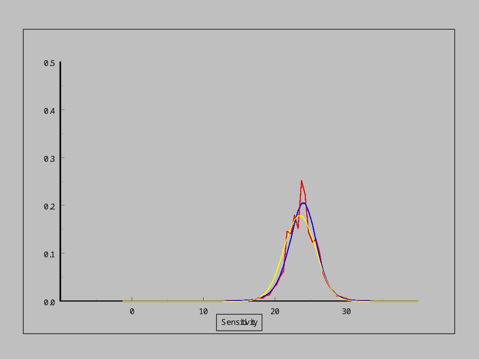
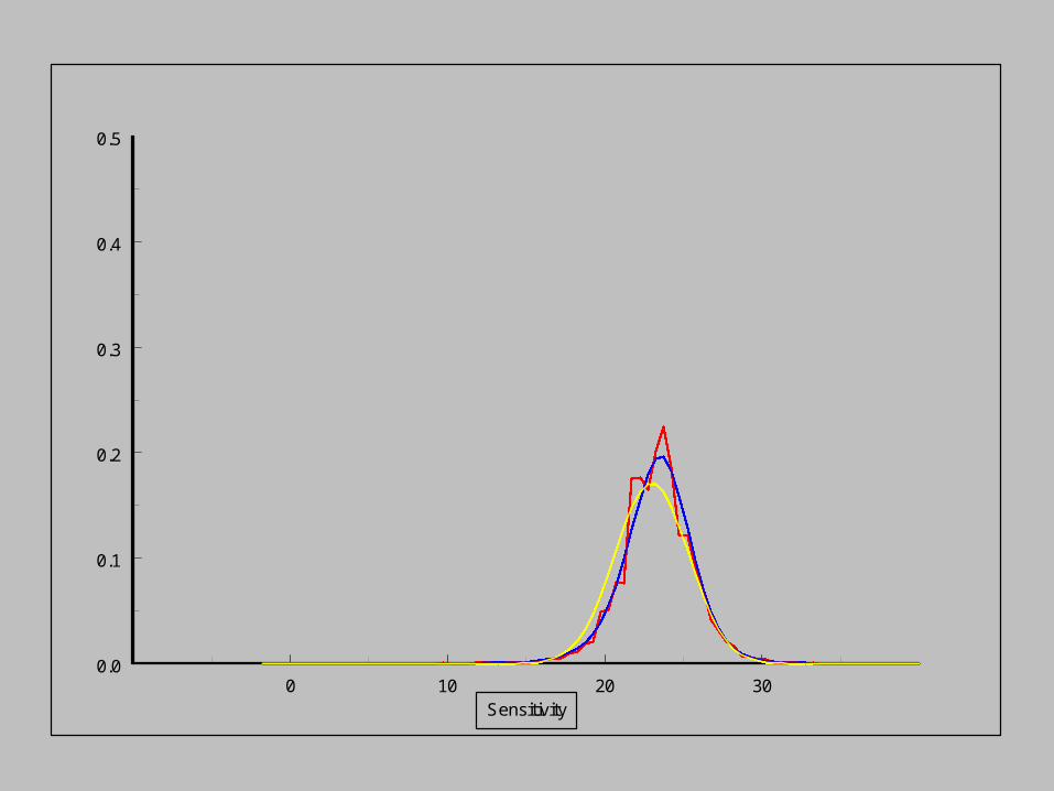
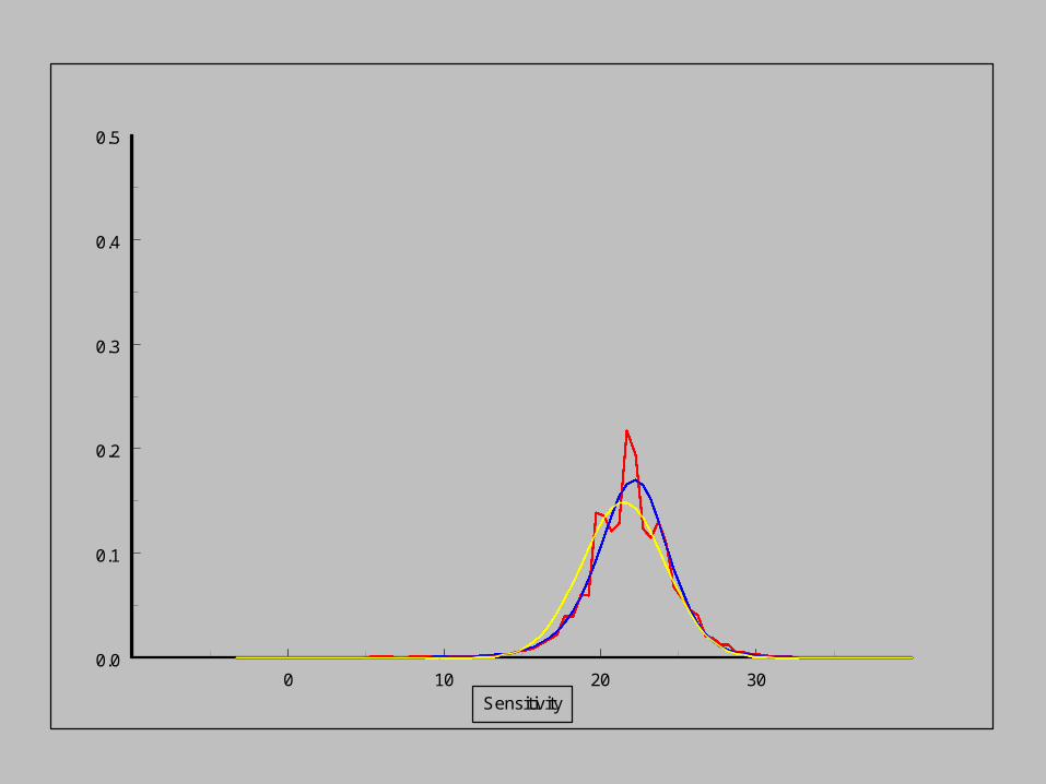
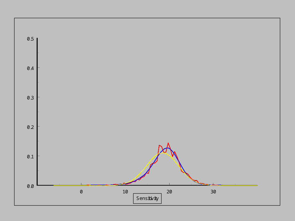
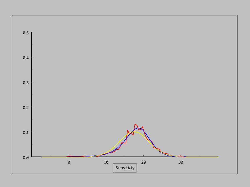
As the sensitivity increases,
the pdf of the noise distribution changes.
Empirical distribution
Modelled distribution
Normal distribution
0 10 20 30Sensitivity
0.0
0.1
0.2
0.3
0.4
0.5
0 10 20 30Sensitivity
0.0
0.1
0.2
0.3
0.4
0.5
0 10 20 30Sensitivity
0.0
0.1
0.2
0.3
0.4
0.5
0 10 20 30Sensitivity
0.0
0.1
0.2
0.3
0.4
0.5

0 10 20 30Sensitivity
0.0
0.1
0.2
0.3
0.4
0.5

0 10 20 30Sensitivity
0.0
0.1
0.2
0.3
0.4
0.5
0 10 20 30Sensitivity
0.0
0.1
0.2
0.3
0.4
0.5

0 10 20 30Sensitivity
0.0
0.1
0.2
0.3
0.4
0.5

0 10 20 30Sensitivity
0.0
0.1
0.2
0.3
0.4
0.5

0 10 20 30Sensitivity
0.0
0.1
0.2
0.3
0.4
0.5
0 10 20 30Sensitivity
0.0
0.1
0.2
0.3
0.4
0.5
0 10 20 30Sensitivity
0.0
0.1
0.2
0.3
0.4
0.5

0 10 20 30Sensitivity
0.0
0.1
0.2
0.3
0.4
0.5

0 10 20 30Sensitivity
0.0
0.1
0.2
0.3
0.4
0.5
0 10 20 30Sensitivity
0.0
0.1
0.2
0.3
0.4
0.5

0 10 20 30Sensitivity
0.0
0.1
0.2
0.3
0.4
0.5
0 10 20 30Sensitivity
0.0
0.1
0.2
0.3
0.4
0.5
0 10 20 30Sensitivity
0.0
0.1
0.2
0.3
0.4
0.5

0 10 20 30Sensitivity
0.0
0.1
0.2
0.3
0.4
0.5

0 10 20 30Sensitivity
0.0
0.1
0.2
0.3
0.4
0.5
0 10 20 30Sensitivity
0.0
0.1
0.2
0.3
0.4
0.5

0 10 20 30Sensitivity
0.0
0.1
0.2
0.3
0.4
0.5

0 10 20 30Sensitivity
0.0
0.1
0.2
0.3
0.4
0.5

0 10 20 30Sensitivity
0.0
0.1
0.2
0.3
0.4
0.5

0 10 20 30Sensitivity
0.0
0.1
0.2
0.3
0.4
0.5

0 10 20 30Sensitivity
0.0
0.1
0.2
0.3
0.4
0.5
0 10 20 30Sensitivity
0.0
0.1
0.2
0.3
0.4
0.5

0 10 20 30Sensitivity
0.0
0.1
0.2
0.3
0.4
0.5
0 10 20 30Sensitivity
0.0
0.1
0.2
0.3
0.4
0.5
0 10 20 30Sensitivity
0.0
0.1
0.2
0.3
0.4
0.5

0 10 20 30Sensitivity
0.0
0.1
0.2
0.3
0.4
0.5
0 10 20 30Sensitivity
0.0
0.1
0.2
0.3
0.4
0.5
0 10 20 30Sensitivity
0.0
0.1
0.2
0.3
0.4
0.5

0 10 20 30Sensitivity
0.0
0.1
0.2
0.3
0.4
0.5
0 10 20 30Sensitivity
0.0
0.1
0.2
0.3
0.4
0.5
0 10 20 30Sensitivity
0.0
0.1
0.2
0.3
0.4
0.5

0 10 20 30Sensitivity
0.0
0.1
0.2
0.3
0.4
0.5

0 10 20 30Sensitivity
0.0
0.1
0.2
0.3
0.4
0.5

0 10 20 30Sensitivity
0.0
0.1
0.2
0.3
0.4
0.5
0 10 20 30Sensitivity
0.0
0.1
0.2
0.3
0.4
0.5

0 10 20 30Sensitivity
0.0
0.1
0.2
0.3
0.4
0.5

0 10 20 30Sensitivity
0.0
0.1
0.2
0.3
0.4
0.5

0 10 20 30Sensitivity
0.0
0.1
0.2
0.3
0.4
0.5

0 10 20 30Sensitivity
0.0
0.1
0.2
0.3
0.4
0.5
0 10 20 30Sensitivity
0.0
0.1
0.2
0.3
0.4
0.5

0 10 20 30Sensitivity
0.0
0.1
0.2
0.3
0.4
0.5

0 10 20 30Sensitivity
0.0
0.1
0.2
0.3
0.4
0.5

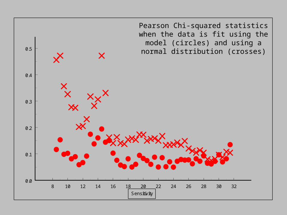
How good is the fit?
• Calculate Pearson chi-squared statistics:
• Compare with the statistics when the noise is modelled by a normal distribution, with mean zero and the same variance
k
i i
ii
e
eo
1
2)(
8 10 12 14 16 18 20 22 24 26 28 30 32
Sensitivity
0.0
0.1
0.2
0.3
0.4
0.5
Pearson Chi-squared statistics when the data is fit using the model (circles) and using a normal distribution (crosses)

• So the fit is much improved.
• The model even performs better when we are extrapolating our predictions for the variance, skewness and kurtosis downwards below 16dB.
Conclusion:
Our new model is better than the current one!

Future Work:
• Test the model against independent data
• Extend the model to one valid below 8dB
• Use the model to simulate visual fields for research in other areas, such as improving testing strategies
The End


Recommended
![Research Article Analysis of Retinal Peripapillary ...downloads.hindawi.com/journals/bmri/2015/636548.pdfretinal degenerations have been described [ , ]. e retinal nerve berlayer(RNFL)iscomposedofretinal-ganglioncell](https://img.pdfslide.us/doc/110x75/612026abd26ded4f3f5438f8/research-article-analysis-of-retinal-peripapillary-retinal-degenerations-have.jpg)