Reliable Approximate Bayesian computation(ABC) model choice via random forests
Christian P. RobertUniversité Paris-Dauphine, Paris & University of Warwick, Coventry
SPA 2015, University of [email protected]
Joint with J.-M. Cornuet, A. Estoup, J.-M. Marin, & P. Pudlo
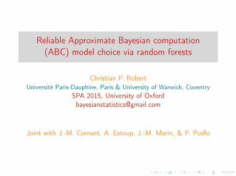
The next MCMSkv meeting:
I Computational Bayes section ofISBA major meeting:
I MCMSki V in Lenzerheide,Switzerland, Jan. 5-7, 2016
I MCMC, pMCMC, SMC2, HMC,ABC, (ultra-) high-dimensionalcomputation, BNP, QMC, deeplearning, &tc
I Plenary speakers: S. Scott, S.Fienberg, D. Dunson, K.Latuszynski, T. Lelièvre
I Call for contributed 9 sessionsand tutorials opened
I “Switzerland in January, whereelse...?!"
Outline
Intractable likelihoods
ABC methods
ABC for model choice
ABC model choice via random forests
intractable likelihood
Case of a well-defined statistical model where the likelihoodfunction
`(θ|y) = f (y1, . . . , yn|θ)
I is (really!) not available in closed formI cannot (easily!) be either completed or demarginalisedI cannot be (at all!) estimated by an unbiased estimatorI examples of latent variable models of high dimension, including
combinatorial structures (trees, graphs), missing constantf (x |θ) = g(y , θ)
/Z (θ) (eg. Markov random fields, exponential
graphs,. . . )c© Prohibits direct implementation of a generic MCMC algorithmlike Metropolis–Hastings which gets stuck exploring missingstructures
intractable likelihood
Case of a well-defined statistical model where the likelihoodfunction
`(θ|y) = f (y1, . . . , yn|θ)
I is (really!) not available in closed formI cannot (easily!) be either completed or demarginalisedI cannot be (at all!) estimated by an unbiased estimator
c© Prohibits direct implementation of a generic MCMC algorithmlike Metropolis–Hastings which gets stuck exploring missingstructures
Necessity is the mother of invention
Case of a well-defined statistical model where the likelihoodfunction
`(θ|y) = f (y1, . . . , yn|θ)
is out of reach
Empirical A to the original B problemI Degrading the data precision down to tolerance level εI Replacing the likelihood with a non-parametric approximation
based on simulationsI Summarising/replacing the data with insufficient statistics
Approximate Bayesian computation
Intractable likelihoods
ABC methodsGenesis of ABCabc of ABCSummary statistic
ABC for model choice
ABC model choice via randomforests
Genetic background of ABC
skip genetics
ABC is a recent computational technique that only requires beingable to sample from the likelihood f (·|θ)
This technique stemmed from population genetics models, about15 years ago, and population geneticists still significantly contributeto methodological developments of ABC.
[Griffith & al., 1997; Tavaré & al., 1999]
Demo-genetic inference
Each model is characterized by a set of parameters θ that coverhistorical (time divergence, admixture time ...), demographics(population sizes, admixture rates, migration rates, ...) and genetic(mutation rate, ...) factors
The goal is to estimate these parameters from a dataset ofpolymorphism (DNA sample) y observed at the present time
Problem:most of the time, we cannot calculate the likelihood of thepolymorphism data f (y|θ)...
Kingman’s colaescent
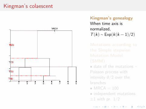
Kingman’s genealogyWhen time axis isnormalized,T (k) ∼ Exp(k(k − 1)/2)
Mutations according tothe Simple stepwiseMutation Model(SMM)• date of the mutations ∼Poisson process withintensity θ/2 over thebranches• MRCA = 100• independent mutations:±1 with pr. 1/2
Kingman’s colaescent
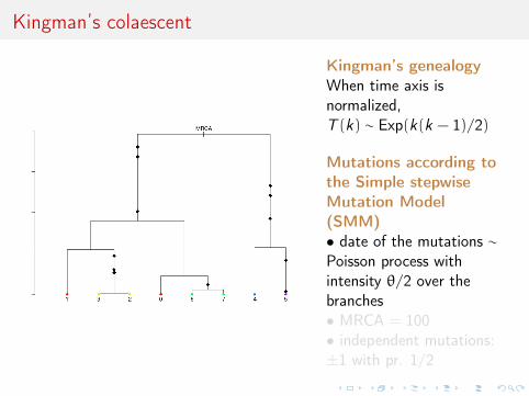
Kingman’s genealogyWhen time axis isnormalized,T (k) ∼ Exp(k(k − 1)/2)
Mutations according tothe Simple stepwiseMutation Model(SMM)• date of the mutations ∼Poisson process withintensity θ/2 over thebranches• MRCA = 100• independent mutations:±1 with pr. 1/2
Kingman’s colaescent
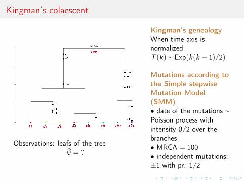
Observations: leafs of the treeθ̂ = ?
Kingman’s genealogyWhen time axis isnormalized,T (k) ∼ Exp(k(k − 1)/2)
Mutations according tothe Simple stepwiseMutation Model(SMM)• date of the mutations ∼Poisson process withintensity θ/2 over thebranches• MRCA = 100• independent mutations:±1 with pr. 1/2
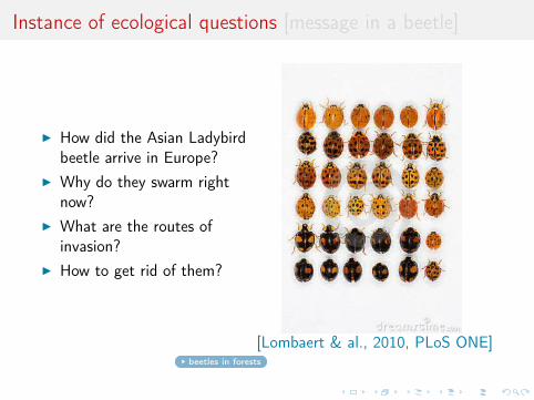
Instance of ecological questions [message in a beetle]
I How did the Asian Ladybirdbeetle arrive in Europe?
I Why do they swarm rightnow?
I What are the routes ofinvasion?
I How to get rid of them?
[Lombaert & al., 2010, PLoS ONE]beetles in forests
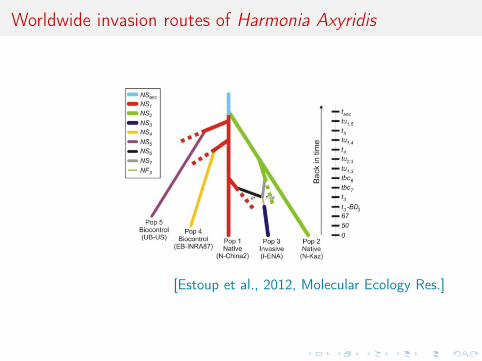
Worldwide invasion routes of Harmonia Axyridis
[Estoup et al., 2012, Molecular Ecology Res.]
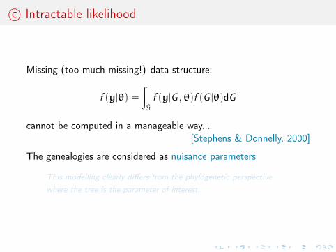
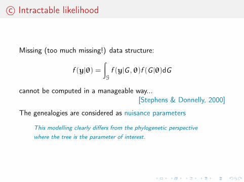
c© Intractable likelihood
Missing (too much missing!) data structure:
f (y|θ) =∫G
f (y|G ,θ)f (G |θ)dG
cannot be computed in a manageable way...[Stephens & Donnelly, 2000]
The genealogies are considered as nuisance parameters
This modelling clearly differs from the phylogenetic perspectivewhere the tree is the parameter of interest.
A?B?C?
I A stands for approximate[wrong likelihood /picture]
I B stands for BayesianI C stands for computation
[producing a parametersample]
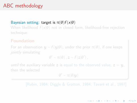
ABC methodology
Bayesian setting: target is π(θ)f (x |θ)When likelihood f (x |θ) not in closed form, likelihood-free rejectiontechnique:
FoundationFor an observation y ∼ f (y|θ), under the prior π(θ), if one keepsjointly simulating
θ′ ∼ π(θ) , z ∼ f (z|θ′) ,
until the auxiliary variable z is equal to the observed value, z = y,then the selected
θ′ ∼ π(θ|y)
[Rubin, 1984; Diggle & Gratton, 1984; Tavaré et al., 1997]
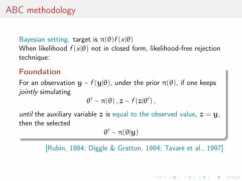
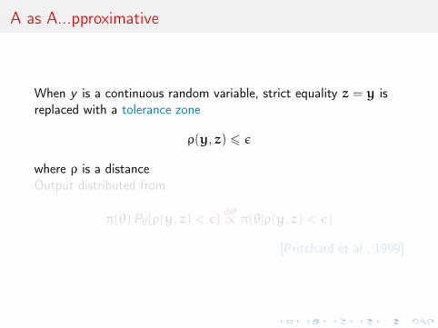
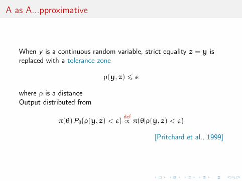
A as A...pproximative
When y is a continuous random variable, strict equality z = y isreplaced with a tolerance zone
ρ(y, z) 6 ε
where ρ is a distanceOutput distributed from
π(θ)Pθ{ρ(y, z) < ε} def∝ π(θ|ρ(y, z) < ε)
[Pritchard et al., 1999]
A as A...pproximative
When y is a continuous random variable, strict equality z = y isreplaced with a tolerance zone
ρ(y, z) 6 ε
where ρ is a distanceOutput distributed from
π(θ)Pθ{ρ(y, z) < ε}def∝ π(θ|ρ(y, z) < ε)
[Pritchard et al., 1999]
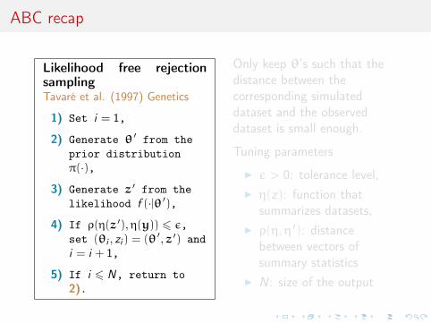
ABC recap
Likelihood free rejectionsamplingTavaré et al. (1997) Genetics
1) Set i = 1,
2) Generate θ ′ from theprior distributionπ(·),
3) Generate z ′ from thelikelihood f (·|θ ′),
4) If ρ(η(z ′),η(y)) 6 ε,set (θi , zi ) = (θ ′, z ′) andi = i + 1,
5) If i 6 N, return to2).
Only keep θ’s such that thedistance between thecorresponding simulateddataset and the observeddataset is small enough.
Tuning parameters
I ε > 0: tolerance level,I η(z): function that
summarizes datasets,I ρ(η,η ′): distance
between vectors ofsummary statistics
I N: size of the output
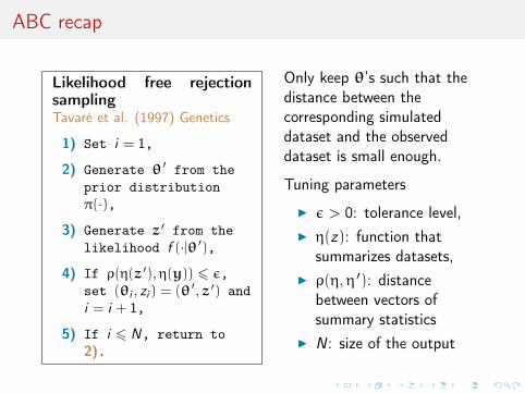
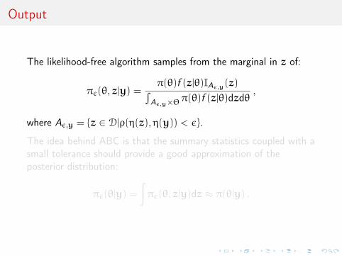
Output
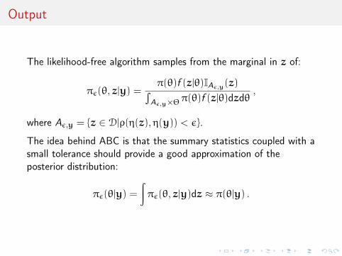
The likelihood-free algorithm samples from the marginal in z of:
πε(θ, z|y) =π(θ)f (z|θ)IAε,y(z)∫
Aε,y×Θ π(θ)f (z|θ)dzdθ,
where Aε,y = {z ∈ D|ρ(η(z),η(y)) < ε}.
The idea behind ABC is that the summary statistics coupled with asmall tolerance should provide a good approximation of theposterior distribution:
πε(θ|y) =
∫πε(θ, z|y)dz ≈ π(θ|y) .
Output
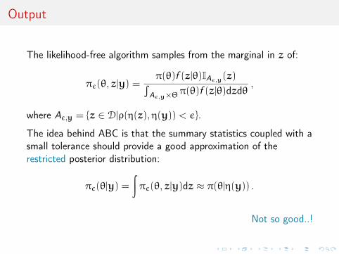
The likelihood-free algorithm samples from the marginal in z of:
πε(θ, z|y) =π(θ)f (z|θ)IAε,y(z)∫
Aε,y×Θ π(θ)f (z|θ)dzdθ,
where Aε,y = {z ∈ D|ρ(η(z),η(y)) < ε}.
The idea behind ABC is that the summary statistics coupled with asmall tolerance should provide a good approximation of therestricted posterior distribution:
πε(θ|y) =
∫πε(θ, z|y)dz ≈ π(θ|η(y)) .
Not so good..!
Comments
I Role of distance paramount(because ε 6= 0)
I Scaling of components ofη(y) is also determinant
I ε matters little if “smallenough"
I representative of “curse ofdimensionality"
I small is beautiful!I the data as a whole may be
paradoxically weaklyinformative for ABC
Which summary?
Fundamental difficulty of the choice of the summary statistic whenthere is no non-trivial sufficient statistics [except when done by theexperimenters in the field]
I Loss of statistical information balanced against gain in dataroughening
I Approximation error and information loss remain unknownI Choice of statistics induces choice of distance function towards
standardisation
I may be imposed for external/practical reasons (e.g., DIYABC)I may gather several non-B point estimates [the more the
merrier]I can [machine-]learn about efficient combination
attempts at summaries
How to choose the set of summary statistics?
I Joyce and Marjoram (2008, SAGMB)I Fearnhead and Prangle (2012, JRSS B)I Ratmann et al. (2012, PLOS Comput. Biol)I Blum et al. (2013, Statistical Science)I LDA selection of Estoup & al. (2012, Mol. Ecol. Res.)
ABC for model choice
Intractable likelihoods
ABC methods
ABC for model choice
ABC model choice via random forests

ABC model choice
ABC model choiceA) Generate large set of
(m,θ, z) from theBayesian predictive,π(m)πm(θ)fm(z|θ)
B) Keep particles (m,θ, z)such thatρ(η(y),η(z)) 6 ε
C) For each m, returnp̂m = proportion of mamong remainingparticles
If ε tuned towards k resultingparticles, then p̂m k-nearestneighbor estimate of
P({M = m
}∣∣∣η(y))Approximating posteriorprob’s of models = regressionproblem where
I response is 1{M = m
},
I covariates are summarystatistics η(z),
I loss is, e.g., L2
Method of choice in DIYABCis local polytomous logisticregression
Machine learning perspective [paradigm shift]
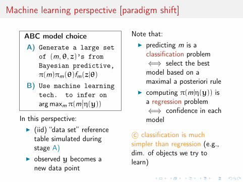
ABC model choiceA) Generate a large set
of (m,θ, z)’s fromBayesian predictive,π(m)πm(θ)fm(z|θ)
B) Use machine learningtech. to infer onargmaxm π(m
∣∣η(y))In this perspective:
I (iid) “data set” referencetable simulated duringstage A)
I observed y becomes anew data point
Note that:I predicting m is a
classification problem⇐⇒ select the bestmodel based on amaximal a posteriori rule
I computing π(m|η(y)) isa regression problem⇐⇒ confidence in eachmodel
c© classification is muchsimpler than regression (e.g.,dim. of objects we try tolearn)
Warning
the lost of information induced by using non sufficientsummary statistics is a genuine problem
Fundamental discrepancy between the genuine Bayesfactors/posterior probabilities and the Bayes factors based onsummary statistics. See, e.g.,
I Didelot et al. (2011, Bayesian analysis)I X et al. (2011, PNAS)I Marin et al. (2014, JRSS B)I . . .
Call instead for machine learning approach able to handle with alarge number of correlated summary statistics:
random forests well suited for that task
ABC model choice via random forests
Intractable likelihoods
ABC methods
ABC for model choice
ABC model choice via random forestsRandom forestsABC with random forestsIllustrations
Leaning towards machine learning
Main notions:I ABC-MC seen as learning about which model is most
appropriate from a huge (reference) tableI exploiting a large number of summary statistics not an issue
for machine learning methods intended to estimate efficientcombinations
I abandoning (temporarily?) the idea of estimating posteriorprobabilities of the models, poorly approximated by machinelearning methods, and replacing those by posterior predictiveexpected loss
I estimating posterior probabilities of the selected model bymachine learning methods
Random forests
Technique that stemmed from Leo Breiman’s bagging (or bootstrapaggregating) machine learning algorithm for both classification andregression
[Breiman, 1996]
Improved classification performances by averaging overclassification schemes of randomly generated training sets, creatinga “forest" of (CART) decision trees, inspired by Amit and Geman(1997) ensemble learning
[Breiman, 2001]
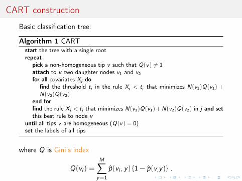
CART construction
Basic classification tree:
Algorithm 1 CARTstart the tree with a single rootrepeat
pick a non-homogeneous tip v such that Q(v) 6= 1attach to v two daughter nodes v1 and v2
for all covariates Xj dofind the threshold tj in the rule Xj < tj that minimizes N(v1)Q(v1) +N(v2)Q(v2)
end forfind the rule Xj < tj that minimizes N(v1)Q(v1)+N(v2)Q(v2) in j and setthis best rule to node v
until all tips v are homogeneous (Q(v) = 0)set the labels of all tips
where Q is Gini’s index
Q(vi ) =
M∑y=1
p̂(vi , y) {1− p̂(v,y)} .
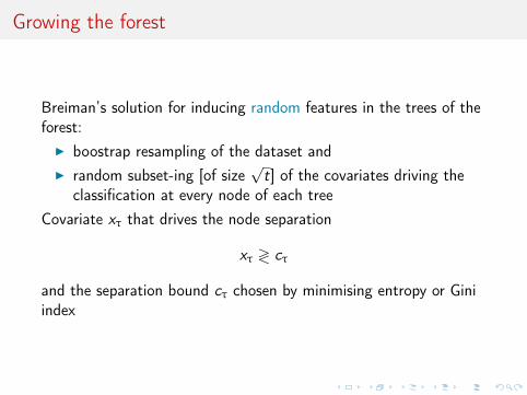
Growing the forest
Breiman’s solution for inducing random features in the trees of theforest:
I boostrap resampling of the dataset andI random subset-ing [of size
√t] of the covariates driving the
classification at every node of each treeCovariate xτ that drives the node separation
xτ ≷ cτ
and the separation bound cτ chosen by minimising entropy or Giniindex
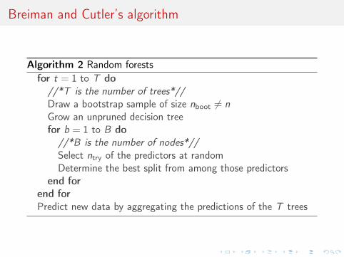
Breiman and Cutler’s algorithm
Algorithm 2 Random forestsfor t = 1 to T do
//*T is the number of trees*//Draw a bootstrap sample of size nboot 6= nGrow an unpruned decision treefor b = 1 to B do
//*B is the number of nodes*//Select ntry of the predictors at randomDetermine the best split from among those predictors
end forend forPredict new data by aggregating the predictions of the T trees
ABC with random forests
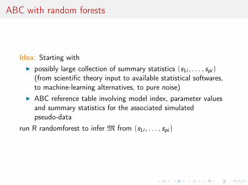
Idea: Starting withI possibly large collection of summary statistics (s1i , . . . , spi )
(from scientific theory input to available statistical softwares,to machine-learning alternatives, to pure noise)
I ABC reference table involving model index, parameter valuesand summary statistics for the associated simulatedpseudo-data
run R randomforest to infer M from (s1i , . . . , spi )
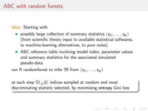
ABC with random forests
Idea: Starting withI possibly large collection of summary statistics (s1i , . . . , spi )
(from scientific theory input to available statistical softwares,to machine-learning alternatives, to pure noise)
I ABC reference table involving model index, parameter valuesand summary statistics for the associated simulatedpseudo-data
run R randomforest to infer M from (s1i , . . . , spi )
at each step O(√
p) indices sampled at random and mostdiscriminating statistic selected, by minimising entropy Gini loss
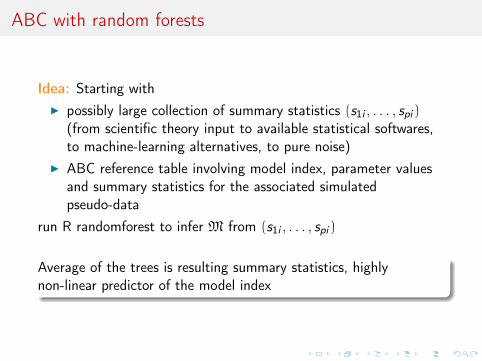
ABC with random forests
Idea: Starting withI possibly large collection of summary statistics (s1i , . . . , spi )
(from scientific theory input to available statistical softwares,to machine-learning alternatives, to pure noise)
I ABC reference table involving model index, parameter valuesand summary statistics for the associated simulatedpseudo-data
run R randomforest to infer M from (s1i , . . . , spi )
Average of the trees is resulting summary statistics, highlynon-linear predictor of the model index
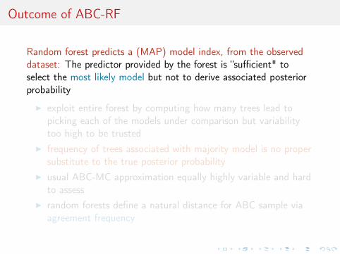
Outcome of ABC-RF
Random forest predicts a (MAP) model index, from the observeddataset: The predictor provided by the forest is “sufficient" toselect the most likely model but not to derive associated posteriorprobability
I exploit entire forest by computing how many trees lead topicking each of the models under comparison but variabilitytoo high to be trusted
I frequency of trees associated with majority model is no propersubstitute to the true posterior probability
I usual ABC-MC approximation equally highly variable and hardto assess
I random forests define a natural distance for ABC sample viaagreement frequency
...antiquated...
Posterior predictive expected losses
We suggest replacing unstable approximation of
P(M = m|xo)
with xo observed sample and m model index, by average of theselection errors across all models given the data xo ,
P(M̂(X ) 6= M|xo)
where pair (M, X ) generated from the predictive∫f (x |θ)π(θ,M|xo)dθ
and M̂(x) denotes the random forest model (MAP) predictor
...antiquated...
Posterior predictive expected losses
Arguments:I Bayesian estimate of the posterior errorI integrates error over most likely part of the parameter spaceI gives an averaged error rather than the posterior probability of
the null hypothesisI easily computed: Given ABC subsample of parameters from
reference table, simulate pseudo-samples associated with thoseand derive error frequency
new!!!
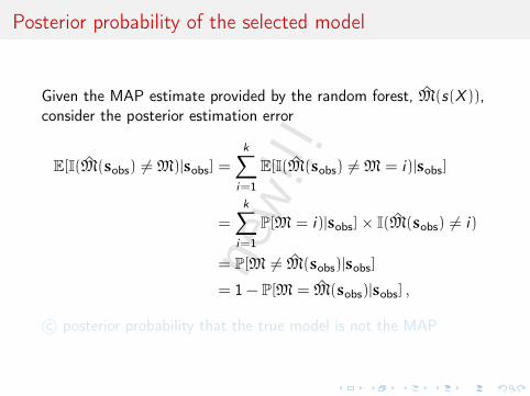
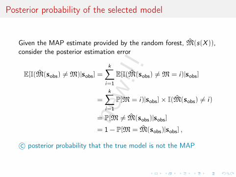
Posterior probability of the selected model
Given the MAP estimate provided by the random forest, M̂(s(X )),consider the posterior estimation error
E[I(M̂(sobs) 6= M)|sobs] =
k∑i=1
E[I(M̂(sobs) 6= M = i)|sobs]
=
k∑i=1
P[M = i)|sobs]× I(M̂(sobs) 6= i)
= P[M 6= M̂(sobs)|sobs]
= 1− P[M = M̂(sobs)|sobs] ,
c© posterior probability that the true model is not the MAP
new!!!
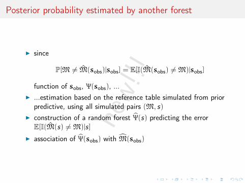
Posterior probability estimated by another forest
I since
P[M 6= M̂(sobs)|sobs] = E[I(M̂(sobs) 6= M)|sobs]
function of sobs, Ψ(sobs), ...I ...estimation based on the reference table simulated from prior
predictive, using all simulated pairs (M, s)I construction of a random forest Ψ̂(s) predicting the error
E[I(M̂(s) 6= M)|s]I association of Ψ̂(sobs) with M̂(sobs)
new!!!
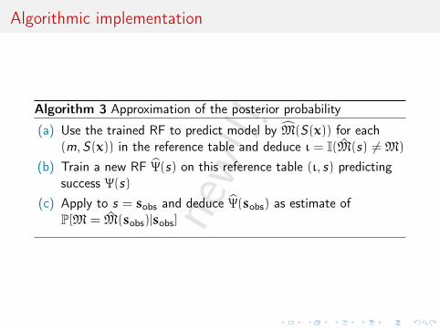
Algorithmic implementation
Algorithm 3 Approximation of the posterior probability
(a) Use the trained RF to predict model by M̂(S(x)) for each(m, S(x)) in the reference table and deduce ι = I(M̂(s) 6= M)
(b) Train a new RF Ψ̂(s) on this reference table (ι, s) predictingsuccess Ψ(s)
(c) Apply to s = sobs and deduce Ψ̂(sobs) as estimate ofP[M = M̂(sobs)|sobs]
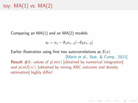
toy: MA(1) vs. MA(2)
Comparing an MA(1) and an MA(2) models:
xt = εt − ϑ1εt−1[−ϑ2εt−2]
Earlier illustration using first two autocorrelations as S(x)[Marin et al., Stat. & Comp., 2011]
Result #1: values of p(m|x) [obtained by numerical integration]and p(m|S(x)) [obtained by mixing ABC outcome and densityestimation] highly differ!
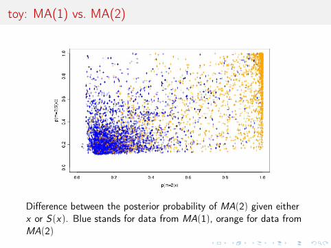
toy: MA(1) vs. MA(2)
Difference between the posterior probability of MA(2) given eitherx or S(x). Blue stands for data from MA(1), orange for data fromMA(2)
toy: MA(1) vs. MA(2)
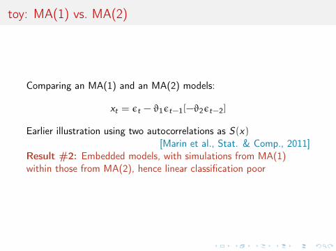
Comparing an MA(1) and an MA(2) models:
xt = εt − ϑ1εt−1[−ϑ2εt−2]
Earlier illustration using two autocorrelations as S(x)[Marin et al., Stat. & Comp., 2011]
Result #2: Embedded models, with simulations from MA(1)within those from MA(2), hence linear classification poor
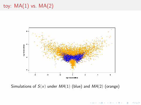
toy: MA(1) vs. MA(2)
Simulations of S(x) under MA(1) (blue) and MA(2) (orange)
toy: MA(1) vs. MA(2)
Comparing an MA(1) and an MA(2) models:
xt = εt − ϑ1εt−1[−ϑ2εt−2]
Earlier illustration using two autocorrelations as S(x)[Marin et al., Stat. & Comp., 2011]
Result #3: On such a small dimension problem, random forestsshould come second to k-nn ou kernel discriminant analyses
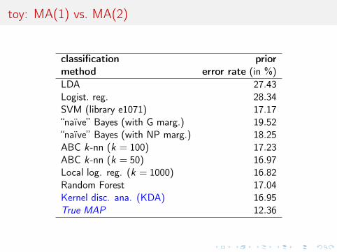
toy: MA(1) vs. MA(2)
classification priormethod error rate (in %)LDA 27.43Logist. reg. 28.34SVM (library e1071) 17.17“naïve” Bayes (with G marg.) 19.52“naïve” Bayes (with NP marg.) 18.25ABC k-nn (k = 100) 17.23ABC k-nn (k = 50) 16.97Local log. reg. (k = 1000) 16.82Random Forest 17.04Kernel disc. ana. (KDA) 16.95True MAP 12.36
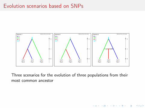
Evolution scenarios based on SNPs
Three scenarios for the evolution of three populations from theirmost common ancestor
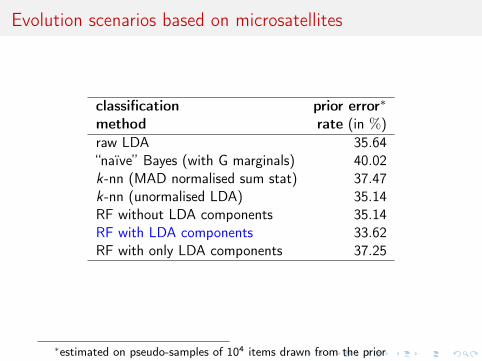
Evolution scenarios based on microsatellites
classification prior error∗
method rate (in %)raw LDA 35.64“naïve” Bayes (with G marginals) 40.02k-nn (MAD normalised sum stat) 37.47k-nn (unormalised LDA) 35.14RF without LDA components 35.14RF with LDA components 33.62RF with only LDA components 37.25
∗estimated on pseudo-samples of 104 items drawn from the prior
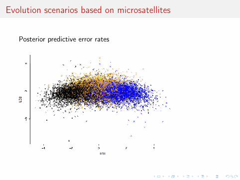
Evolution scenarios based on microsatellites
Posterior predictive error rates
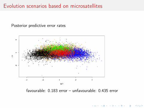
Evolution scenarios based on microsatellites
Posterior predictive error rates
favourable: 0.183 error – unfavourable: 0.435 error
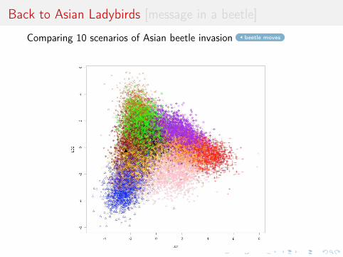
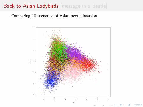
Back to Asian Ladybirds [message in a beetle]
Comparing 10 scenarios of Asian beetle invasion beetle moves
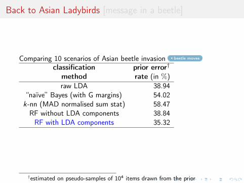
Back to Asian Ladybirds [message in a beetle]
Comparing 10 scenarios of Asian beetle invasion beetle moves
classification prior error†
method rate (in %)raw LDA 38.94
“naïve” Bayes (with G margins) 54.02k-nn (MAD normalised sum stat) 58.47RF without LDA components 38.84RF with LDA components 35.32
†estimated on pseudo-samples of 104 items drawn from the prior
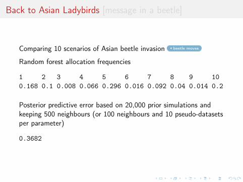
Back to Asian Ladybirds [message in a beetle]
Comparing 10 scenarios of Asian beetle invasion beetle moves
Random forest allocation frequencies
1 2 3 4 5 6 7 8 9 100.168 0.1 0.008 0.066 0.296 0.016 0.092 0.04 0.014 0.2
Posterior predictive error based on 20,000 prior simulations andkeeping 500 neighbours (or 100 neighbours and 10 pseudo-datasetsper parameter)
0.3682
Back to Asian Ladybirds [message in a beetle]
Comparing 10 scenarios of Asian beetle invasion
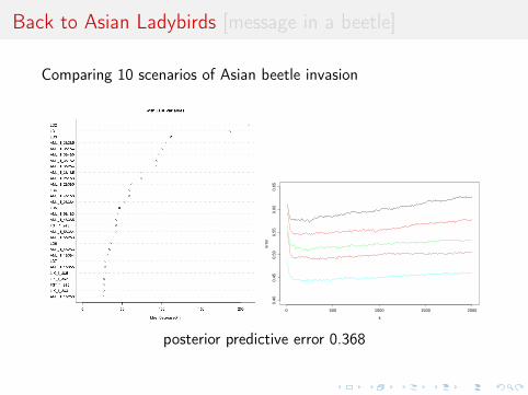
Back to Asian Ladybirds [message in a beetle]
Comparing 10 scenarios of Asian beetle invasion
0 500 1000 1500 2000
0.40
0.45
0.50
0.55
0.60
0.65
k
erro
r
posterior predictive error 0.368
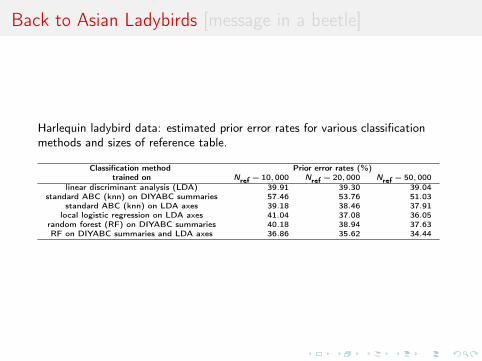
Back to Asian Ladybirds [message in a beetle]
Harlequin ladybird data: estimated prior error rates for various classificationmethods and sizes of reference table.
Classification method Prior error rates (%)trained on Nref = 10,000 Nref = 20,000 Nref = 50,000
linear discriminant analysis (LDA) 39.91 39.30 39.04standard ABC (knn) on DIYABC summaries 57.46 53.76 51.03
standard ABC (knn) on LDA axes 39.18 38.46 37.91local logistic regression on LDA axes 41.04 37.08 36.05
random forest (RF) on DIYABC summaries 40.18 38.94 37.63RF on DIYABC summaries and LDA axes 36.86 35.62 34.44
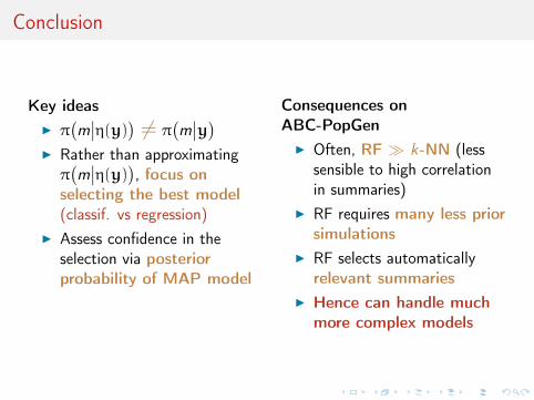
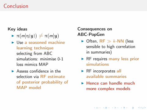
Conclusion
Key ideasI π
(m∣∣η(y)) 6= π
(m∣∣y)
I Rather than approximatingπ(m∣∣η(y)), focus on
selecting the best model(classif. vs regression)
I Assess confidence in theselection via posteriorprobability of MAP model
Consequences onABC-PopGen
I Often, RF � k-NN (lesssensible to high correlationin summaries)
I RF requires many less priorsimulations
I RF selects automaticallyrelevant summaries
I Hence can handle muchmore complex models
Conclusion
Key ideasI π
(m∣∣η(y)) 6= π
(m∣∣y)
I Use a seasoned machinelearning techniqueselecting from ABCsimulations: minimise 0-1loss mimics MAP
I Assess confidence in theselection via RF estimateof posterior probability ofMAP model
Consequences onABC-PopGen
I Often, RF � k-NN (lesssensible to high correlationin summaries)
I RF requires many less priorsimulations
I RF incorporates allavailable summaries
I Hence can handle muchmore complex models
Further features
I unlimited aggregation of arbitrary summary statisticsI recovery of discriminant statistics when availableI automated implementation with reduced calibrationI self-evaluation by posterior predictive error probabilityI soon to appear in DIYABC
Recommended


![Approximate Bayesian Computation for Granular and ...€¦ · reaction networks [24]. To remedy this, the Approximate Bayesian Computation (ABC) [24, 29] framework was intro-duced](https://img.pdfslide.us/doc/110x75/5ff8093d84f1a843b140a517/approximate-bayesian-computation-for-granular-and-reaction-networks-24-to.jpg)