Applied Mathematics 225
Unit 3: Finite element methods
Lecturer: Chris H. Rycroft
Finite element methods
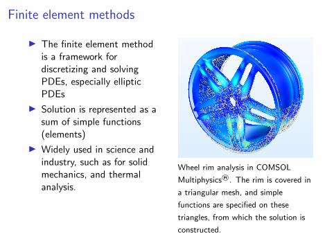
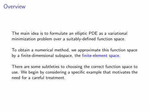
I The finite element methodis a framework fordiscretizing and solvingPDEs, especially ellipticPDEs
I Solution is represented as asum of simple functions(elements)
I Widely used in science andindustry, such as for solidmechanics, and thermalanalysis.
Wheel rim analysis in COMSOL
Multiphysics®. The rim is covered in
a triangular mesh, and simple
functions are specified on these
triangles, from which the solution is
constructed.
Comparison with finite-difference methods
Finite element methods
I make it easier to deal with complex boundary conditions,
I provide more mathematical guarantees about convergence.
Finite difference methods
I are simpler to implement, and sometimes more efficient forthe same level of accuracy,
I are easier to apply to a wider range of equations(e.g. hyperbolic equations).
These are just broad generalizations though—both methods have alarge body of literature, with many extensions.
Frequently, the two approaches lead to similar1 numericalimplementations.
1And in some cases identical.
Book references
We will make use of the following books:
I Claes Johnson. Numerical Solution of Partial DifferentialEquations by the Finite Element Method. Dover, 2009.2
I Thomas J. R. Hughes. The Finite Element Method: LinearStatic and Dynamic Finite Element Analysis. Dover, 2000.3
I Dietrich Braess, Finite elements: Theory, fast solvers, andapplications in solid mechanics, Cambridge University Press,2007.4
2A good general introduction.3Comprehensive, with a particular emphasis on solid mechanics.4A more technically rigorous treatment of the subject.
Overview
The main idea is to formulate an elliptic PDE as a variationalminimization problem over a suitably-defined function space.
To obtain a numerical method, we approximate this function spaceby a finite-dimensional subspace, the finite-element space.
There are some subtleties to choosing the correct function space touse. We begin by considering a specific example that motivates theneed for a careful treatment.
The need for a careful treatment
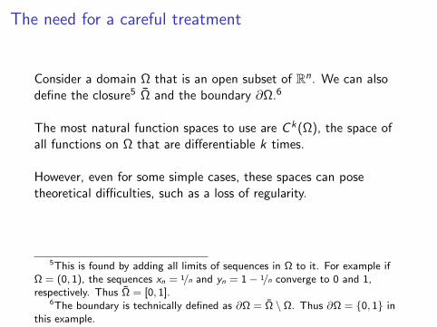
Consider a domain Ω that is an open subset of Rn. We can alsodefine the closure5 Ω and the boundary ∂Ω.6
The most natural function spaces to use are C k(Ω), the space ofall functions on Ω that are differentiable k times.
However, even for some simple cases, these spaces can posetheoretical difficulties, such as a loss of regularity.
5This is found by adding all limits of sequences in Ω to it. For example ifΩ = (0, 1), the sequences xn = 1/n and yn = 1− 1/n converge to 0 and 1,respectively. Thus Ω = [0, 1].
6The boundary is technically defined as ∂Ω = Ω \ Ω. Thus ∂Ω = 0, 1 inthis example.
The need for a careful treatment
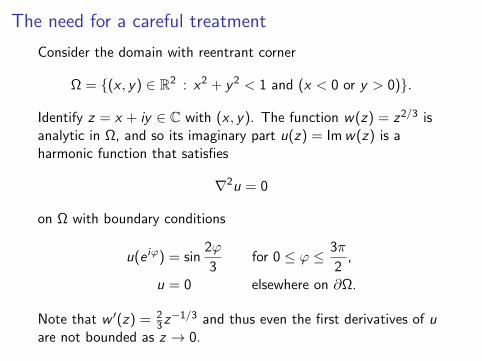
Consider the domain with reentrant corner
Ω = (x , y) ∈ R2 : x2 + y2 < 1 and (x < 0 or y > 0).
Identify z = x + iy ∈ C with (x , y). The function w(z) = z2/3 isanalytic in Ω, and so its imaginary part u(z) = Imw(z) is aharmonic function that satisfies
∇2u = 0
on Ω with boundary conditions
u(e iϕ) = sin2ϕ
3for 0 ≤ ϕ ≤ 3π
2,
u = 0 elsewhere on ∂Ω.
Note that w ′(z) = 23z−1/3 and thus even the first derivatives of u
are not bounded as z → 0.
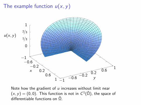
The example function u(x , y)
−1−0.6−0.2
0.20.6
1 −1−0.6
−0.20.2
0.61
0
1/3
2/3
1
x
y
u(x , y)
Note how the gradient of u increases without limit near(x , y) = (0, 0). This function is not in C 1(Ω), the space ofdifferentiable functions on Ω.
The need for a careful treatment
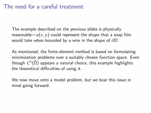
The example described on the previous slides is physicallyreasonable—u(x , y) could represent the shape that a soap filmwould take when bounded by a wire in the shape of ∂Ω.
As mentioned, the finite-element method is based on formulatingminimization problems over a suitably chosen function space. Eventhough C 1(Ω) appears a natural choice, this example highlightsthe theoretical difficulties of using it.
We now move onto a model problem, but we bear this issue inmind going forward.
One-dimensional model problem
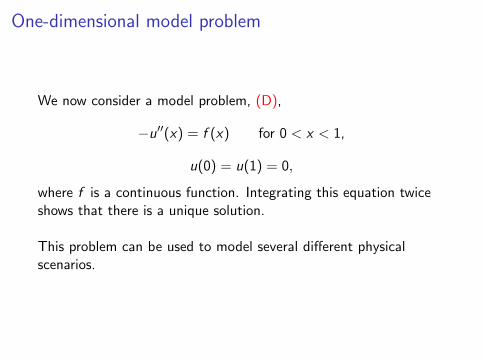
We now consider a model problem, (D),
−u′′(x) = f (x) for 0 < x < 1,
u(0) = u(1) = 0,
where f is a continuous function. Integrating this equation twiceshows that there is a unique solution.
This problem can be used to model several different physicalscenarios.
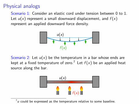
Physical analogsScenario 1: Consider an elastic cord under tension between 0 to 1.Let u(x) represent a small downward displacement, and f (x)represent an applied downward force density.
(x)
u(x)
f
Scenario 2: Let u(x) be the temperature in a bar whose ends arekept at a fixed temperature of zero.7 Let f (x) be an applied heatsource along the bar.
(x)
u(x)
f7u could be expressed as the temperature relative to some baseline.
Alternative formulations
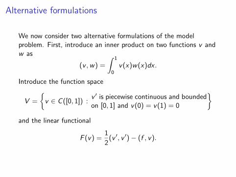
We now consider two alternative formulations of the modelproblem. First, introduce an inner product on two functions v andw as
(v ,w) =
∫ 1
0v(x)w(x)dx .
Introduce the function space
V =
v ∈ C ([0, 1]) :
v ′ is piecewise continuous and boundedon [0, 1] and v(0) = v(1) = 0
and the linear functional
F (v) =1
2(v ′, v ′)− (f , v).
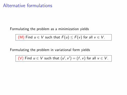
Alternative formulations
Formulating the problem as a minimization yields
(M) Find u ∈ V such that F (u) ≤ F (v) for all v ∈ V .
Formulating the problem in variational form yields
(V) Find u ∈ V such that (u′, v ′) = (f , v) for all v ∈ V .
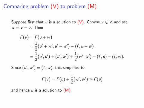
Comparing problem (V) to problem (M)
Suppose first that u is a solution to (V). Choose v ∈ V and setw = v − u. Then
F (v) = F (u + w)
=1
2(u′ + w ′, u′ + w ′)− (f , u + w)
=1
2(u′, u′) + (u′,w ′) +
1
2(w ′,w ′)− (f , u)− (f ,w).
Since (u′,w ′) = (f ,w), this simplifies to
F (v) = F (u) +1
2(w ′,w ′) ≥ F (u)
and hence u is a solution to (M).
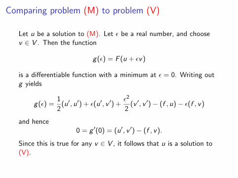
Comparing problem (M) to problem (V)
Let u be a solution to (M). Let ε be a real number, and choosev ∈ V . Then the function
g(ε) = F (u + εv)
is a differentiable function with a minimum at ε = 0. Writing outg yields
g(ε) =1
2(u′, u′) + ε(u′, v ′) +
ε2
2(v ′, v ′)− (f , u)− ε(f , v)
and hence0 = g ′(0) = (u′, v ′)− (f , v).
Since this is true for any v ∈ V , it follows that u is a solution to(V).
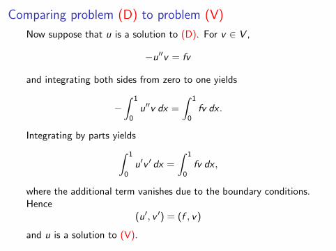
Comparing problem (D) to problem (V)
Now suppose that u is a solution to (D). For v ∈ V ,
−u′′v = fv
and integrating both sides from zero to one yields
−∫ 1
0u′′v dx =
∫ 1
0fv dx .
Integrating by parts yields∫ 1
0u′v ′ dx =
∫ 1
0fv dx ,
where the additional term vanishes due to the boundary conditions.Hence
(u′, v ′) = (f , v)
and u is a solution to (V).
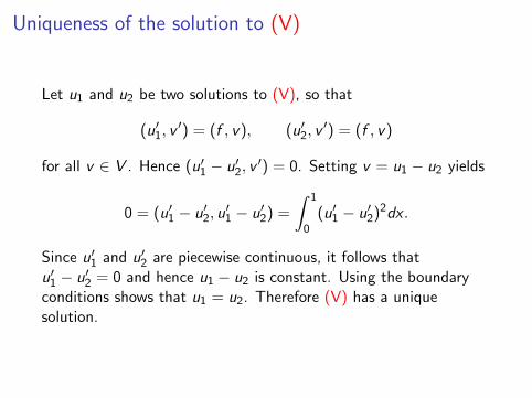
Uniqueness of the solution to (V)
Let u1 and u2 be two solutions to (V), so that
(u′1, v′) = (f , v), (u′2, v
′) = (f , v)
for all v ∈ V . Hence (u′1 − u′2, v′) = 0. Setting v = u1 − u2 yields
0 = (u′1 − u′2, u′1 − u′2) =
∫ 1
0(u′1 − u′2)2dx .
Since u′1 and u′2 are piecewise continuous, it follows thatu′1 − u′2 = 0 and hence u1 − u2 is constant. Using the boundaryconditions shows that u1 = u2. Therefore (V) has a uniquesolution.
Summary
We have now shown that
(D) =⇒ (V)⇐⇒ (M).
Does (V) =⇒ (D)? No, since functions in V are only required tohave a piecewise continuous first derivative. They may not have asecond derivative, which is required in order to satisfy (D).
However, if we place additional restrictions on a solution u to (V),then we can obtain a solution to (D).
Comparing problem (V) to problem (D)
Suppose that u ∈ V satisfies (V), and in addition u′′ exists and iscontinuous. Then ∫ 1
0u′v ′ dx =
∫ 1
0fv dx
for all v ∈ V and integrating by parts yields
−∫ 1
0u′′v dx =
∫ 1
0fv dx .
Therefore ∫ 1
0(u′′ + f )v dx = 0
and since this is true for all v ∈ V it follows that −u′′ = f . By theconstruction of V , u satisfies the boundary conditionsu(0) = u(1) = 0, and hence u is a solution to (D).
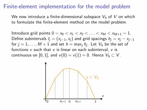
Finite-element implementation for the model problem
We now introduce a finite-dimensional subspace Vh of V on whichto formulate the finite-element method on the model problem.
Introduce grid points 0 = x0 < x1 < x2 < . . . < xM < xM+1 = 1.Define subintervals Ij = (xj−1, xj) and grid spacings hj = xj − xj−1
for j = 1, . . . ,M + 1 and set h = maxj hj . Let Vh be the set offunctions v such that v is linear on each subinterval, v iscontinuous on [0, 1], and v(0) = v(1) = 0. Hence Vh ⊂ V .
x0 1xj xj+1xj 1–
v ∈ Vh
Finite-element implementation for the model problem
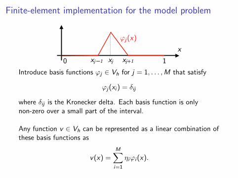
x0 1xj xj+1xj 1–
ϕj(x)
Introduce basis functions ϕj ∈ Vh for j = 1, . . . ,M that satisfy
ϕj(xi ) = δij
where δij is the Kronecker delta. Each basis function is onlynon-zero over a small part of the interval.
Any function v ∈ Vh can be represented as a linear combination ofthese basis functions as
v(x) =M∑i=1
ηiϕi (x).
Finite-element implementation for the model problem
The finite-dimensional equivalent of the minimization problem isthen
(Mh) Find u ∈ Vh such that F (u) ≤ F (v) for all v ∈ Vh.
The finite-dimensional equivalent of the variational problem is
(Vh) Find u ∈ Vh such that (u′, v ′) = (f , v) for all v ∈ Vh.
(Vh) is referred to as Galerkin’s method and (Mh) is referred to asRitz’ method.
Galerkin’s method
Let uh be a solution to (Vh). Then for any basis function ϕj ,
(u′h, ϕ′j) = (f , ϕj).
Write the solution as
uh(x) =M∑i=1
ξiϕi (x).
ThenM∑i=1
ξi (ϕ′i , ϕ′j) = (f , φj),
which is a linear system, Aξ = b, for a vector of unknowns ξ.
Galerkin’s method: matrix formulation
Writing out the matrix problem gives
A =
a11 a12 . . . a1M
a21 a22 . . . a2M...
.... . .
...aM1 aM2 . . . aMM
, ξ =
ξ1
ξ2...ξM
, b =
b1
b2...
bM
,where
aij = (ϕ′i , ϕ′j), bi = (f , ϕi ).
A is called the stiffness matrix and b is the load vector. Thisterminology dates from early work on finite-element methods forstructural mechanics.
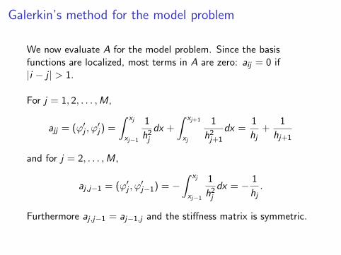
Galerkin’s method for the model problem
We now evaluate A for the model problem. Since the basisfunctions are localized, most terms in A are zero: aij = 0 if|i − j | > 1.
For j = 1, 2, . . . ,M,
ajj = (ϕ′j , ϕ′j) =
∫ xj
xj−1
1
h2j
dx +
∫ xj+1
xj
1
h2j+1
dx =1
hj+
1
hj+1
and for j = 2, . . . ,M,
aj ,j−1 = (ϕ′j , ϕ′j−1) = −
∫ xj
xj−1
1
h2j
dx = − 1
hj.
Furthermore aj ,j−1 = aj−1,j and the stiffness matrix is symmetric.
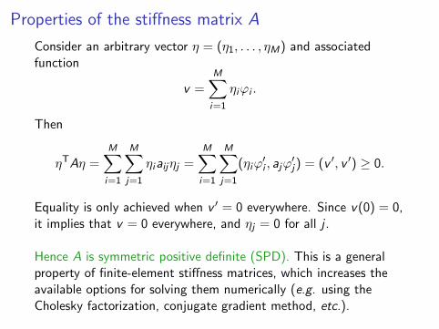
Properties of the stiffness matrix A
Consider an arbitrary vector η = (η1, . . . , ηM) and associatedfunction
v =M∑i=1
ηiϕi .
Then
ηTAη =M∑i=1
M∑j=1
ηiaijηj =M∑i=1
M∑j=1
(ηiϕ′i , ajϕ
′j) = (v ′, v ′) ≥ 0.
Equality is only achieved when v ′ = 0 everywhere. Since v(0) = 0,it implies that v = 0 everywhere, and ηj = 0 for all j .
Hence A is symmetric positive definite (SPD). This is a generalproperty of finite-element stiffness matrices, which increases theavailable options for solving them numerically (e.g. using theCholesky factorization, conjugate gradient method, etc.).
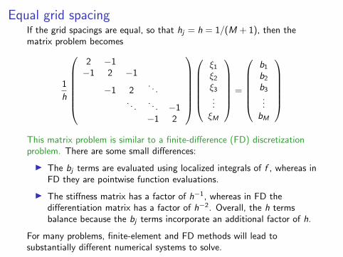
Equal grid spacingIf the grid spacings are equal, so that hj = h = 1/(M + 1), then thematrix problem becomes
1
h
2 −1−1 2 −1
−1 2. . .
. . .. . . −1−1 2
ξ1
ξ2
ξ3
...ξM
=
b1
b2
b3
...bM
This matrix problem is similar to a finite-difference (FD) discretizationproblem. There are some small differences:
I The bj terms are evaluated using localized integrals of f , whereas inFD they are pointwise function evaluations.
I The stiffness matrix has a factor of h−1, whereas in FD thedifferentiation matrix has a factor of h−2. Overall, the h termsbalance because the bj terms incorporate an additional factor of h.
For many problems, finite-element and FD methods will lead tosubstantially different numerical systems to solve.
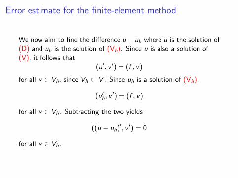
Error estimate for the finite-element method
We now aim to find the difference u− uh where u is the solution of(D) and uh is the solution of (Vh). Since u is also a solution of(V), it follows that
(u′, v ′) = (f , v)
for all v ∈ Vh, since Vh ⊂ V . Since uh is a solution of (Vh),
(u′h, v′) = (f , v)
for all v ∈ Vh. Subtracting the two yields
((u − uh)′, v ′) = 0
for all v ∈ Vh.
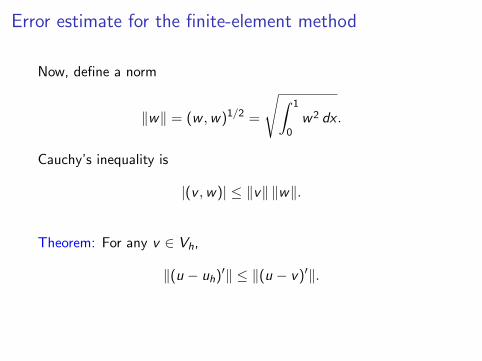
Error estimate for the finite-element method
Now, define a norm
‖w‖ = (w ,w)1/2 =
√∫ 1
0w2 dx .
Cauchy’s inequality is
|(v ,w)| ≤ ‖v‖ ‖w‖.
Theorem: For any v ∈ Vh,
‖(u − uh)′‖ ≤ ‖(u − v)′‖.
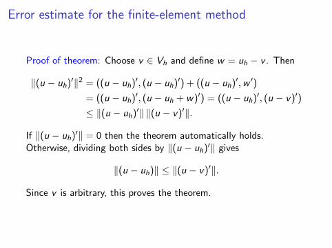
Error estimate for the finite-element method
Proof of theorem: Choose v ∈ Vh and define w = uh − v . Then
‖(u − uh)′‖2 = ((u − uh)′, (u − uh)′) + ((u − uh)′,w ′)
= ((u − uh)′, (u − uh + w)′) = ((u − uh)′, (u − v)′)
≤ ‖(u − uh)′‖ ‖(u − v)′‖.
If ‖(u − uh)′‖ = 0 then the theorem automatically holds.Otherwise, dividing both sides by ‖(u − uh)′‖ gives
‖(u − uh)‖ ≤ ‖(u − v)′‖.
Since v is arbitrary, this proves the theorem.
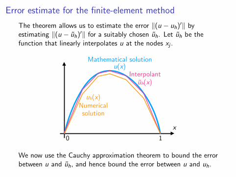
Error estimate for the finite-element method
The theorem allows us to estimate the error ‖(u − uh)′‖ byestimating ‖(u − uh)′‖ for a suitably chosen uh. Let uh be thefunction that linearly interpolates u at the nodes xj .
x0 1
u(x)
uh(x)˜
uh(x)
Mathematical solution
Interpolant
Numerical solution
We now use the Cauchy approximation theorem to bound the errorbetween u and uh, and hence bound the error between u and uh.
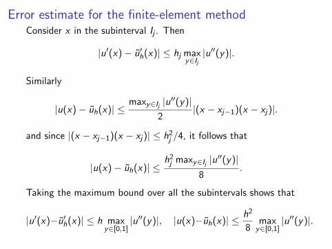
Error estimate for the finite-element methodConsider x in the subinterval Ij . Then
|u′(x)− u′h(x)| ≤ hj maxy∈Ij|u′′(y)|.
Similarly
|u(x)− uh(x)| ≤maxy∈Ij |u′′(y)|
2|(x − xj−1)(x − xj)|.
and since |(x − xj−1)(x − xj)| ≤ h2j /4, it follows that
|u(x)− uh(x)| ≤h2j maxy∈Ij |u′′(y)|
8.
Taking the maximum bound over all the subintervals shows that
|u′(x)−u′h(x)| ≤ h maxy∈[0,1]
|u′′(y)|, |u(x)−uh(x)| ≤ h2
8maxy∈[0,1]
|u′′(y)|.
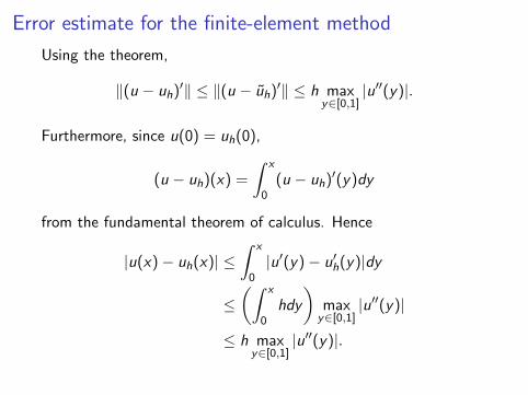
Error estimate for the finite-element method
Using the theorem,
‖(u − uh)′‖ ≤ ‖(u − uh)′‖ ≤ h maxy∈[0,1]
|u′′(y)|.
Furthermore, since u(0) = uh(0),
(u − uh)(x) =
∫ x
0(u − uh)′(y)dy
from the fundamental theorem of calculus. Hence
|u(x)− uh(x)| ≤∫ x
0|u′(y)− u′h(y)|dy
≤(∫ x
0hdy
)maxy∈[0,1]
|u′′(y)|
≤ h maxy∈[0,1]
|u′′(y)|.
Error estimate for the finite-element method
These bounds show that as the grid spacing h decreases, thenumerical solution uh will converge to the mathematical solution u.
The derivation of the bounds shows that the error scales like O(h),which is sufficient to establish convergence.
However, using a more detailed derivation, it is possible to showthat the error scales like O(h2) for this model problem.
Appropriate function spaces for variational problems
In the model problem considered so far, we searched for solutionsover the function space
V =
v ∈ C ([0, 1]) :
v ′ is piecewise continuous and boundedon [0, 1] and v(0) = v(1) = 0
.
However, for mathematical analysis it is advantageous to work witha slightly larger space of functions. The condition about requiringa piecewise continuous derivative is stricter than necessary.
We find that it is appropriate to work with Hilbert spaces, whichhave three requirements detailed on the following slides.
(1) Hilbert spaces are vector spaces
A Hilbert space V is a vector space. It must satisfy basicproperties of commutatativity, associativity, and distributivity.8
We focus on real vector spaces,9 where scalar multiplication isdone using elements of R.
A key property of a real vector space is linearity, so that for anyα, β ∈ R and v ,w ∈ V , the element
αv + βw
is also in V .
8See Wolfram MathWorld or Wikipedia for complete details.9There are also, e.g., complex vector spaces where scalar multiplication is
done using elements of C.
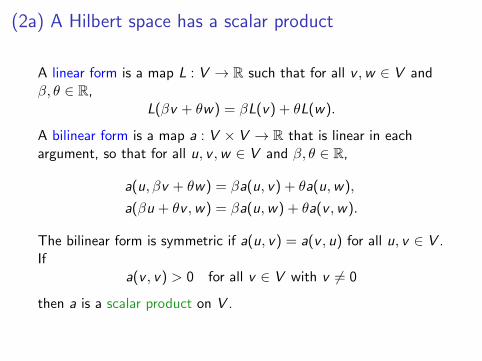
(2a) A Hilbert space has a scalar product
A linear form is a map L : V → R such that for all v ,w ∈ V andβ, θ ∈ R,
L(βv + θw) = βL(v) + θL(w).
A bilinear form is a map a : V × V → R that is linear in eachargument, so that for all u, v ,w ∈ V and β, θ ∈ R,
a(u, βv + θw) = βa(u, v) + θa(u,w),
a(βu + θv ,w) = βa(u,w) + θa(v ,w).
The bilinear form is symmetric if a(u, v) = a(v , u) for all u, v ∈ V .If
a(v , v) > 0 for all v ∈ V with v 6= 0
then a is a scalar product on V .
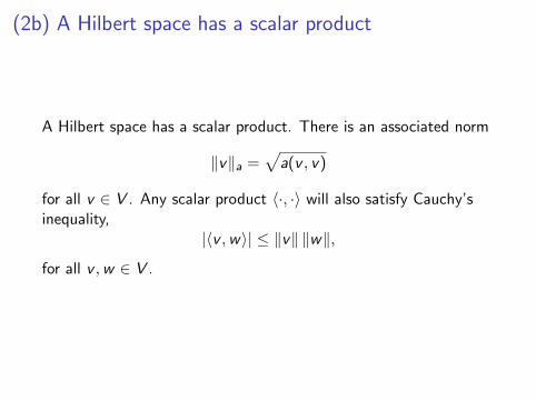
(2b) A Hilbert space has a scalar product
A Hilbert space has a scalar product. There is an associated norm
‖v‖a =√
a(v , v)
for all v ∈ V . Any scalar product 〈·, ·〉 will also satisfy Cauchy’sinequality,
|〈v ,w〉| ≤ ‖v‖ ‖w‖,
for all v ,w ∈ V .
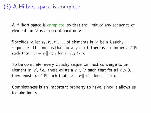
(3) A Hilbert space is complete
A Hilbert space is complete, so that the limit of any sequence ofelements in V is also contained in V .
Specifically, let v1, v2, v3, . . . of elements in V be a Cauchysequence. This means that for any ε > 0 there is a number n ∈ Nsuch that ‖vi − vj‖ < ε for all i , j > n.
To be complete, every Cauchy sequence must converge to anelement in V , i.e., there exists a v ∈ V such that for all ε > 0,there exists m ∈ N such that ‖v − vi‖ < ε for all i > m.
Completeness is an important property to have, since it allows usto take limits.
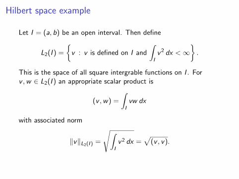
Hilbert space example
Let I = (a, b) be an open interval. Then define
L2(I ) =
v : v is defined on I and
∫Iv2 dx <∞
.
This is the space of all square intergrable functions on I . Forv ,w ∈ L2(I ) an appropriate scalar product is
(v ,w) =
∫Ivw dx
with associated norm
‖v‖L2(I ) =
√∫Iv2 dx =
√(v , v).
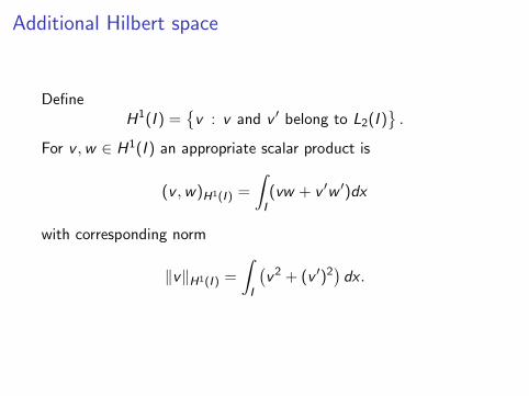
Additional Hilbert space
DefineH1(I ) =
v : v and v ′ belong to L2(I )
.
For v ,w ∈ H1(I ) an appropriate scalar product is
(v ,w)H1(I ) =
∫I(vw + v ′w ′)dx
with corresponding norm
‖v‖H1(I ) =
∫I
(v2 + (v ′)2
)dx .
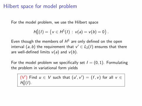
Hilbert space for model problem
For the model problem, we use the Hilbert space
H10 (I ) =
v ∈ H1(I ) : v(a) = v(b) = 0
.
Even though the members of H1 are only defined on the openinterval (a, b) the requirement that v ′ ∈ L2(I ) ensures that thereare well-defined limits v(a) and v(b).
For the model problem we specifically set I = (0, 1). Formulatingthe problem in variational form yields
(V′) Find u ∈ V such that (u′, v ′) = (f , v) for all v ∈H1
0 (I ).
Benefits of the weak formulation
The space H10 (I ) is larger than the original space V that was
considered. H10 (I ) is specifically tailored to the variational problem,
and is the largest space on which the variational problem can beformulated.
Working with H10 (I ) is frequently useful for proving the existence of
solutions.
Furthermore, error estimates are often more natural in the H1(I )norm that incorporates derivative information.
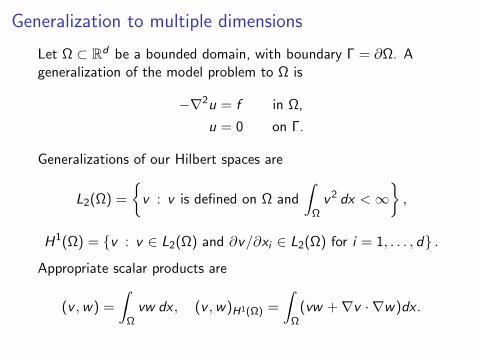
Generalization to multiple dimensions
Let Ω ⊂ Rd be a bounded domain, with boundary Γ = ∂Ω. Ageneralization of the model problem to Ω is
−∇2u = f in Ω,
u = 0 on Γ.
Generalizations of our Hilbert spaces are
L2(Ω) =
v : v is defined on Ω and
∫Ωv2 dx <∞
,
H1(Ω) = v : v ∈ L2(Ω) and ∂v/∂xi ∈ L2(Ω) for i = 1, . . . , d .
Appropriate scalar products are
(v ,w) =
∫Ωvw dx , (v ,w)H1(Ω) =
∫Ω
(vw +∇v · ∇w)dx .
Generalization to multiple dimensions
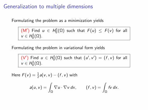
Formulating the problem as a minimization yields
(M′) Find u ∈ H10 (Ω) such that F (u) ≤ F (v) for all
v ∈ H10 (Ω).
Formulating the problem in variational form yields
(V′) Find u ∈ H10 (Ω) such that (u′, v ′) = (f , v) for all
v ∈ H10 (Ω).
Here F (v) = 12a(v , v)− (f , v) with
a(u, v) =
∫Ω∇u · ∇v dx , (f , v) =
∫Ωfv dx .
Neumann boundary conditions
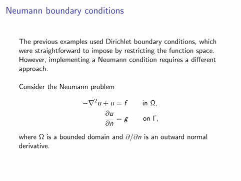
The previous examples used Dirichlet boundary conditions, whichwere straightforward to impose by restricting the function space.However, implementing a Neumann condition requires a differentapproach.
Consider the Neumann problem
−∇2u + u = f in Ω,
∂u
∂n= g on Γ,
where Ω is a bounded domain and ∂/∂n is an outward normalderivative.
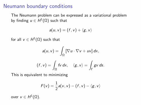
Neumann boundary conditions
The Neumann problem can be expressed as a variational problemby finding u ∈ H1(Ω) such that
a(u, v) = (f , v) + 〈g , v〉
for all v ∈ H1(Ω) such that
a(u, v) =
∫Ω
[∇u · ∇v + uv ] dx ,
(f , v) =
∫Ωfv dx , 〈g , v〉 =
∫Γgv ds.
This is equivalent to minimizing
F (v) =1
2a(v , v)− (f , v)− 〈g , v〉
over v ∈ H1(Ω).
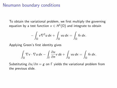
Neumann boundary conditions
To obtain the variational problem, we first multiply the governingequation by a test function v ∈ H1(Ω) and integrate to obtain
−∫
Ωv∇2u dx +
∫Ωvu dx =
∫Ωfv dx .
Applying Green’s first identity gives∫Ω∇v · ∇u dx −
∫Γ
∂u
∂nv ds +
∫Ωvu dx =
∫Ωfv dx .
Substituting ∂u/∂n = g on Γ yields the variational problem fromthe previous slide.
Boundary conditions
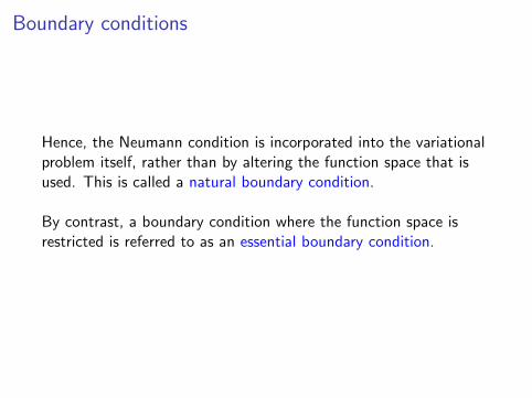
Hence, the Neumann condition is incorporated into the variationalproblem itself, rather than by altering the function space that isused. This is called a natural boundary condition.
By contrast, a boundary condition where the function space isrestricted is referred to as an essential boundary condition.
Example problem
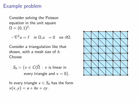
Consider solving the Poissonequation in the unit squareΩ = (0, 1)2:
−∇2u = f in Ω,u = 0 on ∂Ω.
Consider a triangulation like thatshown, with a mesh size of h.Choose
Sh = v ∈ C (Ω : v is linear in
every triangle and v = 0.
In every triangle v ∈ Sh has the formv(x , y) = a + bx + cy .
Example problem
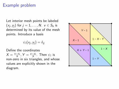
Let interior mesh points be labeled(xj , yj) for j = 1, . . . ,N. v ∈ Sh isdetermined by its value of the meshpoints. Introduce a basis
ψi (xj , yj) = δij
Define the coordinatesX = x−xi
h ,Y = y−yih . Then ψi is
non-zero in six triangles, and whosevalues are explicitly shown in thediagram.
1 – X – Y
1 – X
1 – Y
X + Y – 1
X – 1
Y – 1
Finite-element stencil
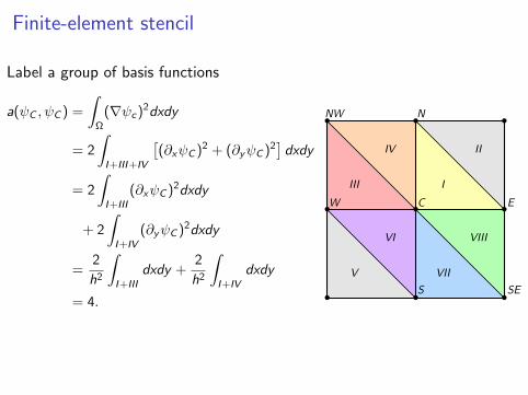
Label a group of basis functions
a(ψC , ψC ) =
∫Ω
(∇ψc)2dxdy
= 2
∫I+III+IV
[(∂xψC )2 + (∂yψC )2
]dxdy
= 2
∫I+III
(∂xψC )2dxdy
+ 2
∫I+IV
(∂yψC )2dxdy
=2
h2
∫I+III
dxdy +2
h2
∫I+IV
dxdy
= 4.
C
S
N
EW
NW
SE
IV II
III I
VI VIII
V VII
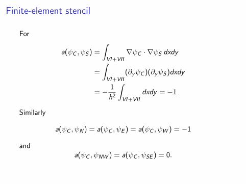
Finite-element stencil
For
a(ψC , ψS) =
∫VI+VII
∇ψC · ∇ψS dxdy
=
∫VI+VII
(∂yψC )(∂yψS)dxdy
= − 1
h2
∫VI+VII
dxdy = −1
Similarly
a(ψC , ψN) = a(ψC , ψE ) = a(ψC , ψW ) = −1
anda(ψC , ψNW ) = a(ψC , ψSE ) = 0.
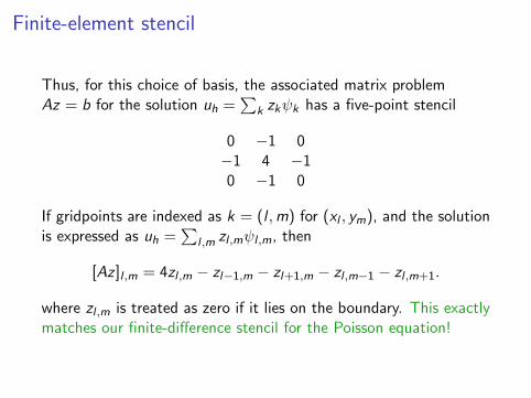
Finite-element stencil
Thus, for this choice of basis, the associated matrix problemAz = b for the solution uh =
∑k zkψk has a five-point stencil
0 −1 0−1 4 −10 −1 0
If gridpoints are indexed as k = (l ,m) for (xl , ym), and the solutionis expressed as uh =
∑l ,m zl ,mψl ,m, then
[Az ]l ,m = 4zl ,m − zl−1,m − zl+1,m − zl ,m−1 − zl ,m+1.
where zl ,m is treated as zero if it lies on the boundary. This exactlymatches our finite-difference stencil for the Poisson equation!
Finite-element stencil
Hence, for this choice of basis, the finite-element (FE) method andthe finite-difference (FD) stencil agree. This is not true in general,but highlights the similarities between the two discretizationapproaches.
Note that the treatment of the source term may differ between FEand FD. In FD, we discretize the field f at gridpoints (l ,m) andwrite
[Az ]l ,m = h2fl ,m
In FE, we have the freedom to specify how f is represented, whichaffects the 〈l , ψk〉 terms appearing in the Ritz–Galerkin method.
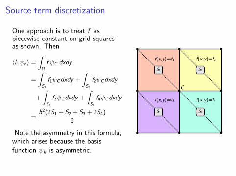
Source term discretization
One approach is to treat f aspiecewise constant on grid squaresas shown. Then
〈l , ψc〉 =
∫Ω
f ψC dxdy
=
∫S1
f1ψCdxdy +
∫S2
f2ψCdxdy
+
∫S3
f3ψCdxdy +
∫S4
f4ψCdxdy
=h2(2S1 + S2 + S3 + 2S4)
6
Note the asymmetry in this formula,which arises because the basisfunction ψk is asymmetric.
S1 S2
S4S3
C
f(x,y)=f2f(x,y)=f1
f(x,y)=f3 f(x,y)=f4
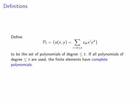
Definitions
DefinePt = u(x , y) =
∑i+k≤t
cikxiyk
to be the set of polynomials of degree ≤ t. If all polynomials ofdegree ≤ t are used, the finite elements have completepolynomials.
Definitions
A finite element is said to be a C k element if it is contained inC k(Ω). Note that the lecture 12 example using right-angledtriangles has C 0 elements.
We use the terminology conforming finite element if the functionslie in the Sobolev space in which the variational problem is posed.
Sometimes, nonconforming elements can be useful, e.g. toapproximate a curved domain with a triangular mesh.
Requirements on the meshes
A partition T = T1,T2, . . . ,TM of Ω into elements is calledadmissible if
1. Ω =⋃M
i=1 Ti .
2. If Ti ∩ Tj consists of exactly one point, it is a common vertexof Ti and Tj .
3. For i 6= j , if Ti ∩ Tj consists of most than one point, thenTi ∩ Tj is a common edge of Ti and Tj .
Properties of the mesh
We write Th instead of T when every element has diameter atmost 2h.
A family of partitions Th is called shape regular provided thatthere exists a number κ > 0 such that every T in Th contains acircle of radius ρT with ρT ≥ hT/κ.A family of partitions Th is called uniform if there exists anumber κ > 0 such that every element T in Th contains a circlewith radius ρT ≥ h/κ.
Differentiability properties
In the one-dimensional finite element example, we used a piecewisecubic that was continuous but not differentiable.
Theorem (see Braess): Let k ≥ 1 and suppose Ω is bounded. Thena piecewise infinitely differentiable function v : Ω→ R belongs toHk(Ω) if and only if v ∈ C k−1(Ω).
Thus functions in C 0 are in H1. For second-order elliptic PDEsthis allows us to calculate the finite element terms a(ψk , ψi ), sinceit involves integrals of weak derivatives ∂ψk .
Fourth-order elliptic problems involve integrals of ∂2ψk andtherefore require C 1 basis functions.
Triangular elements
Any triangle can be transformed into another via an affinetransformation x 7→ Ax + x0 for a matrix A and vector b.
Suppose u is a polynomial of degree t (i.e. a member of Pt). If weapply an affine transformation to u we get another polynomial ofdegree t. Hence Pt is invariant under affine linear transformations.
We therefore look for different ways to represent polynomials ontriangles, from finite element basis functions can be constructed.
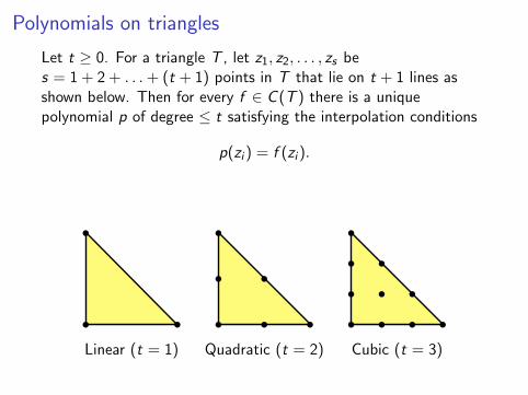
Polynomials on triangles
Let t ≥ 0. For a triangle T , let z1, z2, . . . , zs bes = 1 + 2 + . . .+ (t + 1) points in T that lie on t + 1 lines asshown below. Then for every f ∈ C (T ) there is a uniquepolynomial p of degree ≤ t satisfying the interpolation conditions
p(zi ) = f (zi ).
Linear (t = 1) Quadratic (t = 2) Cubic (t = 3)
Nodal basis
Suppose that for a given finite element space, there is a set ofpoints such that the function values at those points uniquelydetermine the function. Then the set of points is called a nodalbasis.
Suppose we are given a triangulation of Ω and we place points ineach triangle as shown on the previous slide. Points on edges willbe common between triangles. Consider a nodal basis made fromthese points.
Consider two adjacent triangles. The function in each triangle is inPt . The restriction of the function from either side to the commonedge is a polynomial of degree t. Since the restrictions must agreeat the n + 1 nodes along the edge, it follows that the overallfunction is continuous. Thus we have a C 0 nodal basis.10
10The finite element example problem uses a one-dimensional version of thisbasis construction, for the case of cubic elements.
Construction of C 1 elements
Note the nodal basis construction procedure does not lead to C 1
elements, even for t = 2 or t = 3. The basis functions are onlycontinuous across the edges between triangles.
As shown in the finite element example problem, using C 0
elements can still provide high-order accuracy solutions.
Constructing C 1 elements is more difficult. We provide twoexamples.
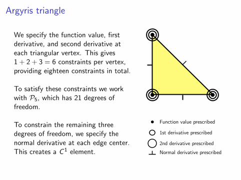
Argyris triangle
We specify the function value, firstderivative, and second derivative ateach triangular vertex. This gives1 + 2 + 3 = 6 constraints per vertex,providing eighteen constraints in total.
To satisfy these constraints we workwith P5, which has 21 degrees offreedom.
To constrain the remaining threedegrees of freedom, we specify thenormal derivative at each edge center.This creates a C 1 element.
Function value prescribed
1st derivative prescribed
2nd derivative prescribedNormal derivative prescribed
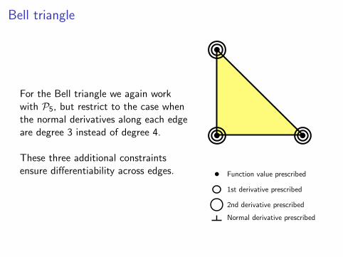
Bell triangle
For the Bell triangle we again workwith P5, but restrict to the case whenthe normal derivatives along each edgeare degree 3 instead of degree 4.
These three additional constraintsensure differentiability across edges. Function value prescribed
1st derivative prescribed
2nd derivative prescribedNormal derivative prescribed
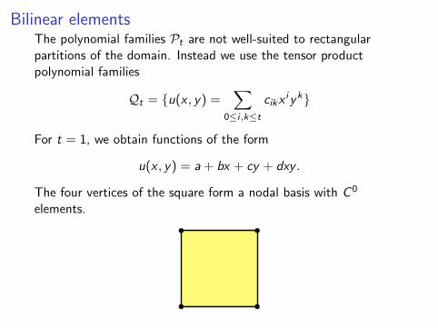
Bilinear elementsThe polynomial families Pt are not well-suited to rectangularpartitions of the domain. Instead we use the tensor productpolynomial families
Qt = u(x , y) =∑
0≤i ,k≤tcikx
iyk
For t = 1, we obtain functions of the form
u(x , y) = a + bx + cy + dxy .
The four vertices of the square form a nodal basis with C 0
elements.
Finite element definition
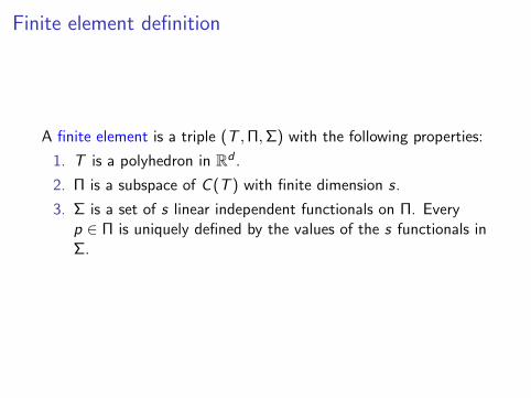
A finite element is a triple (T ,Π,Σ) with the following properties:
1. T is a polyhedron in Rd .
2. Π is a subspace of C (T ) with finite dimension s.
3. Σ is a set of s linear independent functionals on Π. Everyp ∈ Π is uniquely defined by the values of the s functionals inΣ.
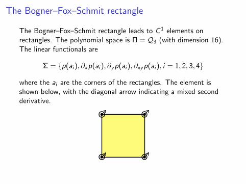
The Bogner–Fox–Schmit rectangle
The Bogner–Fox–Schmit rectangle leads to C 1 elements onrectangles. The polynomial space is Π = Q3 (with dimension 16).The linear functionals are
Σ = p(ai ), ∂xp(ai ), ∂yp(ai ), ∂xyp(ai ), i = 1, 2, 3, 4
where the ai are the corners of the rectangles. The element isshown below, with the diagonal arrow indicating a mixed secondderivative.
Affine families
A family of finite element spaces Sh for partitions Th of Ω is calledan affine family if there exists a finite element (Tref,Πref,Σ) calledthe reference element such that
4. For every Tj ∈ Th there exists an affine mappingFj : Tref → Tj such that for every v ∈ Sh its restriction to Tj
has the formv(x) = p(F−1
j x)
with p ∈ Πref.
Recommended


