Report No. FAA·RD·77·60
APPLICATIONS GUIDE PROPAGATION AND INTERFERENCE ANALYSIS
COMPUTER PROGRAMS (0.1 to 20 GHz)
M.E. Johnson and G.D. Gierhart
U.S. DEPARTMENT OF COMMERCE OFFICE OF TELECOMMUNICATIONS
INSTITUTE FOR TELECOMMUNICATION SCIENCES BOULDER, COLORADO 80303
March 1978
Document is available to the public through the National Technical Information Service,
Springfield, Virginia 22151
Prepared for
U.S. DEPARTMENT OF TRANSPORTATION FEDERAL AVIATION ADMINISTRATION
Systems Research & Development Service Washington, D.C. 20590

NOTICE
This document is disseminated under the spo1sorship of
the Department of Transportation in the interest of in
formation exchange. The United States Government assumes
no liability for its contents or use thereof.

1. Report No. 2. Government Accession No.
FAA-RD-77-60
4. Title ond Subtitle
Applications Guide for Propagation and Interference Analysis Computer Programs (0.1 to 20 GHz)
Technical Report Documentation Page
3. Recipient's Cotolog No.
: 5. Report Dole
March 1978 6. Perfor1ning Orgoni zafion Code
1--=----,...,,..-------------------------i 8. Perfor1ning Orgonizofion Report No. 7. Author's)
.M. E. Johnson and G. D. Gierhart 9. Performing Orgoni zofion Nome ond Address
U. S. Department of Commerce Office of Telecommunications Institute for Telecommunication Sciences
10. Work Unit No. (TRAIS)
Boulder, Colorado 80303 13. TypeoiReportondPeriodCovered ~~--~--------~-------------------4
12. Sponsoring Agency Nome ond Address
U. S. Department of Transportation Federal Aviation Administration Systems Research and Development Service Washington, D. C. 20591 .
14. Sponsoring Agency Code
ARD-60 15. Supplementary Notes
Performed for the Spectrum Management Staff, ATS Spectrum Engineering Branch.
16. Abatroct
This report covers ten computer programs useful in estimating the service coverage of radio systems operating in the frequency band from 0.1 to 20 GHz. These programs may be used to obtain a wide variety of computer-generated microfilm plots such as transmission loss versus path length and the desired-to-undesired signal ratio at a receiving location versus the distance separating the desired and undesired trans mitting facilities. Emphasis is placed on the types of outputs available and the input parameter requirements. The propagation model used with these programs is applicable to air/ground, air/air, ground/ satellite, and air/satellite paths. It can also be used for ground-toground paths that are line-of-sight or smooth earth. Detailed information on the propagation models and software involved is not provided. The normal use made of these programs involves a Department of Commerce (DOC) response to a Federal Aviation Administration (FAA) ARD-60 request for computer output and reimbursement to the DOC by the FAA for the associated costs.
17. KeyWords Air/air, air/ground, computer program, DME, earth/satellite, EMC, frequency sharing, ILS, interference, navigation aids, propagation model, TACAN, transmission loss. VOR.
18. Oi sfri bution Statement
Document is available to the public through the National Technical Information Service, Springfield, Virginia 22151
19. Security Clouif. (of this report) 20. Security Clossil. (of this poge) 21. No. of P oges 22. Price
Unclassified Unclassified 184
Form DOT F 1700.7 (8-72l Reproductio,.; of completed page authorized i
!
•'
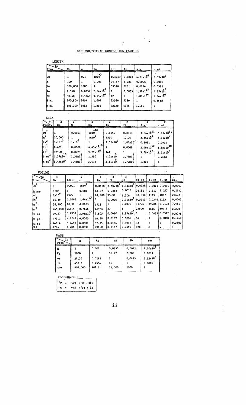
ENGLISH/METRIC CONVERSION FACTORS
LENGTH
,~ Cm m Km in
-5 Cm 1 0,1 1x10 0.3937
ill 100 1 0,001 39.37
l<m 100,000 1000 1 39370
in 2.540 0.0254 -5
2.54x10 1
Itt 30.48 0.3048 3.05x1o" 12
~ mi 160,900 1609 1.609
n mi 185,200 1852 1.852
AREA
~ m
Cm2
,,? Km2
1n2
ft 2
s mt2
n mi 2
VOLUME
~ 1.'1 pm2
iter ~2
3 n
t3
d3
1 oz
1 pt
1 f{t a1
2 2 2 t,;m M K111.
-10 1 0.0001 1x10
10,000 1 b:106
1x10¹⁰ 1x10⁶ 1
6.452 0.0006 -10
6.45x10
929.0 10 0.0929 9.29x10⁸
2.59x1a 2,59x10 2.590
3.43x10° 3.43x18 3.432
3 3 3 Cm Liter m in
1 0.001 1x10° 0.0610
1000 1 0.001 61.02
lx106 1000 1 61,000
0.0163 -5 1 16.39 l.64x10
28,300 28.32 0.02113 1728
765,000 764.5 0.7646 46700 0.2957 -5
29.57 2,96x10 1.805
473.2 0.4732 0.0005 28.88
948.4 0.9463 0.0009 57.75 3785 3.785 0.0038 231.0
MASS
~ g Kg om
g 1 0,001
X& 1000 1
oz 28.35 0.0283
1b 453.6 0.4536
ton 907,000 907.2
TFJfPERATURE 0 1 - 5/9 (oc • 32)
0C • 9/5 (°F) + 32
63360
72930
2 in
0.1550
1550
1.55x10⁹
1
144 9
4.01x10 9
5,31x10
3 ft
3.53x10⁵
0.0353
35.31
0,0006
1
27
0.0010
0.0!67
0.0334 0.133 7
oz
0.0353
35.27
1
16
32,000
ii
ft a mi n mi
0.0328 6.21x10⁶ 5.39x10⁶
3.281 0,0006 0.0005
3281 0.6214 0.5395
0,0833 -5
1.58x10 -5
l.37x10
1 l.89x1o" l.64xlo"
5280 1 0.86,88
6076 1,151 1
2 2 2 ft S m1 nmi
0.0011 3.86xlo11 5.llxl011
10.76 3.86x10⁷ 5.llx10 7
1.08x10⁷ 0.3861 0.2914
0.0069 2.49xl0~0 1.88x10¹⁰
1 3.59xl68 2. 7lx1011
2.79x16 1 o. 7548 7
3, 70x10 1.325 1 i
3 iyd fl oz fl pt f1 qt
-6 1.31xl0 0.0338 0.0021 0.0010
0.0013 33.81 2.113 1.057
1,308 33,800 2113 1057 -5
2.14x10 0.5541 0.0346 2113
0.0370 957.5 59.84 0.0173
1 25900 1616 807.9 -5
3.87xl0 1 0.0625 0.0312
0.0006 16 1 1),5000
0.0012 32 2 1 0.0050 128 8 4
lb ton
0,0022 1.10x1o0
2.205 O,OOll
0.0625 3.12xl05
1 0.0005 2000 1
aa1
0.0002
v.2642
264.2
0,0043
7.481
202.0
0.0078
0.1250
0.2500
1
FEDERAL AVIATION ADMINISTRATION SYSTEMS RESEARCH AND DEVELOPMENT SERVICE
SPECTRUM MA:-.JAGE~1ENT STAFF
Statement of Mission
The mission of the Spectrum Management Staff is to assist the De partment of State, Office of lecommunications Policy, and the Federal Communications Commission in assuring the FAA's and the nation's aviation interests with sufficient protected electromagnetic teleconununications resources throughout the world to provide for the s conduct of aeronautical flight by fostering effective and efficient use of a natural resource- the electromagnetic radio frequency spectrum.
This object is achieved through the following services:
Planning and defending the acquisition and retention of sufficient radio frequency spectrum to support the aeronautical interests of the nation, at home and abroad, and spectrum standardization for the world's aviation community.
Providing research, analysis, engineering, and evaluation in the development of spectrum related policy, planning, standards, criteria, measurement equipment, and measurement techniques.
Conducting electromagnetic compatibility analyses to determine intra/inter-system vjability and design parameters, to assure certification of adequate spectrum to support system operational use and projected growth patterns, to defend aeronaut al services spectrum from encroachment by others, and to provide for the e icient use of the aeronautical spectrum.
Developing automated equency selection computer programs/routines to provide frequency planning, frequency assignment, and spectrum analysis capabilities in the spectrum supporting the National Airspace System.
Providing spectrum management consultation, assistance, and guidance to all aviation interests, users, and providers of equipment and services, both national and international.
Ill

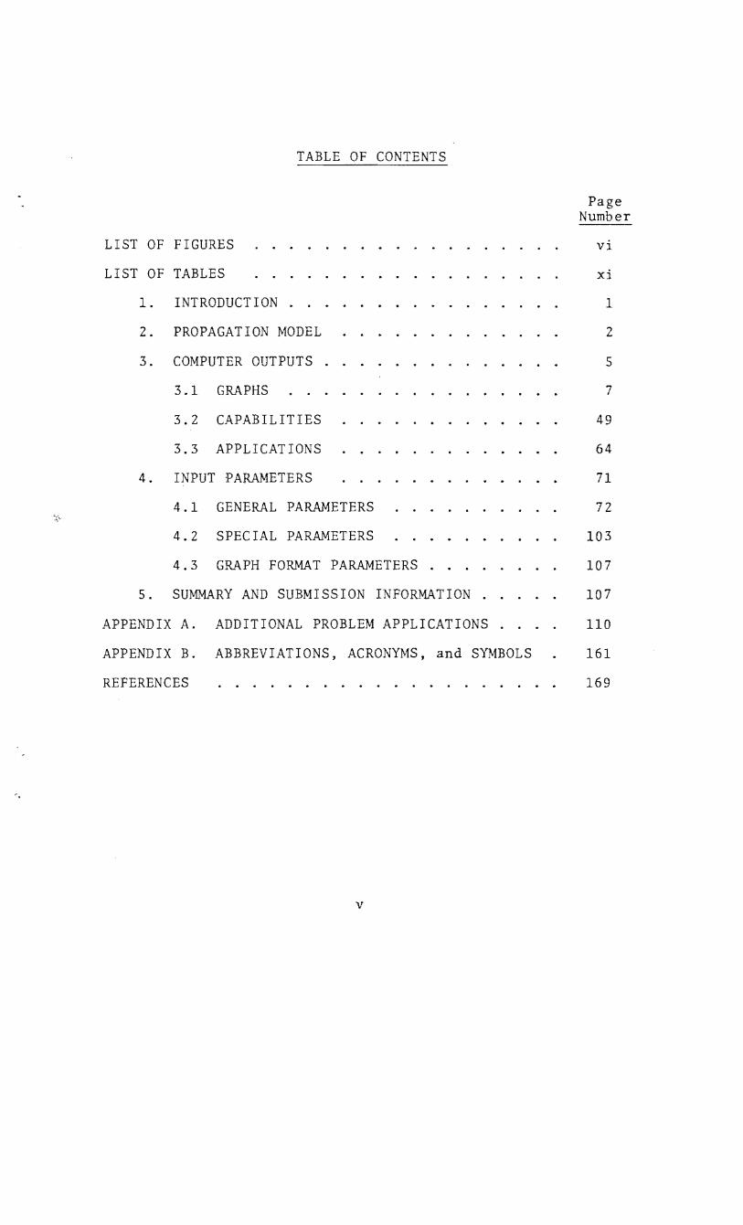
TABLE OF CONTENTS
Page Number
LIST OF FIGURES vi
LIST OF TABLES xi
1. INTRODUCTION . 1
2. PROPAGATION MODEL . . . . . . . 2
3. COMPUTER OUTPUTS . . . 5
3.1 GRAPHS 7
3.2 CAPABILITIES 49
3.3 APPLICATIONS . . . 64
4. INPUT PARAMETERS . . . . . . 71
4.1 GENERAL PARAMETERS . . . 72
4.2 SPECIAL PARAMETERS . . . 103
4.3 GRAPH FORMAT PARAMETERS . . 107
5. SUMMARY AND SUBMISSION INFORMATION . . . . 107
APPENDIX A. ADDITIONAL PROBLEM APPLICATIONS . . . 110
APPENDIX B. ABBREVIATIONS, ACRONYMS, and SYMBOLS 161
REFERENCES . . . . . . . . . . . . . . . . . . . 169
-.
v

Figure Number
LIST OF FIGURES
Caption
1-5 Parameter Sheet,
1
2
3
4
5
6
7
8
9
10
11
12
13
14
15
ATC
ILS
UHF Satellite
TACAN
VOR
Lobing, ATC . . Reflection coefficient, ATC
Path length difference, ATC
Time lag, ATC
Lobing frequency-D, ATC
Lobing frequency-H, ATC
Reflection point, ATC
Elevation angle, ATC .
Elevation angle difference, ATC
Spectral plot, ATC
Page Number
10
11
12
13
14
15
16
17
18
19
20
21
22
23
24
16 Power available, UHF Satellite for sea state 0 25
17-19
17
18
19
20
Power density,
ILS
TACAN
VOR .. Transmission loss, ATC
vi
26
27
28
29
Figure Number
21
22
23
24
25
26
27-29
27
28
29
30
31
32
33
34
35
36-37
36
37
38-39
38
39
40
LIST OF FIGURES (continued)
Power available curves, ATC
Power density curves, ATC
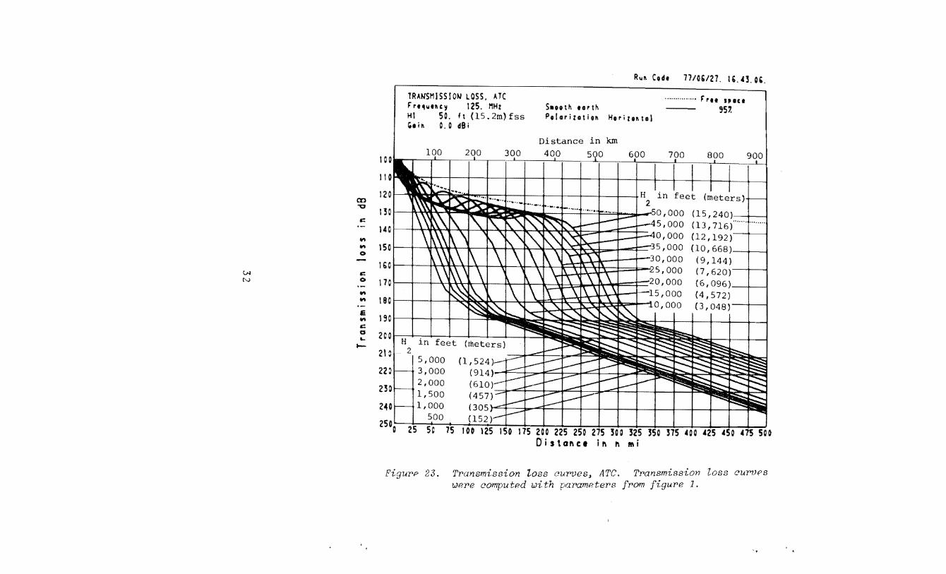
Transmission loss curves, ATC ..
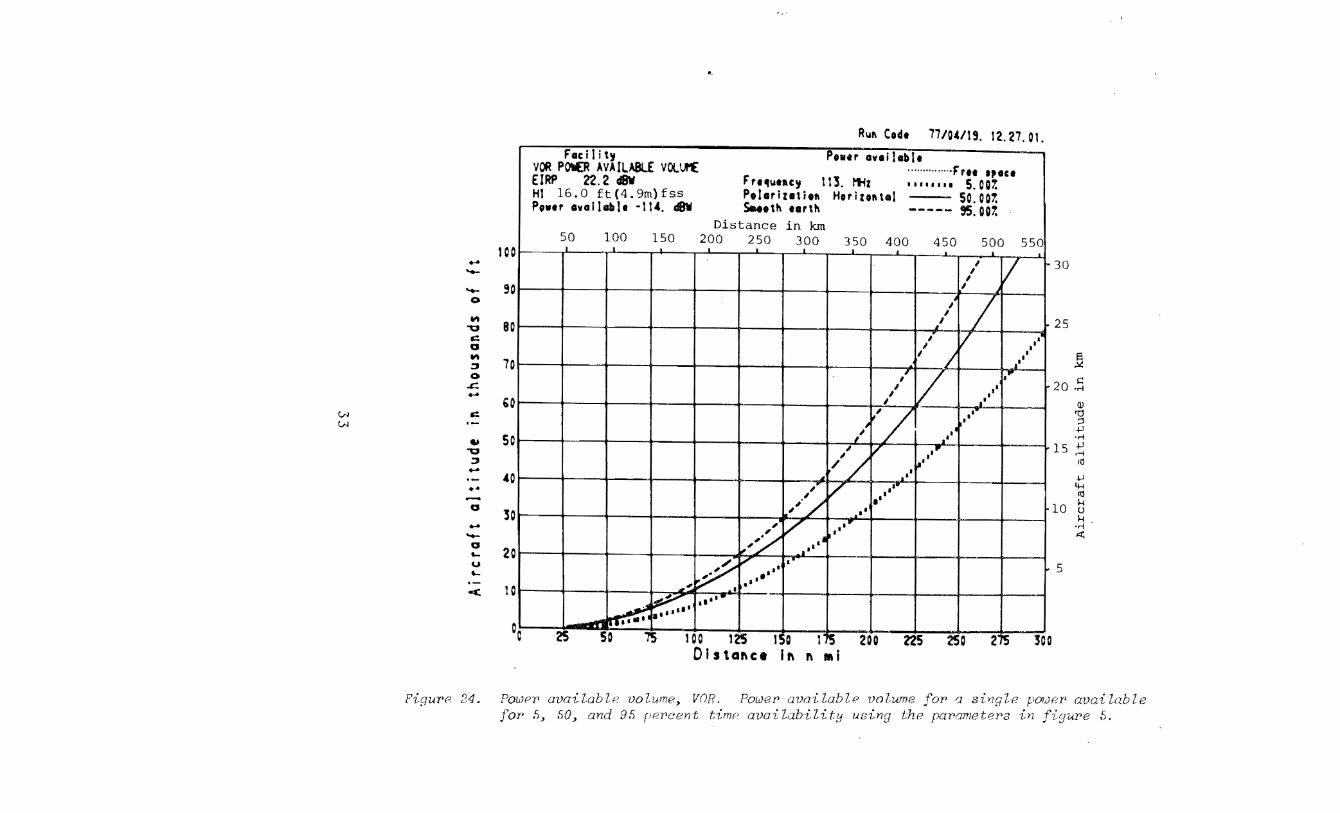
Power available volume, VOR
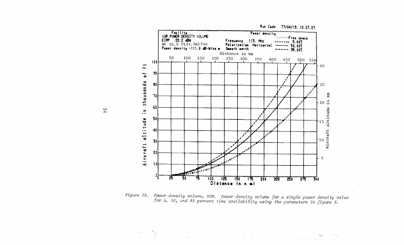
Power density volume, VOR
Transmission loss volume, VOR
EIRP contours,
ILS
TACAN .
VOR .
Power available contours, TACAN
Power density contours, TACAN ..
Transmission loss contours, TACAN
Signal ratio-S, VOR
Signal ratio-DD, VOR
Orientation, ILS
Service volume,
TACAN .
VOR .
ratio contours,
ILS
VOR .
Geometry for reflection from spherical earth
vii
Page Number
30
31
32
33
34
35
36
37
38
39
40
41
42
43
44
45
46
47
48
50
Figure Number
41
LIST OF FIGURES (continued)
Caption
Geometrical location of constant central angle contours . . . . . . . . . . . .
Page Number
55
42 Sketch illustrating interference configuration 60
43 Orientation geometry for protection points 62
44
45
46
47
48
49
50
51
52
53
Al
A2
A3-A8
A3
Antenna heights and surface elevations . . Normalized antenna gain vs. elevation angle
Normalized antenna gain vs. elevation angle, DME . . . . . . . . . . . . . . . .
Signal-level distributions for ionospheric scintillation index groups . . . . . .
Signal-level distributions currently used with variable scintillation group option
.
.
.
.
Rain zones of the Continental United States .
Rain zones of the world . . .
Surface refractivity for the Continental United States . . . . . ...
Surface refractivity of the world .
Contours of the terrain factor ~h in meters
Problem Al, geometry sketch .
Problems Al and A2, parameter sheet, ATC
Transmission loss, ATC,
vertical polarization, lobing option
81
86
87
92
93
95
96
97
98
102
111
112
113
A4 vertical polarization, variability option 114
AS horizontal polarization, lobing option 115
A6 horizontal polarization, variability option . 116
viii
-·
Figure Number
A7
AS
/\9
LIST OF FIGURES (continued)
circular polarization, lobing option
circular polarization, variability option
Problem /\2, geometry sketch
Page Number
117
118
119
AlO-All Transmission loss, 1\TC, vertical polarization,
AlO rolling plains .
All mountains . . . . . .•
Al2 Problem A3, geometry sketch
Al3 Problem A3, parameter sheet, TACAN .
Al4-Al6 Power density, TACAN
Al4
AlS
Al6
Al7
Al8
main lobe at normal elevation
main lobe at 0° elevation
main lobe tracking aircraft
Problems A4 and AS, geometry sketch
Problems A4 and AS, parameter sheet, VHF satellite ..... .
Al9-A21 Power available, VHF satellite,
120
121
122
123
12S
126
127
128
129
scintillation index group 0, sea state 0 Al9 130
scintillation index group s ' sea state 0 A20 131
A21
A22
A23
variable scintillation index group, sea state 0 . . . . . . . . . . . . . .
Problem AS, parameter sheet, UHF satellite
Power available, VHF satellite, scintillation index group 0, sea state 6 .....
A24-A25 Power available, UHF satellite,
A24 scintillation index group 0, sea state 0 ..
ix
132
134
13S
136
Figure Number
A25
A26
LIST OF FIGURES (continued)
Caption
scintillation index group 0, sea state 6
Problem A6, geometry
Page Number
137
138
A27 Problems A6 through A9, parameter sheets, ILS 139
A28 Geometry for S . m1n
A29-A43 Signal ratio-S, ILS,
A29
A30
A31
A32
A33
A34
A35
A36
A37
A38
A39
A40
A41
A42
A43
higher undesired facility elevation .
equal site elevations ..
lower undesired facility elevation
poor ground . .
average ground
good ground
sea water ..
fresh water .
smooth plains .
rolling plains
hills ..
mountains .
extremely rugged mountains
path parameters from topographic maps
path parameters from ECAC terrain file
X
141
142
143
144
146
147
148
149
150
152
153
154
155
156
159
160
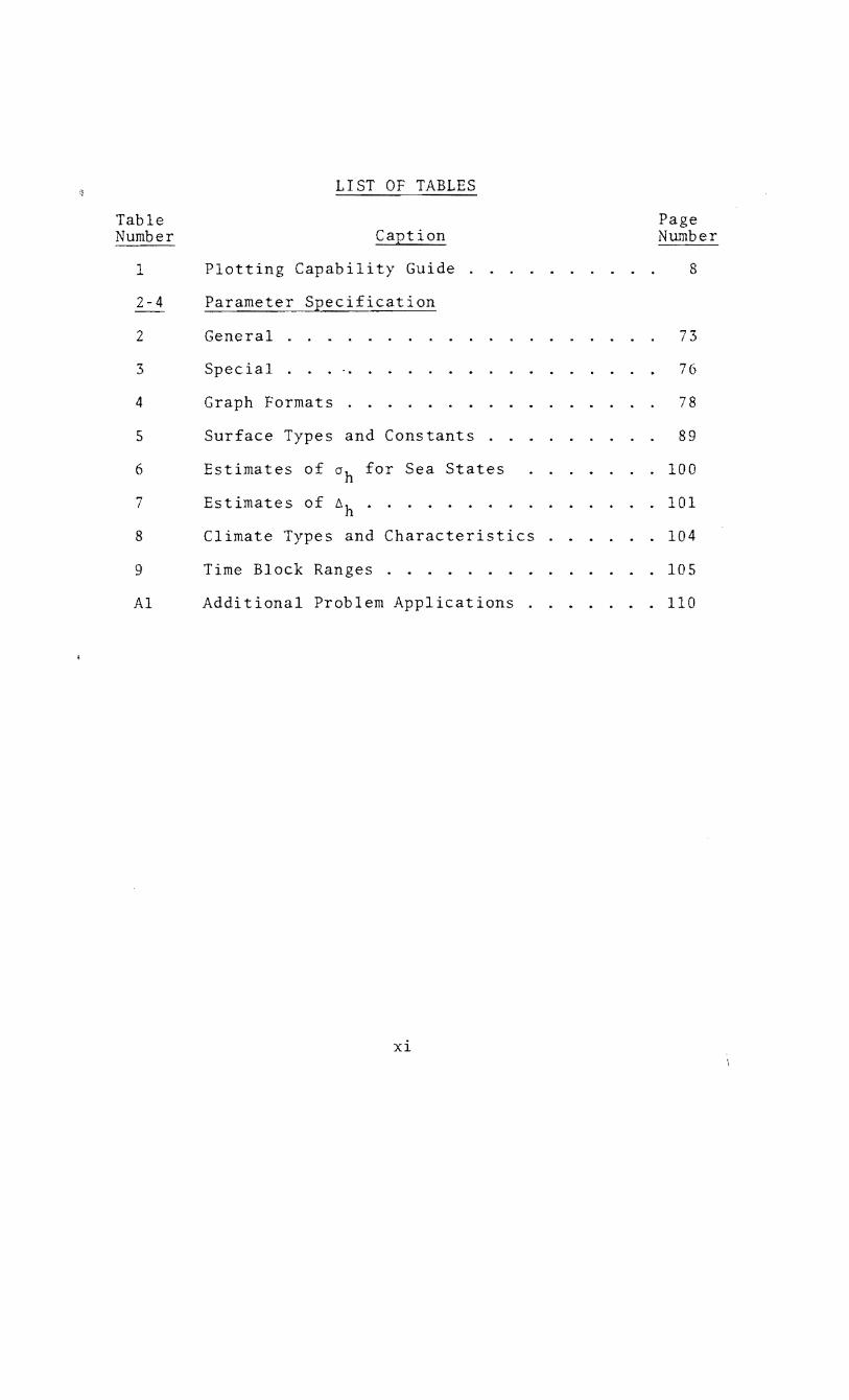
LIST OF TABLES
Table Page Number Ca]2tion Number
1 Plotting Capability Guide . . . . . . . . 8
2-4 Parameter S]2ecification
2 General . . . . 73
3 Special 76
4 Graph Formats 78
5 Surface Types and Constants . 89
6 Estimates of oh for Sea States . 100
7 Estimates of ~h . . . . . 101
8 Climate Types and Characteristics 104
9 Time Block Ranges . . . . . . . 105
Al Additional Problem Applications . . . . 110
xi

xii
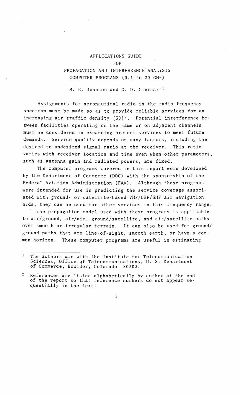
APPLICATIONS GUIDE FOR
PROPAGATION AND INTERFERENCE ANALYSIS COMPUTER PROGRAMS (0.1 to 20 GHz)
M. E. Johnson and G. D. Gierhart 1
Assignments for aeronautical radio in the radio frequency spectrum must be made so as to provide reliable services for an increasing air traffic density [30]2. Potential interference be
tween facilities operating on the same or on adjacent channels
must be considered in expanding present services to meet future demands. Service quality depends on many factors, including the
desired-to-undesired signal ratio at the receiver. This ratio varies with receiver location and time even when other parameters, such as antenna gain and radiated powers, are fixed.
The computer programs cover.ed in this report were developed
by the Department of Commerce (DOC) with the sponsorship of the Federal Aviation Administration (FAA). Although these programs
were intended for use in predicting the service coverage associ
ated with ground- or satellite-based VHF/UHF/SHF air navigation aids, they cari be used for other services in this frequency range.
The propagation model used with these programs is applicable to air/ground, air/air, ground/satellite, and air/satellite paths over smooth or irregular terrain. It can also be used for ground/
ground paths that are line-of-sight, smooth earth, or have a common horizon. These computer programs are useful in estimating
2
The authors are with the Institute for Telecommunication Sciences, Office qf Telecommunications, U. S. Department of Commerce, Boulder, Colorado 80303.
References are listed alphabetically by author at the end of the report so that reference numbers do not appear sequentially in the text~
1

the service coverage of radio systems operating in the frequency
band from about 0.1 to 20 GHz. They may be used to ohtain a wide
variety of computer-generated microfilm plots such as transmis
sion loss [43, 44] versus path length, and the desired-to
undesired signal ratio at a receiving location versus the dis
tance separating the desired and undesired transmitting facili
ties.
This type of information is very similar to that previously developed by DOC during the last decade [19, 20, 21, 22, 23, 24,
26, 27, 32, 38, 39, 49, 55]. The use of such information in spec
trum engineering has been discussed by Hawthorne and Daugherty
[28] and Frisbie et al. [18]; other information on spectrum engineering for air navigation, and communications systems is avail
able [13, 14, 15, 16, 29, 33].
The potential user should
1) read the brief description of the propagation model
provided in section 2 to see it the model could be
applicable to his problem,
2) select the program(s) whose output(s) is most appro
priate from the information provided in section 3,
3) determine values for the input parameters discussed
in section 4, and
4) utilize the information provided in section 5 to re
quest program runs.
Many examples of the graphical output produced by these pro
grams are provided in section 3.1, and additional examples are included in Appendix A (see list of figures). Most abbreviations, acronyms, and symbols used in this report are identified in Ap
pendix B.
2. PROPAGATION MODEL
The DOC has been active in radio wave propagation research and prediction for several decades, and has provided the FAA with
many propagation predictions relevant to the coverage of air
2
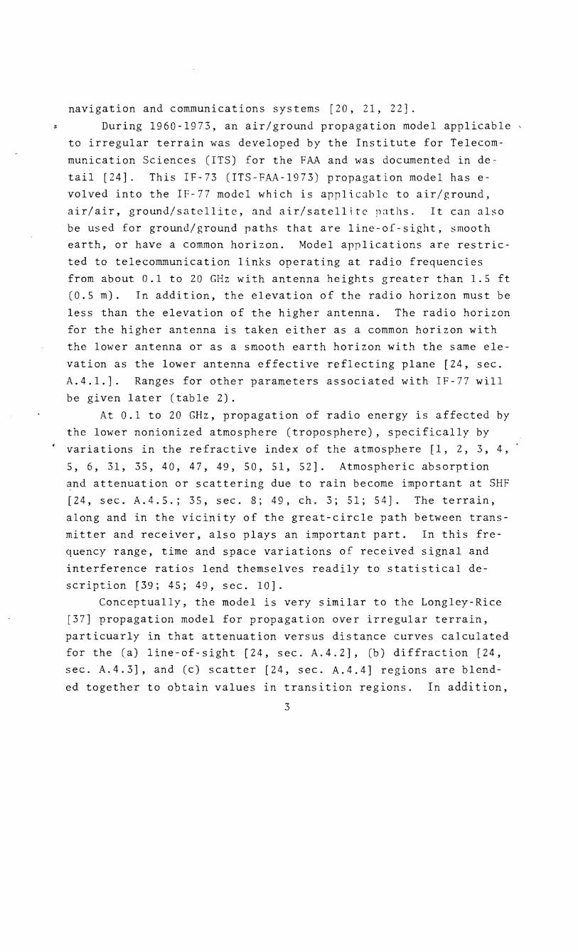
navigation and communications systems [20, 21, 22].
During 1960-1973, an air/ground propagation model applicable
to irregular terrain was developed by the Institute for Telecom
munication Sciences (ITS) for the FAA and was documented in de
tail [24]. This IF-73 (ITS FAA-1973) propagation model has e
volved into the If 77 model which is applicable to air/ground,
air/air, ground/satellite, and air/satellite paths. It can also
be used for ground/ground paths that are line-of-sight, smooth
earth, or have a common horizon. Model applications are restric
ted to telecommunication links operating at radio frequencies
from about 0.1 to 20 GHz with antenna heights greater than 1.5 ft
(0.5 m). In addition, the elevation of the radio horizon must be
less than the elevation of the higher antenna. The radio horizon
for the higher antenna is taken either as a common horizon with
the lower antenna or as a smooth earth horizon with the same ele
vation as the lower antenna effective reflecting plane [24, sec.
A.4.1.]. Ranges for other parameters associated with IF-77 will
be given later (table 2).
At 0.1 to 20 GHz, propagation of radio energy is affected by
the lower nonionized atmosphere (troposphere), specifically by
variations in the refractive index of the atmosphere [1, 2, 3, 4,
5, 6, 31, 35, 40, 47, 49, SO, 51, 52]. Atmospheric absorption
and attenuation or scattering due to rain become important at SHF
[24, sec. A.4.5.; 35, sec. 8; 49, ch. 3; 51; 54]. The terrain,
along and in the vicinity of the great-circle path between trans
mitter and receiver, also plays an important part. In this fre
quency range, time and space variations of received signal and
interference ratios lend themselves readily to statistical de
scription (39; 45; 49, sec. 10].
Conceptually, the model is very similar to the Langley-Rice
[37] propagation model for propagation over irregular terrain,
particuarly in that attenuation versus distance curves calculated
for the (a) line-of-sight [24, sec. A.4.2], (b) diffraction [24,
sec. A.4.3], and (c) scatter [24, sec. A.4.4] regions are blend
ed together to obtain values in transition regions. In addition,
3

the Langley-Rice relationships involving the terrain parameter 6h
are used to estimate radio horizon parameters when such informa
tion is not available from facility siting data [24, sec. A.4.1].
The model includes allowance for . '~~'-..
. ; 1
' a)'\\average ray bending [4, ch. 3; 6; 24, p. 44; 49,
sec. 4; 56],
b) horizon effects [24, sec. A.4.1],
c) long term fading [24, sec. A.5; 49, sec 10],
d) facility antenna patterns (figs. 45, 46),
e) surface reflection multipath [7; 8; 23, sec. 2.3;
24, sec. A.6; 27, sec. CI-D.7],
f) tropospheric multipath [2; 11, sec. 3.1; 24, sec.
A. 7; 31; 36, pp. 60, 119, B-2],
g) atmospheric absorption [21, sec. A.3; 24, sec. A.4.5;
49, sec. 3],
-...J h) ionospheric scintillations [23, sec. 2.5; 27, sec. CVII; 46; 58], and
i) rain attenuation [10, 51, 52, 54].
'· The model is an extended version of the IF-73 model previ
ously described in detail by Gierhart and Johnson [24, sec. A].
These extensions include provisions for
a) sea state (table 6),
b) a divergence factor [25, sec. 3.2],
c) a ray length factor for situations where the free
space loss associated with a surface reflected ray
may be significantly greater than that associated
with the direct ray [25, sec. 3.3], d) an antenna pattern at each terminal (sec. 4.1), e) circular polarization [25, sec. 3.5],
f) frequency and temperature variations of the complex dielectric constant of water [25, sec. 3.5],
g) long-term power fading as a function of radio cli
matic region (table 8) or time block (table 9), h) rain attenuation [25, sec. 4.4],
4
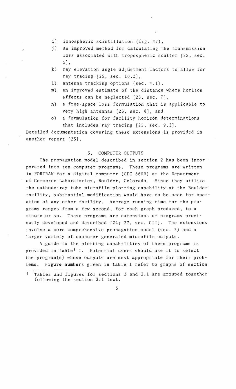
i) ionospheric scintillation ( g. 47),
j) an improved method for calculating the transmission
loss associated with tropospheric scatter [25, sec.
5 J ' k) ray elevation angle adjustment factors to allow for
ray tracing [25, sec. 10.2],
1) antenna tracking options (sec. 4.1), m) an improved estimate of the distance where horizon
effects can be neglected [25, sec. 7],
n) a free-space loss formulation that is applicable to
very high antennas [25, sec. 8], and o) a formulation for facility horizon determinations
that includes ray tracing [25, sec. 9.2]. Detailed documentation covering these extensions is provided in another report [25].
3. COMPUTER OUTPUTS The propagation model described in section 2 has been incor
porated into ten computer programs. These programs are written in FORTRAN for a digital computer (CDC 6600) at the Department of Commerce Laboratories, Boulder, Colorado. Since they utilize
the cathode-ray tube microfilm plotting capability at the Boulder
facility, substantial modification would have to be made for oper
ation at any other facility. Average running time for the pro
grams ranges from a few second, for each graph produced, to a minute or so. These programs are extensions of programs previ
ously developed and described [24; 27, sec. CII]. The extensions
involve a more comprehensive propagation model (sec. 2) and a
larger variety of computer generated microfilm outputs. A guide to the plotting capabilities of these programs is
provided in table3 1. Potential users should use it to select
the program(s) whose outputs are most appropriate for their problems. Figure numbers given in table 1 refer to graphs of section
3 Tables and figures for sections 3 and 3.1 are grouped together following the section 3.1 text.
5
3.1. Short discussions for each capability are given 1n section
3.2. Simple problem applications involving the graphs of section
3.1 are provided in section 3.3. Some additional graphs and prob
lems are given in Appendix A. Input parameters needed to operate
the various programs and plotting options such as a choice of
English or metric units (table 4) are discussed in section 4.
Each program causes the computer to produce (a) listings of
parameters associated with particular runs and (b) microfilm
plots. These outputs are provided for each parameter set used as
input to the computer and are tied to each other by a run code
consisting of the date and time at which calculations for a par
ticular parameter set started.
Parameter sheets for all programs have a similar format and
provide similar information. In programs associated with inter
renee analysis, a parameter sheet is produced for both the de
sired and undesired facility when the input parameters associated
with them are not identical [24, figs. 8, 9].
Computer produced parameter sheets do not have dual English/
metric units and are either English or metric depending on the
unit option selected (sec. 4.3). Sample parameter sheets similar,
except for dual units, to those produced by the programs are
shown in figures3 1 through 5. These parameters were used in de
veloping the curves provided in section 3.1 to illustrate the
plotting capabilities of the programs. Systems considered are
Air Tra c Control communications (ATC, fig. 1), Instrument
Landing System (ILS, fig. 2), UHF Satellite (fig. 3), Tactical
Air Navigation (TACAN, fig. 4), and VHF Omni directional Range
(VOR, fig, 5). Parameters are given in about the same order as
they are discussed in section 4.1. The effective area, AI, re
quired to convert power density, SR, to power available at the
output of an ideal (loss less) isotropic receiving antenna, PI,
is given at the bottom of the parameter sheets for power density
predictions (figs. 1, 2, 4, 5); i.e.,
6
3.1 GRAPHS
Figures 6 through 39 are sample graphs associated with the
various capabilities summarized in table 1. These graphs are
meant to illustrate general capability and care should be taken
in using them for particular problems where the parameters re
quired may differ from those used to develop the graphs. They
should be used, rather, as examples to help select the graph
types that are most appropriate for the particular applications.
Graphs produced by the computer are very similar to these, but
do not include all the labeling. In particular, the supplemen
tary scale is not computer generated and only provides an approx
imate correspondence with primary units. More accurate readings
can be obtained by using the primary scale, and then converting to
the desired units by using an appropriate conversion factor (p.ii).
This method was used to obtain dual values for readings given in
the text.
Options available (sec. 4.3) for units result in the plotting
of the primary grid and heading data in English (nautical or sta
tute) miles, or metric units. Except for figures 6 through 15
where the metric option was used, all figures in this section were
generated with the nautical mile option. An option to plot a
gainst central angle (fig. 41) instead of distance was used to
produce figure 16.
4 The notation used for the units of these quantities is intended to imply that they are decibel-type quantities obtained by taking 10 log of a quantity with the units indicated after dB-; e.g., A [dB-sq m] = 10 log {A 2 [sq m]/4n)} (where A [m] is wavelen~th). Equations used in this report are dimensionally consistent. Where difficulties with units could occur, brackets are used to indicate proper units.
7

Table 1. Plot!ing~ C~pabili ty Guide
Capability
Lobing**
Reflection coefficient**
rath length difference**
Time lag**
Lobing frcquency-D**
Lobing frequency-Hww
Reflection point**
Elevation angleR*
Flevation angle difference**
Spectral plotw*
Power available
!'ower density
Transmission loss
Power available curves
Power density curves
Transmission loss curves
Power available volume
Power density volume
Transmission loss volume
r:r RP contours
Power available contours
Power density contours
Transmission loss contours
Signal ratio-S
Figure(s)* Program
6 LOBING
7
8
9
10
11
12
13
14
lS
16
17-19
20
21
22
23
24
25
26
30
31
32
33
LOBING
LOBING
LOBING
LOBING
LOBING
LOBING
LOBING
LOBING
LOBING
ATOA
ATOA
ATOA
ATLAS
ATLAS
ATLAS
III POD
JIIPOD
HI POD
APODS
;\PODS
APODS
APODS
A TAll./
8
Remarks
Transmission loss versus path distance.
Effective specular reflection coefficient versus path distance.
Difference in reflected and direct ray lengths versus path distance.
Same as above with path length difference expressed as time delay.
Normalized distance lobing frequency versus path distance.
Normalized height lobing frequency versus path distance.
Distance to reflection point versus path distance,
Direct ray elevation angle versus path distance.
Angle by which the direct ray exceeds the reflected ray versus path distance.
~litude versus frequency response curves for various path distances.
Power available at receiving antenna versus path distance or central angle for time availabilities ·s, SO, and 9S percent.
Similar to above, but with power density ordinate.
Similar to above, but with transmission loss ordinate.
Power available curves versus distance are provided for several aircraft altitudes with a selected time availability, and a fixed lower antenna height.
Similar to above, but with power density as ordinate.
Similar to above, but with transmission loss as ordinate.
Fixed power available contours in the altitude versus distance plane for time availabilities of S, SO, and 9S percent.
Similar to above, but with fixed power density contours.
Similar to above, but with fixed transmission loss contours.
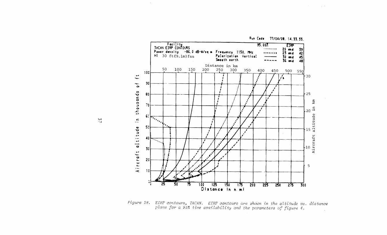
Contours for several EIRP levels needed to meet a particular power density requirement are shown in the altitude versus distance plane for a single time availability.
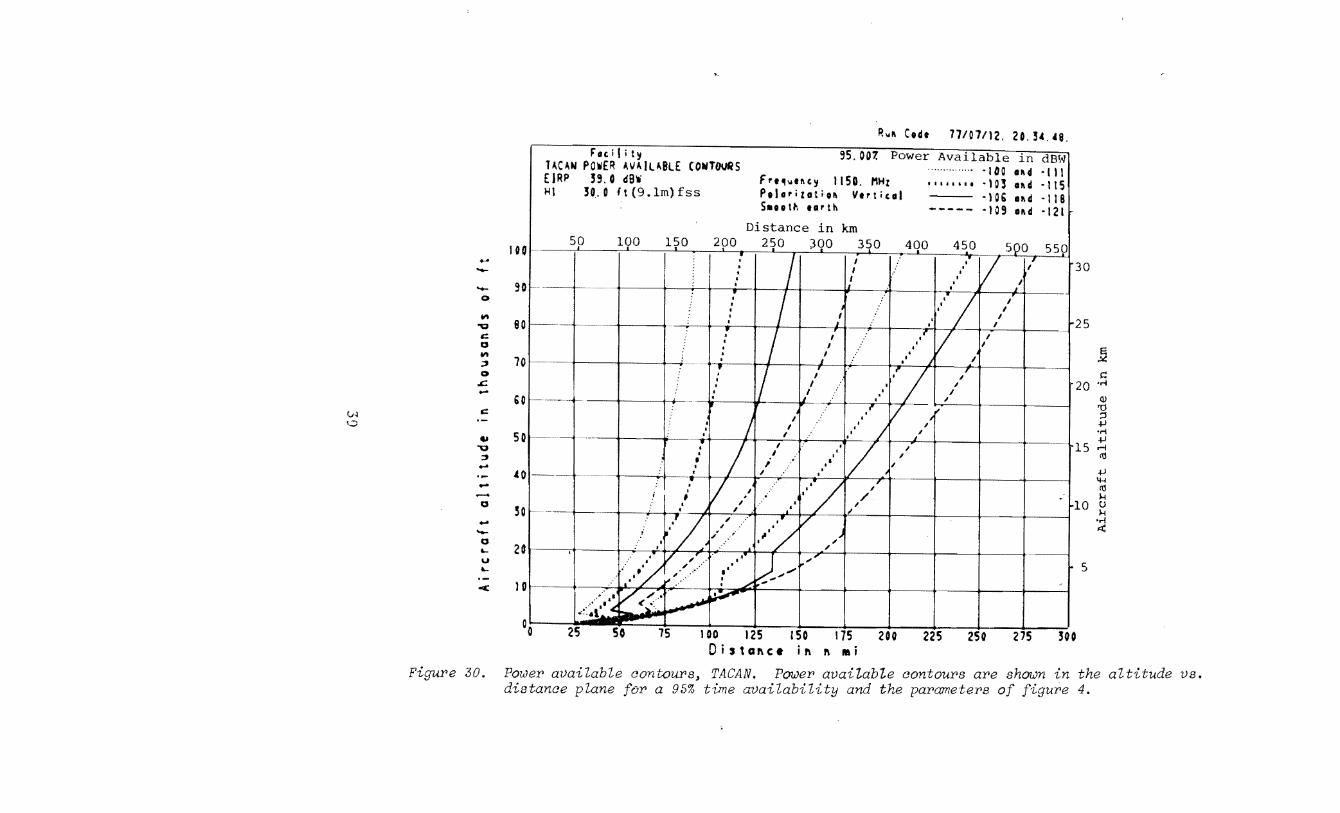
Similar to above, but with power available contours fOr a single EIRP.
Similar to above, but with power density contours.
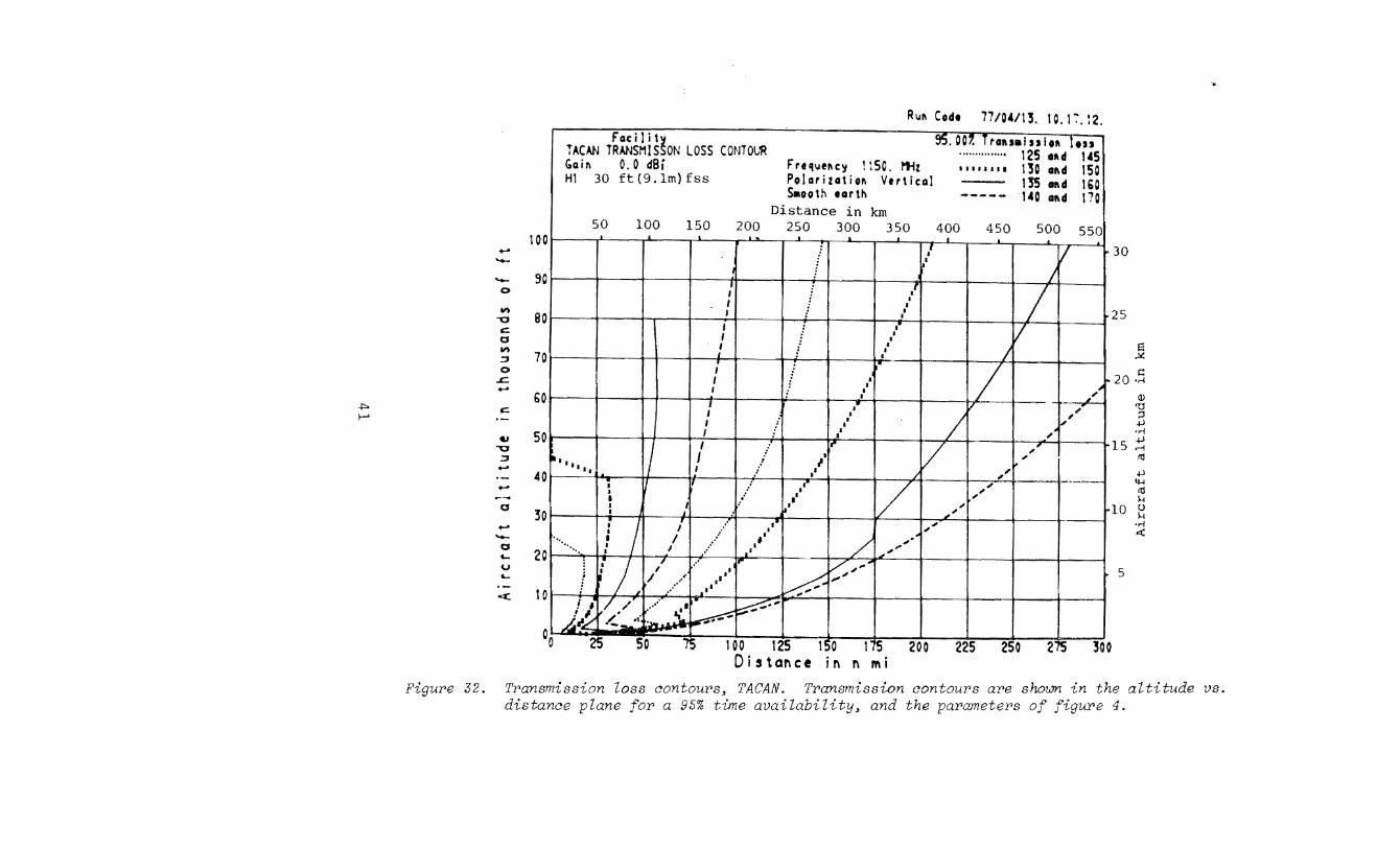
Similar to above, but with transmission loss contours.
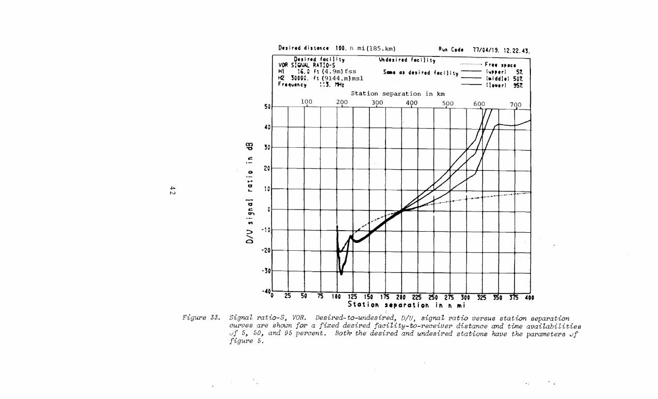
Desired-to-undesired, D/U, signal ratio versus station separation for a fixed desired facility-to-receiver distance, and time availabilities of S, SO, and 95 percent.

Capability
Signal ratio-DO
Orientation
Service volume
Signal ratio contours
_j~Jot t_irlg C<1:_pab il i ty Guide L<:_<.'_!l:!_-_1
Figure(s)* Program
34 OODD
35 TWIRL
36-37 SRVWM
38-39 DURATA
Similar to above, but abscissa is desired facility·to· receiver distance and the station separation is fixed.
Undesired station antenna orientation with respect to the desired to undesired station line versus required facility separation curves are plotted for several desired station antenna orientations. These curves show the maxinun separation required to obtain a specified D/U signal ratio value at several aircnft locations (i.e., protection points).
Fixed D/U contours are shown in the altitude venus distance plane for a fixed station separation and time availabilities of S, SO, and 95 percent.
Contours for several D/U values are shown in the altitude versus distance plane for a fixed station separation and time availability.
Additional discussion, by capability, is provided in the text. *~ Applicable only to the line·of·sight region for spherical earth geanetry. Variability with time and
horizon effects are neglected and the counterpoise option is not available. The phase change associated with surface reflection in the lobing region is taken as 0 or 180° to avoid missing lobe nulls.
9
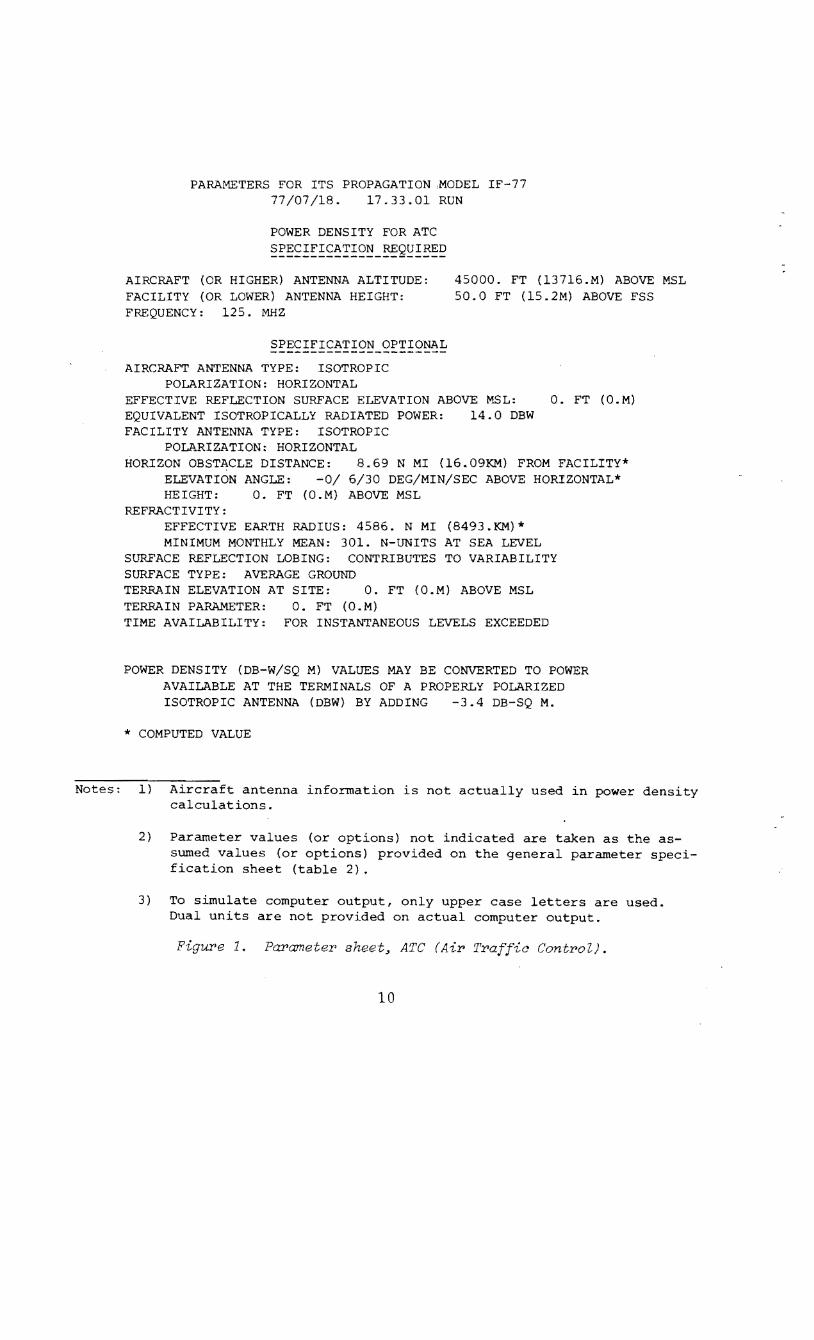
PARAMETERS FOR ITS PROPAGATION ,MODEL IF-77 77/07/18. 17.33.01 RUN
POWER DENSITY FOR ATC
~~~~!~!~~!!9~-~9~!~~
AIRCRAFT (OR HIGHER) ANTENNA ALTITUDE: FACILITY (OR LOWER) ANTENNA HEIGHT: FREQUENCY: 125. MHZ
SPECIFICATION OPTIONAL
AIRCRAFT ANTENNA TYPE: ISOTROPIC POLARIZATION: HORIZONTAL
45000. FT (13716.M) ABOVE MSL 50.0 FT (15.2M) ABOVE FSS
EFFECTIVE REFLECTION SURFACE ELEVATION ABOVE MSL: 0. FT (O.M) EQUIVALENT ISOTROPICALLY RADIATED POWER: 14.0 DBW FACILITY ANTENNA TYPE: ISOTROPIC
POLARIZATION: HORIZONTAL HORIZON OBSTACLE DISTANCE: 8.69 N MI (16.09KM) FROM FACILITY*
ELEVATION ANGLE: -0/ 6/30 DEG/MIN/SEC ABOVE HORIZONTAL* HEIGHT: 0. FT (O.M) ABOVE MSL
REFRACTIVITY: EFFECTIVE EARTH RADIUS: 4586. N MI (8493.KM)* MINIMUM MONTHLY MEAN: 301. N-UNITS AT SEA LEVEL
SURFACE REFLECTION LOBING: CONTRIBUTES TO VARIABILITY SURFACE TYPE: AVERAGE GROUND TERRAIN ELEVATION AT SITE: 0. FT (O.M) ABOVE MSL TERRAIN PARAMETER: 0. FT (O.M) TIME AVAILABILITY: FOR INSTANTANEOUS LEVELS EXCEEDED
POWER DENSITY (DB-W/SQ M) VALUES MAY BE CONVERTED TO POWER AVAILABLE AT THE TERMINALS OF A PROPERLY POLARIZED ISOTROPIC ANTENNA (DBW) BY ADDING -3.4 DB-SQ M.
* COMPUTED VALUE
Notes: 1) Aircraft antenna information is not actually used in power density calculations.
2) Parameter values (or options) not indicated are taken as the assumed values (or options) provided on the general parameter specification sheet (table 2).
3) To simulate computer output, only upper case letters are used. Dual units are not provided on actual computer output.
Figure 1. Parameter sheet~ ATC (Air Traffic Control).
10

PARAMETERS FOR ITS PROPAGATION MODEL IF-77 77/07/19. 11.39.28. RUN
POWER DENSITY FOR ILS
~~~~!~!~~!!2~-~9~!~~ AIRCRAFT (OR HIGHER) ANTENNA ALTITUDE: FACILITY (OR LOWER) ANTENNA HEIGHT: FREQUENCY: 110. MHZ
SPECIFICATION OPTIONAL
AIRCRAFT ANTENNA TYPE: ISOTROPIC POLARIZATION: HORIZONTAL
6250. FT (1905.M) ABOVE MSL 5.5 FT (1.68M) ABOVE FSS
EFFECTIVE REFLECTION SURFACE ELEVATION ABOVE MSL: 0. FT (O.M) EQUIVALENT ISOTROPICALLY RADIATED POWER: 24.0 DBW FACILITY ANTENNA TYPE: 8-LOOP ARRAY (COSINE VERTICAL PATTERN)
POLARIZATION: HORIZONTAL HORIZON OBSTACLE DISTANCE; 2.88 N MI (5.33KM) FROM FACILITY*
ELEVATION ANGLE: · -0/ 2/09 DEG/MIN/SEC ABOVE HORIZONTAL* HEIGHT: 0. FT ABOVE MSL
REFRACTIVITY: EFFECTIVE EARTH RADIUS: 4586. N MI (8493.KM)* MINIMUM MONTHLY MEAN: 301. N-UNITS AT SEA LEVEL
SURFACE REFLECTION LOBING: CONTRIBUTES TO VARIABILITY SURFACE TYPE: AVERAGE GROUND TERRAIN ELEVATION AT SITE: 0. FT (O.M) ABOVE MSL TERRAIN PARAMETER: 0. FT (O.M) TIME AVAILABILITY: FOR INSTANTANEOUS LEVELS EXCEEDED
POWER DENSITY (DB-W/SQ M) VALUES MAY BE CONVERTED TO POWER AVAILABLE AT THE TERMINALS OF A PROPERLY POLARIZED ISOTROPIC ANTENNA (DBW) BY ADDING -2.3 DB-SQ M.
* COMPUTED VALUE
Notes: 1) Aircraft antenna information is not actually used in power density calculations.
2) Parameter values (or options) not indicated are taken as the assumed values (or options) provided in the general parameter specification sheet (table 2).
3) To simulate computer output, only upper case letters are used. Dual units are not provided on actual computer output.
Figure 2. Parameter sheet~ ILS (Instrument Landing System)
11
Notes:
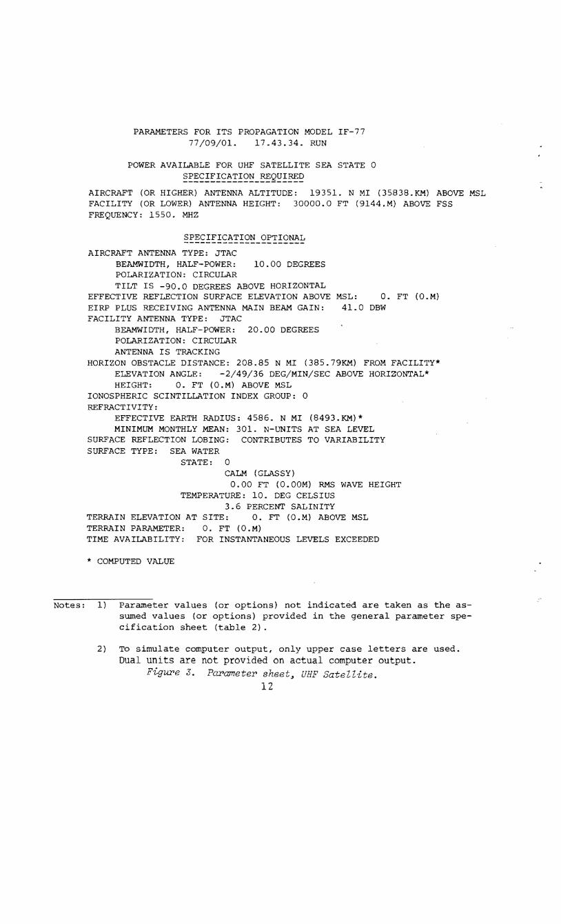
PARAMETERS FOR ITS PROPAGATION MODEL IF-77 77/09/01. 17.43.34. RUN
POWER AVAILABLE FOR UHF SATELLITE SEA STATE 0
~~~~~~~~~!~2~-~9~!~~ AIRCRAFT (OR HIGHER) ANTENNA ALTITUDE: 19351. N MI (35838.KM) ABOVE MSL FACILITY (OR LOWER) ANTENNA HEIGHT: 30000.0 FT (9144.M) ABOVE FSS FREQUENCY: 1550. MHZ
SPECIFICATION OPTIONAL
AIRCRAFT ANTENNA TYPE: JTAC BEAMWIDTH, HALF-POWER: 10.00 DEGREES POLARIZATION: CIRCULAR TILT IS -90.0 DEGREES ABOVE HORIZONTAL
EFFECTIVE REFLECTION SURFACE ELEVATION ABOVE MSL: 0. FT (O.M) EIRP PLUS RECEIVING ANTENNA MAIN BEAM GAIN: 41.0 DBW FACILITY ANTENNA TYPE: JTAC
BEAMWIDTH, HALF-POWER: 20.00 DEGREES POLARIZATION: CIRCULAR ANTENNA IS TRACKING
HORIZON OBSTACLE DISTANCE: 208.85 N MI (385.79KM) FROM FACILITY* ELEVATION ANGLE: -2/49/36 DEG/MIN/SEC ABOVE HORIZONTAL* HEIGHT: 0. FT (O.M) ABOVE MSL
IONOSPHERIC SCINTILLATION INDEX GROUP: 0 REFRACTIVITY:
EFFECTIVE EARTH RADIUS: 4586. N MI (8493.KM)* MINIMUM MONTHLY MEAN: 301. N-UNITS AT SEA LEVEL
SURFACE REFLECTION LOBING: CONTRIBUTES TO VARIABILITY SURFACE TYPE: SEA WATER
STATE: 0 CALM (GLASSY)
0.00 FT (O.OOM) RMS WAVE HEIGHT TEMPERATURE: 10. DEG CELSIUS
3.6 PERCENT SALINITY TERRAIN ELEVATION AT SITE: 0. FT (O.M) ABOVE MSL TERRAIN PARAMETER: 0. FT (O.M) TIME AVAILABILITY: FOR INSTANTANEOUS LEVELS EXCEEDED
* COMPUTED VALUE
Parameter values (or options) not indicated are taken as the assumed values (or options) provided in the general parameter specification sheet (table 2) .
2) To simulate computer output, only upper case letters are used. Dual units are not provided on actual computer output.
Figure 3. Parameter sheet~ UHF Satellite. 12

PARAMETERS FOR ITS PROPAGATION MODEL IF-77 77/07/19. 11.39.31. RUN
POWER DENSITY FOR TACAN SPECIFICATION
AIRCRAFT (OR ANTENNA ALTITUDE: 40000. FT (12192.M) ABOVE MSL FACILITY (OR LOWER) ANTENNA HEIGHT: 30.0 FT (9.14M) ABOVE FSS FREQUENCY: 1150. MHZ
SPECIFICATION OPTIONAL
AIRCRAFT ANTENNA TYPE: ISOTROPIC POLARIZATION: VERTICAL
EFFECTIVE REFLECTION SURFACE ELEVATION ABOVE ~$L: EQUIVALENT ISOTROPICALLY RADIATED POWER: 39.0 DBW FACILITY ANTENNA TYPE: TACAN (RTA-2)
POLARIZATION: VERTICAL
0. FT (O.M)
HORIZON OBSTACLE DISTANCE 6.73 N MI (12.46KM) FROM FACILITY* ELEVATION ANGLE: -0/ 5/ 2 DEG/MIN/SEC ABOVE HORIZONTAL* HEIGHT: 0. FT (O.M) ABOVE MSL
REFRACTIVITY: EFFECTIVE EARTH RADIUS: 4586. N MI (8493.KM)* MINIMUM MONTHLY MEAN: 301. N-UNITS AT SEA LEVEL
SURFACE REFLECTION ~OBING: CONTRIBUTES TO VARIABILITY SURFACE TYPE: AVERAGE GROUND TERRAIN ELEVATION AT SITE: 0. FT (O.M) ABOVE MSL TERRAIN PARAMETER: 0. FT TIME AVAILABILITY: FOR INSTANTANEOUS LEVELS EXCEEDED
POWER DENSITY (DB-W/SQ M) VALUES MAY BE CONVERTED TO POWER AVAILABLE AT THE TERMINALS OF A PROPERLY POLARIZED ISOTROPIC ANTENNA (DBW) BY ADDING -22.7 DB-SQ M.
* COMPUTED VALUE
Notes: 1) Aircraft antenna information is not actually used in power density calculations.
2) Parameter values (or options) not indicated are taken as the assumed values (or options) provided in the general parameter specification sheet (table 2).
3) To simulate computer output, only upper case letters are used. Dual units are not provided on actual computer output.
Figu:tae 4. Pa1.1ameteP sheet~ TACAN (Tactical AiP Navigation}.
13
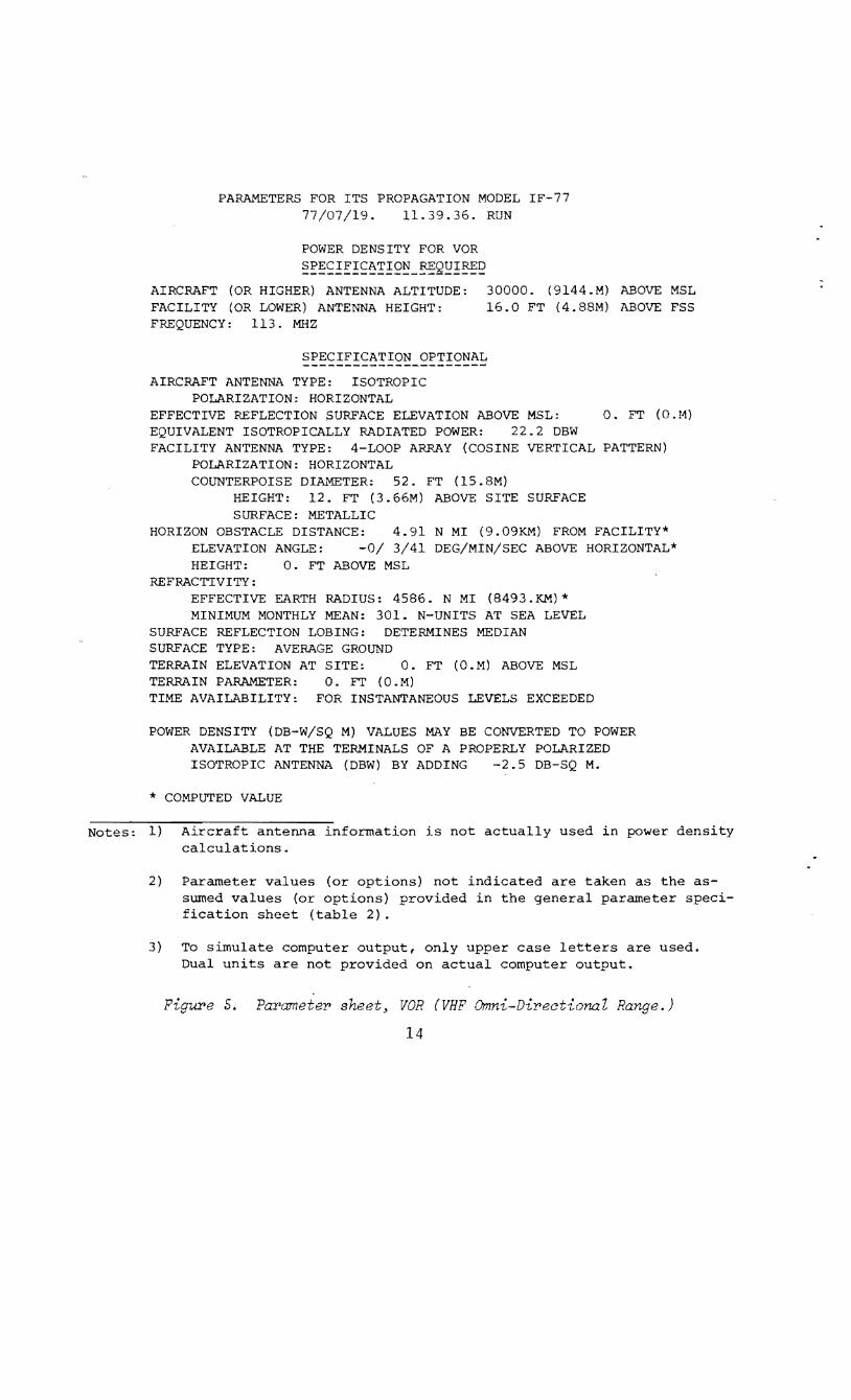
PARAMETERS FOR ITS PROPAGATION MODEL IF-77 77/07/19. 11.39.36. RUN
POWER DENSITY FOR VOR
~~~~~~~~~~~Q~-~Q~~~Q AIRCRAFT (OR HIGHER) ANTENNA ALTITUDE: FACILITY (OR LOWER) ANTENNA HEIGHT:
30000. (9144.M) ABOVE MSL 16.0 FT (4.88M) ABOVE FSS
FREQUENCY: 113. MHZ
SPECIFICATION OPTIONAL
AIRCRAFT ANTENNA TYPE: ISOTROPIC POLARIZATION: HORIZONTAL
EFFECTIVE REFLECTION SURFACE ELEVATION ABOVE MSL: EQUIVALENT ISOTROPICALLY RADIATED POWER: 22.2 DBW
0. FT (0. !-1)
FACILITY ANTENNA TYPE: 4-LOOP ARRAY (COSINE VERTICAL PATTERN) POLARIZATION: HORIZONTAL COUNTERPOISE DIAMETER: 52. FT (15.8M)
HEIGHT: 12. FT (3.66M) ABOVE SITE SURFACE SURFACE: METALLIC
HORIZON OBSTACLE DISTANCE: 4.91 N MI (9.09KM) FROM FACILITY* ELEVATION ANGLE: -0/ 3/41 DEG/MIN/SEC ABOVE HORIZONTAL* HEIGHT: 0. FT ABOVE MSL
REFRACT'IVITY: EFFECTIVE EARTH RADIUS: 4586. N MI (8493.KM)* MINIMUM MONTHLY MEAN: 301. N-UNITS AT SEA LEVEL
SURFACE REFLECTION LOBING: DETERMINES MEDIAN SURFACE TYPE: AVERAGE GROUND TERRAIN ELEVATION AT SITE: 0. FT (O.M) ABOVE MSL TERRAIN PARAMETER: 0. FT (O.M) TIME AVAILABILITY: FOR INSTANTANEOUS LEVELS EXCEEDED
POWER DENSITY (DB-W/SQ M) VALUES MAY BE CONVERTED TO POWER AVAILABLE AT THE TERMINALS OF A PROPERLY POLARIZED ISOTROPIC ANTENNA (DBW) BY ADDING -2.5 DB-SQ M.
* COMPUTED VALUE
Notes: 1) Aircraft antenna information is not actually used in power density calculations.
2) Parameter values (or options) not indicated are taken as the assumed values (or options) provided in the general parameter specification sheet (table 2).
3) To simulate computer output, only upper case letters are used. Dual units are not provided on actual computer output.
Figure 5. Parameter sheet~ VOR (VHF Omni-Directional Range.)
14

~ .... V1
R~JII Ctdt 71/0711'. 17 . .tB. 57.
,-----rRANSMISSION LOSS ·-HI tS. • (SO.Oft)rnsl Smooth earth H2 t371&. • (45000. f.t)rnsl Polarization Horizontal rrtjjuUCy 12S. f1Hz
Distance in n rni
91) 0 40 60 80 120 110 140 160 180 220 220 240 ---· ------· I ' I I I -L---
90
m "U
I 0 0 c -.... 110 .... 0 -c 120 0 -.... .... no -li .... c::
I .CO 0 ._ 1-
~~ Lobe 4 --·~~ -
... Lobe 3 (\ •- . Lobe 2 . ··- ·-~oo,_
---~ ·-~ .. (. ·~ ····· ... ········ Lobe l In phase ··•·· ... ········ .. I I 1 lf 1 ---~
(low loss) I 0 I ........ .......... .
~ II I I I I • I I·!· I I t -.....
... ········ I-- --·-·. -. Free sp • • • • • ,,, 1'----
~ • I I
~ j ace loss ... • . '- ..
\ I "r-f-- •. -·--r-·-
·l·-. .\ . ..
ISO
1~0
t7
... 1--- .. -
· .. ·· -... .. Out of phase _.-· · · · ... ...... (high loss) J...-·
r-- -- ···--.. ... _tee ----············· ~~-
0 2S so 75 I 00 125 ISO l15 200 225 2SO 275 300 325 350 3'J5 400 425 450 H~ Oistal\ce il\ kll\
Figur>e 6. Lobing, ATC. Tr>ansm1:ssion loss for> the fir>st ten lobes inside the r>adi._; hor>izon, limi values associated ZJith in and out of phase conditions and fr>ee-space Z.oss vs. oath distance ar>e shOZJn. These cur>ves 1Jer'e computed for> the pcwconetePs of fiJUY'e 1.

0::: ... u ·---... 0 u
0: 0
r-a 0\ u ... --... ....
... > --u ... --w
R ... ~ Code 77107/ll. 17.,8. 37
REFLECTION COEFFICIENT HI 15. 111 (50. Oft)msl · Smooth earth H2 1371 G. 111 (45000. ft)msl Polarization Horizontal frequHcy 125. MHt
Distance in n mi
1. 210 40 60 80 1po 1(0 1~0 160 1~0 2QO 220 240 I
I 1.6
~ ~ ...
,/ v
'; .B
6
.4
.z
0' o, zs so 75 too 125 1so 175 200 225 25a 275 no 325 350 375 4oo 425 450 .ns
Oistal'\ce il'\ k"'
Figure 7. Reflection coefficient, ATC. Effective reflection coefficient vs. path distance is shOI.Jn for the parcuneters of figure 1.
A1111 'odt 71/07/IA. t1. 48. 31.
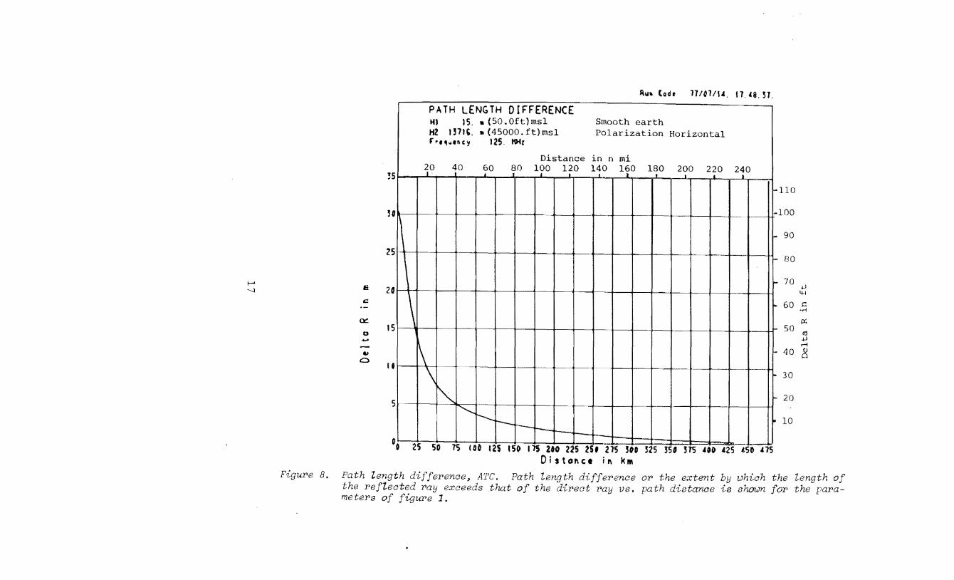
PATH LENGTH DIFFERENCE --HI 15. • (50.0ft)msl Smooth earth H2 1371G. • (45000. ft)msl Polarization Horizontal r •• ~ .. tllcy 125. HHt
Distance in n mi
35 ~0 40 60 80 100 120 140 1~0 180 200 220 240 • I • •
1- 110
1·-f- -
1\ r--
i-
100
90
30
25 t- 80
f-' e 20 ---.)
c. ·-~
15 0
~
\ 70 .jJ
4-4
60 c •rl
p:; 50
C!l ... .jJ
-.. 0 .. 1\ 1-
\ ··~ --
r-i
40 ~
30
"" 1'-
["-.... r--r- '" r--t--
20
10
5
L.._ __ -00 25 50 71) 10~ 125 ISO 11S 200 225 2St 275 500 325 351 315 AOO 425 tSO HS
Dis tone• i 1'\ k111
Figure B. Path 'length difference, ATC. Path length difference or the extent by uJhich the length of the reflected ray that of the direct ray vs. path distance is shown for para-meters of figure 1.
...... co
u ... .... .:0:
0:::
0'\ a
... 6 -t-
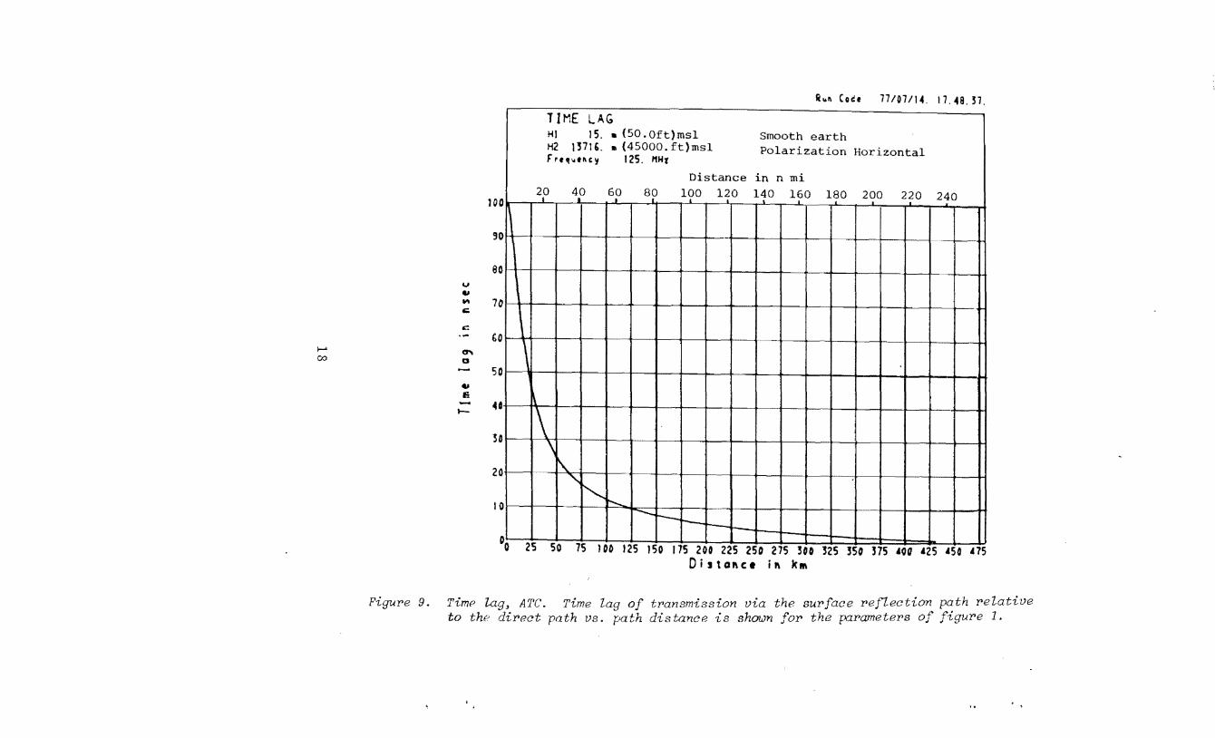
lh11 Cotle 71/07114. 17. 48. n TIME LAG HI 15. • (SO.Oft)msl Smooth earth H2 1371G. • (45000. ft)msl Polarization Horizontal Fre.,.ency 125. t114t
Distance in n mi
100
30
2p 40 6? 80 100 120 140 160 180 200 220 240 ' .
~~· ao
10
!;O
50
\
\ 41
30 1\ \
20 t- i\.
" I 0
~ 1"--.... ....._
t---I--0o 25 so 75 1 oo 125 J5o 175 2oo 225 250 275 300 325 3So ns •oo •2s •so ns
Distol\ct il\ k111
FiguPe 9. Time tag, ATC. Time lag of tPansmission via the suPface peflection path Pelative to the direct path vs. path distance is shown for the parameters of figuPe 1.

~ .. 11 Codt 11/071\4. 11. 48. 31.
NORMALIZED DISTANCE LOSING FREQUENCY I-ll 15. • (SO.Oft)msl Smooth Earth H2 1371&. • (45000.ft)msl Polarization Horizontal f r tllwtll cy 125. 11Hz
Distance in n mi
IL..
20 40 60 80 1po 120 140 lpO 180 200 2f0 ~40 I 1.0 .c 1.8 ......... e
""' I .~
(j) -......... - I .a .8 1. 6 .t!
' -.... X - N
1.4 :r: 8
......... .... :r: -
' .1 ' N :r:
1.2 ,;: ' .6 c
·.-l .......
~
\D
c: ·-.Q 0 -
;
4
.5
4
l.O tl' c ·.-l .a 0
0.8 r-1
<lJ u ..,
u c: 0 -.... ·-0
5 l\
1\ ?
\
c 0.6 m
.1-l (j)
·.-l Cl
0.4
I
" I'-r--. I 0
o. ·o 2s so 75 100 125 cso 175 200 225 250 21s 3oo 325 350 375 .eu 425 .eso .t1S
0.2
Oista~ce ift ka ·
10. ATC. vs. pa

N 0
R-.11 ~ode 71107114. 11. 48. H.
NORMALIZED HEIGHT LOSING FREQUENCY HI 15. • (50. Oft)ms1 Smooth·earth H2 1511G. • (45000. ft)ms1 Polarization Horizontal ~ •t~1.1fH!; 125. 11H%
Distance in n mi
. Ot 20 40 60 80 100 1~0 1~0 160 180 200 220 240
0 L -~ .018 -e.
....... s ~
c •.-t
. DS
F. ~
....... ......
~ . " "
.016 1':
' +J '~--<
. DS
-·~ I 1-....... .....
:r;: ~
~ ·-
" " 1\ D
\ )
\
.014 ' ..-N :r:
. 012 E-t
' N :r:
.010 c
.04
.04
03
en ~
·-A 0
D
1\ 5 \
•.-t
0"
.008 -~ ..a 0
r-l
03
. 02
-..If: 0
' . 01 4J
:X: .01
0
"' ) " ' ~ 0 b-.
.006 ~ o·
·.-t ())
. 004 :r:
. Ol
...__ --r--- 1-s .002 QO
0.00 00 2S 50 . 75 I 00 125 ISO 175 2ot 225 250 2 5 !00 325 350 H5 400 425 A 50 A75 Distance in k•
Figure 11. Lobing frequency-H, ATC. Normalized height lobing frequency, NHLF, vs. path distance is shown for the parameters of figure 1.
. .

t'<,)
f--1
'\.
e ~
.:: --.:: -0 Q..
c 0 -.. u
"' --"' .... 0 -"' u c a -"" ·-
0
Ru~ Code 17/07/14. 17. 48. H.
REFLECTION POINT DISTANCE HI 15. • (50. Oft)msl Smooth earth H2 IHIG. • (45000.ft)msl Polarization Horizontal f't1Uf11Cy 125. ttH:
Distance in n mi 20 40 60 80 100 120 140 160 180 200 220 240
I . 1/ I
2.0
I. 8
~,, I ~ '
I ' ' v l . "
I I. 2
I 1.0 / B .8 I
/
.b b v v v "
/ v
,....,.-' .,..-
i---~ i------_,..,..-.-
'\ -I- ..__ __
o. ·o 25 so 75 100 125 ISO 175 200 2Z5 250 215 nt 325 550 375 .tot .t25 .t5o .n5 Oistor.ce ir. k111
~
1.0
0.9
0.8
0.7
0.6
0.5
0.4
0.3
0.2
0.1
FiguPe 12. Reflection point, ATC. Distance fPom facility to tion point vs. ;Jath distance shown foP the paPametePs o.f figuPe 1.
.,
·r1 s s;::
s;:: ·r1
.jJ s;::
•r1 0 0.. s;:: 0
·r1 .jJ u Q)
.--l 4-1
<J)
k
0 .jJ
Q) u s;:: 11.1 .jJ (f)
·r1 0
N N
I lO
I 9 0"\ u
"0 8 l 0:: -
1 7 u -17'\ t: 0 ' c 0 5 5 ·-... 0 ::0. I. I. u -
L.a.J 1
I
I
RIJ~ Codt 17101111.. 17. 48. 37.
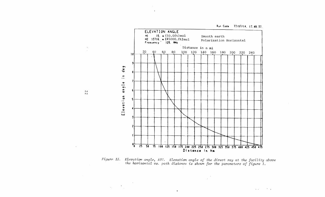
ELEVATION ANGLE HI 15. • (SO.Oft)rnsl Smooth earth H2 l37lG. • (45000. ft)rnsl Polarization Horizontal rrt4!Yfllq 125. 11Ht
Distance in n rni 20 40 60 80 100 120 140 160 180 200 220 240
. I
1\
1\ \ 1\
\ [\
\ ~
'\
1""-
""' ""' """ "' f'-..,. r---.. r---r-. r-- i--. 0 25 50 75 lDO 125 151 175 201 225 Z5Q 215 500 325 350 375 400 125 450 175
Oistaftce ift ka
Pigur>P 13. ElPVation angle, ATC. Elevation angle of the dir>ect my at the facility above the hor>izontal vs. path distance is shouJn for> the par>ameter>s of figur>e 1.
N VI
Rwt. Codt 17/011J4. 17. 48. 37.
ELEVATION ANGLE DIFFERENCE HI 15. • (SO.Oft)msl Smooth earth
0"\ ., "'C
H2 1371&. • (45000.ftlmsl Polarization Horizontal F'tt~uucy 125. ,.,..,
c Distance in n mi -., ~0 40 60 80 1po 120 140 l?O 180 200 220 240
I l 20 ::1"\ 0 ...
"'C ., -u ., --., ....
"'0 c 0
I 1\
\ \
--U I
r\ ' :I \ i l
1 B
1&
14
12
-u ., ... ·-"'0
I l\ I
\ I
I
""' I
'\
11
8
c: ., ., • -., "' .J ' ~ II
"' I ...Q
., -Ch c <
----.......
""" ~ ' t-.. r--r--r-- ~
I
0 25 SO 75 100 125 ISO 175 ZOO 22S 250 275 !OO !25 350 375 410 425 450 475 ·Oistal'lct il'l k"'
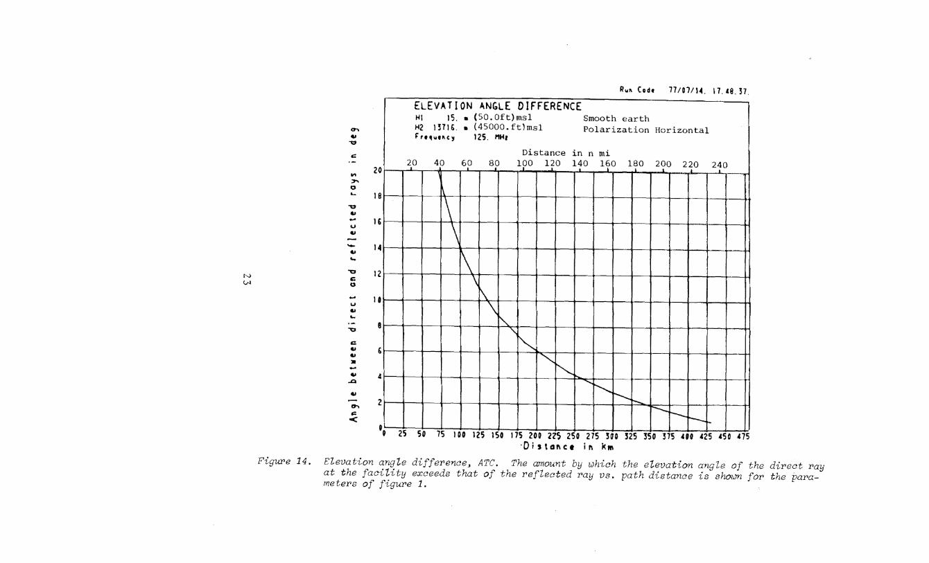
Figure 14. Elevation angle differenceJ ATC. The amount by which elevation angle of the direct ray at the facility exceeds that of the reflected ray vs. path distance is shmJn for the parameters of figure 1.
N +:..
T
SPECTRAL PLOT
8o11dw idth 100 kHz Lob• 1 t~ •
43 dB
Distance
1 v V 1kLobe 4 .. Frequency f-f f
f f f+fff
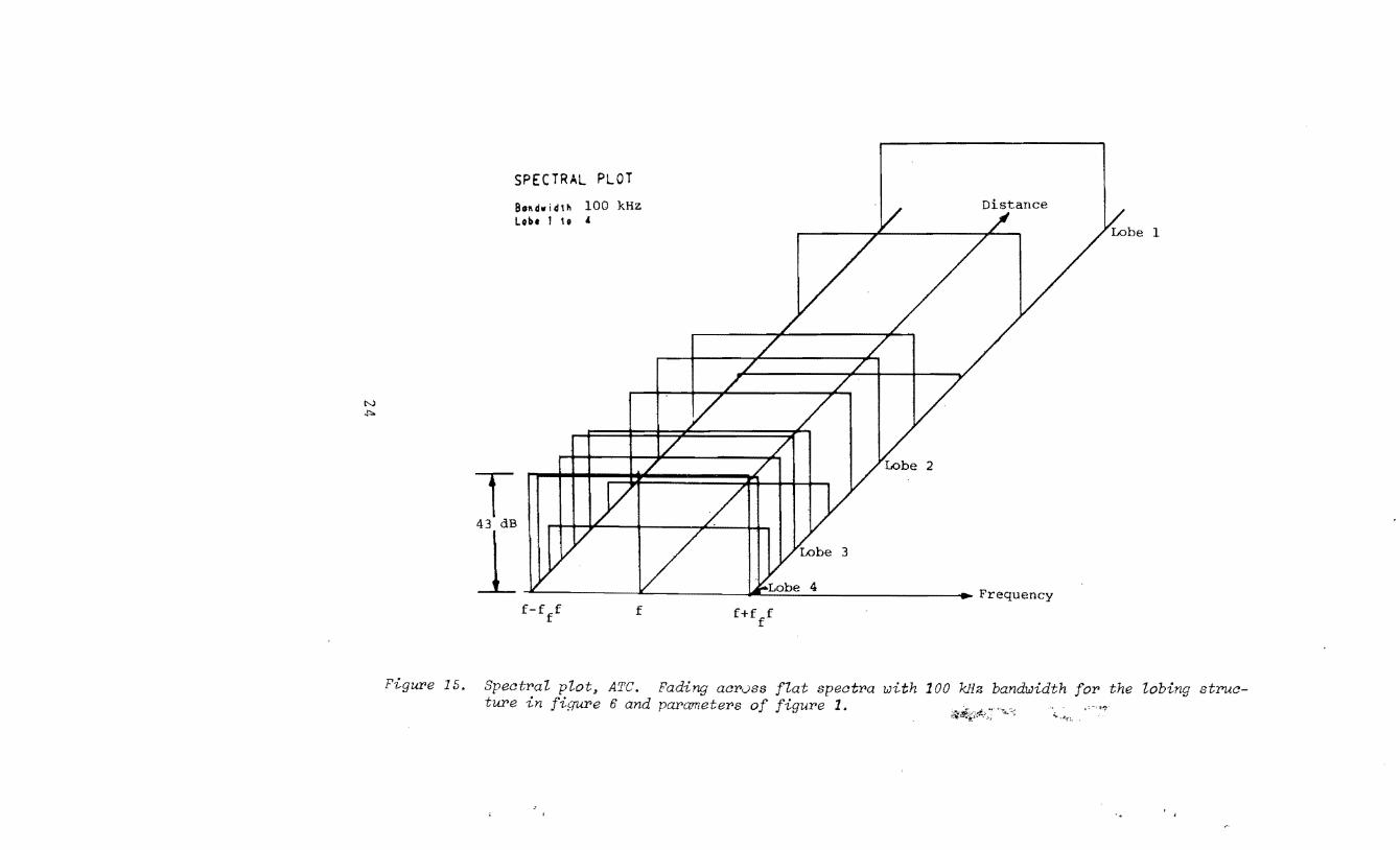
Figure 15. Spectral plot, ATC. Fading acrvss flat spectra with 100 kHz bandwidth for the lobing struc-ture in figure 6 and parameters of figure 1. ,.,..:.:- ........ ,_.... . ,-,~
"'~--~:
N t.n
=m "Q
·140
·ISO I
c: -lbO J
.... .n a ·17
a ::..
a ·18 ..... .... • 0
Q.. -19
-2 0
II
I
I
I
R~o~~ Collt 77/09/01. 17.43.34.
VHf SATELLITE SEA STATE C ... ·········· F' ttt SPOU F'rt~~o~tuy 1550. MHr EIRP' 41. 0 dBW ! ul''t rl s~ Hl 30000. ft{9l44.m} fss Saeotl\ tortl\ laictllltl so~ H2 1"51. ~ ai(35838.km)mslPtlaritotio~ Ci rc~o~lar !I o•trl 95~
·~--
--- ......
~ ~ ---·
"' ··- -
··-
' "
21 ·o 10 20 30 40 50 GO 70 80 90 Central angle in deg
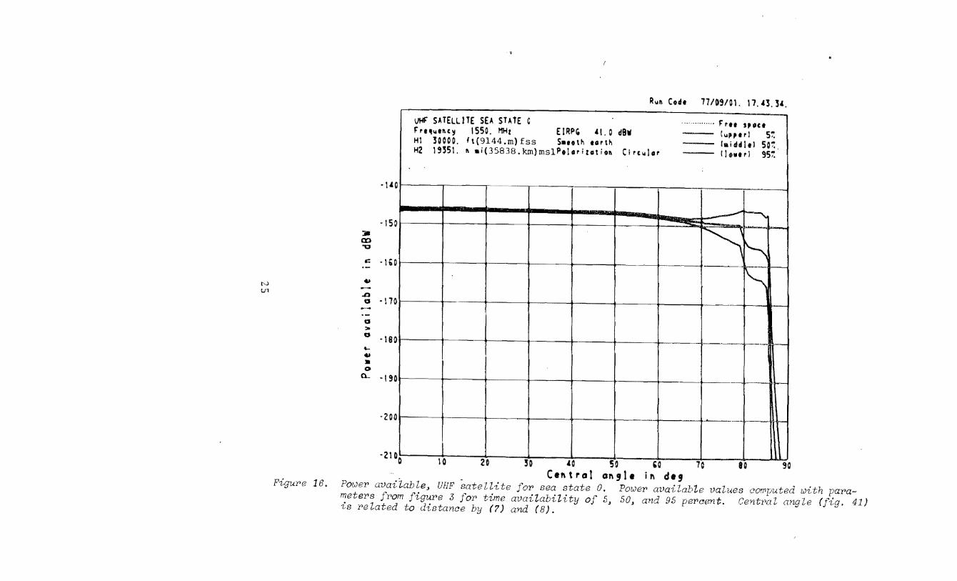
Figure 16. Power available~ UHF satellite for sea state Power available values computed w~th par'a-meters from figure 3 for time availability of 5, 50~ and 95 per!:!ent. Cent·ml ang (fig. 41) is related to distance by (7) and (8).

N Q'\
F'1~; 1Ul'(' 1 ,, ( .
R~a Ctdt 77/07/t!. lt. S!.21 .
lLS LOCALIZER ............... Frtt .,.,, Frt4jYtllCY 110. rt+a ElltP z•.o 4&w c-.,.,, 51. HI 5.5 ft(l.6Bm)fss Sattt" urt" la144ltl 501. H2 •zso. ft (190S.·.n}ms1 Pel.,iutita Her i Ita ttl lltwtrl t$1.
Distance in km
20 40 6,0 a,o 1~0 120 140 160 180 I L ·SO
a r:r IIIII
....... Jill
,t\ ,~'\
-u
·70 1
m -a ......
······ ·80 -= ,-~ ........ ~ ..........
-:n -·- '
··~ ................. ...................... I . . ................ ~. .. .............
~ -~~ ..... ,. ...... ~
-!0
IIIII
-= • 'U
~
• • 0 Q...
·11
J
~ ~ t--..... ~ ~ r---. r--:----..
' """' -...
~ ~ I --
·lGD
·110
·120
·t• I
' . - -. -- --·IS .. AI ID 20 lO •• ,, 101 •• so ,. 70 Ohtoftce 1ft ft aJ
Power density, ILS. Parameters used in the aaZculations are summarized in figure 2. This 9raph pr>ed1:cts power density on the ILS ZocaHzer front course. In other dir>ecHons, the pre<Hetions shouZd be adJusted according to the ZocaUzer> 's hori-zontaZ antenna patter>n.
..
Rva Code 77/07/19. II. 39.31.
TACAN 39.D 4Bw
···········-·· r ru ,,.u F'rt1utacy 1150. tttz ElRP lupperl 51. HI 30. It (9.lm}fss Sauth urth lalddltl 501. H2 •oooo. It (12192. m} msl Ptltriutlta Vert iul ···- llntrl !51.
Distance in km 50 100 l~O 2~0 2~0 3QO 3~0 400 450 sqo 550 I .,0
ll
&r
"' ....... ::.
I (X)
"'0
c -N
:n ~~ -
"' c
~ 1 oo
I!\ ,---- ._ 1,_ ..... -II- -
~ ~ ...... -....... ~ r--... ----~ ~ ~-- ........... -~-) .....
~ --.........
"' ~ ~ -1\\ ~ \
-70
·80
·90
-110 • "'0
.... • a 0
a..
\ ~" 0 ""' ~\ "" 0 -
·12
·13
\~ 0 ~
\ w--- . ------
·I•
·15
"" 10 25 so 75 I 00 125 I I D I '5 200 225 ~D 2 s so ·I' 0
Olttol\ce '" " al
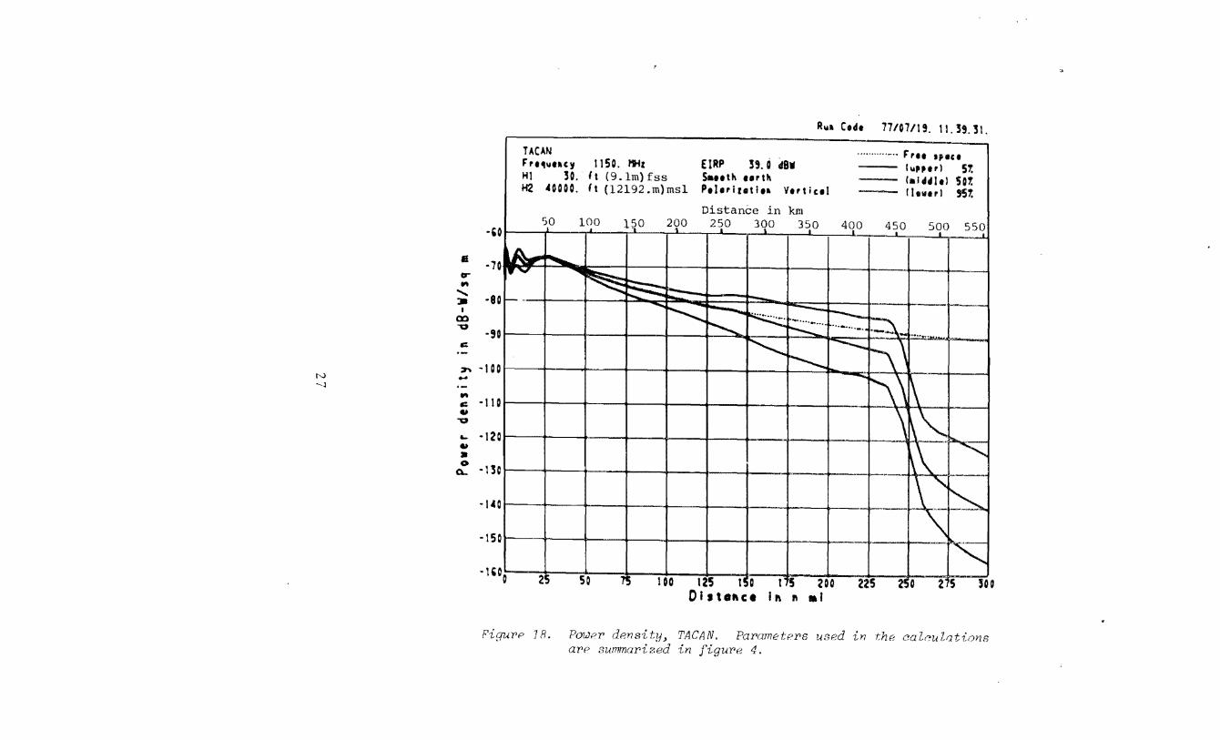
1 R. TACAN. Parametn•s used the ca are 4.
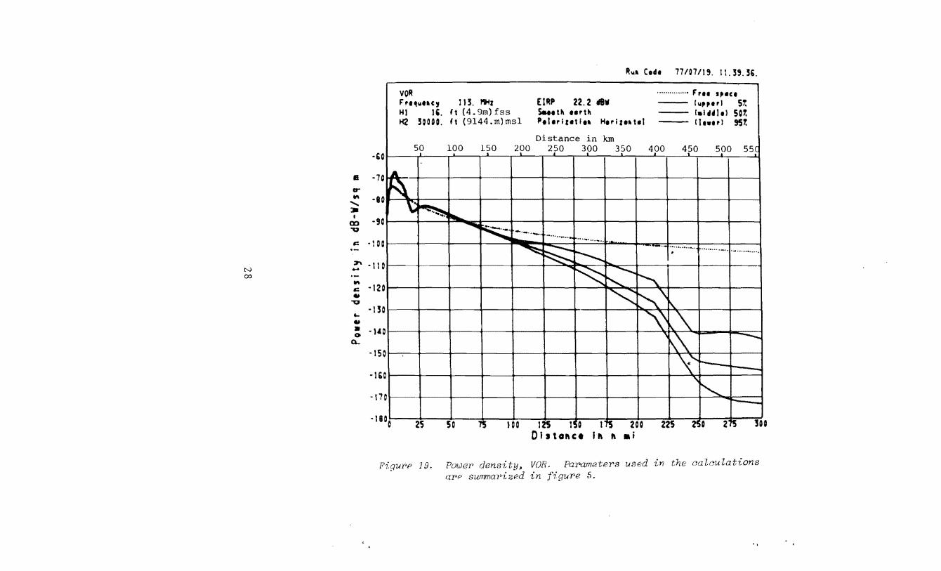
R~a Ctdt 77/07119. 11.39.3&.
VOR ··············· r,., .... ,. r,,~~uc, 11!. I'Jofr ElRP 22.2 d8W ~~ .... .,, 51. Hl 1,. ft (4. 9m) fss S..ttll tertii l•lddhl 501. H2 30000. ft (9144.m)msl Ptltrizetlta Htr i ua tel lhwtrl !51.
Distance in km 50 100 150 200 2?0 3po 3~0 400 450 500 55f
I ·&0
&
rr II'\
......... :a
I co "0
.: -N
:n ():) -·-II'\
.: ., "0
... ., a 0
a.. • 15
lA
f'\ I f• ~ .. ... ~ ........
....... ~
. ..... -~ .......... I
... -·····-··· -~·- .. ~ .... ~ ~
···-· ~·~··· .•..•.. ••••••n•-••
~ • ·-••••••~u••
)
~ -............
) t'-. ~
"' ~\ ' '\' ~'\ 'r\'\ --.....
I
\' r-- -I "'
·70
·80
·90
·l 0 0
• t t 0
·120
·l!O
·140
·I&
) ~ ..... _ ·17
·It )0 25 so 7S )00 t2S 11 D ITS 200 225 2' D 2~ lD 0 0 J I tOI\Ct II\ ft ai
19. PoweP density~ VOR. PaPametePs in the calculations aPP swnma1•izPd in j'iguPe 5.

N 0
R~a Code 77107115. 22. 15.49.
TRANSMISSION LOSS. ATC ............... f:'rtt IPOCI
r:'rt1~tllcy !25. 11Hz Goi11 C.O dBi ~~'''rl 57.
Hl 50. It (15.2m) fss Sauth torth --- !aiddltl 5D7. H2 45000. It (l3716.m)msl. Polorizotita · Horiztlltol ---!leur! 957.
Distance in km 100 200 300 1]()0 500 690 700 I 90
00 "U
,;: -M M 0 -,;: 0 -M
~ --
~ \' '
~ )r\ ............
._ r--0"
......._,..., "- r--- ~
............ - -0 ............ ~ ~ r::::·· ~ ... ··--·· ······ .. - ..... ...... ... r, "·"'= !:-~ ...... " ~ ~ " I
'\ ['\\ 0
1 0 0
II 0
120
130
140
ISO M -&
"' ,;: 0 .... .....
18
\\ \ 0 --1--·----\ l\
--"" 0 ~
\' I'- "" 0 ~ ~ ' ""- ~
:
1&0
110
19 r-- .___ r......._ i 20
21 I. 25 SC 75 100 125 150 175 200 225 250 275 500 525 350 375 4DD
Distance in n ml
Figure 20. Transmission loss, ATC. Transmissior1 loss valuPs computed 1Jith paramet;ers in figure 1 for t;hrJP avaaab1:Uty of 5, so) and 95 pereent.

:.. en -110 'U
c:: -120 -.., -
..0
VI 0 ~
0 ·-0 > 0
.... ·170 .., • -180 0 I H n..
·19
POWER AVAILABLE, ATC Fre~~~•~c~ 125. MHz H) 50. It (15.2m)fss EIRP 14.0 dBW
100 200 300
in
R1111 Coc!t 71/Dl/18. 17. 55. 29.
S•u 1 1'1 to rtl'l Polorizotioll Horizo11tol
Distance in km
400 500 600 700
Frtt SPOCt
951.
800 900
eet (meters)
(15, (13,716) (12,192 (10, 668
(9,144) (7L620 (6,096)
5,000 (4, 572) 0,000 (3,048
I I
Oistol\ce ;,., 1\ 111i
Figu~e 21. Powe~ available cu~es~ ATC. Powe~ available c~es we~p ~ompu with pa~amete~s r~om figu~e 1.

I'!
cr If\
......... Jill
I
en v
::T\ vi .... 1-'
If\ ,;:: 4,)
v
..... 4,)
• 0
0...
- II 0
-12C
P.~o~ft Codt 77107119. 17.H.OI.
PO~ER DENSITY. ATC F'rt~ut~cy 125. MHz HI 50. ft (15.2m)fss EIRP 14.0 dBW
S•ootll tort)l Polo•izotio~ Horizofttol
Distance in krn
(1, 524' ~
.. · · F'ru ''oct 951.
(15,240 -t--+~----1 (13, 716) .. (12,192) (10,668)
(9,144)
(7,620)--+-+
(914) ~~~~ (610)-f-- ...... ~
~~~ (457) ...... §
( 305 )-(152'
-230 I ~ I I I I I I _..J_..-J 0 ?1\ c:;n ,~ I At\ 1')C:: •Cf' f '1r: .,1'1;1'1 'l""l'r' "1r'A , ...... ':IrA A """ .... ,.. ........................... alP• ........ ..
n rni
Figur•p 22. Pm.Jer> rh:msity cuPVes, ATC. Power density curoes '"'erP eompute::d with para.me::ter•s [rom f'tgure 1.
~
en "0
c:
.....
..... 0
VI c: N 0 -.....
..... -I!. ..... c: 0 ~
......
TRANSMISSION LOSS, ATC Frt1wt~cy 125. MHz HI 50. It (15.2m)fss li•i~ 0.0 dBi
I 2 0
I 30
140
150
IGO
170
180
190
Wu in feet (meters) 21 0 2 5 '000
22~ 3,000 2,000
Ru~ Code 7710&127. 1&.43.0&.
Suotll urtll Polarizatio~ Horizo~tal
Distance in km
Fru IPICt
957.
(15,240 (13,716)
.....
0,000 (12,192) 35,000 (10,668
(9,144) (7,620) (6,096) (4' 572) (3,048)
250l I ,--I : ... _,,, I I I l I I I I I I I I I I I 0 ?C: c~ .,c .,., .. ,11\,. ................. --- --- --- --- --- _ _ _ _
ift f\ l'lli
FigurP 23. Transmission loss curves, ATC. Transmission loss cunJPB were computed with parameters from figure 1.
.,
~ ...... ...... 0
"' "U iC 0
"' ::J 0
.c:. ~
t.N iC V-l
... "U
::J ~ ·-... -0
~
...... 0 ~
u ~
-<
FigurA 24.
.<
R~,~11 Code 77/0.C/1 '· 12. 27. 0 1. Facilit' Pouer ovoi !obit
VOR POtii[R AVAILA8LE VOL~.~€ .............. ·Free apou EIRP 22.2 d8W F' """' .. (' 113. I"Hz I I I I I I I I 5.001. HI 16.0 ft(4.9m}fss P•lorizati•" Horizutal 50.001. Power ovolloblt -114. d8W S..•ttl earth ----- 95. 001.
Distance in km
100 50 100 150 200 250 300 350 400 450 500 550
' •
90
80
I v I I
I
/ I I
/
30
25 I / •' I I
I
70 I J ,•' El
~
&0
50
.co
30
20
10
/ v ... I II
I I • I
'/ ... •
/ .I
' , , llr
// ~I II , v ••
// II • I I
, v ,lr , I
~,~ ••• •
~ "' . •• •• I I ,, •
~ ~ ••••• - Ia t I I tl I
0 2S so 75 100 125 I 0 1'5 200 225 250 275 Olstal\ce if\ 1\ Mi
Pou.JPY' availablf': volume, V()R. Power availabl.P vol-ume for '1 sing for• .S, 50, and 9.') per•cent time ava·Z: l-ability ur;ing the parameters
20 -~ Q) ro ;:1 .j..l ·rl -- 15 .:: tO
.j..l lH llj l--1
10 u l--1 ·rl A:
5
30 0
{XJI"Wr avai tab f·igure 5.
VI .r.:.
Rua Cedt 71/0.C/19. 12.27.27. F'ocilit!f Power dtuity
V~ PO'IIER DENSITY VOLI,t( ............... r,., .,.u EIRP 22.2 d9W Frtf!u .. cy t t'5. !'tit t II It til 5, 001. Hl 16.0 ft{4.9m)fss Peloritetiea Htriuatol 50.001. Power deasity ·111.0 dB·W/sfl • S..eth terth ----- 95. 001.
Distance in km 50 100 150 200 2:0 300 350 400 450 500 55? I I • 1 00 ... - / v I
30 - 90 J 0
.,.. "U
I I I I
I I 80 25 ~ a .,.. :J 0
.c. ... ~ ·-.,
"U :J .... ·-... -a .... -a '-.., '-·--<
5
I IT ,~
J I • . •' / I I
I, v 1 .. I •' I ••• ,
I
'/ •• , •' ,
I , •• , ,r // •• ~· •'' I , v • I"
~'/ I I
I I
D I
,' v I lp
,/ • •• 0 •• I
~ I I •• , •• •••
0 ~' I I
~ ~ ... I tl •
- •• lo 25 so 75 IOC 125 ,. 0 t 'S 2DO 225 2!0 215 lO
70
GO
.. l
2
~ 20 .~
Q) '0 ::1 +l ......
15 ~ l1l
+l 4-l l1l
10 ~ ~ . .....
I<(
5
0 Olstaftct 1ft ft •i
Figu~e 25. Power density volume, VOR. Powe~ density volume fo~ a single power density value availability using the pa~amete~s in figure 5 . for 50, ar0 95 pe~cent
. .

VI tf1
100 --- '0 0
M '0 80 c:: a M :J 70 0
.c. - '0 c:: -41 so '0 :J -·- .co --a so --a ... 20 u ... -< 10
0 g
R~ Ct4t 77/0.C/1,, 12.27.5'5 Feel! It~ Tr•nlultl l•n
V~ TRANSI'IIS ICtJ LOSS VCX..IA'( ............... F'ttt •P•c• ,.,. 0.0 dBi F , ....... ~, 11'5. l'tiz I I I I I I I I 5, 007. H1 16.0 ft(4.9m)fss Pel•rlzetlll Htriaeat•l 50.007. Ttaa,.latlta less 1'S.c. d8 S..ttll ••rUt ----- 95. 007.
Distance in km 50 100 1~0 200 250 300 350 4~0 450 500 ssp
/ L .~' I v
I
J I I I
I ~·· / I I 1 ..
I II
II I
..1 ·-..,l_j_ lr II
I I
' II
,' v II ,,.. II _..· ·-v ... ~ •• ...
~' _.. ··-,'/ ·-•• •• II
,;/ II •• •• I I
I I
-:P:. I I•
~ I I
... ~ ,
• • . I I I
~ ~ .. I •••• .......,
25 so ~~ 100 125 11 0 1 '5 200 225 2!0 215 '!0( Otstat~ce It~ " •i
30
25
.Q c
20 ·ri
(!)
'0 :;j -I.! ·ri
15 .:: Ill
-I.! 4-l ~m
~ 1--1
10 ~
5
·ri ~
26. Transmission loss volu'!le, VOR. Transmission loss volume for a single transmission loss vaLue for 5, 50, and 95 percent time availability wn:ng the parameters in FZ:gure 5.

.... --0
"" -,;, ll:! 0
"" :::J 0
.c. (..;~ ..... 0\
ll:! -., -,;,
:::J .... ·-... -0
.... -0 t-u t-
·--c:
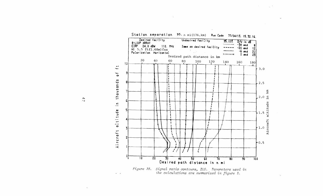
R~n Codt 17/01/15. 22.57. 55. Facility 95. 007.
llS ElRP CONTOURS ............... Po .. r dnsity -lf I. 0 dB-W/s~ • Frt~~<ncy I U. MHz ........ HI 5.5 ft(l.68m)fss Polarizotiu Horizontal
S•ooth tar th Distance in km
20 40 60 80 100 )r---
I I v I
I I
1 0
I I
1 I I
: I I : I
I • I l I . I I I •
I . I I
I I I I I
I I
I I I I I • I I
i . I I
: I 1/ I I I I I I
• I I . ..L ' i .I I
1/ I I • . I I I ; I I II
I I
; l' .. ··I . i I I
• I
! • ~
I II lw I I . I I • i I • I I • II
' I I • . \ ·. I'
I ~ ) ) .• • ) , . I I •'L
, I • ~
, I !' I .. . ·7 , .. . . , , , .
I ./ . ,
9
8
7
G
5
4
!
2
0. --I C 20 !0 40 Distance
50 &D in n mi
-----120 140 _, ~·
I
I I
--70 -. 80
ElRP ·54 n4 0 ·20 a11d ' ·10 nd I 0 ·& alld 20
160 180 __ L ___ __L ..
I"
r
i
'0 IOC
3.0
2.5
1;1 c:
2.0 ·..-!
(l)
'd :;1 .j.J ·.-I .j.J
1.5 .-I n1
.j.J 4-l
111 1-l u
l.O 1-l ·.-I ~
0.5
27. EIRP contouPsJ ILS. EIRP contouPs aPe shown in the a tude vs. distance plane foP a 95% time availability and the paPametePs of figuPe 2 .
..
(,A
'-1
.... ....... .......
0
..., "'0 c a ..., ::I 0
..c. .... c
II)
"'0 ::I .... ·-.... -a ....
....... a ..... u ..... ·-.-.::.
Ru11 Ctdt 77/04/08. 14. 35. 55. Foci 1 it¥ 95. 007. EIRP
TACAN ElRP CON OURS . ·············• 24 n4 l9 Po11tr dt11sity ·8b.0 d8·W/s1 • Fre1ut11cy 1 tSO. ttlz I I I I I I I I 23 ad .42 HI 30 ft{9.1rn)fss Po 1 or i u t i 011 Vertical '50 nd 45
S.ooth earth ------ 'SG nd 48 Distance in krn
50 100 150 200 2~0 300 350 400 450 500 550 • 100
2
I : • I I I I
~~· : I I
I
V/ ··-: I Lt
I II J I
I ~I i ·---I lw
/"' I i I I , • / I l • I t--
I I. ~ I ~ ! • i I
/ I
I
• I r•., I I .· •• I /L' •• .· • I I I .. I : I I I I I / J' . I ~
I i / .~'/ I • j • I I • I / ... . • I I • I .. _
....... ·~ ...... : l I I ... / " I I ./ ~··· /
I
' ; I
I ' ' ,
I
: r I I ,.l •• v,., : . I I fl ! '
I I I
I ' •'I ./ ~' . . I •
r I ,i
,
~ I ·' • ,. .. ""' • • J
, ~· •''../ ! J. ..A" ,
90
eo
70
': sc
40
30
-I v/. 1/ / ~ ..,. ...
~~ ... ,_ ........ ·~ 25 50 75 100 125 11 0 175 200 225 ~0 215 ]Q •
Dls\al\ct '" " 1111
a
30
25
12 c
20 ·rl <J)
'0 ::J +' ·.-I +'
15 ..-i ((j
+' ~ ((j H
10 ~
5
•.-I ,<:(
Figure 28. F:.TRP contour•s, TACAN. ETRP contours are shown ,·.n the altitude vs. distance plane for a 95% time avaUabili b; and the parameter>s of figure 4.

lN C:>
Ru~ Codt 77107/12. 20. !2.00. F" CIC i I i t !I 95. 0 07. E~RP VOR EIRP CONTOVRS ....... """ ~ Q nd 2: Power dusit!l • I I I. 0 dB- 'II s 'I " f:" rf'!llt~C!j ll'S. MHz t I t I I t I I 5 nd 25 HI IIi. 0 It (4.9rn)fss Polodutio~ Horizo11tol 10 llld !C
S•oo t h eo r t h ----- 15 CillO 55 Distance in kro
..... --0
.... -o ~
0 .... ::J 0
s;;. • A
~
u -o
::J ... -..... -0 .. -0 ... u ... ·-<
50 100 150 200 250 300 350 400 450 500 550 : I I .. ..... ' ' I ' I ' ' I ' ' . .
: : I I .... ,r
V~ .
1 .. ·· ' . .
' / . ' ' .• v I ..... . / ,' . I .
~ . I . . .... . ~ .
j I . ~
: . • I ··· ...
I J ,, .... . v ~
·-. J . . ./ I'··· .. . If ~ .
/ . ~ )·-- . . ~
I ~ ... v ·" ~ . , . J .· ~ . Dr--- . J ~·.' •' L 1~
•• L' ..... .. ' v~ " . I ~
' I • . .~' '
' . .· : .· v _; " !_...... '
~ ,..
• ' ~ ... . , ,. _ ...... •• . . . "'
. l'/ " ~ .............. ~
,' ' " ,..
•• / . ,' .. ··· ,• ~ ;---· • ~v ,/ L··· . ...- ,• • V, .. ... ' . ~ . ... .. ,, ... . ,
1---
~ v ,·" .. · ~
... ... ~
. • ... . ... ~ .
1 c c
90
80
70
GO
so
,, 3/1
" 111
30
25
~ 1: . ...
20 Q)
"0 ::l .j.J ·.-I .j.J
15 rl Ill
.j.J 4-1 Ill ~ 0
10 ~ .... ,.;(
5
0 25 50 75 100 125 150 175 200 ---225 --250 . 275 300
Oistol\ce il\ 1\ Nd
Figu~P 29. EI~P contou~sJ V0R. EIRP contou~s a~e shown in the altitude vs. distance pZanP for a .9,~'h t£me availability and the parameters of figure 5 .
..
..... --0
"' "0 .: 0
"' ;:J
0 .s::. -
u~ .: <..:l .,
"0 ;:J ... ·----0 --0 ... u ... ·-...:
FiguT>e 30.
R~~ Ctdt 77/07112. 20. 5A.A8. F'ocility ~5.007. Power Available in dBW
T~C~N POWER ~VAILABLE CONTOURS ............... ·100 nd ·Ill EIRP 5!. 0 d9W FPt1~t11Cy 1150. I"'H: . II..... ·I 0' 1111 d • liS HI 30.0 ft(9.lm)fss Ptlorizatiu Vertical -10& llld ·118
Sauth taPti\ ----- •JQ!) Olld ·121 Distance in km
50 100 150 200 2~0 ;300 350 400 450 spa 550 I .. I I . I ,' . I .
: • . . . I ' I . • ---
~ I ...... / I . I .
/ I . ) r----~ . I ---- .. I ,'r v I I . I . I . . I
/ • . I ~ . I .
-~ ~
1/ I // ~' .
I _: . ~ . . / . I . ~ 01--- .. - .
' .. - .'' v , :
J I . ~~ .
I . . I . . _f . I . lr---~ .· I I . '/ ~ . .
~;' ........ ' ~ • 't I " . 0---,___ --- : .
' ;
-... // r ....... . . ,•'/ ~,
i ' / . ' ' ~
Or- ; . I /
.... / ;I .... . .. v /_. .~·/ I
0 I
' , ... / •·.. v _,~ __ .... . •' .. u;, .,"
... ·:/-<· •• v : L ~ ...
.... · .. v .. ~:··~ ~ .... •• <II! .: . .t ..................
100
~0
80
70
GO
50
AO
50
20
30
25
12 >::
20 •.-l
Q)
'0 ::I .jJ •l"i
15 ~ <\1
.jJ 4-1
<\1 ~
10 ~ •ri ~
5
I -- -0 25 so 75 I 00 125 ISO 175 200 225 250 275 300 Oistar.ct ir. 1'\ Mi
PoueT> available contours, TACAN. PoueT> available contouT>s aT>e shoun in the altitude vs. distance plane for a 95% time availability and the paT>ameteT>s of figure 4.

'""" 0
.... --0
VI -g c: CJ VI ::;, 0
..c. -c:
"" -g ::;, .... -CJ --CJ L.
u ._
<C
Ru~ Cod• 77/QA/t!. tO. 10.2' Facility
TACAN POWER DENSITY CONTOURS EIRP 39.0 d8W Ftt~utftcy ltSO. HHz
Polarizotioft Vtrticol S•ooth torth
95.001. p, •• , OtAII\~ ............... -77 ..... ·8, ... 1 .... -eo ... ., ·!2
Hl 30 ft (9. 1m) fss ·83 ncl -ss ----- ·8G llllcl .,.
Distance in km 150 200 250 300 350 400 450 500 55~
1001 I I I ; ! I / /" v .r t-30 I I I I ' ' ' I 90 I I I I : • l ! • ) I I I
I I I I : : I I : ,.··; 1/ • I • • I I I I .
1 I / • I 25 eo · • •
50 100
1 I / 11 I ]
I I l I : r I / / .. r v v I 0
I : 1} I 701 I I : • : •
I I I I : I !/ ,' ./ II I / . 20 -~ I 1 1
GD'---' I I: .: o1
I ~ I I I 1.: • I / / .'' / ::l
5
I • I / I +J I I .•· II , ·rl
I I I : / / I / +l
so I I I ! : I I / I. v . I 15 ';ri : I I . • I ~ • . •• . +l
I l I : •' 1 ./ ,• ., Lj..j 40 I I I / •• v I ...... •''/" .,' ~ ! I I ... .• . / u ' I l I i •' I I / I I 1 0 -~
301 J 1 : _rr/ .. · 1• 1 <( I . I ~ •• I
i l/ ,.. 'I J 20 1 1 1 1 .~ ,· ./ ' 1
/ _, I I I l I I ·1 I I/ .~ ' ··· ~· )_ ,'
• •/ I •' I ' . / / ... ...,, I o 1 /
11 11 •• •••• • • /. ...,., 1 I l I I I I 'I /' .•'V , : ... ~~· I
··~···.:: ~~ k:.U............., 1 I I I I J
25 50 75. 100 125 · tSO 175 200 225 250 275 300 0 i s tal\ c e i 1\ 1\ rwd
co
Figu~e 31. Powe~ density conto~s, TACAN. Power density aontou~s a~e shown in the aLtitude vs. distance pLane for a 95% time avai lity and the parameters of fig~e 4 .
....
.p. 1-'
Ru11 Code 77/0'11'5. 10.17.:2.
r ac i 1 it~ 95.007. Trou•initfl !tu TACA.N TRA.NSMIS ON LOSS CONTOlJ'R ............... 125 Ofld lotS Goi11 0.0 d8i Fre~tuti\C!t ! 150. 11-iz I I I I I I I I 130 01\d ISO HI 30 ft(9.1m}fss Polarizotio11 Vtrti col 135 01\d 1&0
S.ooth torth ----- !.tO ol\d 170 Distance in km
100 --50 100 150 200 250 300 350 400 450 500 550 .
.' I I 30
- 90 0
11"1 ""0 eo
..::: Cl 11"1 :::J 70
/ : / L I I I I I
I
I I" v I I I
: I
I I I
25
s ..1(
0 ..c:. - bO
..:::
4U 50 ""0
:::J - 40 ---Cl
30 --Cl ..... 20 u ..... -~ 10
0
I .I I I
... 1 I I I
I --~ : .· ... ' I
I , I
I I • ... I I ... I
I [l"
/ ,' I l • ,
I I It Ia I I I ... II ... ...
I If : I v ... : •• 1
, • l , I • I : I , • .,'
f I i ,. "' .. l • " I •
/ .,. ...
·' ··· ... I .· I , .. ~r J / ,•' , .. v .. ~ ••
~ ., ...
! / ' ' •• ,. .. I I .•
! ' ~// .··•· .. ... v-·"' ~ -~,~ /... ,, ·~.J,<r~ . -
) 25 50 75 100 125 11 0 1 5 200 225 250 275 30
20 .s (]) "fj ::l .jJ •.-!
15 ;:: ((!
.jJ Il-l
t"O H
10 u H
•.-! ,:(
5
Distance in n Mi
FiguPe 32. TPansmission loss contouPsJ TACAN. TPansmission contouPs aPe shown in the altitude vs. distance plane fa~ a 95% t·Lme availabilityJ and the pa~ametePs of fig~e 4.
Du ired dis ta11ce 100. n mi (185. km) R~~ Code 17/0(/19. 12.22.(3. Otsirtd facility
VOR SI~ RATIO-S Vlldesired facility ............... Fru space
HI lG.C ft (4.9m)fss Soae as desired facility I~,.,. tr I 57. H2 30000. ft (9144 .m)msl l•iddlel 507. Fre41J~e11cy ::5. I'Ht llowerl ~7.
Station separation in km
) 100 290 300 400 500 600 700 50
I 40 )(/~ m "'0 lh r; ) 30 .: -0
·-+:.. -N
a '-
-a .::.
~ /I I
~ ~ y
I / / ~
........... ... ~ .....
~ •······· ·····-· ········ )
20
10
0 0'\ -..,
::> ........ 0
··;; iii' ,..· I ,. I ,..
/I ~ I
·1 0
·20
·3 0 v •
·.C 00 25 so 7S 100 t25 ISO t75 200 225 250 275 300 325 !! o r~ .cc a Station separation in n mi
Figure 33. Signal Patio-S~ VOR. DesiPed-to-undesiPed~ D/U, signat Patio vePsus station sepaPation cuPVes aPe shown foP a desiPed facitity-to-PeceiveP distance and time availabilities
5, 50~ and 95 Bot~ the desiPed and undesiPed stations have the paPametePs vf figuPe 5.

.j:::..
(.A
m "0
c: -0 ·-.... a ... -a c: lin -....
::;, ....... 0
Stotio11 uporotioll 250. n mi(463.km) Ru11 Codt 17/07/U. 00.31.01.
On i rtd foci I it~ Vlldtsirtd focilit~ 1 VOR SI,NAL RATIO·OO ............... f: Pit I !IOU
HI 1&.0 ft (4.9m}fss So•• os duirtd focilit~--- lu1111trl 51. 1 H2 30000. It (9144.mlmsl l•ldd!tl 501.
f:rt .. uiiiC~ 113. MHz n ... ,, !151. Desired distance in km
50 1qo l~Q 2(\0 250 300 3(0 400 450 I • __.___
- \ .\"' ~~ ~
(''' .......
"''\ ~ l ,,
'• ·•·· ..... "" ~ ···· .... ' ··•·· ........
~ .. .... ~ ........... ['....
"' ~ K"··· ... ··•·····
50
AO
30
20
I 0
0
·I 0
" ~ .... .
·· ...• ['.. ····, .. ·20
·3 '\ ~~
.. '• .. ..
!"'- '
·.& I -~"' ~"'\ I ·5.0 25 so 75 1 0 0 125 15 0 I 75
Desired distaftce ift ft Mi
I"'\ 1\ --200 - --225 250
Figu~e 34. Signal ~atio-DD. VOR. Desi~ed-to-undesi~ed. DIU. signal ~atio ve~sus desi~ed lity-to-reoeiver distance ou~ves a~e shown for a fixed station separation and time availabilities of so. and 95 percent. Both desired and undesi~ed faciUties have the parametel'S of figure 5.

..,. ..,.
D/U 23 dB for 95% R11ft Ctdt 71/01122. 13. 4\. 4.&.
Ouirtd lo,iJity Vnduirtd h(i)ity ............... 0 _d•l:l•t2 0. S-LOOP ARRAY Hl 5.5 It (l.68m)fss Soat as dtsirtd lo,ility ----- ~c. ud ISO. H2 4500. ft (1372.m)msl &0. Gild uo.
• ' • '. ' l • so . Facility separation in km
.., ., .,
.... 17'\ .,
"'0
.c -., -17'\
.c a ., .c ·--., .., .... :::J 0 y
"'0 ., .... -.... .,
"'0 .c :>
12
20 40 60 80 100 120 1<10 160 180 200 220 240 I _L I • I . .l I • i/ I ) 1.' ,, . . ;
I ~-
/I ,' .' . ~~-~ [,/ • I . . • --
/,' :·· • • I l ~-
. I
I " )- 1---- I I . ( F
~\ i ' I \ \
I I '· ..
'\ . ,. ·· .. . 1\ ' ...
) 'II ,· .. ~ · ..... .
I \ \·: . =
,, I \ ·. • I : ;; . . ,. .
0 I
/~ ,' / I
/i / • . 0 . .
V/ I. v / L· I .
I I I / I
i I ;
[\\ .. . \ ·.
I . \ ·.
. '\_I·. I 1\ '\ t··~ 'II I i\ ··· .... I • \ \\ ~\ ....
I
\ '· 0 I I ~: -- -. -. ..
3GO
330
300
270
240
210
l8C
150
!
b
3
0 I 0 20 ~0 50 40 GO 70 80 90 100 110 120 130 140 Facilityseporotion inn Mi
Figure 35. OPientation, ILS. Facility sepaPation needed to obtain a D/U of 23 dB foP a time availability of 95 pePcent is provided as a function of undesired (ordinate) and desired (line code) course line angles (fig. 43). PaPametePs for both the desired and undesired facilities are as given except that the aiPcraft altitude is 4500 ft (13?2 m) msl. See page 61 fop discussion of critical protection points.
.... --0
.., 'V c:: 0 M :I 0
.c. .... +>-V1
c:: ·-... 'V :I .... .... -0
.... -0 .... ..., .... ·-...::
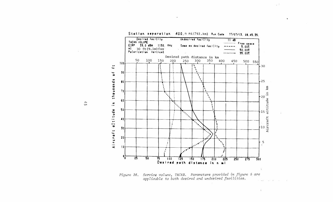
Station separation 400.n mi(74l.km) R .. 11 Code 77/07113. oa . .c5.S5.
Ouhed foci I i ty Vlldtsired facility II d8 TACAN VOLUME , .............• F'ret ,tee EIRP "· 0 d8W 1150. MHz So•• as desired facility ----- 5.007. HI 30 ft(9.lm)fss 50.001. Polorizotiu Vertical t I I I I I I I 95.001.
Desired path distance in km
I 0 0 50 100 150 200 250 3?0 350 400 450 500 550 • . .. _,___....__j_
I~ I \ . \ . ' I
90 1\ • ' 1---- -~
eo
70
&0
50
•o
so
20
1 a
00 25
F1.:gur>e 36.
\ ' I
' I
' • . \
•• \ • • ' • . \ . \ \
I . \ . \ • . : \ ..
\ I ~. I : ·. • \ \ ---•• l\ \
• . II
I \
.. 1.~ ·-\ .i II
~ \ .. I •
··:1 I ., I . \ I ' v ' I' ' ; •• \ I I ..
\
~ .... . . •• 1 I i •
j i 50 15 I 0 Q f25 IS 0 175 200 225 250 275 soo
Desired poth disto~ce in n ad
Service volwne~ TACAN. Par>ameter>s pr>ovided in figur>e 5 ar>e applicable to both desir>ed and undesir>ed facilities.
30
25
20
~ s:::
•.-I
(!)
'd ;::l .j.J •.-I .j.J
15 ';ri .j.J 4-l l1j ~
10 ~
5
·.-I r<:C
... --0
... ~ c: 0 ... ::J 0
.c. ... -!>-0'1
c:
.. ~ ::J ... ·---0
--0 L.
u L.
·-oe:
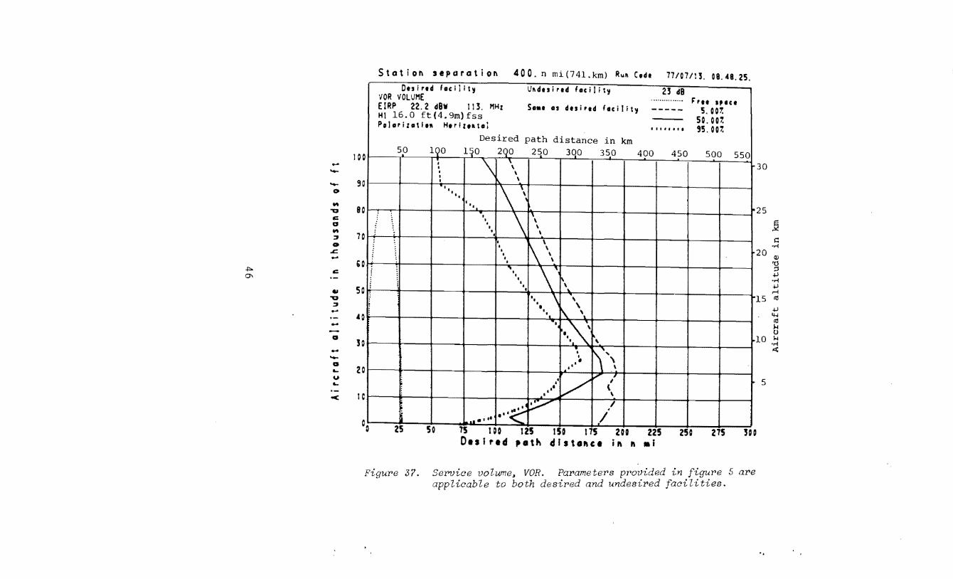
Statio!\ separatiol\ 400. n mi(74l.km) Rllll Code 77/071!3. 08.48.25.
Oulrtd faciiit' Ulldttirtd facilit' 23 d8 VOR VOLUME ••a.•·········· F'ru tPICI EIRP 22.2 d8W 113. MHr Sa•• at desired facilit' ----- 5.001. HI 16.0 ft(4.9m)fss 50.001. Polariratln HtriUIItal I t I f I f I • 95. 001.
Desired path distance in km
) 50 lQO liO 2QO 2~0 3QO 350 400 450 500 550
I \ \ • . \ I \ I I ··, \\ I I I
I I I
• \ 1\ I I
\ • I \ I
• \\\ . . I
• I . • '\ \'· •
1', • • . I • -..
'• \ \ I \ I
I I I I\ \ I
I·~~\ \
""
100
90
80
70
GO
so
.40
JO
30
25
~ t:
·.-!
20 Q)
't1 :;1 .;.J ·.-! .;.J .-l
15 <l1
.;.J 'l-1
<l1 1-4 u
10 1-4 ·.-!
2
...
\'\ I • •' ... .:c
I ·v k-"" / II \ I \ I
5
~ I ~~
. : •• I I 'ol. I tl
0 25 so 7S I 00 125 ISO 175 200 225 Desired 'ath dfstaftee ift ft •I
250 275 SOD
Figui'e 3?. Service volume, VOR. Pai'ametei's pPovided in figui'e 5 ai'e applicable to both desiPed and undesired facilities.
..
1 0 ! ----- I 9 0
"' -o 8 c:: a
"' ::I 7 0
..c. .j::. ..... '-1 b
c:: -.., 5 -o
::I ..... ·- 4 ..... --a
3 ..... --a '- 2 u '--
•:C
oc
Statio!'\ !Separatiol'\ 95. n mi(l76.km) Ruft Code 11/04/ll. 15. l2. IG. Desired facility Undesired facilit~ 95.001. 0:/U ill d9 9 ·LOOP ARRAY ··············· ·34 Olld 8 EIRP 24.0 dBW 110. MHz Sa.e as desired facilit~ ----- ·20 Olld 12 H1 5.5 ft(1.68m)fss _, 01\d 2J Polarization HorilOIItal
I I I I I I I I 0 01\d 23 Desired path distance in km 20 40 60 80 100 1~0 1~0 160 180 I
I I I I
I I I I
I I : I
I : ~ i • f • • I I I I I I
1--I I : : I I I I • • I : I
I • I
if i : I I I I I ,.. I • l • I ; I I I ~ ~ : j I I
I I I I I • I I I I
I I i : .. I I • I • : I I • • I
I ; : I • ~ I
I I • • ~ \ I I I 1-I
~\\ i i I .· • . . • .. · \ I J I .... · \ I
II~ \
! I I ... ~
\ ... I .. ""
. \ , ! I j I
I I :r I I 1/ I I :
II II , ~-' l i
.. 10 20 30 40 50 GO 70 80 90 100
Desired path distal'\ce il'\ "Mi
F1:gur>e ,7,8. Signal r>atio contour>s> ILS. Par>ameter>s used in the ca leu lati.ons ar>e swnmar>ized in figW'e 2.
3.0
2.5
s .:.:: 2. 0 s::
•.-I
Q.)
'0 ::I +J ·.-I
1.5!:: Ill
+J 4-l Ill
1.0 ~ u ~
·.-I ,:t;
0.5
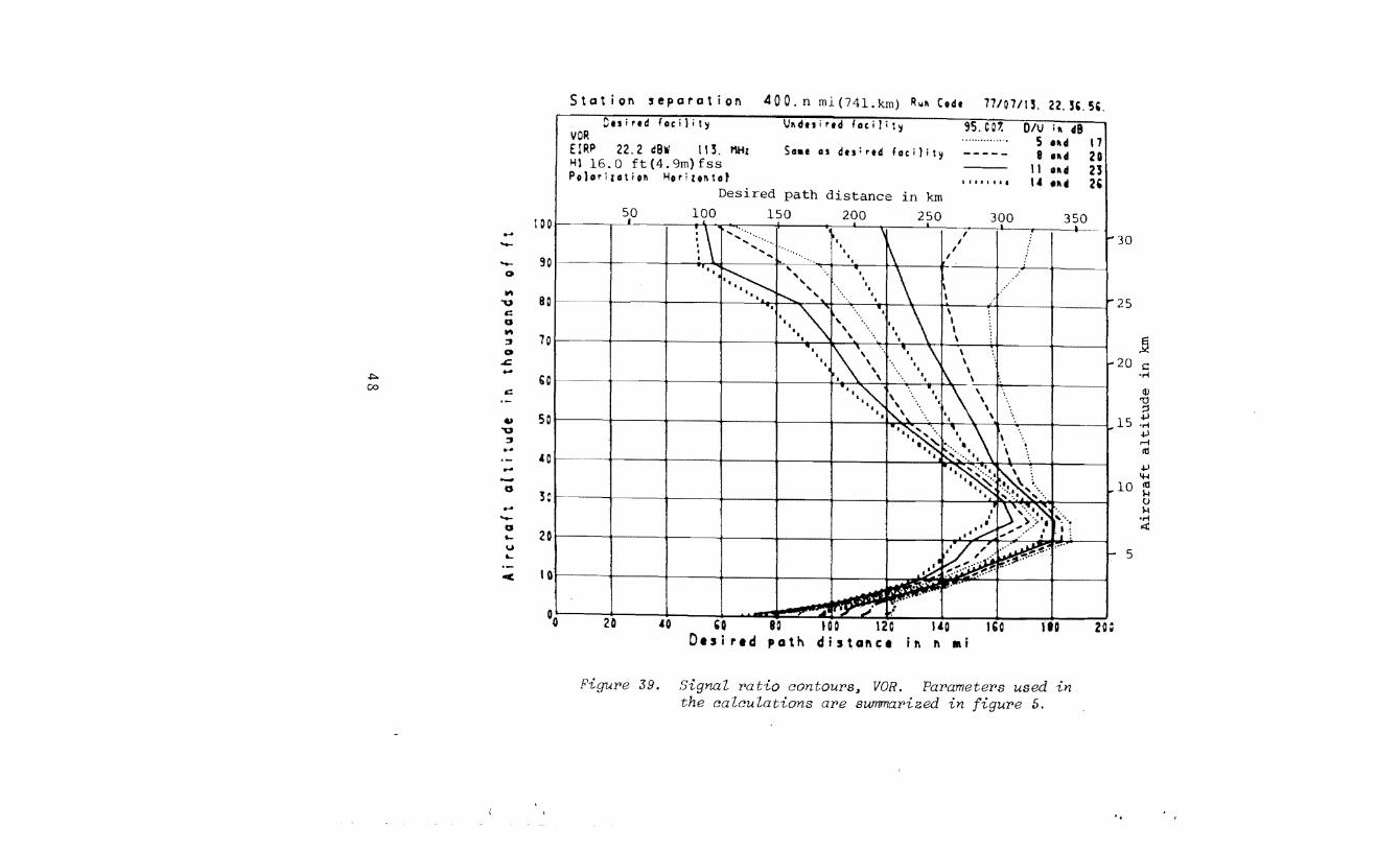
---0
M "U c: a M :J 0
.c. ~ -co c: -..
"U :J -,_ .... -a .... -a .... u .... ·--<
Stat ion separation 400. n ml(74l.km) Ru11 Code 77/07115. 2Z.K5t.
Du i rtd foci I it 'J II OR EIRP 22.2 dBW 113. 11tiz Hl 16.0 ft(4.9m)fss Polorizotioll Horizo11tof
Vlldtsirtd facilit'J
Saae as du<rtd foci)it'J
Desired path distance in km
100
' ' ' '
150 200 250
95.C01:
-----l f t 1 t I I I
OIV ;, cl9 5 ud 8 Ud
II ncl II •11c1
17 20 23 2'
f--'30
25
.Q 20 c
·..-I
(!) "0
B L_ ____ _j ______ ~------~------+------1r-----~~~~lr~~~t:~--~r------r15 ~ ttl
.jJ 4--1
10 ~ 0 ).I
•..-I
"' 1- 5
·1. l I I .. l .. J~·· I 00 20 40 GO 80 \00 120 140 1&0 180 20~
Otsirtd path distance inn ai
Pigur>e 39. Signal r>atio contour>s, VOR. Par>ameter>s used in the calculations ar>e summar>ized in figur>e 5.
. .
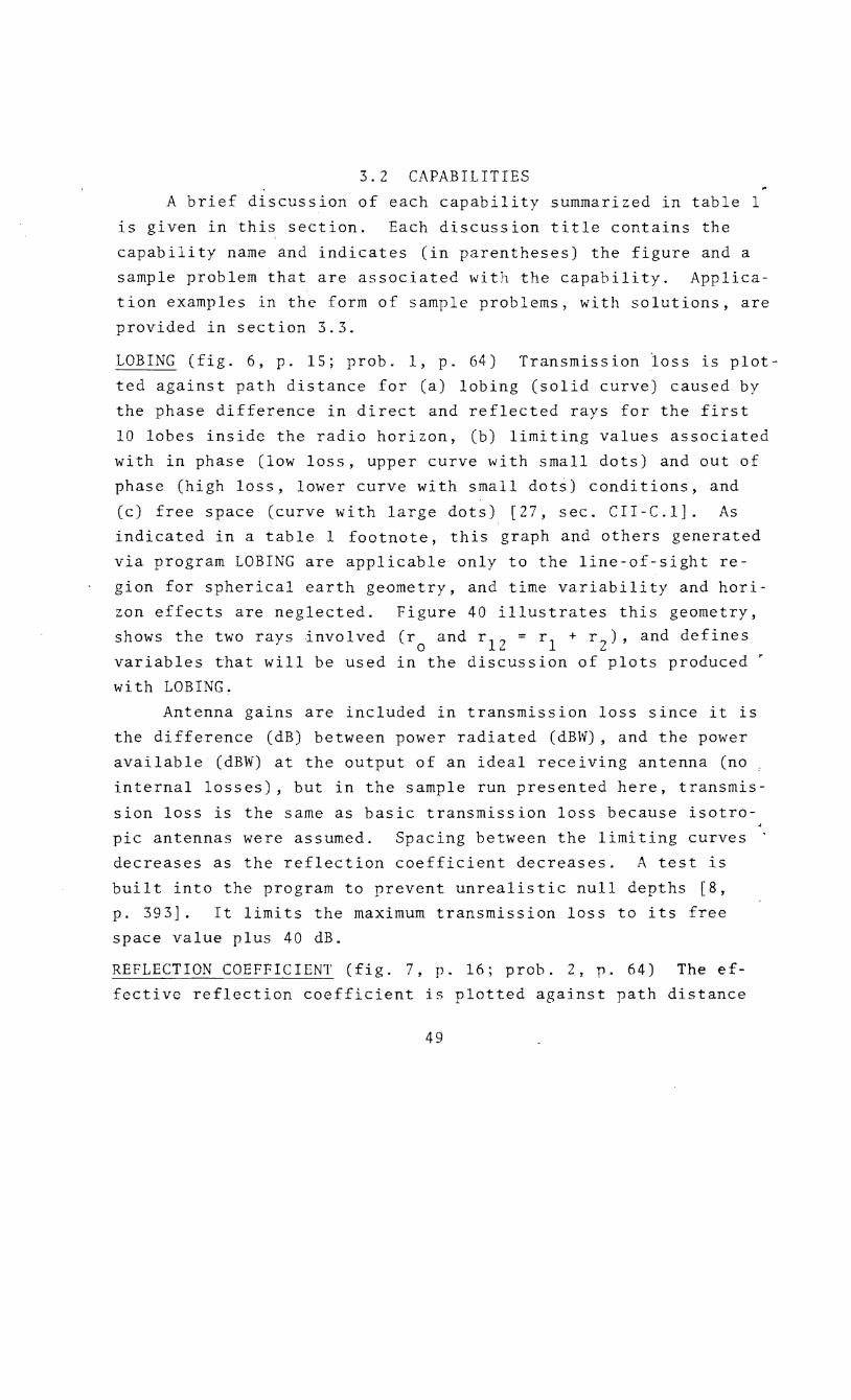
3.2 CAPABILITIES
A brief discussion of each capability summarized in table 1
is given in this section. Each discussion title contains the
capability name and indicates (in parentheses) the gure and a
sample problem that are associated with the capability. Applica
tion examples in the form of sample problems, with solutions, are
provided in section 3.3.
LOBING ( g. 6, p. 15; prob. 1, p. 64) Transmission loss is plot
ted against path distance for (a) lobing (solid curve) caused by
the phase difference in direct and reflected rays for the first
10 lobes inside the radio horizon, (b) limiting values associated
with in phase (low loss, upper curve with small dots) and out of
phase (high loss, lower curve with small dots) conditions, and
(c) free space (curve with large dots) [27, sec. CII-C.l]. As
indicated in a table 1 footnote, this graph and others generated
via program LOBING are applicable only to the line-of-sight re
gion for spherical earth geometry, and time variability and hori
zon effects are neglected. Figure 40 illustrates this geometry,
shows the two rays involved (r0
and r12
= r1
+ r2), and defines
variables that will be used in the discussion of plots produced r
with LOBING.
Antenna gains are included in transmission loss since it is
the difference (dB) between power radiated (dBW) , and the power
available (dBW) at the output of an ideal receiving antenna (no
internal losses), but in the sample run presented here, transmis
sion loss is the same as basic transmission loss because isotro
pic antennas were assumed. Spacing between the limiting curves
decreases as the reflection coefficient decreases. A test is
built into the program to prevent unrealistic null depths [8,
p. 393]. It limits the maximum transmission loss to its free
space value plus 40 dB.
REFLECTION COEFFICIENT (fig. 7, p. 16; prob. 2, p. 64) The ef
fective reflection coefficient is plotted against path distance
49
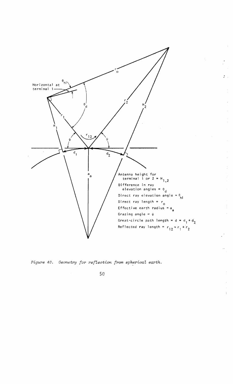
Horizontal terminal 1----~~
Antenna height for terminal 1 or 2 = H
1,2
Difference in ray elevation angles = ed
Direct ray elevation angle = e hi
Direct ray length= r 0
Effective earth radius= a a
Grazing angle = w Great-circle path length= d = d +d
1 2 Reflected ray length= r
12 = r
1 +.r
2
Figure 40. Geometry for ref!eetion from sph~ricaZ earth.
50
(d of fig. 40). Relative antenna gains, surface parameters (di
electric constant, conductivity and roughness), frequency, and grazing angle (w of fig. 40) are included in the calculation of
effective reflection coefficient [27, sees. CI-D, CII-C.2]. The
drop in reflection coefficient at short distances is associated with the ray length reduction factor [27, sec. CI-D.S]. The drop
in reflection coefficient at the far distances is caused by the divergence factor [27, sec. CI D.l].
PATH LENGTH DIFFERENCE (fig. 8, p. 17; prob. 3, p. 65) The ex
tent c~r) by which the length of the reflected ray (rl2 of fig. 40) exceeds that of the direct ray (r of fig. 40) is plotted
0 against path distance [27, sec. CII-C.3]; i.e.,
t:.r = r 12 - r . . 0
(2)
This equation is not actually used to calculate t:.r since it in
volves the difference of two, large, nearly equal terms. The formulatiori used [24, fig. 16] avoids this precision problem.
TIME LAG (fig. 9, p. 18; prob. 3, p. 65) The time lag of trans
mission via the surface reflection path relative to the direct path is plotted against path distance [27, sec. CII-C.4]. This
is the (free space) time (T) required for a radio wave to travel
the path length difference (t:.r) of figure 8; i.e.,
T [nsec] = 3. 34 [nsec/m] ~r[m]. (3)
LOBING FREQUENCY-D (fig. 10, p. 19; prob. 4, p. 66) Lobing frequency with distance (fd) for an aircraft traveling directly toward (or away from) the facility may be determined from values of
normalized distance lobing frequency (NDLF) read from this graph, radio frequency (f), and the magnitude of its velocity (Vd); i.e.,
fd[Hz] = NDLF[(Hz/THz)/kts]f[THz]Vd[kts], ( 4a)
fd[Hz] NDLF[(Hz/THz)/s mi/hr)]f[THz]Vd[s mi/hr], (4b)
or fd[Hz] NDLF[(Hz/THz)/(km/hr)]f[THz]Vd[km/hr]. (4c)
Note that f is in terahertz (THz) where one terahertz is 10 12 Hz
51
6 or 10 MHz, but that fd is in hertz.
Received signal level will vary with aircraft location as it
moves through the lobing structure (fig. 6) associated with the
phase difference between direct and surface reflected rays. The
frequency at which this variation occurs is called the lobing
frequency, lobe modulation frequency, or Doppler beat modulation
[11, sec. 4; 27, sees. CI-C.4, CII C.S]. Reed and Russell [47,
ch. 10] developed formulas using both lobe modulation and Doppler
beat modulation concepts to show that" ... no fundamental differ
ence exists between the lobe modulation and the Doppler-beat
modulation concepts. They differ only in the treatment of the
independent variable".
The lobing frequency (f~) encountered by an aircraft can be
estimated from fd and fh (see eqn. 6); i.e.,
f9_ 2. fd + fh. (5)
Here < is needed since it is possible for an aircraft to follow a
flight pattern such that the lobing with distance is compensated
for by lobing with height so that f2
~ 0 even though fd + fh > 0;
e.g., an aircraft flying the glide slope of a conventional ILS in
which the lobing structure is used to determine the desired
flight path.
LOBING FREQUENCY-H (fig. 11, p. 20; p~ob. 4, p. 66) Lobing fre
quency [27, sees. CI-C.4, CII-C.6] with height (fh) for an air
craft in vertical ascent (or descent) may be determined from
values of normalized lobing frequency (NHLF), radio frequency (f),
and the magnitude of the ascent rate (Vh); i.e.,
fh[Hz] = NHLF[(Hz/THz)/(ft/min)]f[THz]Vh[ft/min], (6a)
or
fh[Hz] = NHLF[(Hz/THz)/(m/min)]f[THz]Vh[m/min]. (6b)
Values of fh can be used in (5) to estimate lobing frequency.
52
:
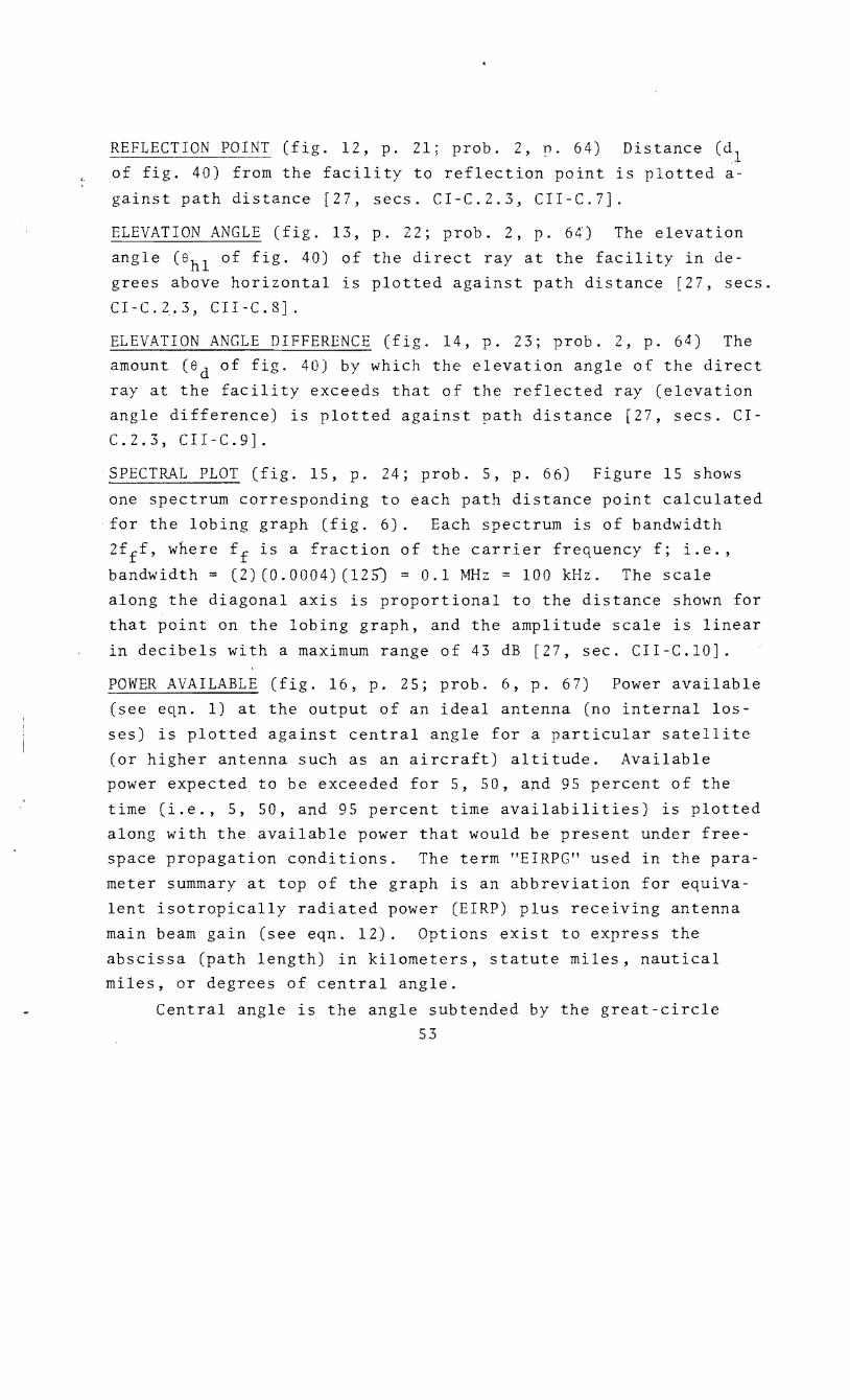
REFLECTION POINT (fig. 12, p. 21; prob. 2, n. 64) Distance (dl
of g. 40) from the facility to reflection point is plotted a
gainst path distance [27, sees. CI C.2.3, CII C.7].
ELEVATION ANGLE (fig. 13, p. 22; prob. 2, p. 64) The elevation
angle (ehl of fig. 40) of the direct ray at the facility in de
grees above horizontal is plotted aga st path stance [27, sees.
CI-C.2.3, CII-C.8].
ELEVATION ANGLE DIFFERENCE (fig. 14, p. 23; prob. 2, p. 64) The
amount (ed of f . 40) by which the elevation angle of the direct
ray at the facility exceeds that of the reflected ray (elevation
angle difference) is plotted against path distance [27, sees. CI
C.2.3, CII-C.9].
SPECTRAL PLOT (fig. 15, p. 24; prob. 5, p. 66) Figure 15 shows
one spectrum corresponding to each path distance point calculated
for the lobing graph (fig. 6). Each spectrum is of bandwidth
2fff, where ff is a fraction of the carrier frequency f; i.e.,
bandwidth= (2)(0.0004)(125) = 0.1 MHz =100kHz. The scale
along the diagonal axis is proportional to the distance shown for
that point on the lobing graph, and the amplitude scale is linear
in decibels with a maximum range of 43 dB [27, sec. CII-C.lO].
POWER AVAILABLE (fig. 16, p. 25; prob. 6, p. 67) Power available
(see eqn. 1) at the output of an ideal antenna (no internal los
ses) is plotted against central angle for a particular satellite
(or higher antenna such as an aircraft) altitude. Available power expected to be exceeded for 5, 50, and 95 percent of the
time (i.e., 5, 50, and 95 percent time availabilities) is plotted
along with the available power that would be present under freespace propagation conditions. The term "EIRPG" used in the para
meter summary at top of the graph is an abbreviation for equiva
lent isotropically radiated power IRP) plus receiving antenna
main beam gain (see eqn. 12). Options exist to express the
abscissa (path length) in kilometers, statute miles, nautical miles, or degrees of central angle.
Central angle is the angle subtended by the great-circle
53
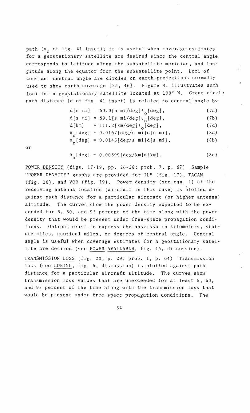
path (e0
of fig. 41 inset); it is useful when coverage estimates
for a geostationary satellite are desired since the central angle
corresponds to latitude along the subsatellite meridian, and lon
gitude along the equator from the subsatellite point. Loci of constant central angle are circles on earth projections normally
used to show earth coverage [23, 46]. Figure 41 illustrates such
loci for a geostationary satellite located at 100° W. Great-circle
path distance (d of fig. 41 inset) is related to central angle by
or
d [n mi]
d[s mi]
d[km] e [ deg]
0 8 [ deg]
0
= 60.0 [n mi/deg] 8 [deg], 0
= 69.l[s mi/deg]e0
[deg],
= 111.2[km/deg]e [deg], 0
0.0167(deg/n mi]d[n mi],
= 0.0145[deg/s mi]d(s mi],
(7a)
(7b)
(7c)
(Sa)
(8b)
80
[deg] = 0.00899[deg/km]d(km]. (8c)
POWER DENSITY (figs. 17-19, pp. 26-28; prob. 7, p. 67) Sample
"POWER DENSITY" graphs are provided for ILS (fig. 17), TACAN (fig. lS), and VOR (fig. 19). Power density (see eqn. 1) at the
receiving antenna location (aircraft in this case) is plotted a
gainst path distance for a particular aircraft (or higher antenna)
altitude. The curves show the power density expected to be ex
ceeded for 5, 50, and 95 percent of the time along with the power
density that would be present under free space propagation condi
tions. Options exist to express the abscissa in kilometers, statute miles, nautical miles, or degrees of central angle. Central
angle is useful when coverage estimates for a geostationary satel
lite are desired (see POWER AVAILABLE, fig. 16, discussion).
TRANSMISSION LOSS (fig. 20, p. 29; prob. 1, p. 64) Transmission loss (see LOBING, fig. 6, discussion) is plotted against path
distance for a particular aircraft altitude. The curves show
transmission loss values that are unexceeded for at least 5, 50, and 95 percent of the time along with the transmission loss that
would be present under free-space propagation conditions. The
54
:
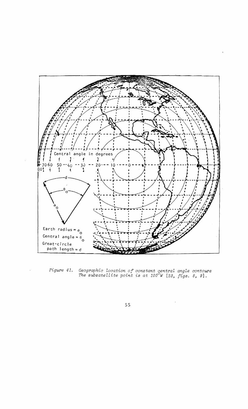
, --- .. Central angle
f 4 ; so ··4o -- 3v 1 ~ ~
Earth radius= a 0
Ce n t r a I a n g J e = e 0
Great-circle path length=d
Figure 41. Geographic location of constant central angle contours The subsatellite point is at 100°W [23~ figs. B~ 9].
55
term "GAIN" used in the parameter summary at the top of the graph
is an abbreviation for the sum of the transmitting and receiving
antennas' main beam gains. Since GAIN = 0 in this case. trans
mission loss is really basic transmission loss. Options exist
to express the abscissa in kilometers, statute miles, nautical
miles, or degrees of central angle. Central angle is useful when
coverage estimates for a geostationary satellite are desired (see
POWER AVAILABLE, fig. 16, discussion). Values obtained from figure 20 may differ somewhat from those
obtained from figure 6 since the calculations for figure 20 in
eluded lobing as part of the time variability along with horizon
effects, while those for figure 6 did not.
The increase in variability for distances somewhat less than
150 n mi (278 km) occurs because of the specular surface reflection multipath contribution to variability that occurs somewhat
inside the horizon. Lower short-term variability near the hori
zon has been observed in propagation data [1].
POWER AVAILABLE CURVES (fig. 21, p. 30; prob. 8, p. 67) Curves
of power available (see eqn. 1) at the output of the receiving
antenna are plotted against distance for several aircraft alti
tudes, a single facility antenna height, and a time availability
of 95 percent. Options exist to exnress the abscissa in kilo
meters, statute miles, or nautical miles, and to use other time
availabilities.
POWER DENSITY CURVES (fig. 22, p. 31; prob. 9, p. 68) Curves of
power density (see eqn. 1) at the receiving antenna location
(aircraft in this case) are plotted against distance for several
aircraft altitudes, a single facility antenna height, and a time
availability of 95 percent. Options exist to express the ab
scissa in kilometers, statute miles, or nautical miles, and to
use other time availabilities.
TRANSMISSION LOSS CURVES (fig. 23, p. 32; prob. 1, p. 64) Curves
of transmission loss (see LOBING, fig. 6, discussion) are plotted
56
:

against distance for several aircraft altitudes, a single facility
antenna height, and a time availability of 95 percent. Options
exist to express the abscissa in kilometers, statute miles, or
nautical miles, and to use other time availabilities.
POWER AVAILABLE VOLUME (fig. 24, p. 33; prob. 10, p. 68) Contours
for a single available power (see eqn. 1) are plotted in the alti
tude versus distance plane for time availabilities of 5, SO, and
95 percent. When symmetry about the ordinate axis can be assumed
(e.g., omnidirectional antenna), the volume formed by rotating
a contour about the ordinate axis defines the air space in which
the time availability will almost always equal or exceed that
associated with the contour used to form it. This volume might
include some air space with inadequate time availability, since
it may not describe conditions directly above the desired facility
perfectly. Noise and interference levels are not considered in
this display. Options exist to express the abscissa in kilome
ters, statute miles, or nautical miles, and to express the ordi
nate in.feet or meters.
POWER DENSITY VOLUME (fig. 25, p. 34; prob. 11, p. 68) Contours
for a single power density value are plotted in the altitude
versus distance plane for time availabilities of 5, 50, and 95
percent. When symmetry about the ordinate axis can be assumed
(e.g., omnidirectional antenna), the volume formed by rotating
a contour about the ordinate axis defines the air space in which
the time availability will almost always equal or exceed that
associated with the contour used to form it. This volume might
include some air space with inadequate time availability, since
it may not describe conditions directly above the desired facility
per ctly. Noise and interference levels are not considered in
this display. Options exist to express the abscissa in kilo
meters, statute miles or nautical miles, and to express the or
dinate in feet or meters.
TRANSMISSION LOSS VOLUME (fig. 26, p. 35; prob. 12, p. 69) Con
tours for a single transmission loss (see LOBING, fig. 6,
57
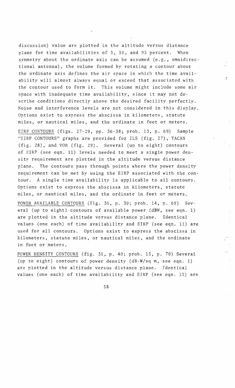
discussion) value are plotted in the altitude versus distance
plane for time availabilities of 5, 50, and 95 percent. When
symmetry about the ordinate axis can be assumed (e.g., omnidirec
tional antenna), the volume formed by rotating a contour about
the ordinate axis defines the air space in which the time avail
ability will almost always equal or exceed that associated with
the contour used to form it. This volume might include some air
space with inadequate time availability, since it may not de
scribe conditions directly above the desired facility perfectly.
Noise and interference levels are not considered in this display.
Options exist to express the abscissa in kilometers, statute
miles, or nautical miles, and the ordinate in feet or meters.
EIRP CONTOURS (figs. 27-29, pp. 36-38; prob. 13, p. 69) Sample
"EIRP CONTOURS" graphs are provided for ILS (fig. 27), TACAN
(fig. 28), and VOR (fig. 29). Several (up to eight) contours
of EIRP (see eqn. 11) levels needed to meet a single power den
sity requirement are plotted in the altitude versus distance
plane. The contours pass through points where the power density
requirement can be met by using the EIRP associated with the con
tour. A single time availability is applicable to all contours.
Options exist to express the abscissa in kilometers, statute
miles, or nautical miles, and the ordinate in feet or meters.
POWER AVAILABLE CONTOURS (fig. 30, p. 39; prob. 14, p. 69) Sev
eral (up to eight) contours of available power (dBW, see eqn. 1)
are plotted in the altitude versus distance plane. Identical
values (one each) of time availability and EIRP (see eqn. 11) are
used for all contours. Options exist to express the abscissa in
kilometers, statute miles, or nautical miles, and the ordinate
in feet or meters.
POWER DENSITY CONTOURS (fig. 31, p. 40; prob. 15, p. 70) Several
(up to eight) contours of power density (dB-W/sq m, see eqn. 1)
are plotted in the altitude versus distance plane. Identical
values (one each) of time availability and EIRP (see eqn. 11) are
58
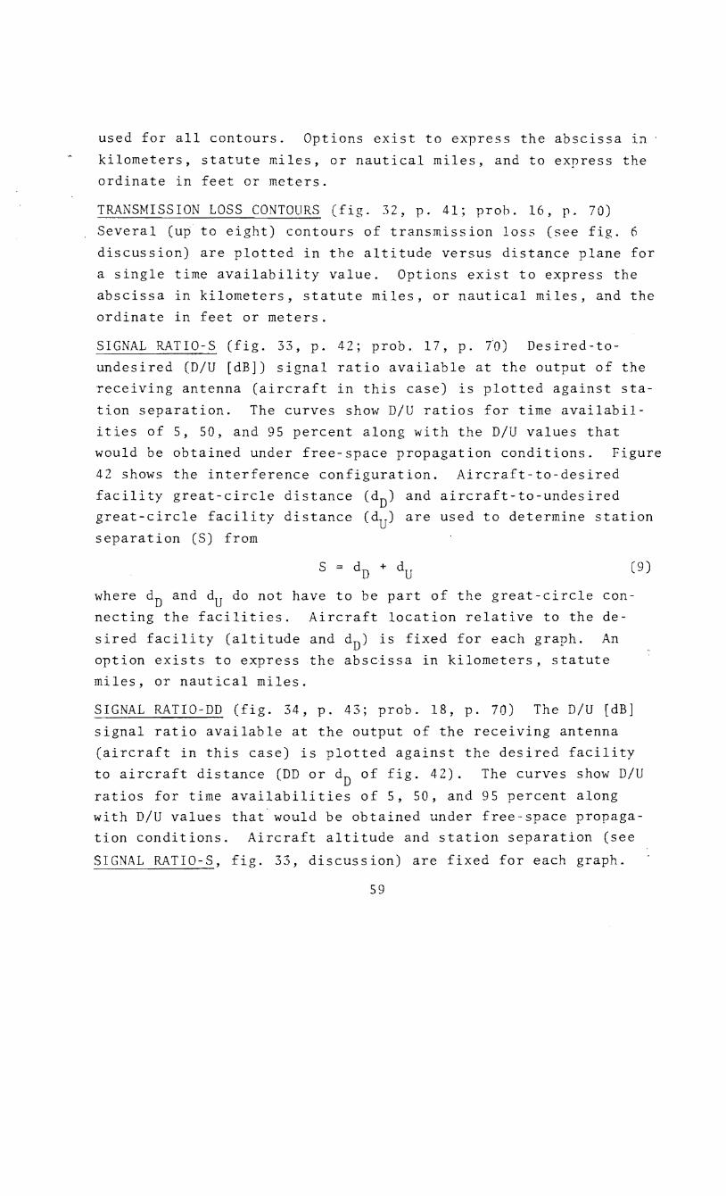
used for all contours. Options exist to express the abscissa in
kilometers, statute miles, or nautical miles, and to express the
ordinate in feet or meters.
TRANSMISSION LOSS CONTOURS (fig. 32, p. 41; prob. 16, p. 70)
Several (up to eight) contours of transmission loss (see fig. 6
discussion) are plotted in the altitude versus distance plane for
a single time availability value. Options exist to express the
abscissa in kilometers, statute miles, or nautical miles, and the
ordinate in feet or meters.
SIGNAL RATIO-S ( g. 33, p. 42; prob. 17, p. 70) Desired-to
undesired (D/U [dB]) signal ratio available at the output of the
receiving antenna (aircraft in this case) is plotted against sta
tion separation. The curves show D/U ratios for time availabil
ities of 5, SO, and 95 percent along with the D/U values that
would be obtained under free space propagation conditions. Figure
42 shows the inter renee configuration. Aircraft-to-desired
facility great-circle distance (dD) and aircraft-to-undesired
great-circle facility distance (du) are used to determine station
separation (S) from
s
where dD and du do not have to be part of the great-circle con
necting the facilities. Aircraft location relative to the de
sired facility (altitude and dD) is xed for each graph. An
option exists to express the abscissa in kilometers, statute
miles, or nautical miles.
(9)
IGNAL RATIO-DD (fig. 34, p. 43; prob. 18, p. 70) The D/U [dB]
signal ratio available at the output of the receiving antenna
(aircraft in this case) is plotted against the desired facility
to aircra distance (DD or dD of fig. 42). The curves show D/U
ratios for time availabilities of 5, SO, and 95 percent along with D/U values that would be obtained under free-space propagation conditions. Aircraft altitude and station separation (see
SIG~AL RATIO-S, fig. 33, discussion) are fixed for each graph.
59
0 Vl
'"C VI It .....
U1 U1
60
An option exists to express the abscissa in kilometers, statute
miles, or nautical miles. ..
ORIENTATION (fig. 35, p. 44; prob. 19, p. 71) Curves showing the
relative azimuthal orientation of the undesired facility course
line C~u) with respect to the great circle-path connecting the
desired and undesired facilities are plotted versus the facility
separation required to achieve a specified D/U ratio or better at
each of five specified protection points. Each curve represents
a different relative azimuthal orientation of the desired facility
course line (¢D) with respect to the path connecting facilities.
Orientation geometry for the protection points is illustrated in
figure 43. These protection points are located relative to the
desired facility by a distance from the desired (D ) A,B,C,D,E facility and relative azimuth angle from the desired facility
course line (aA BCD E). In the calculations for figure 35, (a) ' ' ' ' the protection points were at
Distance Angle
DA = 10 n mi (18. 5 km) a A = 32 5°
DB 18 n mi (33.3 km) aB 350°
DC = 18 n mi (33.3 km) ac = oo DD = 18 n mi (33.3 km) aD = 10°
DE = 10 n mi (18. 5 km) aE = 35°
(b) ~D was varied in 30° increments from 0 to 180° (see line code
in upper right of fig. 35), (c) ~U was varied in 10° increments
from 0 to 360°, and (d) azimuth (horizontal) patterns for the
8-loop localizer were used for both facilities.
Protection point C on figure 43 is used to illustrate the
difference between facility separation (Sf) calculated via pro
gram TWIRL and station separation (S) used elsewhere (see SIGNAL
RATIQ-~, fig. 33, discussion). In particular, Sf~ S since S
need not be measured along the great-circle path connecting the
facilities. Note that (a) the du to point C changes as.~D changes, even if Sf remains fixed, and (b) the angle from the
61
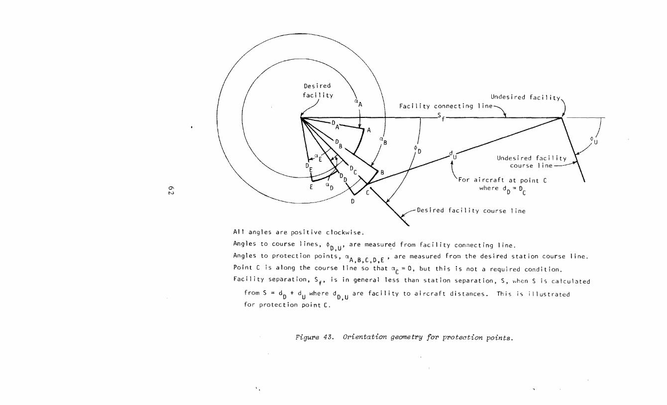
Q'\ N
Desired facility
Facility connecting Undesired
ir==::::: ~ I I I s f .
All angles are positive clockwise.
du
\For Undesired facility
course line
aircraft at point C where d
0 =DC
Desired facility course line
Angles to course lines, *o,u• are measured from facility connecting line.
Angles to protection points, a E, are measured from the desired station course line. A,B,C,D,
Point C is along the course line so that aC = 0, but this is not a required condition.
Facility separation, Sf' is in general less than station separation, S, ~henS is calculated
from S = d0 + dU where d0 U are facility to aircraft distances. This is illustrated •
for protection point C.
Figure 43. Orientation geometry for protection points.

undesired facility to point C chan s with both ¢0 and ¢u even if
Sf remains fixed, so that the applicable gain for the undesired
facility varies in accordance with its horizontal pattern.
The geometrical consequences of these complications are
handled as part of the calculations performed by program TWIRL.
These calculations would be very tedious to perform by hand even
if appropriate signal ratio graphs (fig. 33) were available. A
graph similar to figure 35 is constructed for each protection
point and the maximum Sf for each combination of ¢0 and ¢u is
selected for the final graph. These intermediate graphs have a
format identical to figure 35 and are available as computer out-·
put even though no samples are provided here.
Options exist to express the abscissa in kilometers, statute
miles, or nautical miles.
§ERVICE VOLUME (figs. 36-37, p. 45-46; prob. 20, p, 71) Sample "SERVICE VOLUME" graphs are provided for TACAN (fig. 36) and
VOR (fig. 37). Fixed D/U contours are plotted in the altitude
versus distance plane for free space conditions and for time
availabilities of 5, SO, and 95 percent. A fixed station separa
tion (see SIGNAL RATIO-S, fig. 33, discussion) is used for each
graph. When symmetry about the ordinate axis can be assumed
(e.g., omnidirectional antenna), the volume formed by rotating
a contour about the ordinate axis defines the air space in which
the time availability will almost always equal or exceed that
associated with the contour used to form it. This volume might
include some air space with inadequate time availability, since
it may not describe conditions directly above the desired facil
ity perfectly. Service limitations associated with noise level
are not considered in this display. Options exist to express the
abscissa in kilometers, statute miles, or nautical miles, and the
ordinate in et or meters.
SIGNAL RATIO CONTOURS (figs. 38-39, pp. 47-48; prob. 21, p. 71)
Sample "SIGNAL RATIO CONTOURS" graphs are provided for ILS (fig.
38) and VOR (fig. 39). Several (up to eight) D/U signal ratio
63

contours are plotted in the altitude versus distance plane (cf.,
figs. 36, 37). Single values of time availability and station separation are used for each graph. Options exist to express the
abscissa in kilometers, statute miles, or nautical miles, and the
ordinate in feet or meters.
3.3 APPLICATIONS Graphs like those provided in section 3.1 and discussed in
section 3.2 can be used to solve a wide variety of problems where
system reliability is dependent upon radio-wave propagation. The
application of each plotting capability is illustrated by a prob
lem and solution in the remainder of this section. These prob
lems are ordered by the capability applied in accordance with the
table 1 listing.
LOBING GRAPH (fig. 1, p. 10; fig. 6, p. lS; fig. 20, p. 29; fig.
23, p. 32).
Problem 1: Estimate the extent of smooth earth coverage for a
system with the parameters of figure 1 and an allowable transmis
sion loss of 13S dB.
Solution: Figure 6 indicates potential coverage gaps from
7S to 87 n mi (139 to 161 km) and no coverage beyond 232 n mi
(430 km). Figure 20 indicates coverage to 2S9, 233, and 220 n mi
(480, 432, and 407 km) for time availabilities of S, SO, and 9S
percent. Figure 20 has the effects of surface reflection multi
path included statistically in the signal level variability so
that nulls, while not ~hown, are accounted for in the time availability estimate. Figure 20 also provides a better estimate of
transmission loss near the horizon. Figure 23 could have been
used instead of figure 20 to obtain coverage for a 9S percent time availability.
REFLECTION COEFFICIENT (fig. 6, p. is; fig. 7, p. 16; fig. 12, p.
21; fig. 13, p. 22; fig. 14, p. 23). Problem 2: Determine the reflection coefficient, reflection
64
.-
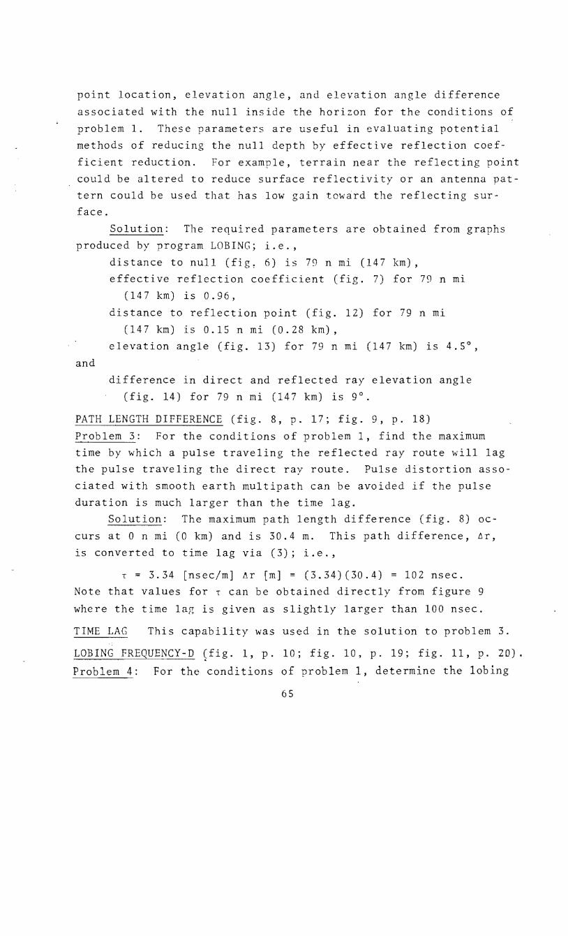
point location, elevation angle, and elevation angle fference
associated with the null ide the horizon for the conditions of
problem 1. These parameters are useful in evaluating potential
methods of reducing the null depth by effective reflection coef
ficient reduction. For example, terrain near the reflecting point
could be altered to reduce surface reflectivity or an antenna pat
tern could be used that has low gain tow~rd the reflecting sur
face.
Solution: The required parameters are obtained from graphs
produced by program LOBING; i.e.,
and
distance to null (fig~ 6) is 79 n mi (147 km),
effective reflection coe cient (fig. 7) for 79 n mi
(147 km) is 0.96,
distance to reflection point (fig. 12) for 79 n mi
(147 km) is 0.15 n mi (0.28 km),
elevation angle (fig. 13) for 79 n mi (147 km) is 4.5°,
difference in direct and reflected ray elevation angle
(fig. 14) for 79 n mi (147 km) is 9°.
PATH LENGTH DIFFERENCE (fig. 8, p. 17; fig. 9, p. 18)
Problem 3: For the conditions of problem 1, find the maximum
time by which a pulse traveling the reflected ray route will lag
the pulse traveling the direct ray route. Pulse distortion asso
ciated with smooth earth multipath can be avoided if the pulse
duration is much lar r than the time lag.
Solution: The maximum path length difference (fig. 8) oc
curs at 0 n mi (0 km) and is 30.4 m. This path difference, ar,
is converted to time lag via (3); i.e.,
-r = 3.34 [nsec/m] t.r [m] = (3.34)(30.4) = 102 nsec.
Note that values for -r can be obtained directly from gure 9
where the time lag is given as slightly larger than 100 nsec.
TIME LAG This capability was used in the solution to problem 3.
LOBING -D (fig. 1, p. 10; fig. 10, p. 19; g. 11, p. 20).
Problem 4: For the conditions of problem 1, determine the lobing
65
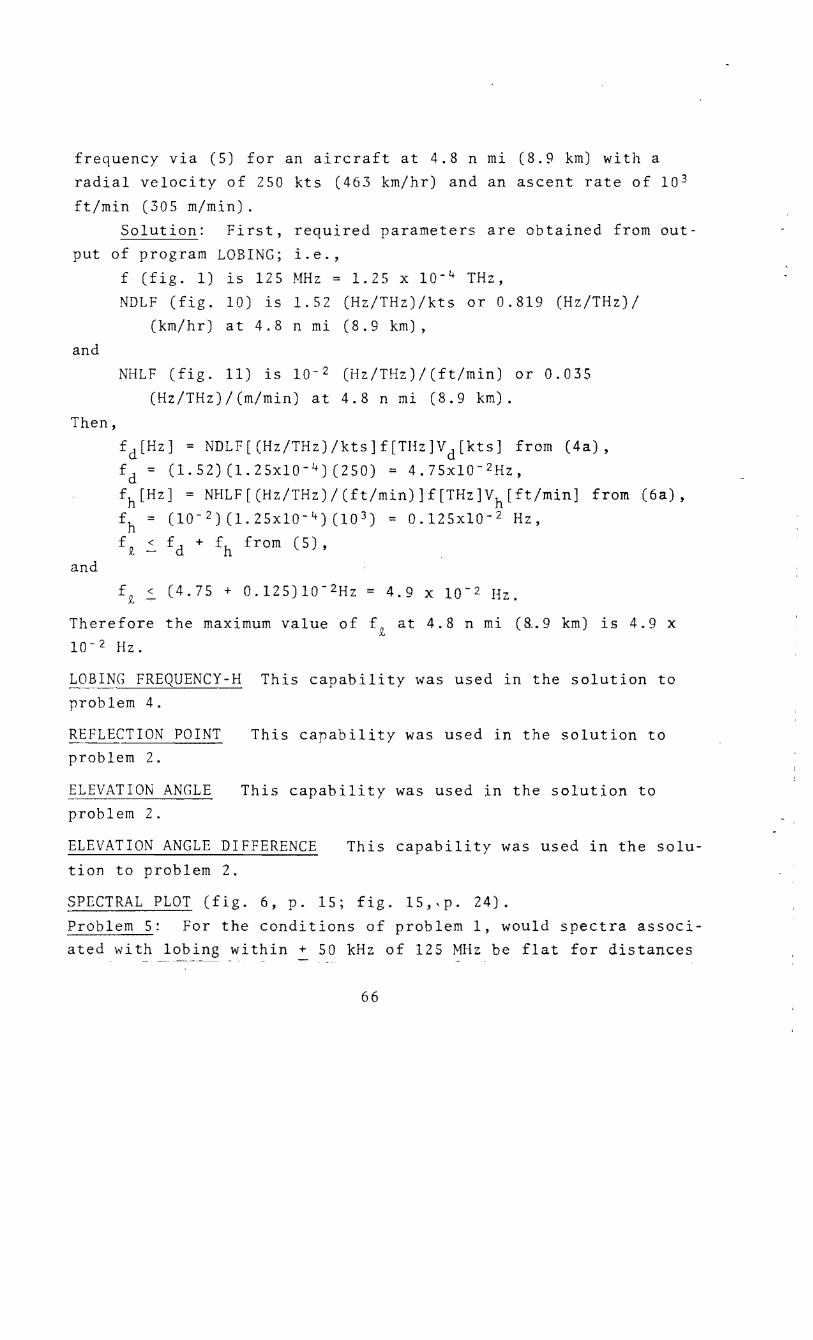
frequency via (5) for an aircraft at 4.8 n mi (8.9 km) with a radial velocity of 250 kts (463 km/hr) and an ascent rate of 10 3
ft/min (305 m/min). Solution: First, required parameters are obtained from
put of program LOBING; i . e. ,
and
Then,
f (fig. 1) is 125 MHz = 1. 25 X 10- 4 THz,
NDLF (fig. 10) is 1. 52 (Hz/THz)/kts or 0.819 (Hz/THz)/ (km/hr) at 4.8 n mi (8.9 km),
NHLF (fig. 11) is 10-2 (Hz/THz)/(ft/min) or 0.035
(Hz/THz)/(m/min) at 4.8 n mi (8.9 km).
fd[Hz] = NDLF[(Hz/THz)/kts]f[THz]Vd[kts] from (4a), fd = (1.52)(1.25xlo-4)(250) = 4.75xlo-2Hz,
out-
fh[Hz] = NHLF[(Hz/THz)/(ft/min)]f[THz]Vh[ft/min] from (6a), fh (lo- 2) (1.25xlQ-4) (103) = 0.125xlo- 2 Hz,
f1
< fd + fh from (5), and
f1
< (4.75 + 0.125)10- 2 Hz = 4.9 x lo-z Hz.
Therefore the maximum value of f1
at 4.8 n mi (&.9 km) is 4.9 x lo- 2 Hz.
L~~ING FREQUENCY-H This capability was used in the solution to problem 4.
REFLECTION POINT problem 2.
This capability was used in the solution to
ELEVATION ANGLE
problem 2. This capability was used in the solution to
ELEVATION ANGLE DIFFERENCE
tion to problem 2. This capability was used in the solu-
SPECTRAL PLOT (fig. 6, p. 15; fig. 15,,p. 24).
Problem 5: For the conditions of problem 1, would spectra associated with lobing within + 50 kHz of 125 MHz be flat for distances
66

from 27 n mi (50 m) to the radio horizon? Frequency selective
fading (i.e., when all frequencies within a receiver bandpass do•
not fade together) can distort a modulated signal so that intel
ligibility is lowered. It does not occur when spectra are flat.
Solution: Figure 6 indicates that the top of the lobe 4 oc
curs at a distance somewhat less than 27 n mi (50 km). Therefore,
the spectra shown in figure 15 are applicable to this problem,
and these spectra are flat, so the answer is yes.
POWER AVAILABLE, UHF SATELLI (fig. 3, p. 12; fig. 16, p. 25).
Problem 6: Determine how far north coverage from a geostationary
UHF satellite extends when the parameters of figure 3 are appli
cable, and a time availability of 95 percent and a power available
of -160 dBW are required.
Solution: Figure 16 is applicable to this problem, and it
indicates that coverage out to an angular distance of 80° can be
obtained for the required time availability. Therefore, coverage
to 80°N is possible along the subsatellite meridian. The great
circle distance for this arc can be obtained using (7c); i.e.,
d[km] = 111.2 [km/deg]e0
[deg],
(111.2)(80) ~ 8,900 km (4,800 n mi).
POWER DENSITY (fig. 5, p. 14; fig. 19, p. 28)
Problem 7: For the VOR parameters of figure 5, determine the in
terference range of a VOR at 30,000 ft (9,144 m) when a time a
vailability of 5 percent and a power density of -134 dB-W/sq m
or more are used to define the interference range.
Solution: Figure 19 is applicable to this problem, and it
indicates an interference range of 236 n mi (437 km).
TRANSMISSION LOSS
problem 1.
This capability was used in the solution to
POWER AVAILABLE CURVES (fig. 1, p. 10; fig. 21, p. 30)
Problem 8: For the ATC parameters of figure 1 where the aircraft
is at 45,000 ft (13,716 m), determine the service range when a
67
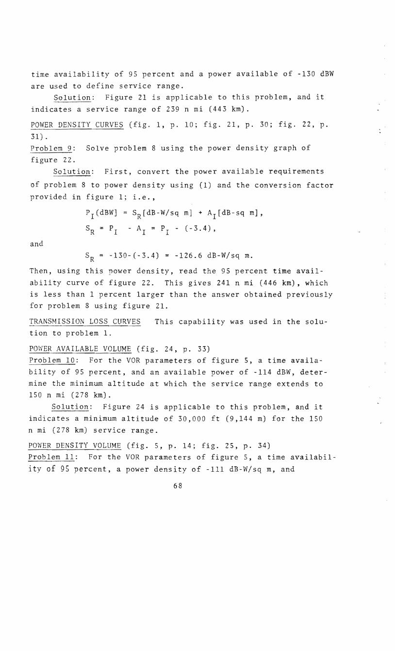
time availability of 95 percent and a power available of -130 dBW
are used to define service range. Solution: Figure 21 is applicable to this problem, and it
indicates a service range of 239 n mi (443 km).
POWER DENSITY CURVES (fig. 1, p. 10; fig. 21, p. 30; fig. 22, p.
31). Problem 9: Solve problem 8 using the power density graph of
figure 22. Solution: First, convert the power available requirements
of problem 8 to power density using (1) and the conversion factor
provided in figure 1; i.e.,
and
P1 (dBW] = SR[dB-W/sq m] + AI[dB sq m],
SR = PI - AI = PI - (-3.4),
SR = -130-(-3.4) = -126.6 dB-W/sq m.
Then, using this power density, read the 95 percent time avail
ability curve of figure 22. This gives 241 n mi (446 km), which
is less than 1 percent larger than the answer obtained previously for problem 8 using figure 21.
TRANSMISSION LOSS CURVES
tion to problem 1. This capability was used in the solu-
POWER AVAILABLE VOLUME (fig. 24, p. 33) Problem 10: For the VOR parameters of figure 5, a time availa
bility of 95 percent, and an available newer of -114 dBW, deter
mine the minimum altitude at which the service range extends to 150 n mi (278 km).
Solution: Figure 24 is applicable to this problem, and it
indicates a minimum altitude of 30,000 ft (9,144 m) for the 150
n mi (278 km) service range.
POWER DENSITY VOLUME (fig. 5, p. 14; fig. 25, p. 34)
Problem 11: For the VOR parameters of figure 5, a time availabil
ity of 95 percent, a power density of -111 dB-W/sq m, and
68
altitudes up to 100,000 ft (30,480 m), determine aircra
for which service is not available at 150 n mi (278 km).
altitudes
Solution: Figure 25 is applicable to this problem, and it
indicates that service is not available at 150 n mi (278 km) for
altitudes below 31,000 (9,449 m).
TRANSMISSION LOSS VOLU!v1E (fig. 5, p. 14; fig. 26, p. 35)
Problem 12: For the VOR parameters of figure 5, a time availa
bility of 50 percent, and altitudes up to 100,000 ft (30,480 m),
determine the altitudes for which a basic transmission loss of
134 dB is exceeded at a distance of 175 n mi (324 km).
Solution: Figure 26 is applicable, and it indicates that
the 134 dB transmission loss level is exceeded 50 percent of the
time at a distance of 175 n mi (324 km) for altitudes below
40,000 ft (12,192 m).
EIRP CONTOURS (fig. 4, p. 13; fig. 28, p. 37)
Problem 13: For the TACAN parameters of figure 4, determine the
minimum EIRP of transmitted pulses necessary to maintain a pulse
power density greater than -86 dB-W/sq m for 95 percent of the
time at an altitude of 30,000 ft (9,144 m) and a distance of
125 n mi (232 km).
Solution: Figure 28 is applicable to this problem, and it
indicates that an EIRP of 42 dBW would be sufficient.
POWER AVAILABLE (fig. 4, p. 13; fig. 30, p. 39)
Problem 14: For the TACAN parameters of figure 4, a service range
defined by a time availability of 95 percent, and a power density
of -86 dB-W.sq m, determine the service range available at 30,000
ft (9,144 m) by using figure 30.
Solution: First convert the power density requirement to
power available using (1) and the conversion factor provided in
figure 4 ; i . e . ,
and
PI[dBW] = Sa[dB-W/sq m] + AI[dB-sq m],
PI = -86+( 22.7) = -108.7 dBW.
Then, using this power available, read the 95 percent time
69
availability curve of figure 30. This gives 111 n mi (206 km).
POWER DENSITY CONTOURS (fig. 4, p. 13; fig. 30, p. 39; fig. 31,
p. 40).
Problem 15: Solve problem 14 using figure 31.
Solution: Figure 31 indicates that the service range at
30,000 ft (9,144 m) is 111 n mi (206 km), which is the same an
swer obtained previously for problem 14 usine figure 30.
TRANSMISSION LOSS CONTOURS (fig. 4, p. 13; fig. 32, p. 41)
Problem 16: For the TACAN parameters of figure 4 and a time a
vailability of 95 percent, determine the minimum altitude for
which a basic transmission loss of 150 dB is not exceeded at a
distance of 100 n mi (185 km).
Solution: Figure 32 is applicable since it was developed
with antenna gains set to zero so that basic transmission loss
is obtained. It indicates that 150 dB of basic transmission loss
is not exceeded for 95 percent of the time at 100 n mi (185 km)
for altitudes above 18,000 ft (5,486 m).
SIGNAL RATIO-S (fig. 5, p. 14; fig. 33, p. 42; fig. 42, P• 60) Problem 17: For the VOR parameters of figure 5, a time availa
bility of 95 percent, and a desired facility to aircraft distance,
dD' of 100 n mi (185 km), determine the station separation (fig. 42) necessary to obtain a desired-to-undesired signal ratio, D/U,
of 23 dB at an altitude of 30,000 ft (9,144 m).
Solution: Figure 33 is applicable to this problem, and it indicates that a station separation of 320 n mi (593 km) is ade
quate to obtain D/U (95%) = 23 dB with dD = 100 n mi (185 km).
However, this signal ratio is not available beyond 100 n mi
(185 km) for altitudes less than 30,000 ft (9,144 m).
SIGNAL RATIO-DD (fig. 5, p. 14; fig. 34, p. 43)
Problem 18: For the VOR parameters of figure 5, a time availa
bility of 95 percent, and a D/U of 23 dB or more, determine the maximum dD available for a station separation of 250 n mi (463
km).
70
Solution: Figure 34 is applicable to this problem and it
indicates that a maximum dD of 59 n mi (109 km) is available.
!ENTATION ( g. 2, p. 11; fig. 35, p. 44; fig. 43, p. 62)
Problem 19: For the ILS localizer parameters of figure 2, but
with altitude of 4500 ft (1,372 m), the protection point loca
tions associated with figure 43 (see ORIENTATION, fig. 35, dis
cussion in sec. 3.2), a time availability of 95 nercent, and a
D/U of 23 dB determine the facility separation required when the
undesired course line angle (¢u in fig. 43) is 150° and the de
sired course line angle (¢D of fig. 43) is 60°.
Solution: Figure 35 is applicable to this problem, and it
indicates that a facility separation of 88 n mi (163 km) is suf
cient.
SERVICE VOLUME (fig. 5, p. 14; fig. 37, p. 46)
Problem 20: For the VOR parameters of figure 5, a time availa
bility of 95 percent, and a station separation of 400 n mi (741
km), determine the maximum dD for which D/U = 23 dB is available
at an altitude of 40,000 ft (12,192 m).
Solution: Figure 37 is applicable to this problem, and it
indicates that a dD of 144 n mi (267 km) is available at 40,000
ft ( 12, 19 2 m) .
SIGNAL RATIO CONTOURS (fig. 2, p. 11; fig. 38, p. 47)
Problem 21: For the ILS localizer parameters of figure 2, a time
availability of 95 percent, and a station separation of 95 n mi
(176 km), determine the maximum dD available at 1,000 ft (305m)
for which D/U ~ 23 dB.
Solution: Figure 38 is applicable to this problem, and it
indicates that a dD of 30 n mi (56 km) is available at 1,000 ft
(305 m) .
4. INPUT PARM1ITERS
Parameters that may be specified as input to the programs
are summarized in tables 2, 3, and 4. Blank spaces are provided
71

in these tables so that copies of them can be used to specify in
put requirements for program runs. These tables cover input para
meters for 10 programs which have 28 plotting capabilities (table 1) so that only information for a small f~action of the parameters
listed need be provided for any one capability.
Table 2 covers general parameters that are usually a~plicable to many programs, and multiple entries or two copies of this table
may be used if the desired and undesired facilities have different
parameter values. Note that, although about 40 items can he spe
cified, specification of only 3 is required. These "primary pa
rameters" consist of antenna heights and frequency. Values for
"secondary parameters" will be computed or assumed if not speci
fied. A more detailed discussion of table 2 is provided in sec
tion 4.1.
Table 3 covers special parameters required for particular
capabilities. Some of these parameters are required by more than
one capability, and 13 (i.e., first 13 of table 1) of the capa
bilities do not require parameters from table 3. Additional dis
cussion of table 3 is provided in section 4.2.
Table 4 covers parameters associated with graph formats. In
many cases, an adequate selection of these·parameters can be made
by the program operator so that complete speci cation via table
4 is not often required. Options associated with ordinate (feet
or meters) and/or abscissa (kilometers, statute miles, or nau
tical miles) units are available. These options are selected via
table 4. A more detailed discussion of table 4 is provided in
section 4.3.
4.1 GENERAL PARAMETERS (Table 2, p. 73)
General parameters that are usually applicable to many pro
grams may be specified by using copies of table 2. Multiple en
tries or two copies of this table may be used·if the desired and
undesired facilities have different parameter values associated with them. In the absence of such information, it will be as
sumed that the two facilities have identical parameters. All
72
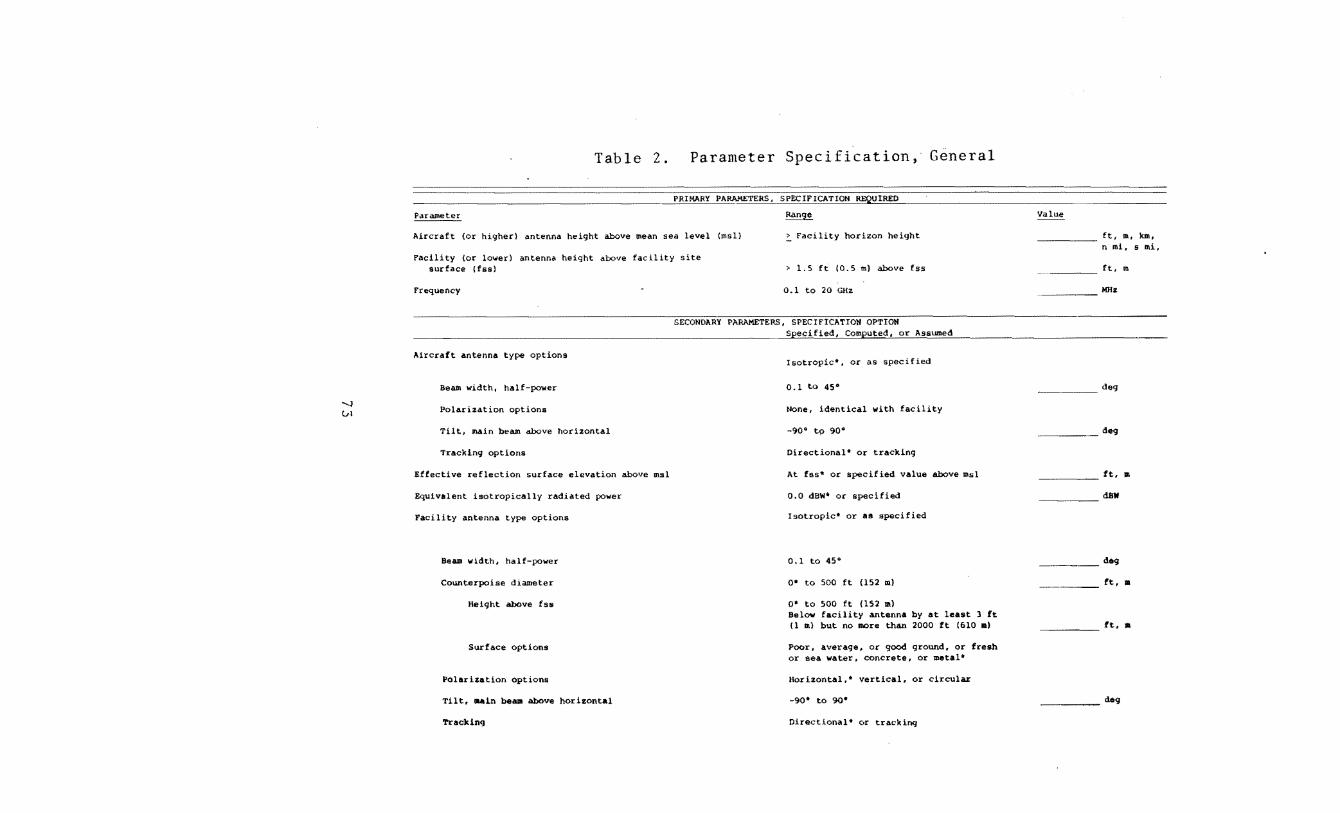
'-J vt
Table 2. Parameter Specification, General
--------------------------------------------~P~R~IMA~R~Y~P~A~RAMETERS, SPECIFICATION REQUIRED
Parameter
Aircraft (or higher) antenna height above mean sea level (msl)
Facility (or lower) antenna height above facility site surface (fss)
Frequency
Range
~ Facility horizon height
> 1.5 ft (0.5 m) above fss
0.1 to 20 GHz
SECONDARY PARAMETERS, SPECIFICATION OPTION Specified, Computed, or Assumed
Aircraft antenna type options
Beam width, half-power
Polarization options
Tilt, main beam above horizontal
Tracking options
Effective reflection surface elevation above msl
Equivalent isotropically radiated power
Facility antenna type options
Beam width, half-power
Counterpoise diameter
Height above fss
Surface options
Polarization options
Tilt, ~in beam above horizontal
Tracking
Isotropic*, or as specified
0.1 to 45°
None, identical with facility
-9o• t 9 go•
Directional* or tracking
At fss• or specified value above msl
0.0 dBW* or specified
Isotropic• or as specified
0.1 to 45•
o• to 500 ft (152 ml
o• to 500 ft (152 ml Below facility antenna by at least 3 ft (1 m) but no more than 2000 ft (610 a)
Poor, average, or good ground, or fresh or sea water, concrete, or metal*
Horizontal,* vertical, or circular
-90" to 90•
Directional* C•r trackinq
Value
ft, m, k.nt, n mi, s tni,
ft, m
MHZ
deg
d0!9
ft, Ill
_____ dllll
-·-- deg
f't, •
ft, •
deg

-...]
.f;>.
Table 2.
Frequency fraction (half-bandwidth)
Gain, receiving antenna (main beam}
Transmitting antenna (main beaJII)
Transmitting antenna location
Horizon obstacle distance from facility
Parameter Specification, General (cont.)
Ran9e
0 to 0.2 {0.1)*
o• to 60 dBi
o• to 60 dBi
Aircraft or facility*
From 0.1 to l times smooth earth horizon distance (calculated)*
Elevation angle above horizontal at facility <12 deg (calculated)*
Height above msl
Ionospheric scintillation options
Frequency scaling factor
Index group
Rain attenuation options
Attenuation/km
Storm si:te
ZOne
Refractivity
Effective earth's radius
or ainimum monthly mean, N0
Surface reflection lobing options
0* to 15,000 ft-msl(4572 m-msl) and ~ aircraft altitude
No scintillation* or specified
Not used* or (136/frequency in Mllz)n with l<n< 2
0* to 5, 6 for variable
NOne* or c0111puted with dB/km or zone
0 dB/km and up
5, 10,* 20 laa
l t:o 6
4010 to 6070 n mi (74l7 to 11,242 kal
200 to 400 N-units (301 N-units)*
Contributes to variability* or determines ...,dian level
~
___ ___;dBi
____ dlli
ra.un ai, ----__ __:de9
ft, •
___ ...::dB/ka
lr-ii II ai. -----'
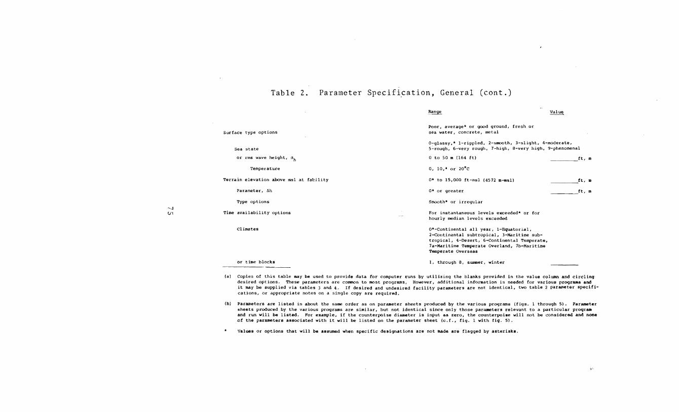
~-J
U1
Table 2. Parameter Specifi~ation, General (cont.)
Surface type options
Sea state
or rms wave height, crh
Temperature
Terrain elevation above msl at fa~ility
Parameter, ~h
Type options
Time availability options
Climates
or time blocks ---------
Range
Poor, average• or good ground, fresh or sea water 1 concrete, metal
Value
O~glassy,* 1-rippled, 2-smooth, 3-slight, 4-moderate, 5-rough, 6-very rough, 7-high, a-very high, 9-pt,enomenal
0 to 50 m (164 ft)
0, 10,. or 2:0°C
o• to 15,000 ft-msl (4572 m-m$1)
o• or greater
Smooth* or irregular
For instantaneous levels exceeded* or for hourly median levels exceeded
o•-continental all year, 1-Equatorial, 2-Q:>ntinental subtropical, 3-Marlt ime subtropical, 4-Desert,-6-continental Temperate, ?a-Maritime Temperate Overland, 7b-Maritime Temperate Overseas
1, through 8, summer, winter
_____ ft, m
_____ ft, 1D
ft, m
(a) Copies of this table may be used to provide data for computer runs by utilizing the blanks provided in the value column and circling desired options. These parameters are common to most programs, However, additional information is needed for various programs and it may be supplied via tables J and 4. If desired and undesired facility parameters are not identical, two table 2 parameter specifications, or appropriate notes on a single copy are required.
(b) Parameters are listed in about the same order as on parameter sheets produced by the various programs (figs. 1 through 5). Parameter sheets produced by the various programs are similar, but not identical since only those parameters relevant to a particular proqra. and run will be listed. For example, if the counterpoise diameter is input as zero, the counterpoise will not be considered and none nf the parameters associated with it will be listed on the parameter sheet (c.f., fig. l with fig. 5).
Values or options that will be asaumed when specific designations are not made are flagged by asterisks.
!.' ~
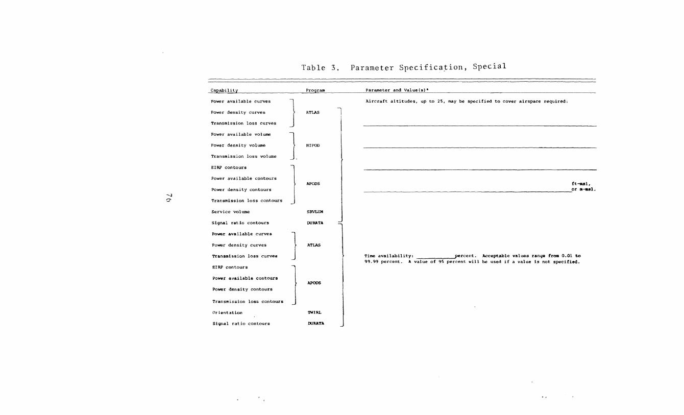
'-l 0
Table 3.
Capability Program
Power available curves
Power density curves
Transmission loss curves
Power available volume
Power density volume
Transmission loss volume
EIR.P contours
Power available contours
Power density contours
Transmission loss contours
Service volume
Signal ratio contours
Power available curves
Power density curves
Transmlssi~n loss curves
EIR.P contours
Power available contours
Power density contours
Transmission loss contour$
Or!ent.1tion
Si~\al ratio contours
} J l }
J
ATLAS l
HI POD
APODS
SRVWM
OURATA
ATLAS
APOOS
TWIRL
DURATA
Parameter Specification, Special
Parameter and Value(s)•
Aircraft altitudes, up to 25, may be sp&cified to cover airspace required:
ft-mal,
--------------------------------------------------------------------~or m-sal.
Time availability: percent. Acceptable values ran~• from 0.01 to 99.99 percent. A value of 95 percent will be used if a value ls not specified.
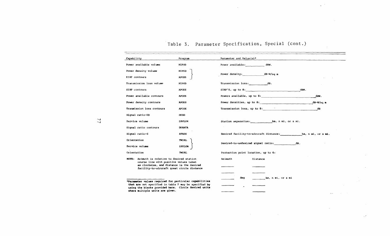
"-1 "-1
Table 3. Parameter Specification, Special (cont.)
Caj2abilit~ Pr~ram
Power available volume HI POD
Power density volume HI POD J EIRP contours APODS
Transmission loss vol~ HI POD
I!IR:P contours APOOS
Power available contours APOOS
Power density contours APOOS
Tra~ission loss contours J\1'005
Signal ratio-DO 0000
Service 110lume SRVUIM
Signal ratio contours DURATA
Signal ratio-S ATJ\DU
Orientation TWIRL }
Service volume SRV'LUM
Orientation TWIRL
NOTE: Azimuth is relative to desired station course line with positive values taken as clockwise, and distance is the desired facility-to-aircraft great circle distance
*Par~r valuea required for particular capabilities that are not specified in table 2 may be specified by using the blanks provided here. Circle desired unite Where aultiple units are given.
Parameter and Value(s)•
Power available: dBW.
Power density:~ __ _dB-W/sq m
Transmission loss: dB.
EIRP'S, up to 8: dBW.
Powers available, up to 8: dBW.
Power densities, up to 8: dB-W/sq m
Transmission loss, up to 8: dB
Station separation: km, n mi, or s mi.
Desired facility-to-aircraft distance: km, n mi, or s mi.
Desired-to-undesired signal ratio: dB.
Protection point location, up to 6:
Azimuth Distance
deg ____ k.m# n mif or s mi
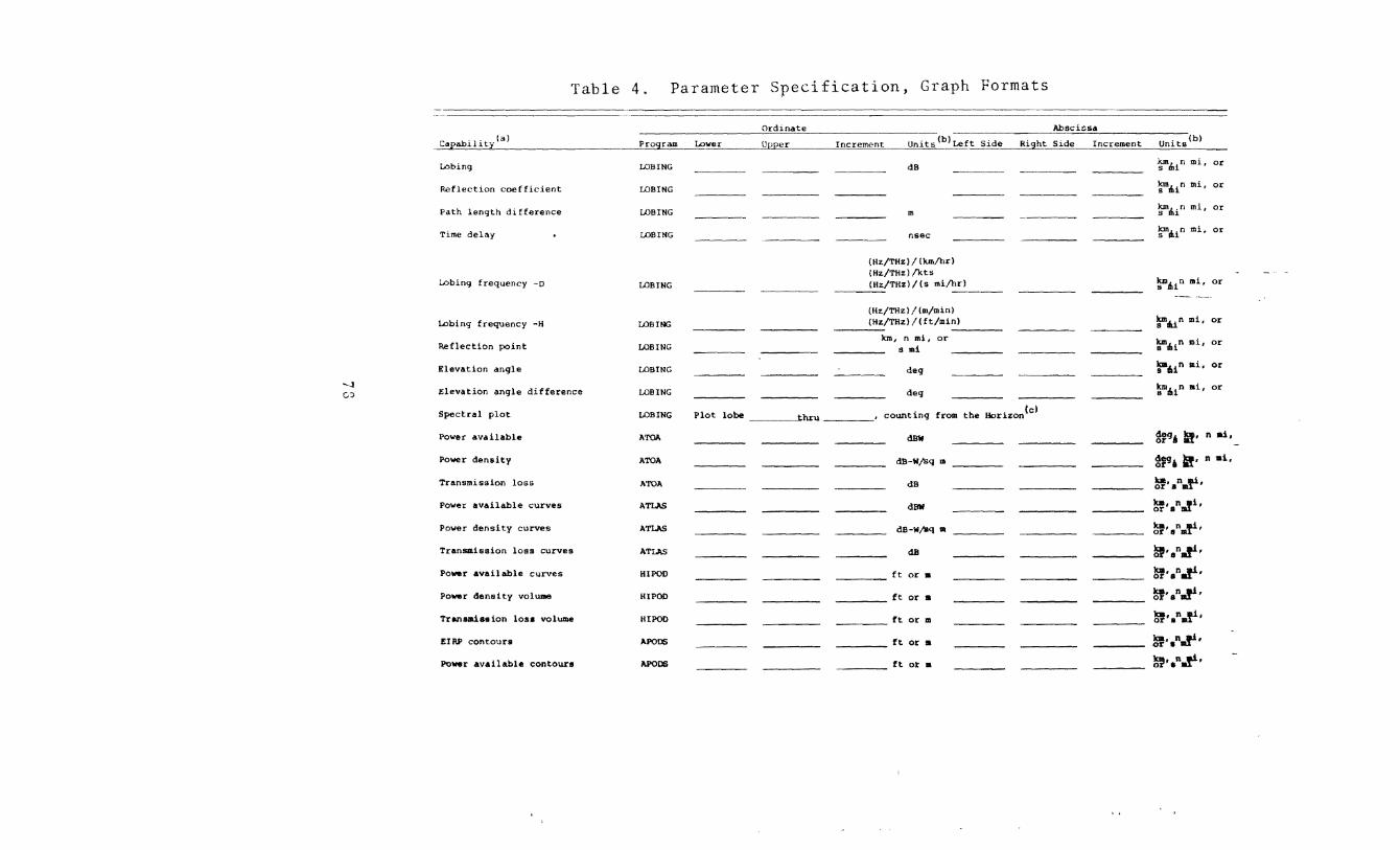
'"--! c::>
Table 4. Parameter Specification, Graph Formats
Capability(a) __ ~~og~am Lower
Lobinq LOSING
Reflection coefficient LOSING
Path length difference LOSING
Time delay LOSING
Lobing frequency -D LOSING
Lobing frequency -H LOB!NG
Reflection point LOSING
Elevation angle t..OBING
Elevation angle difference LOSING
Spectral plot LOSING Plot lobe
Power available ATOA
Power density ATOA
Transmission loss ATOA
Power available curves ATLAS
Power density curves ATLAS
Transmission loss curves ATI.AS
Powr available curves HI POD
Power density volume Ill POD
Transmia•ion losa volume lliPOD
EIRP contours APODS
Power available contours APODS
Ordinate
Upper Il'lcremenL Unit:_.;_ (b) Left Side Right
dB
m
nsec
(llz/THz)/(lon/hr) (Hz/THz) /kts
--~~ll~z=/Tllz) I (s mi!h_r_> __ _
(Hz/THzl/lm/min) _____ l_Hz_/THz)/!ft/mi_n_l ____ __
Jan, n mi, or s mi
deg
deg
--------~hru , counting from the Horizon(c)
dBW
dB-W/Sq m
dB
dBif
dB-W/11q Ill
dB
ft or •
ft or •
ft or 111
ft or •
ft or •
Absci.csa
~zld" mi, or
l?'n.t n mi, or
~thin mi, or
~dlin mi, or
l?'dlt n mi, or
l?'.tun mi, or
ll"'z~.t" mi, or
ll:'-~ot" mi, or
l?'.t.in ai, or
~gil lf• n ai,
~g~~ ft• n ai,
~·.n.fl,
~, 8n.fi,
~~.n.Ji,
~·en.fl,
~·.".fl·
~·.".fl· ~·.n.J:i,
~~.n~.
~·.n.f1•
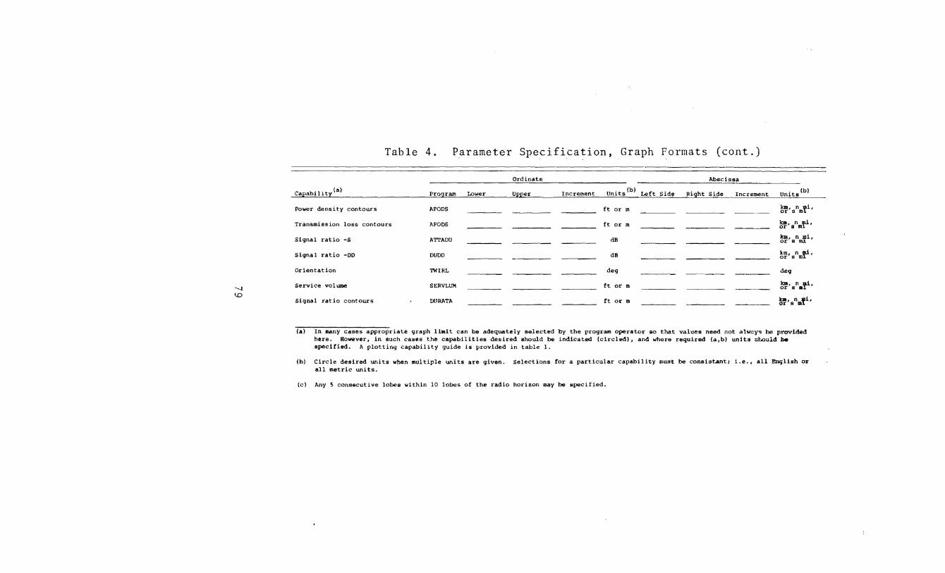
"' \.0
Table 4. Parameter Specification, Graph Formats (cont.)
Ordinate Abscissa
Capahility(al Program Lower Upper Increment Units(b) Left Side Right Side Incre~nt Units(b)
Power density contours A PODS
Transmission loss contours A PODS
Signal ratio -s ATTADU
Signal ratio -DD DUDD -~
Orientation TWIRL
Service volume SERVLUM
Signal ratio contours OORJ\TA
ft or m
ft or m
dB
dB
deg -----ft or m -------ft or m
---~--
~,snrn'fi,
~'snmfl' km, n 111i, or a ou
~'s0mrt'
deq
~, 8n.'fi,
~·snm'fi,
(a) In many cases appropriate graph limit can be adequately selected by the program operator so that values need not alwey~ be provided here. However, in such cases the capabilities desired should be indicated (circled), and where required (a,b) units st~uld be specified. l\ plotting capability guide is provided in table 1.
(b) Circle desired units when multiple units are given. Selections for a particular capability must be conaistant1 i.e., all Enqlish or all metric units.
(c) Any 5 consecutive lobes within 10 lobes of the radio horizon may be specified.
capabilities that involve the use of desired to undesired (D/U)
signal ratios involve two facilities. This includes the last 5
capabilities listed in table 1.
Although about 40 items can be specified with table 2, re
quired specification involves only 3. These "primary parameters"
consist of antenna heights and frequency. Values for "secondary
parameters" will he computed or assumed if not snecified. Para
meter values (or options) that will he assumed in lieu of speci
fication are indicated in the table along with the acceptable
value range (or options available).
The nomenclature used to distinguish between the two anten
nas of a particular path may be misleading to the uninitiated but
is used for convenience. The lower of the two ant~nnas is called
the "facility" even though it may be an aircraft. The other an
tenna must be equal to or higher in altitude than the "facility
or lower" antenna and is designated as the "aircraft" even though
it may be a ground-based antenna or a satellite.
For convenience, the parameters in table 2 are listed alpha
betically within categories. A short discussion of each parameter
is provided in the remainder of this section, and these discus
sions are ordered in accordance with the order of appearance of
the parameter in table 2.
AIRCRAFT OR HIGHER ANTENNA HEIGHT As shown in figure 44, this
altitude is measured above mean sea level (msl). The propagation
model is not valid for antennas located below the surface, and
radio horizons may not be treated correctly if the aircraft alti
tude is less than the facility antenna horizon elevation above
msl. Use of such aircraft altitudes will result in an aborted
run after an appropriate note has been printed on the comnuter
generated parameter sheet (e.g., fig. 1). Notes are printed,
but the run is not aborted if the altitude is (a) less than 1.5
ft (0.5 m) where surface wave contributions that are not included
in the model could become important, or (b) less than the effec
tive reflecting surface elevation plus 500 ft (152 m) where the
80
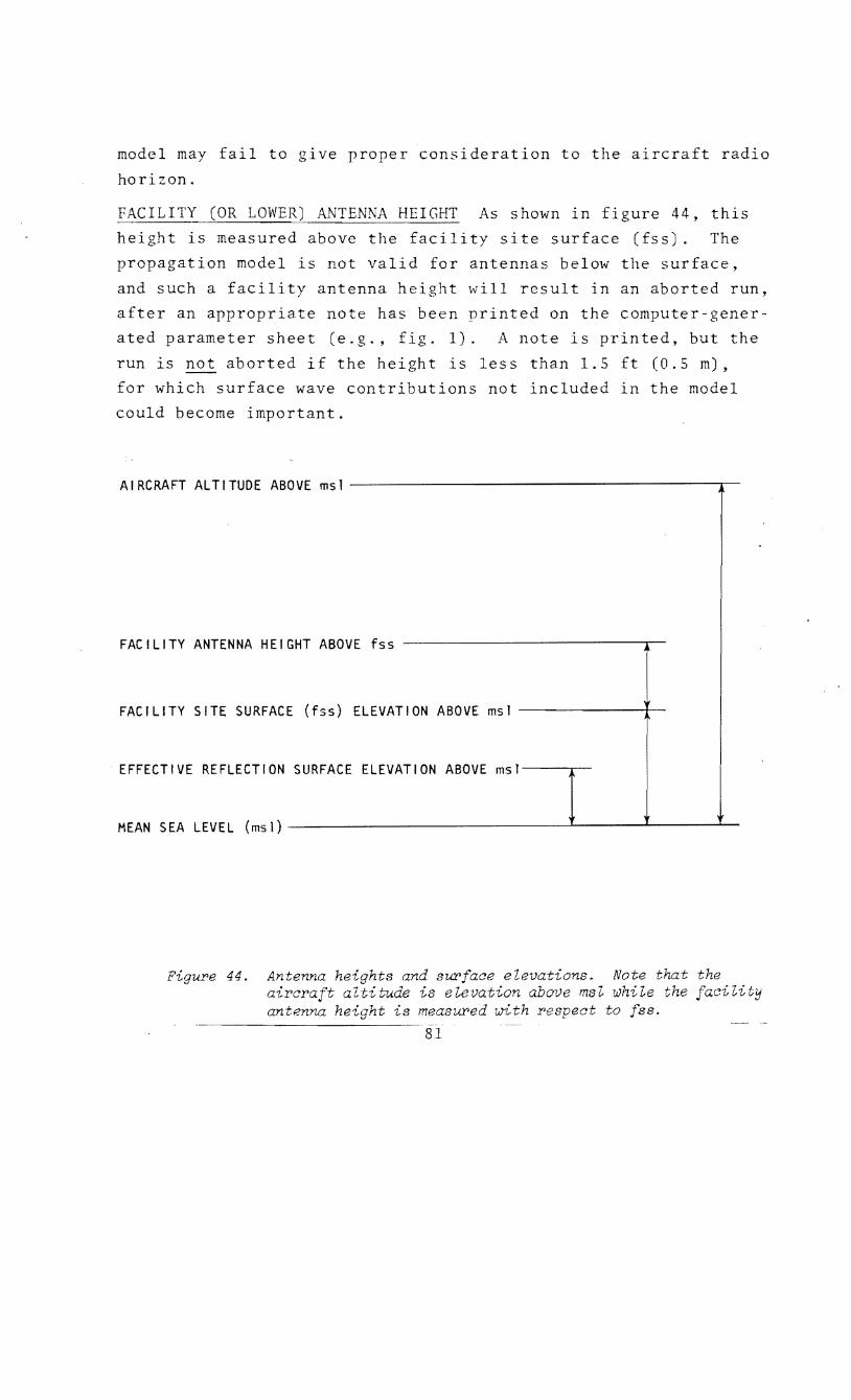
model may fail to give proper consideration to the aircraft radio
horizon.
FACILITY ANTENNA HEIGHT As shown in figure 44, this
height is measured above the facility site surface ( s). The
propagation model is not valid for antennas below the surface,
and such a facility antenna height will result in an aborted run,
after an appropriate note has been printed on the computer-gener
ated parameter sheet (e.g., fig. 1). A note is printed, but the
run is not aborted if the height is less than 1.5 ft (0.5 m),
for which surface wave contributions not included in the model
could become important.
AIRCRAFT ALTITUDE ABOVE msl --------------------------------------.-
FACILITY ANTENNA HEIGHT ABOVE fss
FACILITY SITE SURFACE (fss) ELEVATION ABOVE msl -------------r-
EFFECTIVE REFLECTION SURFACE ELEVATION ABOVE msl----~-
MEAN SEA LEVEL (msi)----------------------------L-----~------~-
Figure 44. Antenna heights and surface elevations. Note that the aircraft altitude is e~evation above ms~ whi~e the faci~ity antenna height is measured with respect to fss.
81

FREQUENCY Notes are printed if the frequency is (a) less than
100 MHz, when neglected ionospheric effects may become important;
(b) greater than 5 GHz, when neglected scattering from hydromete
ors (rain, etc.) may become important; and (c) greater than
17 GHz, when the estimates made for atmospheric absorption may be
inaccurate. For frequencies less than 20 MHz or greater than
100 GHz, the run is aborted.
AIRCRAFT ANTENNA TYPE OPTIONS These options involve the antenna
gain pattern of the aircraft antenna in the vertical plane. Op
tions currently built into the program include isotropic, cosine
(voltage), and JTAC (see eqn. 10) patterns (fig. 45). Program
modifications can easily be made to accommondate other patterns
that are specified in terms of gain versus elevation angle. Hori
zontal (or azimuth) patterns for the aircraft antenna are not
used in any program.
Antenna pattern data are used to provide information on gain
relative to the main beam only. The extent to which the main beam
antenna gain exceeds that of an isotropic antenna is listed in
table 2 as a separate item (i.e., under GAIN) and is included in
the specification of EIRPG (see eqn. 12).
AIRCRAFT ANTENNA BEAM WIDTH This parameter is currently used
only in connection with the JTAC [33, p. 51] antenna pattern
where relative (voltage) gain (g) is a function of the half-power
beam width (eHP), beam tilt above horizontal (et), and the ray
elevation angle (ee) for which g is desired [24, (67)]; i.e.,
g[V/V] = [1 + (2iee-etl/eHP)2.5J -o.s (10)
where ee' et' and eHP must all be expressed in the same units of
angular measure, such as degrees or radians.
AIRCRAFT ANTENNA POLARIZATION IONS Polarization of the air-
craft is not optional. It is always taken as being identical
with that of the facility antenna, which may be specified as cir
cular, horizontal, or vertical. Therefore, losses associated
82
with polarization sense mismatch are not included in the programs.
However, provisions do exist to allow antenna gain patterns for
horizontally and vertically polarization components to be individ
ually specified for calculations involving circular polarization.
AIRCRAFT ANTENNA TILT The aircraft antenna main beam tilt above
horizontal is currently used only with the JTAC antenna pattern
formulation of (10).
AIRCRAFT ANTENNA TRACKING OPTION If this tracking option is
used, the main beam of the aircraft antenna will always point at
the desired facility antenna.
EFFECTIVE REFLECTION SURFACE ELEVATION As shown in figure 44,
this elevation is measured above msl. If not specified, it will
be taken as the terrain elevation above msl of the facility site
surface (fss). This factor is used when the terrain from which
reflection is expected is not at the same elevation as the fa
cility site; e.g., a facility located on a hilltop or cliff edge.
When the elevation of the ility antenna or horizon obstacle
is below the effective reflection surface level, a note will be
printed and the run aborted. This elevation is also used as the
elevation of average terrain for terrain other than the facility
site and horizon obstacle.
The following guidelines are useful in estimating effective
reflecting surface elevations:
1) Do not specify a value for this elevation (then a value equal
to the facility site elevation will be assumed) if (a) terrain in
formation is too di cult to obtain, or (b) the path profile
[49, sec. 6.2] is such that a reasonable estimate is difficult.
For example, do not specify a value when the facility-to-horizon
reflection would be expected to occur from a tilted plane and the
facility horizon obstacle elevation is greater than the facility
site elevation.
2) Take this elevation as the facility horizon obstacle eleva
tion if the path pro le is such that the facility-to horizon re-
flection would be expected to occur from a tilted plane and the
83

horizon obstacle elevation is less than the facility site eleva
tion; e.g., when the terrain slopes downward from the facility
site to its horizon so that none or very little of the terrain be
tween the two has an elevation less than that of the horizon
obstacle.
3) This elevation should, in most cases, be taken as an estimate
of average terrain elevation in the vicinity of the surface along
the great-circle path that is expected to support reflection be
tween the facility antenna and the facility horizon obstacle. In
a plane tangent to the reflecting point, the angle of incidence
should equal the angle of reflection; i.e., grazing angles (w of
fig. 40) are equal at the reflecting point [8, sec. ll.A; 27, sec.
CI-C.2].
The effort required to determine appropriate terrain input
parameters for IF-77 when the first two guidelines are not appli
cable can be very difficult for inexperienced personnel without
adeq~ate tools. Experienced personnel and computer programs use
ful in processing terrain data are available at DOC and should be
utilized for difficult problems.
EQUIVALENT ISOTROPICALLY RADIATED POWER Equivalent isotropically
radiated power (EIRP) is the power radiated from the transmitting
antenna increased by the antenna's main lobe gain; i.e.,
EIRP[dBW] = PTR[dBW] + GT[dBi] (11)
where PTR is the total power radiated from the transmitting an
tenna and GT is the main beam gain of the transmitting antenna.
The term EIRPG is sometimes used (e.g., fig. 16) to indicate EIRP
increased by the receiving antenna main beam gain (GR); i.e.,
EIRPG(dBW] = EIRP[dBW] + GR[dBi]. (12)
In the calculation of transmission loss (e.g., fig. 23) only the
sum of the antenna gains is involved, and the term GAIN is used where
GAIN(dBi] = GT[dBi] + GR[dBi]. (13)
84
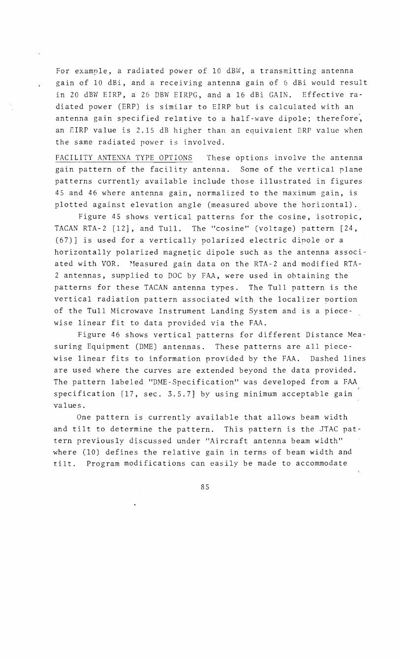
For exam~le, a radiated power of 10 dBW, a transmitting antenna
gain of 10 dBi, and a receiving antenna gain of 6 dBi would result
in 20 dBW EIRP, a 26 DBW EIRPG, and a 16 dBi GAIN. Effective ra
diated power (ERP) is similar to EIRP but is calculated with an
antenna gain specified relative to a half-wave dipole; therefore~
an EIRP value is 2.15 dB higher than an equivalent ERP value when
the same radiated power is involved.
FACILITY ANTENNA TYPE OPTIONS Tl1ese options involve the antenna
gain pattern of the facility antenna. Some of the vertical plane
patterns currently available include those illustrated in figures
45 and 46 where antenna gain, normalized to the maximum gain, is
plotted against elevation angle (measured above the horizontal).
Figure 45 shows vertical patterns for the cosine, isotropic,
TACAN RTA-2 [12], and Tull. The "cosine" (voltage) pattern [24,
(67)] is used for a vertically polarized electric dipole or a
horizontally polarized magne~ic dipole such as the antenna associ
ated with VOR. Heasured gain data on the RTA-2 and modified RTA-
2 antennas, supplied to DOC by FAA, were used in obtaining the
patterns for these TACAN antenna types. The Tull pattern is the
vertical radiation pattern associated with the localizer nortion
of the Tull Microwave Instrument Landing System and is a piece- .
wise linear fit to data provided via the FAA.
Figure 46 shows vertical patterns for different Distance Mea
suring Equipment (DME) antennas. These patterns are all piece
wise linear fits to information provided by the FAA. Dashed lines
are used where the curves are extended beyond the data provided.
The pattern labeled "DME-Specification" was developed from a FAA
specification [17, sec. 3.5.7] by using minimum acceptable gain
values.
One pattern is currently available that allows beam width
and tilt to determine the pattern. This pattern is the JTAC pat
tern previously discussed under "Aircraft antenna beam width"
where (10) defines the relative gain in terms of beam width and
tilt. Program modifications can easily be made to accommodate
85
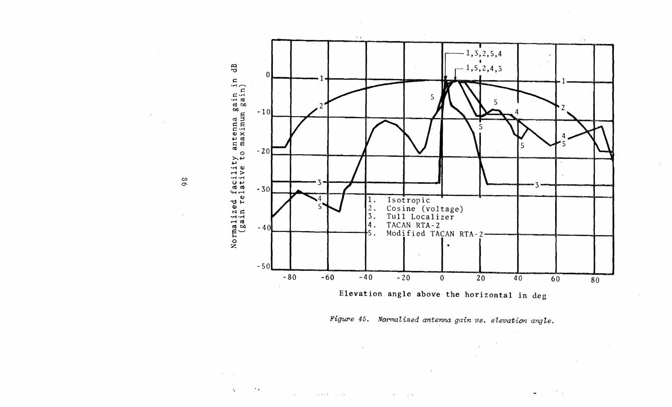
. ' I
r--1,3, I
j:Q
ol I 1 1,5,2,4,3 "'(j
. I I I 1 1 ... I t.:: ·~~
t.:: t.::·~ ·~ o:l
r . 2 o:lbO I bO
E o:l ;:j. t.::E t.::·~ (I) X .f..Jo:l t.::E o:l
0 >...f..J
...... ..... (I)
rl> ·~ ·~ -, I'- I 3
co U.f..J
-30, I 3 I 7 1 I 0\ cdcd 4-1~
(I) '4 1. Isotropic "'(j,... 5 2. Cosine (voltage) (I)
Nt.:: 3. Tull Localizer ·~·~
ricd 4. TACAN RTA- 2 cdbO -40 5 . Modified TACAN RTA-2 S"-' ,...
I I . 0 z
-80 L 1 1 I I 1 I · -so, , • .1.._ 20
40 60 80 -60 -40 -20 0
Elevation angle above the horizontal in deg
Figwe 45. No:r>malized antenna gain vs. elevation angle .
·. . .
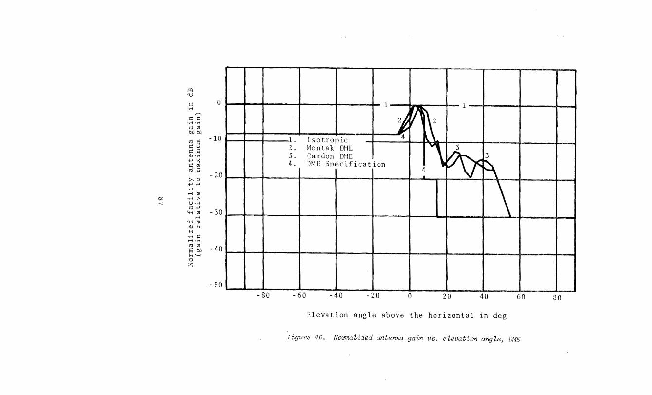
t::Q 'U
~ 0 ·rl
,-... ~ ~
•rl •rl ro ro t.()t.()
1 1
~ zJ; 2
ro s -10 1. Isotronic 4 \ ~;;:l ~ s (]).,...; +.JX ~ro ro s ~0
-20 +J+J •rl ,......((])
00 ·rl ? -..] U·rl
ro+.J 4-1ro -30
,......(
2. fviontak DHE
4\ r\:r 3. Cardon mm 3 4. DME Specification E\ I
l '1:)(]) (])f..< N
·rl ~ ,......( •rl ro ro -40 sc.o f..<'-' 0 z
-so -80 -60 40 -20 0 20 40 60 no
Elevation angle above the horizontal in deg
Figure 46. Normalized antenna gain vs. elevation angle~ DME

other patterns that are specified in terms of gain versus eleva
tion angle.
Program TWIRL is the only program which involves the use of
horizontal plane (azimuth) antenna patterns (see ORIENTATION, fig.
35, discussion in sec. 3.2). An example of such a pattern is the
localizer portion of an ILS 8 loop array antenna (22, fig. 1].
This pattern and preliminary patterns for other ILS localizer
antennas are currently available, but program modifications can
easily be made to accommondate other patterns that ar~ snecified
in terms of gain versus azimuth angle. Antenna pattern data are used to provide information on gain
relative to main beam only'. The extent to which the main beam
antenna gain exceeds that of an isotropic antenna is listed in
table 2 as a separate item (i.e., under GAIN) and is used in the
specification of EIRP as per (11) when the antenna is transmitting.
FACILITY ANTENNA BEAM WIDTH This parameter is currently used
only in connection with the JTAC antenna pattern given by (10).
FACILITY ANTENNA COUNTERPOI ER The counterpoise was in-
corporated into the model for the VOR. It will not be included
in the calculations if its diameter is specified as zero, and the
parameters associated with it will not be printed. A diameter
greater than 500 ft (152 m) will cause a warning note to be
printed, but will not abort the run.
FACILITY ANTENNA COUNTERPOISE HEIGHT If the counterpoise height
above the facility site surface ( s) is less than zero, it will
be set equal to zero. An appropriate note will be printed and
the run aborted if the height is (a) greater than 500 ft (152 m),
or (b) greater than the facility antenna height. The facility
antenna should be above the counterpoise by at least one-third
of a wavelength, which is 3 ft (1 m) at 100 MHz, and by not more
than 2,000 ft (610 m).
88

FACILITY ANTENNA COUNTERPOISE SURFACE OPTIONS Counterpoise sur-
face options fix the conductivity and dielectric constant associ
ated with the counterpoise surface. Values associated with each option are given in table 5.
FACILITY ANTENNA ZATION OPTIONS These options include circular , horizontal, and vertical polarization [47, ch. 8].
Polarization for the aircraft antenna is always taken as being
identical with that of the fa~ility antenna. Therefore, losses
associated with polarization sense mismatch are not included in
the programs. However, provisions do exist to allow antenna gain
patterns for horizontally and vertically polarized components to
be individually specified for calculations involving circular polarization.
FACILITY ANTENNA TILT The facility antenna main beam tilt above·
horizontal is currently used only with the JTAC antenna pattern
formulation of (10). However, it can also be used to adjust the" tilt of other patterns.
FACILITY ANTENNA TRACKING OPTION If this tracking option is
used, the main beam of the facility antenna will al~ays point at the aircraft.
Table 5. Surface Types and Constants
[25, table 6]
Type
Poor ground
Average ground
Good ground
Sea water
Fresh water
Concrete Metal
Conductivity (mhos/m)
0.001
0.005
0.02
5*
0.01*
0.01
10 7
Dielectric Constant
4
15
25 81*
31*
5
10
*More appropriate values are calculated if surface sea tempera
ture is specified.
89
FREQUENCY FRACTION This is the fraction of the carrier frequency
that corresponds to half the bandwidth used for the spectral plot
capability (fig. 15). For example, a carrier frequency of 125 MHz
and a fraction of 0.0004 would result in a bandwidth of
( 2) ( 0 . 0 0 0 4 ) (12 5) = 0 . 1 MH z = 1 0 0 kH z .
GAIN, RECEIVING ANTENNA This item is the main beam gain [dBi]
of the receiving antenna. A 0 dBi value will be assumed if no gain is specified.
GAIN, TRANSMITTING ANTENNA This item is the main beam gain
[dBi] of. the transmitting antenna. A 0 dBi value will be assumed
if no gain is specified.
TRANSMITTING ANTENNA LOCATION This item is included to provide
a more complete specification of problem parameters and to allow
the program operator to check for potential incorrect power den
sity or D/U estimates. Other predictions have transmitter/receiver reciprocity. Power density and D/U calculations assume
that the transmitting antenna is located at the facility.
HORIZON OBSTACLE DISTANCE FROM FACILITY If not specified, this
distance will be calculated from horizon parameters that are spec
ified and/or by using the terrain uarameter Ah. When the dis
tance is not within 0.1 to 3 times the smooth earth horizon dis
tance, a warning note will be printed, but the run will not be aborted.
HORIZON OBSTACLE ELEVATION ANGLE ABOVE HORIZONTAL AT FACILITY
If not specified, the horizon obstacle elevation angle at the
facility will be calculated from horizon parameters that are spec
ified and/or by using the terrain parameter Ah. When the angle
exceeds 12°, a warning note will be printed, but the run will not be aborted.
HORIZON OBSTACLE HEIGHT If not specified, this height will be calculated from horizon parameters that are specified and/or by using the terrain parameter Ah. When the height is not within
90
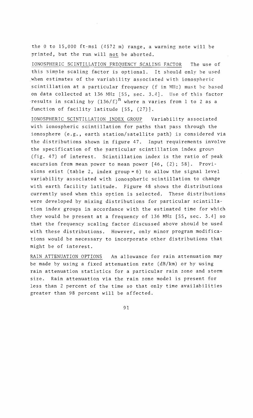
the 0 to 15,000 ft-msl (4572 m) range, a warning note will be
printed, but the run will not be aborted.
IONOSPHERIC SCINTILLATION FREQUENCY SCALING FACTOR The use of
this simnle scaling factor is optional. It should only be used
when estimates of the variability associated with ionospheric
scintillation at a particular frequency (f in ~fll:) must he based
on data collected at 136 MHz [55, sec. 3.4]. Use of this factor
results in scaling by (136/f)n where n varies from 1 to 2 as a
.function of facility latitude [55, (27)].
IONOSPHERIC SCINTILLATION INDEX GROUP Variability associated
with ionospheric scintillation for paths that pass through the
ionosphere (e.g., earth station/satellite path) is considered via
the distributions shown in figure 47. Input requirements involve
the speci cation of the particular scintillation index groun (fig. 47) of interest. Scintillation index is the ratio of peak
excursion om mean power to mean power [46, (2); 58]. Provi
sions exist (table 2, index group= 6) to allow the signal level
variability associated with ionospheric scintillation to change
with earth facility latitude. Figure 48 shows the distributions
currently used when this option is selected. These distributions
were developed by mixing distributions for particular scintilla
tion index groups in accordance with the estimated time for which
they would be present at a frequency of 136 MHz [55, sec. 3.4] so
that the frequency scaling factor discussed above should be used
with these distributions. However, only minor program modifica
tions would be necessary to incorporate other distributions that
might be of interest.
RAIN ATTENUATION OPTIONS An allowance for rain attenuation may
be made by using a fixed attenuation rate (dB/km) or by using
rain attenuation statistics for a particular rain zone and storm
size. Rain attenuation via the rain zone model is present for less than 2 percent of the time so that only time availabilities greater than 98 percent will be affected.
91
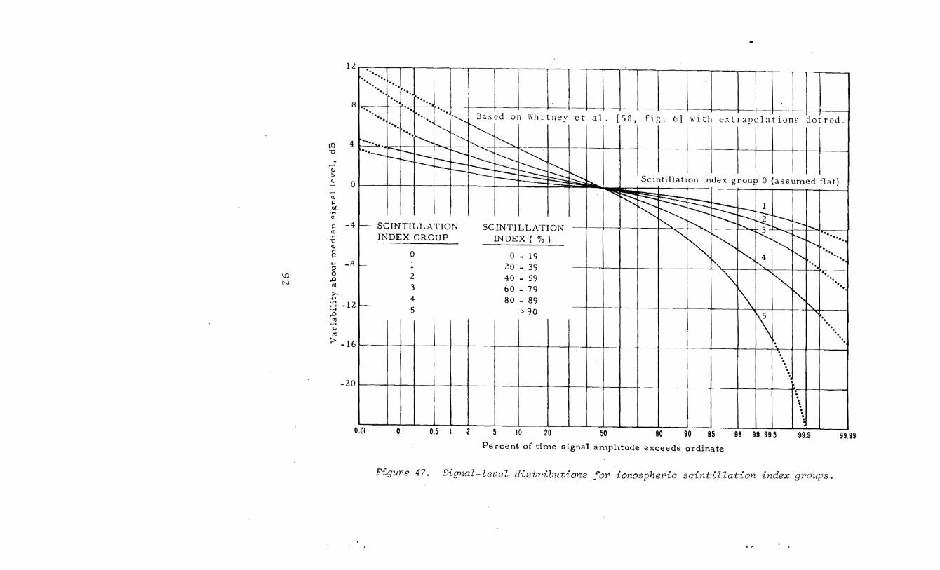
l.C
8
~ 4 "C
...... <lJ > il.l 0 ......
..... Cll ~ at ..... "'
SCINTILLATION SCINTILLATION INDEX ( %} INDEX GROUP
:;:: -4 <11 .....
"C (!)
E 0 0 - 19 20 - 39 1 ..... -8 ::s 40 - 59 2
60 - 79 3
80 - 89 4
> 90 5
'-0 0 N .D
ro >-..... a -12
.D <11 ..... l-t <1l
> -16
-20
0.01 0.1 0.5 2 5 10 20 50 80 90 95 98 99 99.5 99.9 99.99 Percent of time signal amplitude exceeds ordinate
Figure 47. Sign.al-level distributions for ionospheY'ic scintillation index gY'oups.

(.Q
tN
.-i <lJ 2 > <lJ
.-i
.-i ttl 0 1:: 0.';
•rl (/)
6
~ ~ ~ ~ ~ ~ ~--- .... 1-- --- r---~
!"-~""'·· ~ ~
~ ~ ~ ~ - R ~ ~
~ -..;;;: r'--... ~"'-....... r-..... ~ -+- ......... r-..... i""--- .....
4
1::
.~ -2 "d
<lJ E
.... ~ -4
..0 ttl
>-. .... •rl -6 .-i •rl .c ttl
•rl f.< (\j -8 >
-10
-~ ~ ~- I ......;:
~ ~~ ~ r\ 1"--,
'\~ !'\~ .. ~ ·~ -t-- ---!----
\ ' -~-
' ' ' I\' -+-
~ ~ ~-North latitude
OQ --- -· \ i\\
5 Q _,_,_,_,_, ___ - - --- f--
I 1o· \ \~ I
14° -~--- ~ i\ ~ i -I 17-52° --- ~ --f-~ -~
~ ~ \ 57 (I ---------
60 ° ..........................
- 1":_
0.01 0.1 0.5 l 2 5 10 20 50 80 90 95 98 99 99.5 99.9 99.99
Percentage of time signal amplitude exceeds onlinatc
Figure 48. Signal-level distributions currently used with variable scintillation group option selected. These distributions were developed from data co~l?~teg at 136 MHz [55~ sec. J.4] so that the frequency scaling factor should be used with them.
""
RAIN ATTENUATION/KM With this option, rain attenuation is cal culated as the product of the attenuation rate and the length of
the most direct ray path between the terminals that is within the
storm.
RAIN STORM SIZE This is the length (or diameter) of the storm
over the great-circle path connecting the terminals. It is as
sumed that this length is made up by a single storm that extends
to an altitude above average terrain that is equal to the storm
size and contains as much of the most direct ray nath as possible.
For the models used here the greatest length of path subjected to
rain attenuation is limited to the rain storm length and the smal
lest is zero since the direct ray could be entirely above the
storm for an air-to-air propagation path.
RAIN ZONE If the option involving
is desired, a rain zone number from
tinental United States or figure 50
is selected [51, 52, 53,- 54, 57].
statistical attenuation rates
either figure 49 for the con
for other parts of the world
Rain attenuation
tion is present for less than 2 percent of the time
time availabilities greater than 98 percent will be
via this op
so that only
affected.
REFRACTIVITY Values for the minimum monthly mean surface refrac
tivity referred to mean sea level (N ) may be estimated from ei-o
ther figure 51 for the continental United States or figure 52 for
other parts of the world. Other information [3, 4, 5, SO, 51, 52]
which may be more appropriate for the particular conditions (e.g.,
time of year and location) involved can be used to estimate N0
or a minimum monthly mean value for effective earth radius. Spec
ification of N outside the 200-to-400 N-unit range will result 0
in N being set to 301. If 0
the surface refractivitv (N ) calcu-' s
lated [49, (4.3)] from N 0
is less than 200 N-units, N will be s
set to 200 N-units and an appropriate note printed. An N of 301 s N-units corresponds to a~ effective earth radius factor of 4/3
[49, fig. 4.2], If desired, a value for effective earth radius
can be specified directly.
94
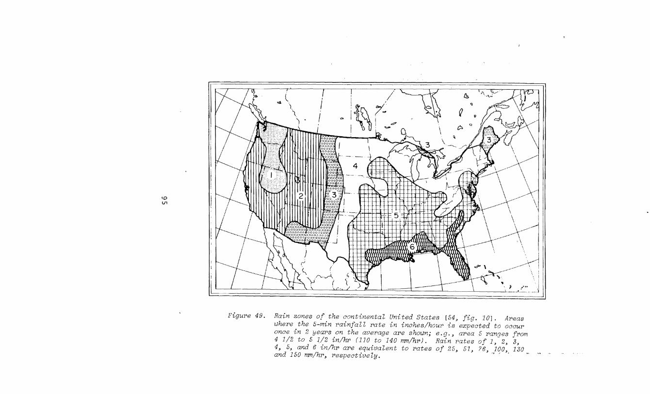
1.0 Ul
..s ( I
') ' i& /~ I
'\ ) . I . 1\~7- o.
~ Q
I I -.?
q
. h. a \ £:::, <:)
~
Figure 49. Rain zones of the continental United States [54, fig. 10]. Areas where the 5-min rainfall rate in inches/hour is expected to occur once in 2 years on the average are shown; e.g., area 5 ranges from 4 1/2 to 5 1/2 in/hr (110 to 140 mm/hr). Rain Y'ates of 1, 3, 4, 5, and 6 in/hr are equivalent to rates of 25, 51, ?6, 100, 130 and 150 mm/hr, respectively. ., ' '
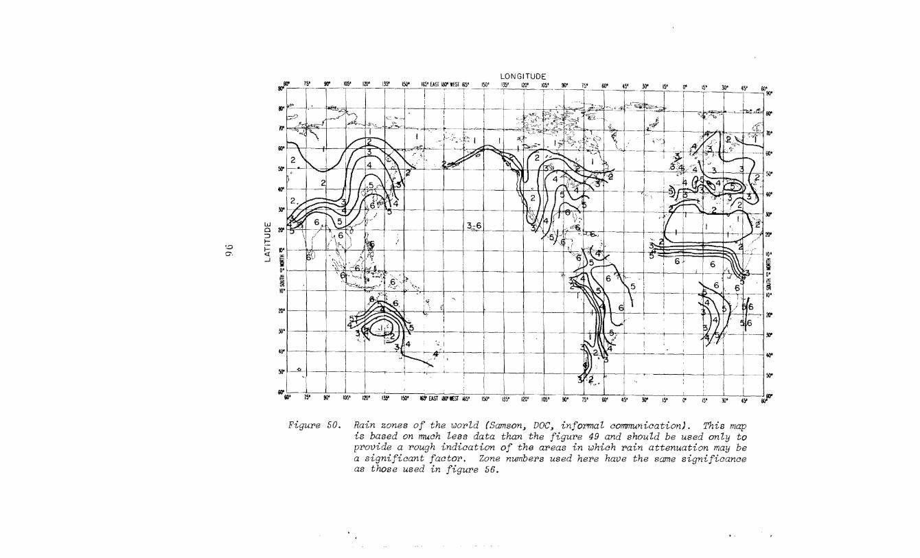
·-:::;~
~ ".
~ w ~ • ~ ~ ~ ~~~6-00'r- -r--,-T-iT ---,-
JO•
. ----'--t l >' ~ I 5o-
40'
w g --I'"' \1 I'L h.~v h I . I i I I . . V«'C~p:.:&;-r--,----,--- I I I I I I ~,-l:T-tl 20' i 1-
!;r - I _J &j. ~{) !. I ,., 1 I I I I I r~-r"":-61\'~ l-l~+.::l I _ ~~r-ii
o•
10' L I ;j 6' ·[ I d.~ ' " \•_, i I I I I I I ~~~0 '\5'i I 'l_Gl ~l -~~
20'
lO'
40'
50"
00' • • ~ ~ eoo~~• ~ ~ w • 4~ fll'fll'
Figu~e 50. Rain zones of the wo~td (Samson, DOC, informal communication). This map is based on much tess data than the figu~e 49 and should be used onty to p~ovide a ~ough indication of the ~eas in which ~ain attenuation may be a significant facto~. Zone numbe~s used he~e have the same significance as those used in figu~e 56.
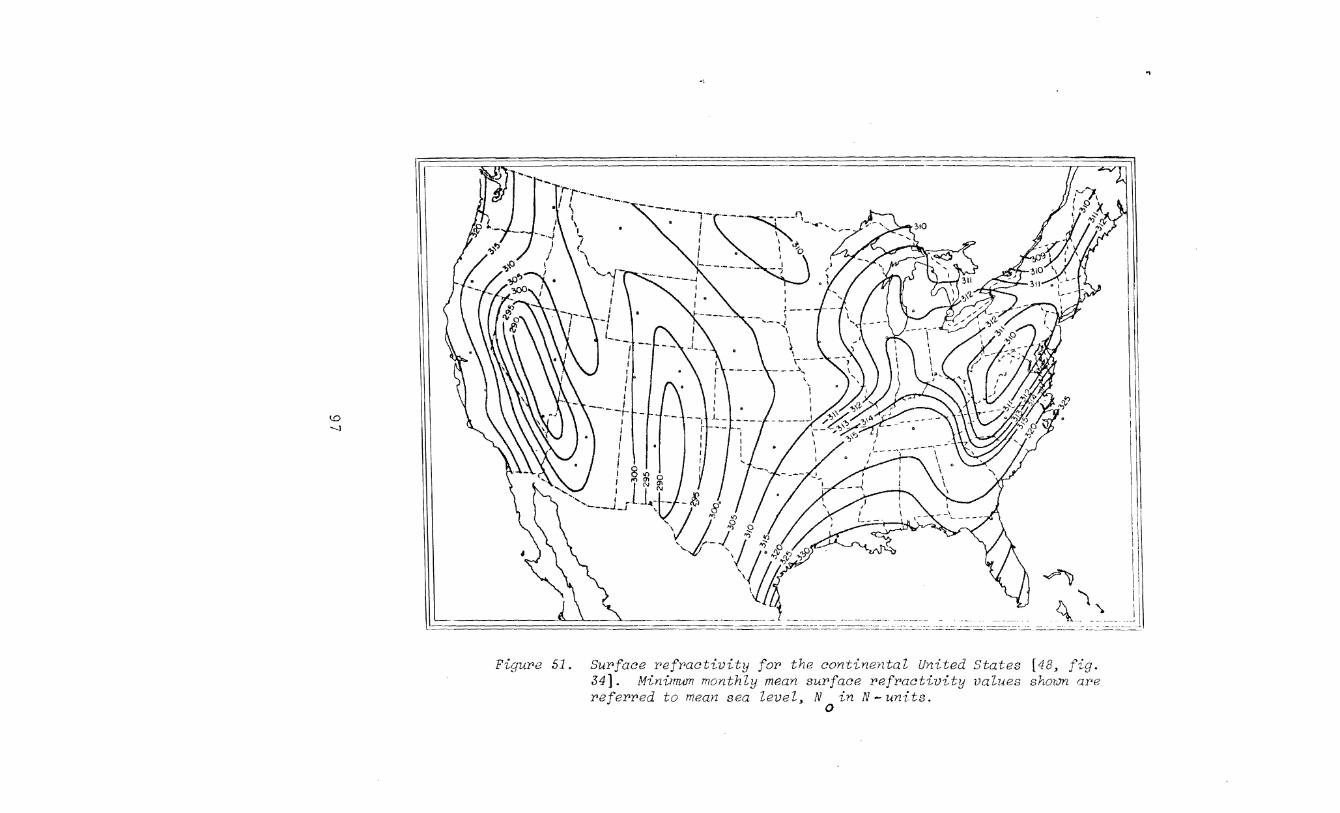
\0 '-)
·-·----~---.-·-·-('1·-· ... -' ... ~I \ .r ! '0 I I ·-,
...r'"~
~'~ Figur>e 51. Sur>face Pefr>activity for> the continental United States [48, fig.
34]. Minimum monthly mean sur>face r>efr>activity values shown aPe r>efeY'Ped to mearz sea level, N in N-unlts.
0
.,
I

120 100 eo 60 40 20 w o E 20 40 ro eo 100 120 140 1so E 100 .--.~--r-,--,--,-,--,--,-,
N
~ ~
ro ro
60 60
50 50
40 40
w ~
20 20
10 10 H N
<.0 I o o co s s
tit
10 10
20 20
~ ~
40 40
50 50
60 --,~~ 60 . '-..., _.-1305
':j""""":j::::,=F==::t::::::>,_, ....e-t::::::- -...-- I
70 ---~~== 70
eo ·---~~= eo s ' I S
Figure 52. Surface refractivity for the world [49> fig. 4.1]. Minimum monthly mean surface refractivity values are referred to mean sea level~ N in N-units.
0
..
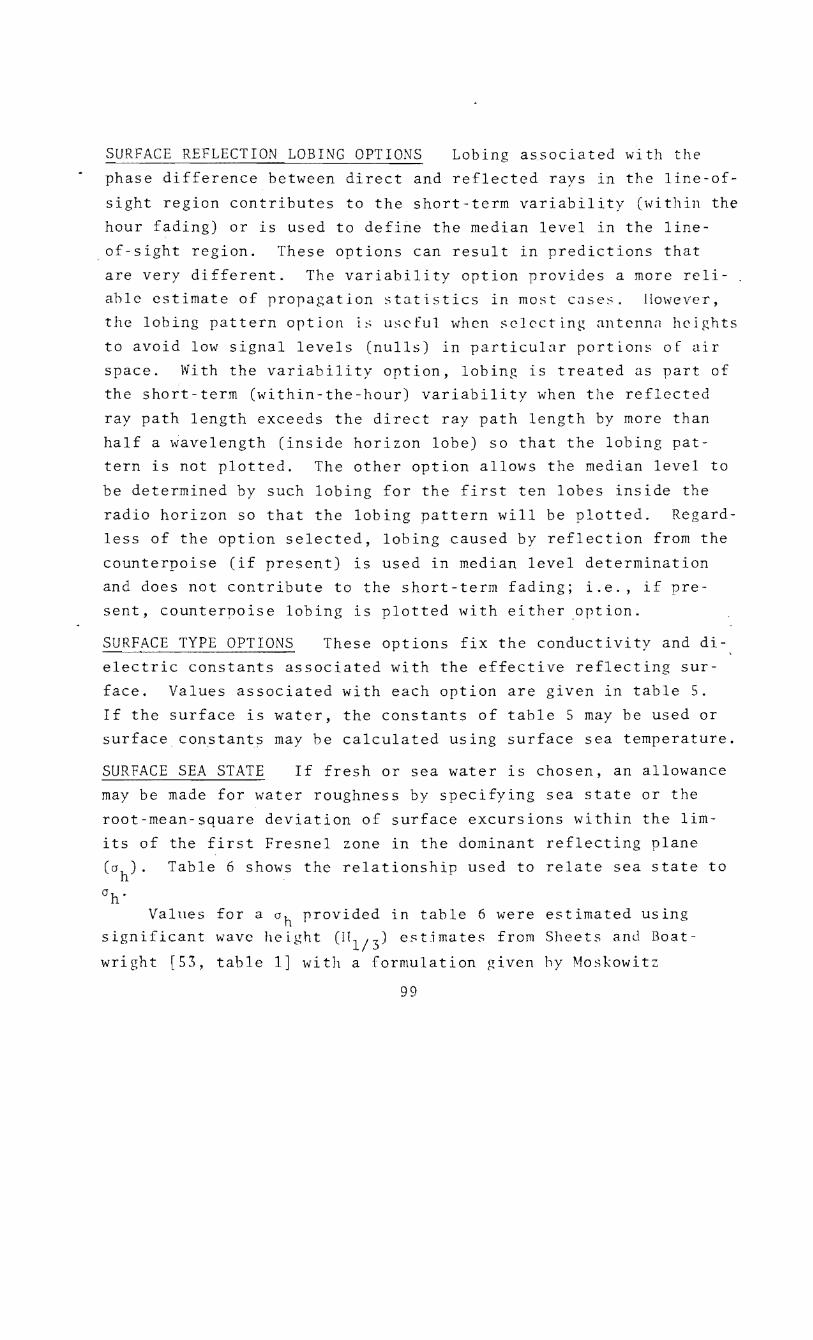
SURFACE REFLECTION LOBING
phase difference between
Lobing a~sociated with the
reflected rays in the line-of-
sight region contributes to the short-term variability (within the
hour fading) or is used to define the median level in the line-
. of-sight region. These options can result in predictions that
are very different. The variability option provides a more reli
able estimate of propagation statistics in most cases. l!owever,
the lobing pattern option is useful when selecting antenna heights
to avoid low signal levels (nulls) in particular portions of air
space. With the variability option, lobing is treated as part of
the short-term (within-the hour) variability when the reflected
ray path length exceeds the direct ray path length by more than
half a wavelength (inside horizon lobe) so that the lobing pat
tern is not plotted. The other option allows t median level to
be determined by such lob for the first ten lobes inside the
radio horizon so that the lobing pattern will be plotted. Regard
less of the option selected, lobing caused by reflection from the
counterpoise (if present) is used in median level determination
and does not contribute to the short-term fading; i.e., if pre
sent, counternoise lobing is plotted with either .option.
SURFACE TYPE OPTIONS These options fix the conductivity and di
electric constants associated with the effective reflecting sur
face. Values associated with each option are given in table 5.
If the surface is water, the constants of table 5 may be used or
surface constants may be calculated using surface sea temperature.
SURFACE SEA STATE If fresh or sea water is chosen, an allowance
may be made for water roughness by specifying sea state or the
root mean-square deviation of surface excursions within the lim
its of the first Fresnel zone in the dominant reflecting plane
(ah). Table 6 shows the relationship used to relate sea state to
ah. Values for a oh provided in table 6 were estimated using
significant wave height (IT 113 ) est.imates from Sheets and Boat-
wright [53, table 1] with a formulation given hy Moskowitz
99

Table 6. Estimates of ah for Sea States [27r p. CI-81].
(a) Sea State Code
0
1
2
3
4
5
6
7
8
9
. t' (a) Descr1p 1ve Terms
Calm (glassy)
Calm (rippled)
Smooth (wavelets)
Slight
Moderate
Rough
Very rough
High
Very high
Phenomenal
Average Wave Height Range Meters (feet)
0 (0)
0 - 0.1 (0 - 0.33)
0.1 - 0.5 (0.33 - 1.6)
0.5 - 1.25 (1.6 - 4.0)
l. 25 - 2. 5 (4 - 8)
2.5 - 4 (8 - 13)
4 - 6 (13 - 20)
6 - 9 (20 - 30)
9 - 14 (30 - 46)
>14 (>46)
H 113
(b)
Meters
0 (0)
0.09 (0. 3)
0.43 (1.4)
1 ( 3. 3)
1.9 (6 .1)
3 (10)
4.6 (15)
7.9 (26)
12 (40)
>14 (>45)
(feet)
(a) Based on international meteorological code [42, code 3700].
Meters (feet)
0 ( 0)
0.00 (0.08)
0.11 (0.35)
0.25 (0.82)
0.46 (1. 5)
0.76 (2. 5)
1.2 ( 3. 8)
2 ( 6. 5)
3 (10)
>3.5 (>11)
(b) Estimates significant wave heights, average of highest one-third, HI [53, table 1].
1 3
(c) Estimated using a formulation provided by Moskowitz [41, (1)] with H I estimates.
1 3
100
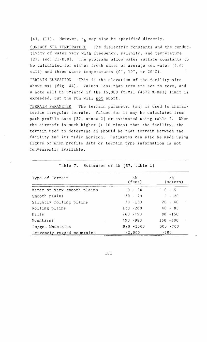
[41, (1)]. However, oh may also be specified directly.
SURFACE SEA TEMPERATURE The dielectric constants and the conduc
tivity of water vary with frequency, salinity, and temperature
[27, sec. CI-D.8]. The programs allow water surface constants to
be calculated for either fresh water or average sea water (3.6%
salt) and three water temperatures (0°, 10°, or 20°C).
TERRAIN ELEVATION This is the elevation of the facility site
above msl (fig. 44). Values less than zero are set to zero, and
a note will be printed if the 15,000 ft-msl (4572 m msl) limit is
exceeded, but the run will not abort.
TERRAIN PARAMETER The terrain parameter (tih) is used to charac
terize irregular terrain. Values for it may be calculated from
path profile data [37, annex 2] or estimated using table 7. ~~en
the aircraft is much higher > 10 times) than the facility, the
terrain us to determine tih should be that terrain between the
facility and its radio horizon. Estimates can also be made using
gure 53 when profile data or terrain type information is not
conv~niently available.
Table 7. timates of tih [37, table 1]
Type of Terrain tih tih
Water or very smooth plains 0 - 20 0 - 5
Smooth plains 20 - 70 5 - 20
Slightly rolling plains 70 -130 20 40
Rolling plains 130 260 40 - 80
Hills 260 -490 80 150
Mountains 490 -980 150 -300
Rugged Mountains 980 -2000 300 -700
101
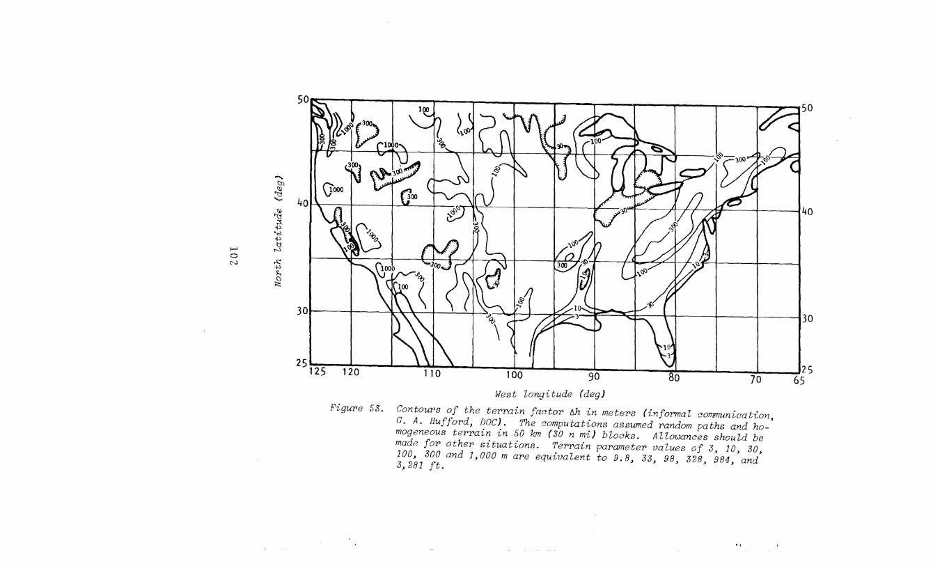
...... (:n (I)
'1j ....... (I)
'1j ;:i
-{.:!
'..:> -{.:!
1-' tj
N 0 N ~
~ ~ ;g
'iUI \ fl I I"' I ~, ,, v .. ~ " I I V .>OI'>Il~ 4 I L fi-t:-' TTl 7 I
30.
25 --
- - . -, --~·······-· . ._ . . .
120 110 100 90 70 West longitude (deg)
FiguPe 53. Contours of the tePPain factoP ~h in metePs (infoPmal communication, G. A. HuffoPd, DOC). The computations assumed Pandam paths and homogeneous tePPain in 50 km (30 n mi) blacks. Allowances should be made foP otheP situations. TePPain paPameteP values of 3, 10, 30, 100, 300 and 1,000 m ape equivalent to 9.8, 33, 98, 328, 984, and 3,281 ft.
. '
~40
"30
25 65
TERRAIN TYPE OPTIONS If the smooth earth option is select
all calculations will be based on smooth earth parameters even
though parameters specified elsewhere imply irregular terrain.
For example, smooth earth specification would cause specified hor
izon parameters to be neglected and smooth earth values us in
their place.
TIME AVAILABILITY OPTIONS If the first option is selected,
short-term (within the-hour) fading will contribute to the vari
ability, and time availability is applicable to instantaneous lev
els that are available for specific percentages of the time. With
the second option, only long-term (hourly median) variations are
included in the variability, and time availability is applicable
to the hourly median levels that are available for a specific nercentage of hours.
TI~fE AVAILABILITY CLIMATES OR TIME BLOCKS If no option is sele~
ted under climates, the programs will use the long term (hourly
median) variability as described in Gierhart and Johnson [24,
sec. A.S]; i.e., continental all year climate. Climates similar
to those defined by the CCIR [9] and described in table 8 are
available. Variability functions for these climates were devel
oped at the DOC (informal communication, A. G. Longley and G. A.
Hufford). The factor used in the propagation model to avoid ex
cessive variability for paths with a very high antenna (satellite)
was developed for the continental all year climate [23, fig. 2],
and the use of other climates for satellite paths may result in
excessive variability. Time blocks for the continental temperate
climate also are options. The time block periods are defined in
table 9.
4.2 SPECIAL PARAMETERS (Table 3, p. 76)
Special parameters required for particular capabilities are
covered in table 3. Some of these parameters are required for
more than one capability, and the 13 capabilities associated with
programs LOBING and ATOA (table 1) do not require parameters from
103
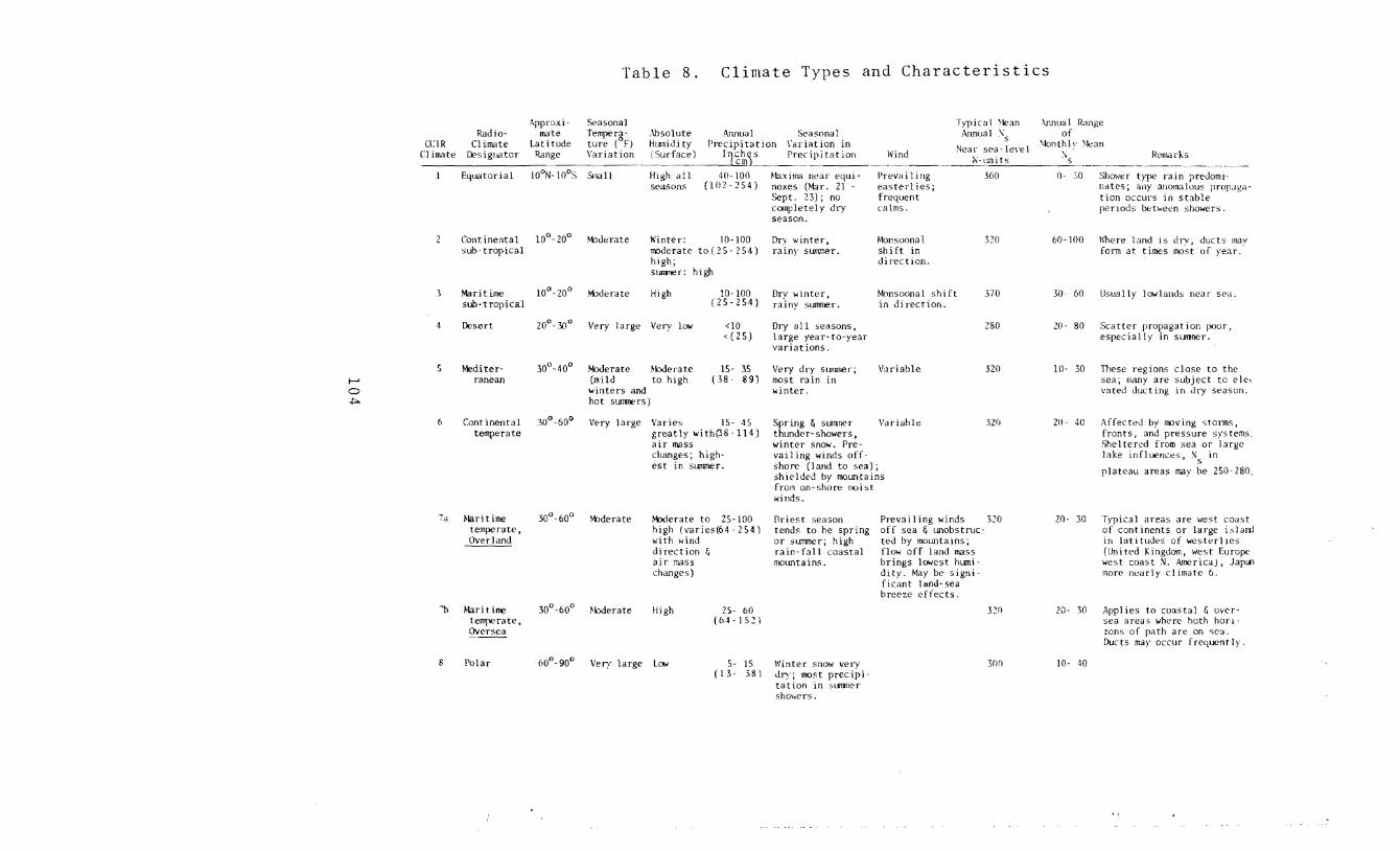
t-o ~
Table 8. Climate Types and Characteristics
Approxi- Seasonal Radio- mate Tempera- Annual Seasonal
CCIR Climate Latitude ture (°F) \'ariation in
~lean \ . s
Climate IX>sigwtor Range Variation Precipitation ----- --------
\'lind Near sea -1e,·e 1 --- _____ "-:_u=ni.:..t::_s ___ _
-\nnua 1 Range of
\fonthh· ~lean \.
s Remarks
6
Equatorial l00N-100S Small High all 40-100 ~axima near seasons (1 0 2 2 54) no xes (Mar.
Sept. 23) ; no complete! y dry season.
Continental 10°-20° '4:ld.,rate Winter: 10-100 Dry winter, Monsoonal shift in direction.
suh- tropical mderatc to(ZS 254) rainy summer. high; Slllll!lef: high
Maritime 10°-20° M:Jderate High 10-100 (25-254)
winter, sumner.
Monsoonal shift in direction. sub-tropical
Desert
Mediterranean
Continental temperate
20°- 30° Very large Very low <10 <(25)
30°-40°
30°60°
Moderate (mild winters and hot SUI11l1e rs J
~kxlerate to high
IS- 35 (38- 89)
Very large Varies 15- 45 greatly with(38 114) air mass
high-
Dry all seasons, large year-to-year variations.
Very dry summer; most rain in winter.
Variable
Spring & summer Variable thtmder-showers, "'inter snow. Pre-vai 1 ing winds off· shore (land to sea); shielded by mountains from on- shore moist winds.
360
320
370
280
320
32(J
7a ~larit ime temperate, Overland
30°-60° ~bderate Moderate to 25-100 high (varies(64 254) with wind
flriest season tends to be spring or :;ummer; high rain-fall coastal mountains.
Prevailing winds 320
'b Maritime temperate, OVersea
s Polar
direction & air mass changes)
30°-60° ~kxlerate High
60°·90° Very large LCJN
2S- 60 (M-15~1
5- IS (13- 381
h'inter snow very dry; most precipitation in sunrner sho\~ers.
off sea & unobstructed by mountains; flow off land mass brings lowest htm1idity. May be significant land- sea breeze effects.
32n
3fln
0- 30 Shower type rain nates; any anomalous propJgation occurs in stable periods between showers.
60-100 \\'here land is dry, ducts may form at t irocs most of rear.
30 60 Usually lowlands near sea.
20- 80 Scatter propagation poor, especially in summer.
10- 30
211- 40
20- 30
These reg ions close to the sea, many are subject to eleo vated ducting in dry season.
Affected by roving ston!Ls, fronts, and pressure Sheltered from sea or lake influences, ~s in
plateau areas may be 250-280.
areas are west coost continents or large islan:J
in latitudes of westerlies (United Kingdom, west Europe west coast~- America), Japon more nearly climate 6.
20- 30 Applies to coastal & oversea areas where hoth hon · zons of path are on sea. Ducts mar occur frequent I r.
10- 40
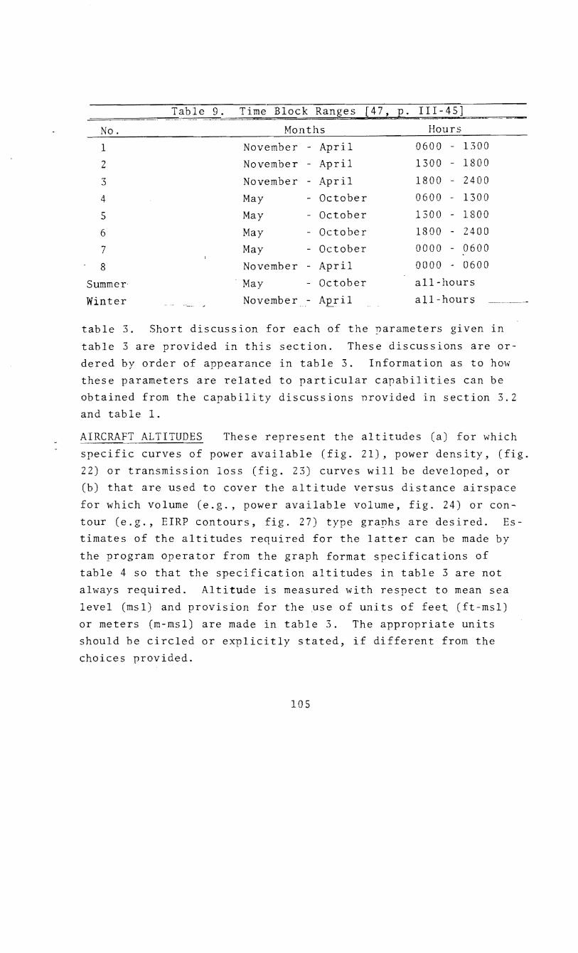
Table 9 • Time Block Ranges [47, E· III-45]
No. Months Hours
1 November - April 0600 1300
2 November April 1300 - 1800
3 November - April 1800 2400
4 May - October 0600 - 1300
5 May - October 1300 - 1800
6 May October 1800 - 2400
7 May - October 0000 0600
8 November April 0000 - 0600
Summer May - October all-hours
Winter November - April all-hours --·-··-
table 3. Short discussion for each of the parameters given in
table 3 are provided in this section. These discussions are or
dered by order of appearance in table 3. Information as to how
these parameters are related to particular capabilities can be
obtained from the capability discussions nrovided in section 3.2
and table 1.
AIRCRAFT ALTITUDES These represent the altitudes (a) for which
specific curves of power available (fig. 21), power density, (fig.
22) or transmission loss (fig. 23) curves will be developed, or
(b) that are used to cover the altitude versus distance airspace
for which volume (e.g., power available volume, fig. 24) or con
tour (e.g., EIRP contours, fig. 27) type graphs are desired. Es
timates of the altitudes required for the latter can be made by
the program operator from the graph format specifications of
table 4 so that the specification altitudes in table 3 are not
always required. Altitude is measured with respect to mean sea
level (msl) and provision for the ~se of units of feet (ft-msl)
or meters (m-msl) are made in table 3. The appropriate units
should be circled or explicitly stated, if different from the
choices provided.
105
TIME AVAILABILITY The specification of time availability (see sec. 4.1, TIME AVAILABILITY ... discussions) is required for those
capabilities where a single time availability is used. It may range from 0.01 to 99.99 percent. Statistical rain attenuation effects will only be present for time availabilities greater than
98 percent (see sec. 4.1, RAIN ZONE discussion). A time availability of 95 percent will be used when another value is not specified.
POWER AVAILABLE, POWER DENSITY, TRANSMISSION LOSS AND/OR EIRP Single and/or multiple values of power available, power density,
transmission loss, and/or EIRP are needed for several capabili
ties.
STATION SEPARATION The specification of station separation (fig.
42) is required for those capabilities where a single station
separation is used. The appropriate units should be circled or explicitly stated, if different from the choices provided.
DESIRED FACILITY-TO-AIRCRAFT DISTANCE This distance is re-
quired for the Signal Ratio-S (fig. 33) capability where the
location of the aircraft is fixed (altitude and distance) rela
tive to the desired facility. The appropriate units should be
circled or explicitly stated, if different from the choices provided.
DESIRED-TO-UNDESIRED SIGNAL RATIO Specification of desired-
to-undesired signal ratio (D/U) is required for those capabilities where a single D/U ratio is u~ed.
PROTECTION POINT LOCATIONS Protection point locations must be specified for the orientation capability. Th~se points are
located relative to the desired facility as illustrated in figure 43 with angles relative to the desired facility course
line, and desired facility to protection point distance. Pro
tection point locations will be taken as those associated with figure 43 when they are required, but not specified. The appropriate units should be circled or explicitly stated, if
different from the choices provided. 106
4.3 GRAPH FORMAT PARA~1ETERS (Table 4, p. 78)
Parameters associated with graph formats are covered ln ta
ble 4. In many, if not most, cases, an adequate selection of
these parameters can be made by the program onerator so that
complete specification via table 4 is not often required.
Some graphs have options associated with the ordinate (feet
or meters) and/or abscissa (degrees, kilometers, nautical miles,
or statute miles) units. These options are selected via table 4
by circling the choice desired. The degrees option involves the
use of central angle instead of path distance (fig. 41). This
option is useful when coverage estimates for a geostationary
satellite are required.
Except for the spectral plot capability, the parameters re
quired for table 4 are associated with the ordinate (lower-to
upper) and abscissa (left-to-right) scales. End points, incre
ment between grid lines, and units are specified. The interval
between end points should correspond to an integer number of increments. Except when transmission loss is plotted, the unner
value should exceed the lower value. In all cases, the right
value should exceed the le value and values less than zero
should not be used.
Spectrum plots may be made with the spectral nlot capability
for any 5 consecutive lobes within 10 lobes of the radio-horizon where the first lobe is taken as the first lobe inside the radio
horizon (see SPECTRAL PLOT, fig. 15, discussion ln sec. 3.2).
For example, speci cation to "plot lobe 3 through 7" would re
sult in plots for lobes 3, 4, 5, 6, and 7.
5. SUMMARY AND SUBMISSION INFORMATION
The ten computer programs covered by this report are useful
in estimating the service coverage of radio systems operating in
the frequency band from 0.1 to 20 GHz. These programs and the propagation models (sec. 2) used in them are extensions of work
previously reported [24; 25, sec. CII]. They may be used to
107
obtain a wide variety of computer generated microfilm plots.
Plotting capabilities are summarized in table 1 and discussed in
section 3.2. Sample graphs are provided in section 3.1 and sam
ple problem applications are given in section 3.3. Concise in
formation on input parameter requirements is provided in tables 2
through 4 (sec. 4)
A potential user should
1) read the brief description of the propagation model
provided in section 2 to see if the model is anpli
cable to his problem,
2) select the program(s) whose output(s) are most apnro
priate from the information given in section 3 (ta
ble 1),
3) determine values for the input parameters discussed
in section 4 (table 2 through 4),
4) request a cost estimate for appropriate computer
runs, and
5) submit the formal request and/or purchase order that
may be required.
FAA requests should be addressed to:
Federal Aviation Administration Spectrum Management Staff, ARD-60 Systems Research and Development Service 2100 Second Street, S.W. Washington, D. C. 20591
Attention: Navigation Specialist
Telephone contact is strongly encouraged, and Mr. Robert Smith,
Navigation Specialist, can be reached at 426-3600 if the Federal
Telecommunications System (FTS) is used, or (202)426-3600 if com
mercial telephone is used.
Other requests should be addressed to:
Department of Commerce Spectrum Utilization Division, OT/ITS 1 325 Broadway Boulder, CO 80303
Attention: Mary Ellen Johnson
108

Telephone contact is strongly encouraged and Mrs. Mary Ellen John
son can be reached at 323-3587 if FTS is used or (303)499-1000
x 3587 if commercial telephone is used. If extension 3587 can't
be reached, try extension 4162, which is the Spectrum Utilization
Division office.
6. ACKNOWLEDGEMENTS
The authors wish to acknowledge the assistance and advice of
several people at DOC; in particular, Dr. George A. Hufford for
his general advice and help with the scatter model; Mrs. Anita
Longley for her assistance with the long-term variability in re
gard to climates; Mr. Joe H. Pope for his assistance with the
ionospheric scintillation model; Mr. C. A. Samson for his assis
tance with the rain attenuation; Mrs. Rita Reasoner for program
ming assistance; and, Mrs. Beverly Miranda and Mrs. Beverly Gould
for manuscript preparation.
109
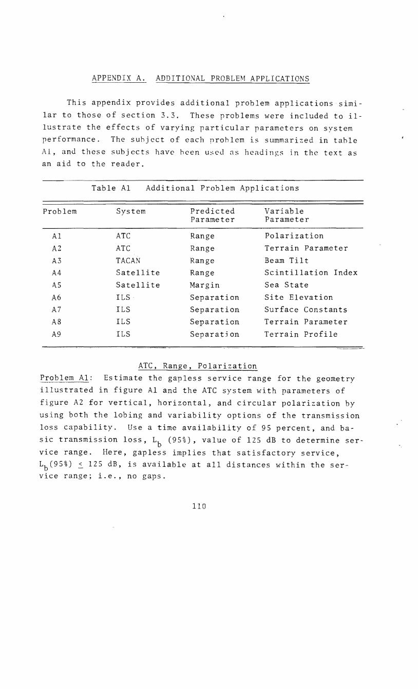
APPENDIX A. ADDITIONAL PROBLEM APPLICATIONS
This appendix provides additional problem applications simi
lar to those of section 3.3. These problems were included toil
lustrate the effects of varying particular parameters on system
performance. The subject of each problem is summarized in table
Al, and these subjects have been used ns headings in the text as an aid to the reader.
Problem
Al
A2
A3
A4
1\5
A6
A7
A8
A9
Table Al Additional Problem Applications
System
ATC
ATC
TACAN
Satellite
Satellite
ILS
ILS
ILS
ILS
Predicted Parameter
Range
Range
Range
Range
Margin
Separation
Separation
Separation
Separatjon
ATC, Range, Polarization
Variable Parameter
Polarization
Terrain Parameter
Beam Tilt
Scintillation Index
Sea State
Site Elevation
Surface Constants
Terrain Parameter
Terrain Profile
Problem Al: timate the gapless service range for the geometry
illustrated in figure Al and the ATC system with parameters of
figure A2 for vertical, horizontal, and circular polarization by
using both the lobing and variability options of the transmission
loss capability. Use a time availability of 95 percent, and ba
sic transmission loss, Lb (95%), value of 125 dB to determine ser
vice range. Here, gapless implies that satisfactory service,
Lb(95%) ~ 125 dB, is available at all distances within the service range; i.e., no gaps.
110
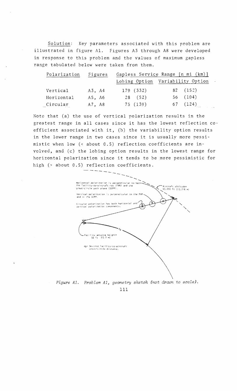
Solution: Key parameters associated with this problem are
illustrated in figure Al. Figures A3 through A8 were developed
in response to this problem and the values of maximum gapless
range tabulated below were taken from them.
Polarization Figures Gapless Service Range [n mi (km)]
Lobing Option Variability Option
Vertical A3,
Horizontal AS, Circular A7,
A4 A6 A8
179 (332)
28 (52)
75 (139)
82 (15 2)
56 (104)
67 (124)
Note that (a) the use of vertical polarization results in the
greatest range in all cases since it has the lowest reflection co
efficient associated with it, (b) the variability option results
in the lower range in two cases since it is usually more pessi
mistic when low (< about 0.5) reflection coefficients are in
volved, and (c) the lobing option results in the lowest range for
horizontal polarization since it tends to be more pessimistic for
high (> about 0.5) reflection coefficients. --- -- -- ----Horizontal polarizatiOr' is perpendicular to both..........._::--.......
thE' '.ac!lity-to~airc,.aft ray (FAR) and tht! ~~Aircraft altitudee: 9redt-c:rcle path plane (GCPP) ' 4'" 000 f (I 7 6
Veftica! po',aritat:on :c, p~rpend
and in t",e GCPP,
Circular polarizatior' has ooth horizm,~al and'
vert i cd: polar i zat i OP C~JI"HI)Onen~s.
Faci I i tv antenna height"' 50 f t (15. 2 m)
UU"' De,irec facility-to-aircraft q<cco{-clrcle distunc~.:.
'- ). t 3. I m)
'- ......
Figure Al. Problem Al~ geometry sketch (not drawn to scale).
111

PARAMETERS FOR ITS PROPAGATION MODEL IF-77 77/07/13. 22.15.49. RUN
BASIC TRANSMISSION LOSS FOR ATC
§~~~!~!~~!!2~-~g~f~~ AIRCRAFT (OR HIGHER) ANTENNA ALTITUDE: FACILITY (OR LOWER ANTENNA HEIGHT:
45000. FT (l3716.M} ABOVE MSL 50.0 FT (l5.2M) ABOVE FSS
FREQUENCY: 125. MHZ
SPECIFICATION OPTIONAL
AIRCRAFT ANTENNA TYPE: ISOTROPIC POLARIZATION: HORIZONTAL
EFFECTIVE REFLECTION SURFACE ELEVATION ABOVE MSL: GAIN SUM OF MAIN BEAMS: 0.0 OBI FACILITY ANTENNA TYPE: ISOTROPIC
POLARIZATION: HORIZONTAL
0. FT (O.M)
HORIZON OBSTACLE DISTANCE: 8.69 N MI (16.09KM) FROM FACILITY* ELEVATION ANGLE: -0/ 6/30 DEG/MIN/SEC ABOVE HORIZONTAL* HEIGHT: 0. FT (O.M} ABOVE MSL
REFRACTIVITY: EFFECTIVE EARTH RADIUS: 4586. N MI (8493.KM)* MINIMUM MONTHLY MEAN: 301. N-UNITS AT SEA LEVEL
SURFACE REFLECTION LOBING: CONTRIBUTES TO VARIABILITY SURFACE TYPE: AVERAGE GROUND TERRAIN ELEVATION AT SITE: 0. FT (O.N) ABOVE MSL TERRAIN PARAMETER: 0. FT (O.M) TIME AVAILABILITY: FOR INSTANTANEOUS LEVELS EXCEEDED
* COMPUTED VALUE
Notes: 1) Polarization, surface reflection lobing option and terrain parameter used for figures A3 through A8 and AlO and All vary as indicated in the figure captions.
2) Parameter values (or options} not indicated are taken as the assumed values (or options) provided on the general parameter specification sheet (table 2).
3) To simulate computer output, only upper case letters are used. Dual units are not provided on actual computer output.
Figure A2. ~oblems A1 and A2~ parameter sheet~ ATC.
112

p 1-' (.rl
R~a Ctdt 77/07/19. II. 3,.42
VERTICAL WITH LOBIN' ··············• F"ru IPUt F"rt~t~o~tU~ 125. ""' '•ia 0. 0 d9i r~,~,,,, 51. HI SO. It (15.2m)fss S•etth t•rth [•lddltl S01. H2 4SOOO. It (13716 .m)ms1 Pet•riutlea V•rt iul !IIWtrl 951.
Distance in km
90 I 100 200 300 4QO 5QO 600 720 I
CD -g
.::: -41" 41"
:~ I
..... ~ l t-.......
l I .....
~ l ~ .......... ·~ ' ~-· ~ .. ·-.... ...... .
100
110
120
150 0 -.::: 0 ·-41"
"" ·~·· ..•. . ...... t
~ !'\
" l'\\ 140
ISO ... -• \\ '"'
,,0 M c 0 &..
1-
\~ " ~ \" 1'--- ~
[--.... I
170
180
' --~ i'... ' I 190 1--......_
~ I 200
0 25 50 75 100 125 150 175 200 225 250 275 no 525 5! 0 3 5 .tO 210
OJstaftce ift ft Mi
Figure A3. T1•ansmission loss~ ATC~ vertical polarization~ tobing option. Transmission toss values were computed with parameters in figure A2 except for polarization and tobing option.
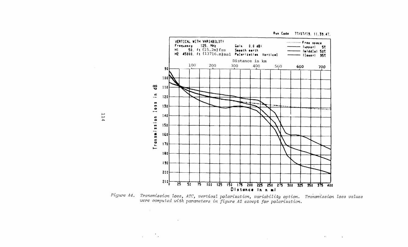
~
~ .j::o.
R11r. Ctdt 77107/19. 11.59.47.
VERTICAL WITH YARlABlLJT¥ ··············· Frtt spoct F"rt111UCy 125. l'tHz leoir. D. 0 dB; l~&,trl 51. HI 50. It (15.2m}fss S•ttth urth l•lddltl 501. H2 45000. It Cl3716.m)msl Ptlorizetitt Vtttictl ,, .. .,, 951.
Distance in km 100 200 300 400 sco 600 700 ,,___ 90
cO "0
iC -"" "" 0 -iC 0 ·-"" "" -• "" iC a ....
1--
I~ ,~ ...
~~--h-I !'I. to--..
'-........... ...... ~ ....... ~·· ~-· ............. ........
~ ... ···~ .........
~ ~ '\ l'\\ ~ l~ \~ ............
"" I
\~ i'-r-..... '"""" I
!DO
II 0
120
130
lAO
ISO
••o 170
180
19 ' --.. ~ ~ I
r---~ ' ~ ' 2C
21 'o 25 sc 75 100 125 150 115 2DD 225 250 275 soo 525 550 '~ 40 0 Oistaftct 1ft ft •i
Figure A4. TPansmission loss~ ATC~ vertical polarization~ VaPiability option. Transmission loss values were computed with parameters in figure A2 except for polarization.
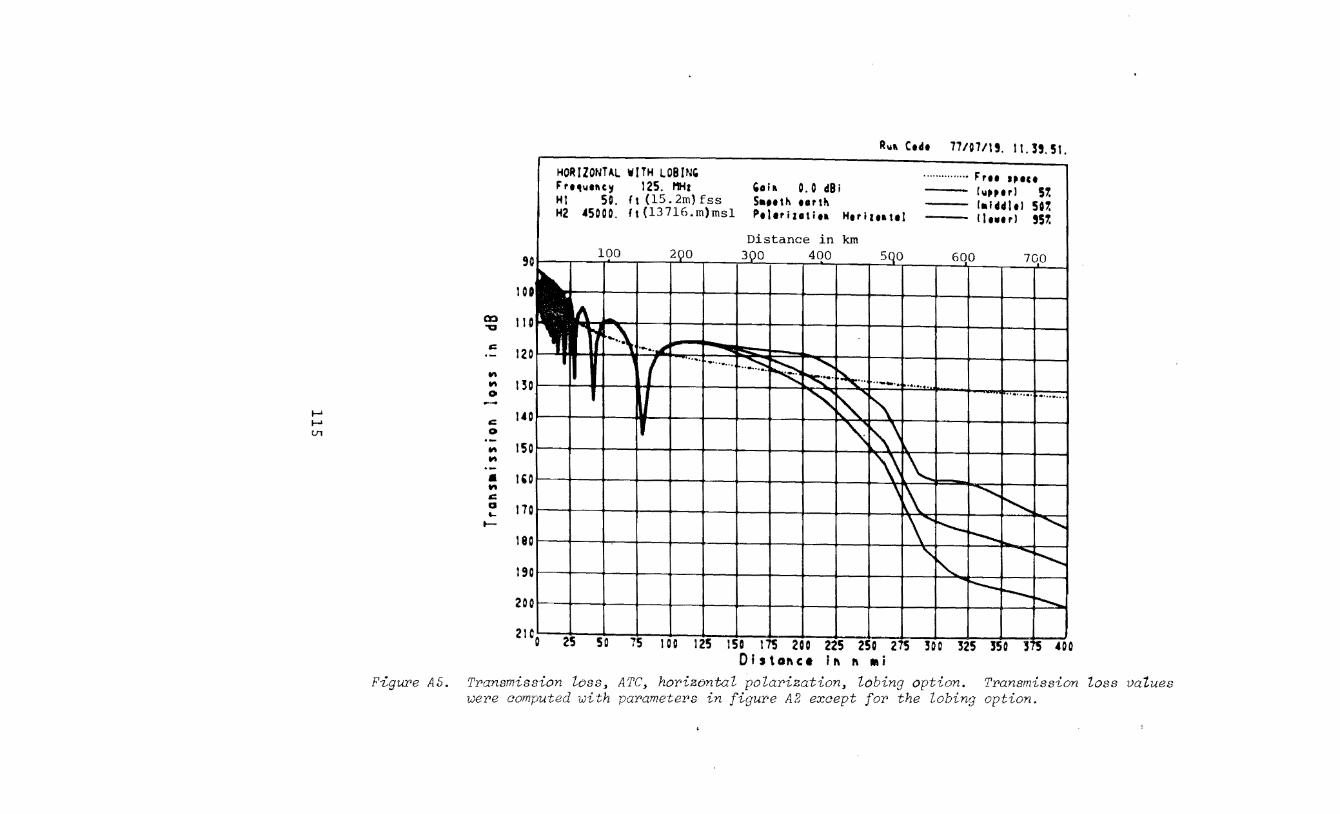
......
...... U1
R~• Ctdt 7710711!. 11.3!.51. --
HORIZONTAL WITH LOBIN' ............... Fru JPIIct FrtiJI4tU~ 125. P'IHt ,.i. 0.0 cl8i r~pperl 51. HI 50. ft (15. 2m) fss Sattth urth lalddltl 501. H2 .tSOOO. ft {137l6.m)ms1 Ptltr i tot ita Heriteatel lltwtrl !51.
Distance in km
' I 100 2QO 3_QO 400 SQO 600 700
I 0 I
(X) II "'CJ
.: 12
II\
15 II\
I 1... ~
~\ ) ·• .. J
1 I ..... •···•··· .. :::::;
~ ...........
) ~· ~ .. ··--~. ·•·•· . 0 -l.t .:
0 ·- 15 II\ II\ -• IG
" .•...•.
···~··· •1
~ i'\ 0
'\ l\\ 0
~ ~ 0 "' .: 0 17 ~
....... 18
\~ ........... ~ 0
\' 1'- """' 0 !'-..... I
' --~~ ~ I " r---1--~ I 20
• 'o 25 so 75 100 125 lSD 175 2Ga 225 250 275 !OD 325 550 1 r5 .tO 0 21
Oistol\ce II\ 1\ Mi
Figure AS. TPansmission loss, ATC, hoPizontal polarization, lobing option. TPansmission loss values wePe computed with paPameters in figure A2 except for the lobing option.
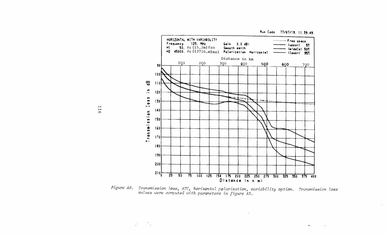
j--1 j--1
cr.
m 'V
a=
.. .. 0
a= 0 -.. .. -• .. a= a L-
t-
Rwft Ctdt 77/07/1,, 11.1,.4,.
HORIZONTAL WITH VARIABILITY ............... ,, ... ,.u Frt<twtacy 125. 11Hz Goia 0.0 d8i fll,ff J 51. Hl 50. ft (15.2m)fss Sauth ttrth la144ltl 501. H2 45000. ft (l37l6.m)msl Pel•ritttita Her i ua to I llt•trl !51.
Distance in km
I 90 lQO 200 3QO ~0 5QO 6QO 7QO
l.t
15
I~ 0 ~ I~ '""" -- ........_
~ r--r--.. ~
'""" -.... ~ -~ ~ .. r-- ~··· ··--·· ·•······ -- ......
~ ~ ..•...•. ...........
1'\ I
"\ L\\ I
1 0 0
11 0
120
1 50
1& I \\ \.. 17
\ ~· --.... ['.... 0
18 \' i'-.. ..............
!--...... 0
19 ' -~ "" 0
r-- r--. ~ ) 20
L - - 75 300 325 350 ' 5
40 21
50 5 1 DO 125 ISO 175 200 225 250 2 0 Distance inn mi
FiguPe A6. TPansmission loss~ ATC~ hoPizontal polaPization~ vaPiability option. TPanamiasion loss values wePe computed with parametePs in figuPe A2.
..,

Rwa Ctdt 77/07/19. 11.19.5•.
CIRCULAR VITH LOBIN' ··············· F'ree tll•ct F're•weuy 125. P'liz ,.;, 0. 0 d8i lwll!ltrl 51. HI 50. ft (15. 2m)fss Sattth .. rth lalddltl 501. H2 •sooo. ft ll37l6.m)msl Pe!triutlea Ci rcwltr I ltwtrl S$1.
Distance in krn
90 100 200 3QO 4QO 5QO 600 700,
:~ ~· :-.......... I v ....... .... -.. ·~ ~ ' I ~· ~·· ··- ........
~ ~~ ~ ·~·~···~ ····•·••j
I
'\ l'\\ I
\\ "' I
'~ .......... ~
\~ j'-...... 1"-- "
IOD
liD
120
150
1'0
150
I'D
170
180
·' -~ l'.. 190 r--. r--~ 200
21 10 25 so 75 100 125 HO lr! 200 225 2 0 vs 300 325 5! 0 1 rs •o 0 Olstaftce 1ft "al
Figure A?. Transmission loss~ ATC~ lo~ polarization~ Zobing option. Transmission loss values were oompu with parameters in figure A2 except for polarization and lobing option.
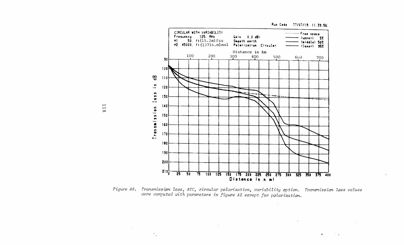
1-' 1-' 00
R,." Ctdt 77107/". II. 39.5,,
C!RCVLAR W)TH VAR!AB!LITY ............... F'ru .,.CI F'rt116111C!f 125. MHr bllill o. o dB i r,.,.,l St H1 50. ft(l5.2m)fss S•••th unh !•iddltl Sot H2 45000. It (13716.m)msl Ptleriutitll Ci rc,.Jer llturl 95t
Distance in km 100 290 300 4~0 500 600 700 I 90
co '0
..:: -"" "" 0 -..:: 0 ·-""
I!IJ...
I~ ~ " ~ r' r--
to--. r-- ....._ '
~ ~ -~ .. r-... ~ .... ··-..... ·····•· --
"' 1'\ •···•· .. ~ ..•... ~ '\ :'\\
100
11 0
120
150
t•o
150 "" -• \\ ~ I 1£0 "" ..:: 0 .... ..__
'[\ ""' ~ I
\~ ~ r--. ............
I
170
180
19 ' -~ I'. I
r--r--. t"'---... I 20
'o 25 so 15 100 125 l! 0 t'S 200 225 21 0 215 5DO m " o r'5 •• 21
0 Clttaftce II\ " •I
Figure AB. T~ansmiss1~n loss~ ATC~ ci~cular pola~ization~ va~iability option. T~ansmission loss values ZJe~e computed with pa~amete~s in figure A2 except fo~ pola~ization.

ATC, Range, Terrain Parameter
Problem A2: Estimate the maximum gapless service range for an
ATC system with the geometry illustrated by figure A9 and the
parameters of figure A2 with vertical polarization for smooth
earth, rolling hills, and mountains by using the transmission
loss capability with the variability option. Use a time availa
bility of 95 percent and basic transmission losses of 130 and
150 dB.
Solution: Pigures A4, AlO and All are applicable to this
problem and the values of gapless range tabulated below were ta
ken .from them. The increase in service range with terrain irreg
ularity for Lb(95%) = 130 dB is caused by a decrease in the specu
lar reflection coefficient as sur ce roughness increases, while
the decrease for Lb(95%) = 150 dB is caused by a decrease in radio
horizon distance. Except for the last case (mountains, 150 dB)
increasing irregularity tends to increase the service range be
cause of a corresponding decrease in reflection coe cient. In
the last case the decrease of service range occurs because of a
decrease in radio horizon distance. --------
Facility antenna 50 f t ( 1 5. 2 m)
--- ---....-.....-.... -
--------
Surface roughness computed from ~h is used in the calculation of reflection coefficients.
dD= Desired fac iIi ty- to-aircraft great-circle distance.
...... (
Aircraft altitude= 45.000 ft 113,716 m)
...... -........ .........
.........
' ..........
' ' ' ' ' -- ___ ......._ 0 ' ----- " ,/" I ......_
,/ I ' I
/ I / I
\ ' I '. ..... ,/ I
I
Facility horizon parameters are computed using the terrain parameter,~h. Beyond this horizon the earth is considered smooth.
Figure A9. Problem A2~ geomd-l'U ._,7<.etah (not draum to saale). 119
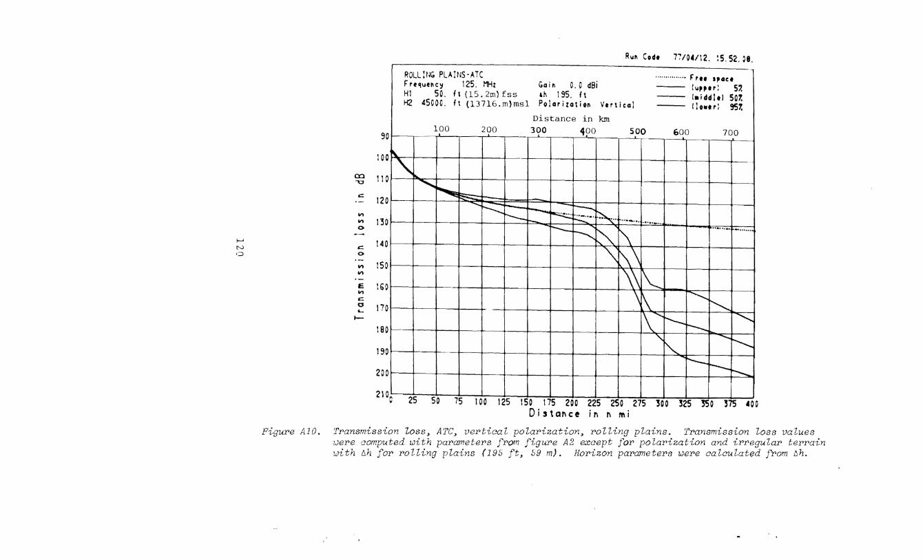
1-' N <:::)
Ru~ Codt 77/0./12. 15.52. ~8.
ROLL!tJG PLAINS-ATC ............... F'rtt lfiCICI F requertc~ 125. MHz Gai11 0. 0 dBi (upptrl 51. Hl 50. ft (l5.2m) fss Ah 195. ft l•iddltl 507. H2 45000. ft (l37l6.m)msl Polarization Vertical tlo11trl 957.
Distance in km
9 100 200 300 100 500 600 700 )-··
~
10
en 11 -o
1\.
~" I!.. ........... ~ c:
12 V\
13 V\ 0 --
14 c: 0
·- 15 V\
I -r-::: -r--.. !'-- -~ r=.:.::··· ~· '- ............ ·····-·· I ..__ ..........
-··~ ...... r---... ~ [\ I
'\ [\\ I
V\
-e. 16 I \\ 1\_ V\ c: 0 ..._
1--
IS
\ l\ ~ ~ I
1\-1'-r--... ~ I
" ......... ~ ~ I 19
r--r-- r-.... I 20
J \ 21 ·c 25 50 75 I 00 125 ISO 175 200 225 250 275 '500 325 '550 '575 •oo
Distance in n mi
Figure AlO. Transmission loss, ATC~ vertical polarization~ rolling plains. Transmission loss values were computed with parameters from figure A2 except for polarization and irregular terrain with 6h for rolling plains (195ft, 59 rn). Horizon parameters were calculated from 6h.
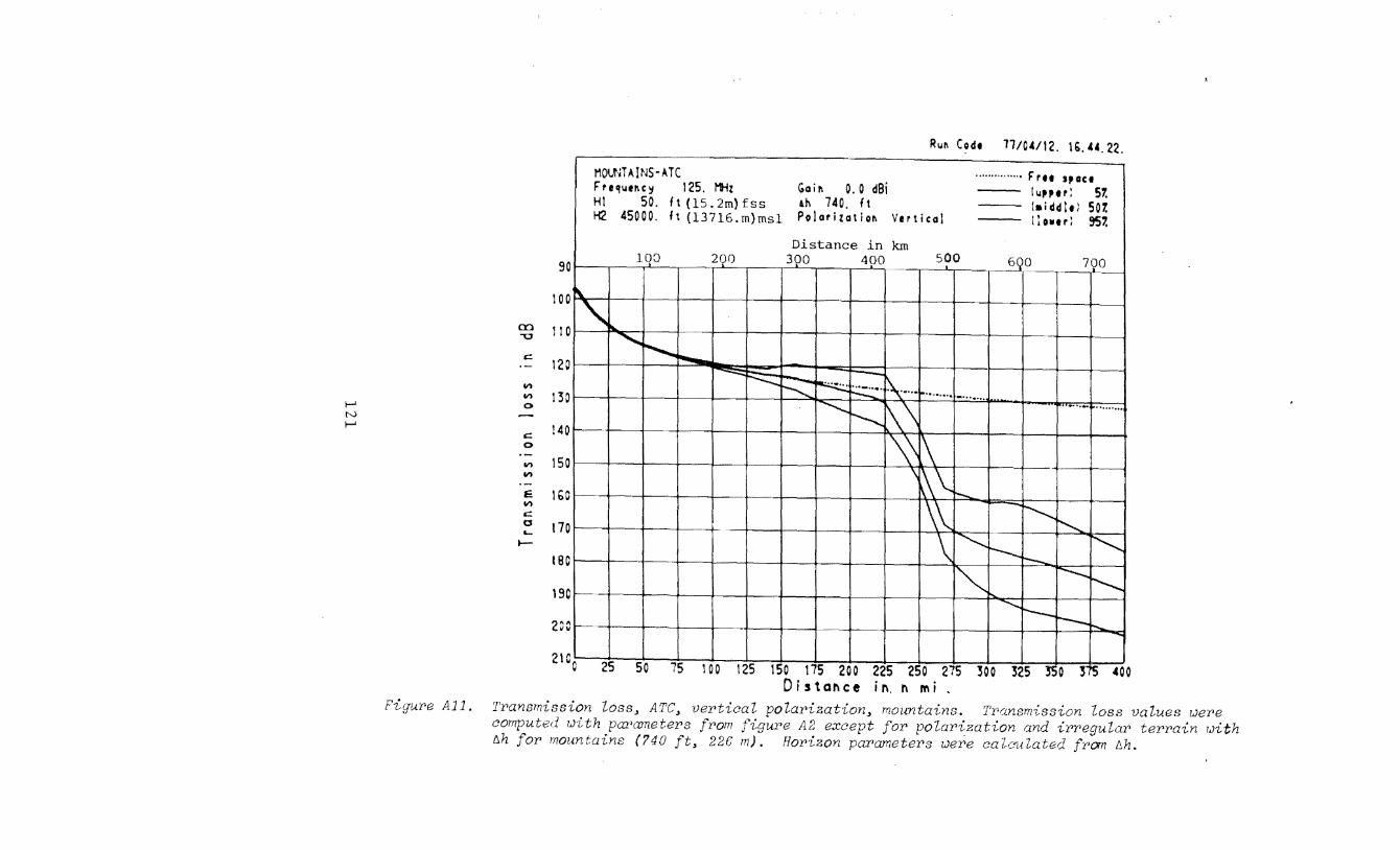
1-' N 1-'
Ru~ Codt 1110•112. 1&.••.22.
MOUNTAINS-ATC ............... F rtt ,,OCt F',. ql.ltll c ~ 125. l'tiz Gai11 0. 0 dBi 1~.~,.,: 57. HI 50. ft (15. 2m) fss lh 740. ft l•iddlt) 507. H2 45000. ft (l3716.m)msl Polarizatioll Vertical llo .. r: 957.
Distance in km 100 200 300 400 500 6QO 700 r·-•--90
ro -o
c:
)~
~ i
...........
) ~ -......
I 00
II 0
120 ..., ..., 0
c: 0 -..., ..., -e. ..., c: Cl ....
I--
!40
-~ ~ ~ ~-· '\···· ~ ........ J -·····--.............. L\\ ····- ........... ~ J
~ l\ I 0 I
\~\ c r-...
\\ ~ ~ 0
\ '-.....,
"" 1---0 ~
130
ISO
1&0
170
19
I~ --. ~ o~--\9
-....... ..___ 1--r--... : 2~
I
'-21 25 so 75 too 125 tso 175 200 225 2so 275 3oo 325 3So 375 •oo
D i s tal'\ c e in. n M i . Fi(JI--tre A11. Transmission loss~ A1'C~ vertical polarization~ mountains. 1'rl1nsm-ission loss values 1.Jere
computed with pcn•ameters from figure A2 except for polarization and irregular terrain 7Jith M for mountains (740 ft~ 226 m). Horizon parameters wePe calculated fNJm t:.h.
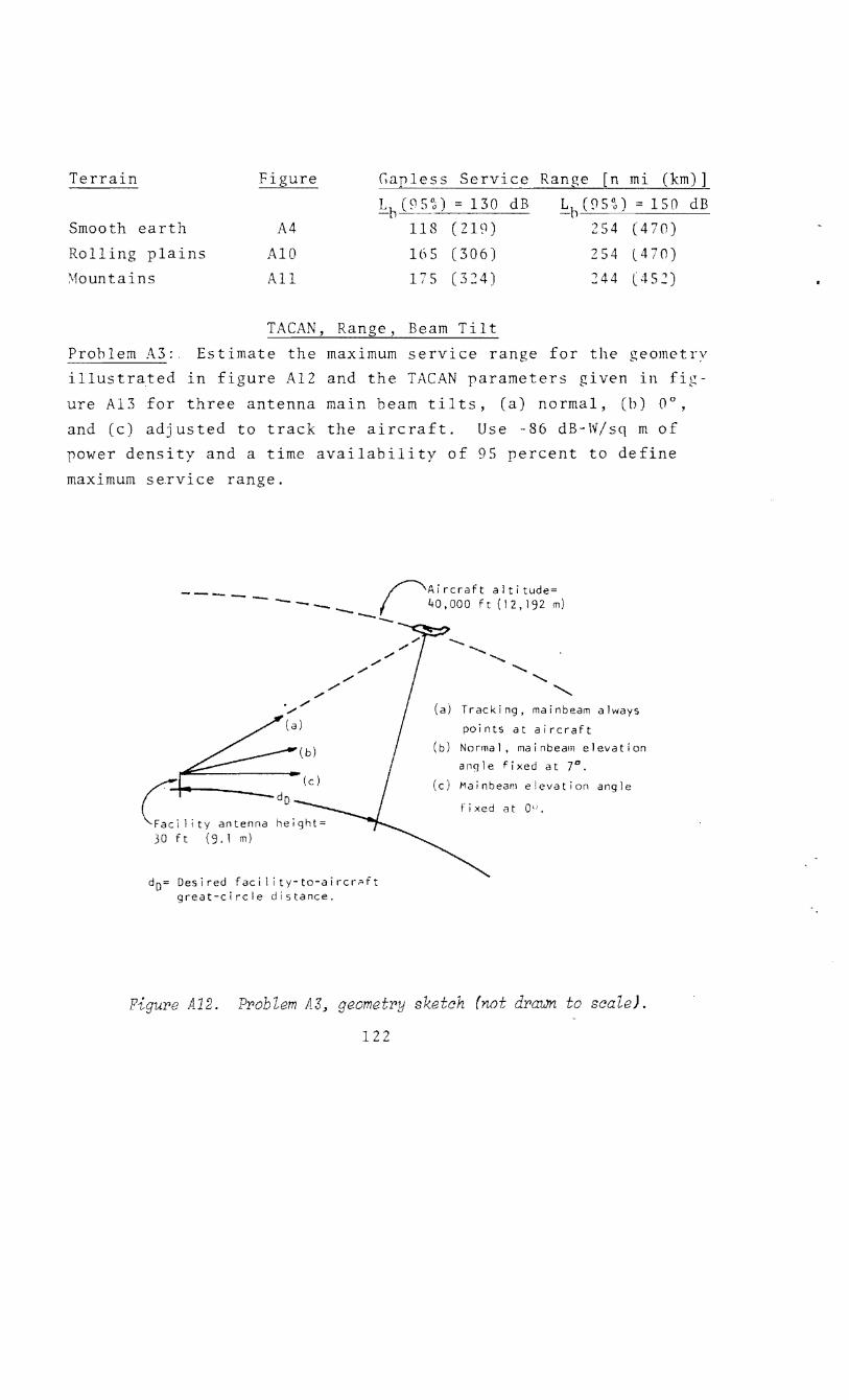
Terrain Fi e Gar less Service Ran~e [n mi (km)]
130 dB 150 dB Smooth earth A4 118 (219) 254 (470)
Rolling plains AlO 165 (306) 254 l470) :.1ountains All 175 (324) 244 ( 4 52)
TACAN Beam Tilt
Problem A3: Estimate the maximum service range for the geometry
illustrated in figure Al2 and the TACAN parameters given in fi~
ure Al3 for three antenna main beam tilts, (a) normal, (b) 0°,
and (c) adjusted to track the aircraft. Use -86 dB-W/sq m of
power density and a time availability of 95 percent to define
maximum service range.
----- rAircraft altitude= --- 40,000 ft (12,192 m) ---
do= Desired faci 1 ity-to-aircr~ft great-circle distance.
........... ....................
.......... ..........
'-.... (a) Tracking, mainbeam always
points at aircraft
(b) Normal, mainbeam elevation
anqle fixed at 7°. (c) Mainbeam elevation angle
fixed at ou.
FiguPe A12. Problem A3~ geometPy sketch (not dPa~ to scale).
122
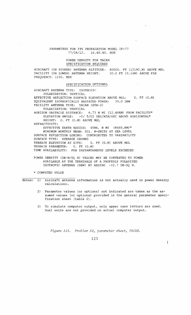
PARAMETERS FOR ITS PROPAGATION MODEL IF-77 77/04/12. 16.48.40. RUN
POWER DENSITY FOR TACAN
§~~~!~!~~~!~~-~Q~!~~ AIRCRAFT (OR HIGHER) ANTENNA ALTITUDE: FACILITY (OR LOWER) ANTENNA HEIGHT:
40000. FT (12192.M) ABOVE MSL 30.0 FT (9.14M) ABOVE FSS
FREQUENCY: 1150. MHZ
SPECIFICATION OPTIONAL
AIRCRAFT ANTENNA TYPE: ISOTROPIC POLARIZATION: VERTICAL
EFFECTIVE REFLECTION SURFACE ELEVATION ABOVE MSL: 0. FT (O.M) EQUIVALENT ISOTROPICALLY RADIATED POWER: 39.0 DBW FACILITY ANTENNA TYPE: TACAN (RTA-2)
POLARIZATION: VERTICAL HORIZON OBSTACLE DISTANCE: 6.73 N MI (12.46KM) FROM FACILITY*
ELEVATION ANGLE: -0/ 5/02 DEG/MIN/SEC ABOVE HORIZONTAL* HEIGHT: 0. FT (O.M) ABOVE MSL
REFRACTIVITY: EFFECTIVE EARTH RADIUS: 4586. N MI (8493.KM)* MINIMUM MONTHLY MEAN: 301. N-UNITS AT SEA LEVEL
SURFACE REFLECTION LOBING: CONTRIBUTES TO VARIABILITY SURFACE TYPE: AVERAGE GROUND TERRAIN ELEVATION AT SITE: 0. FT (O.M) ABOVE MSL TERRAIN PARAMETER: 0. FT (O.M) TIME AVAILABILITY: FOR INSTANTANEOUS LEVELS EXCEEDED
POWER DENSITY (DB-W/SQ M) VALUES MAY BE CONVERTED TO POWER AVAILABLE AT THE TERMINALS OF A PROPERLY POLARIZED ISOTROPIC ANTENNA (DBW) BY ADDING -22.7 DB-SQ M.
* COMPUTED VALUE
Notes: 1) Aircraft antenna information is not actually used in power density calculations.
2) Parameter values (or options) not indicated are taken as the as-sumed values (or options) provided in the parameter speci-fication sheet (table 2).
3) To simulate computer output, only upper case letters are used. Dual units are not provided on actual computer output.
Figure A13. A 3.. parameter TACAN.
123
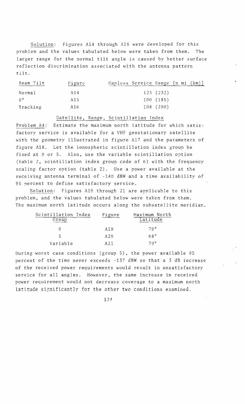
Solution: Figures Al4 through Al6 were developed for this
problem and the values tabulated below were taken from them. The
larger range for the normal tilt angle is caused by better surface
reflection discrimination associated with the antenna pattern
tilt.
Beam Tilt Figure Gap less Service Range [n ml (km)]
Normal Al4 125 (232) oo Al5 100 (185)
Tracking Al6 108 (200)
Satellite, Range, Scintillation Index
Problem A4: Estimate the maximum north latitude for which satis-
factory service is available r a VHF geostationary satellite
with the geometry illustrated in figure Al7 and the parameters of
figure Al8. Let the ionospheric scintillation index group be
fixed at 0 or 5. Also, use the variable scintillation option
(table 2, scintillation index group code of 6) with the frequency
scaling factor option (table 2). Use a power available at the
receiving antenna terminal of -140 dBW and a time availability of
95 percent to define satisfactory service.
Solution: Figures Al9 through 21 are applicable to this
problem, and the values tabulated below were taken from them.
The maximum north latitude occurs along the subsatellite meridian.
0
5
Variable
Al9
A20
A21
Maximum North Latitude
During worst case conditions (group 5), the power available 95
percent of the time never exceeds -137 dBW so that a 3 dB increase
of the received power requirements would result in unsatisfactory
service for all angles. However, the same increase in received power requirement would not decrease coverage to a maximum north
latitude significantly for the other two conditions examined.

........ N U"1
P.ur. Code 11/0.C/12. "· .CB . .CO.
HAIN LOBE AT NORMAL ELEVATION .............. , F'ru IJIGCI F'requer.c~ 1150. MHz . EIRP 39. 0 d81t luJIJI tr I 57. HI 30. ft (9.lm)fss S111ooth earth l•iddltl 507. H2 40000. ft (12192.m)msl Polar i zat ior. Vertical llowtrl ~?.
Distance in km
-bO 5Q lClO 1~0 2DO 2?0 300 350 400 4_{0 5QO 550 I
E. -70
cr II'\
......... 3 -80
I
a:l "\::)
-90 ~
-::r-. -I 00 -II'\
c -110
lL\. - - l lL'\7' ........... IY" ~
~ I I
~ ~ I I --~ """--.. ~ ---.
~-........._ ~ .. ····-····-·· ······· I
~ r--- ---~ \ -D\ 1\ ... ""0
,_ -120 \ \~ 4.1 :a 0
-130 Q... 1\\ ~
-140 \" ~! -150 \
~ i -- --I bOO
25 so 75 I 00 \25 \SO 175 200 225 250 275 300 0 i stance in 1'1 rni
Figure A14. Power densit;t, TACAN, main lobe at normal elevation angle. POtJer density values I,,epe eomputed with the parameters from figure A 13.
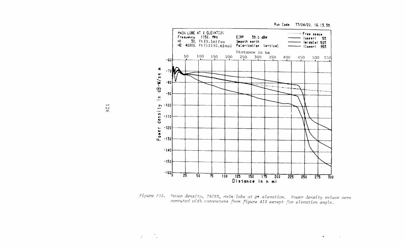
f-A N 0\
£
o· VI
........ Jll
I en -u
c
-GO
-70
-80 I
-90 J
~ -too ) -VI
) c -110 .., -u
.... • \20 .., ll 0
a... -1'50
- t4 I
-15 I
1'1 ·1 '·o
R1111 Code 7?/04/20. I G. 1'5. '53.
MAIN LOBE AT 0 ELEVAT!O:; ····· ········· F'ru space Frt~lltiiC!f 1150. l'tiz E:RP '59.0 dSW t~&pptr) 57. HI '50. h (9.1m)fss S.ooth urth l•iddltl 507. H2 40000. ft (l2192.m)msl Po:arizotioll 'itrtical !lower) 957.
Distance in km 50 100 150 200 2~0 300 350 400 4'30 500 5SG
/},. rr ~ --t--- r-- --!'--... 1'---. r---......_ -... ~ ·~· ~
............. ,,
1---......... _.
1--- t-- ·•·····•····· .............. ....... 1-- ~\' r---
\' l\ \\" ~ l\_~ \ ~
'\ ~
' 25 so 75 100 125 150 t75 200 --225 -250 ---21'5 '500
Distance in n mi
Fif1Ur>e l'.l ,s. Po1.JeY' dens i. t.'l, TAr'AN, f11ain lobe at oo elevation. Power• density vo lues ?;Je:re comvuted h'lth 1Y<I'Ofl1eteY's f'Y'om [1:guY'e A1.1 f'o:r elevation angle.
~"II :odt 17101/U. ll. 03. H.
TAC~N TRACK JN; ··········F'•u HOCI r., 1 .. tt~cy 115 D. 11Ht [JRP 39.0 d8W I"H"I 52 HI 3D. f\(9.lm)fss S•oo th tot\~. l•iddltJ 501. H2 40000. fl (12192.m}msl Polori:otioll Vtrtical lion•' 957.
Distance in km
e
50 100 150 200 250 3QO _3~() 400 4/0 soo sse I ---..1 I ..L ··- - __.1_
' "-... 1·-
_,0
·70 cr ....
........ :a • en
-c:;,
,;::
·-1-' 7'\
~ r---. - r---r---1----·-
""" -~ ··-\· 1'--- ~ "··-......... ............. .............. ....._ t---.. It-- ·-·--1--- r--- ~~' r---,..... 1-- ------- ----
·80
·90
·UO N --..,_]
"' ,;:: I \\ l\ 1--- -· -·-· -110 ...
"0
._ \ l\" "' ---120 ...
Jl 0
tL \"" ----- ···-·-·130
-14
I \ ~ l 1--··-- 1-
l '\ ~ I -------- ~-·15 ..........,
I
l . -·I &.0 25 50 75 100 125 ISO 175 200 225 275 250 300
Oistal\ce il\ 1\ mi
?ipure A16. ?m,,~'i' fens1~t71j TACMJj lobe tr•acking aircraft. Po7,Jer 1Jo.lues /,,ere eon~':<. . !.'1: th .figure A13 except .for trac'V.inp opHo-r:.
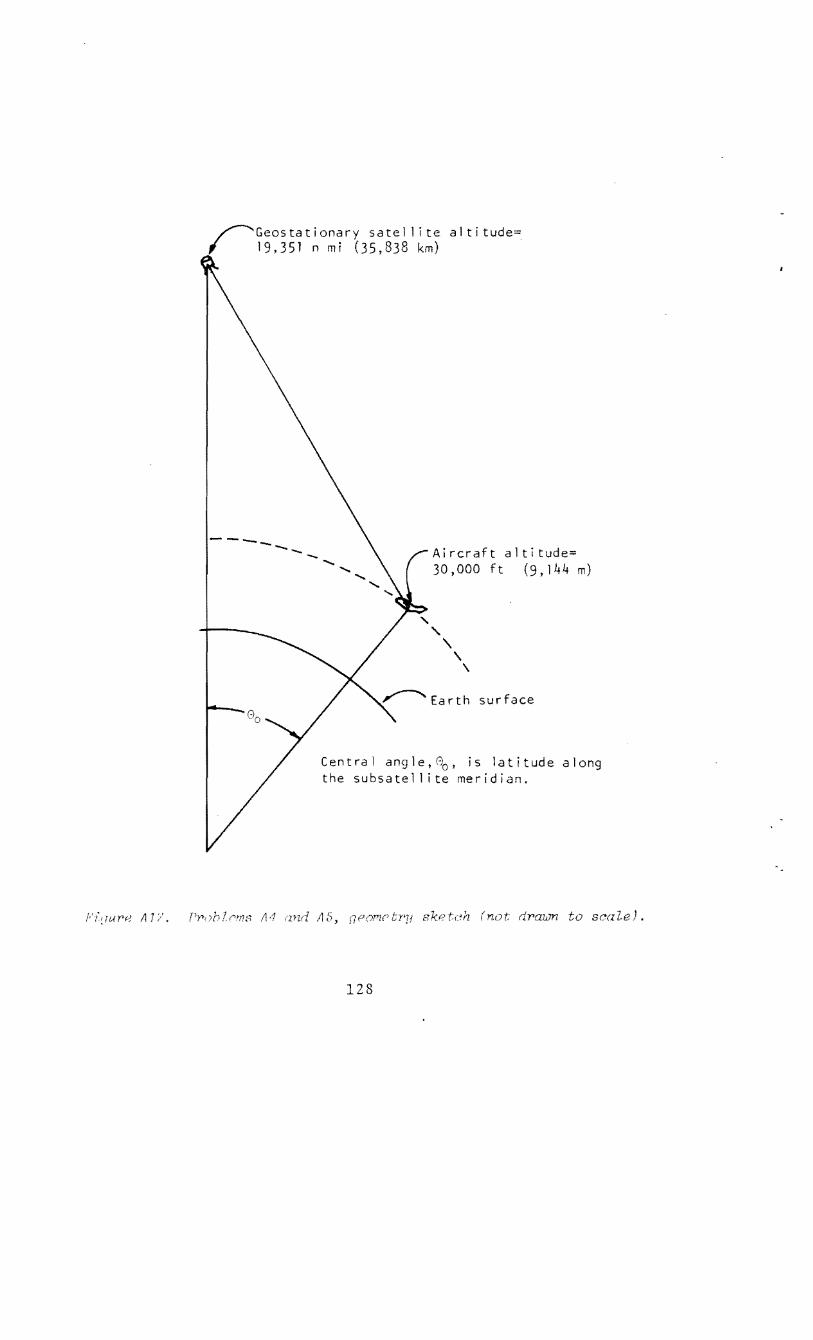
/Geostationary satellite altitude=. 19,351 n mi (35,838 km)
----...._ --- Aircraft altitude= 30,000 ft (9, 144m)
sur face
Central angle,80 , is latitude along the subsatel lite meridian.
128

PARAMETERS FOR ITS PROPAGATION MODEL IF-77 77/09/01. 17.42.47. RUN
POWER AVAILABLE FOR VHF SATELLITE SEA STATE 0
§~~~!~!~~!!2~-~Q~!~~ AIRCRAFT (OR HIGHER) ANTENNA ALTITUDE: 19351. N MI {35838.KM) ABOVE MSL FACILITY (OR LOWER) ANTENNA HEIGHT: 30000.0 FT (9144.M) ABOVE FSS FREQUENCY: 125. MHZ
SPECIFICATION OPTIONAL
AIRCRAFT ANTENNA TYPE: JTAC BEAMWIDTH, HALF-POWER: 10.00 DEGREES POLARIZATION: CIRCULAR TILT IS -90.0 DEGREES ABOVE HORIZONTAL
EFFECTIVE REFLECTION SURFACE ELEVATION ABOVE MSL: 0. FT (O.M) EIRP PLUS RECEIVING ANTENNA MAIN BEAM GAIN: 35.0 DBW FACILITY ANTENNA TYPE: JTAC
BEAMWIDTH, HALF-POWER: 20.00 DEGREES POLARIZATION: CIRCULAR ANTENNA IS TRACKING
HORIZON OBSTACLE DISTANCE: 208.85 N MI (385.79KM) FROM FACILITY* ELEVATION ANGLE: -2/49/36 DEG/MIN/SEC ABOVE HORIZONTAL* HEIGHT: 0. FT (O.KM) ABOVE MSL
IONOSPHERIC SCINTILLATION INDEX GROUP: 0 REFRACTIVITY:
EFFECTIVE EARTH RADIUS: 4586. N MI (8493.KM)* MINIMUM MONTHLY MEAN: 301. N-UNITS AT SEA LEVEL
SURFACE REFLECTION LOBING: CONTRIBUTES TO VARIABILITY . SURFACE TYPE: SEA WATER
STATE: 0 CALM {GLASSY) 0.00 FT (O.OOM) RMS WAVE HEIGHT
TEMPERATURE: 10. DEG CELSIUS 3.6 PERCENT SALINITY
TERRAIN AT ELEVATION SITE: 0. FT {O.M) ABOVE MSL TERRAIN PARAMETERS: 0. FT (O.M) TIME AVAILABILITY: FOR INSTANTANEOUS LEVELS EXCEEDED
* COMPUTED VALUE
Notes: 1) Parameter values (or options) not included are taken as the assumed values (or options) provided in the general parameter specification sheet (table 2) .
2) To simulate computer output, only upper case letters are used. Dual units are not provided on actual computer output.
Figure AlB. Problems A4 and AS~ parameter t~ VHF satellite.
129
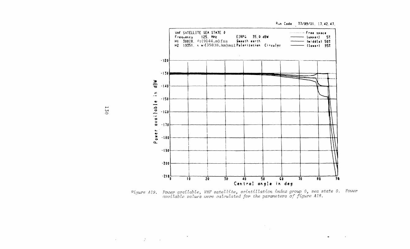
R~,~,. Code ll/09/01. 11 . .&2 . .&1.
VHF SATELLITE SEA ST~lE 0 ...... ··· i=ru HOCt F'rt11.1t!\Clf 125. ~: ElRPG 35.0d8W hillllttJ 57. HI 30000. f t ( 9144 .rn) fss Saooth eorth l•iddlel SO?. H2 19351. ~ llli{35838.km)rns1Poloritotior. Circul~r !lower I 957.
-120 -
-130
::. en -140 "e
·········~ ...... ~
~ - -150 t'-.
~ -i-' ..Q VI 0 ·I bO 0 -...
0 > 0 ·170 ... ~
ll . t 80 0
Q...
-130
-20~
l\ I \ J l
I : 1 I i
J l -2t00 30 lO 50 'O 10 20 80 10 9'
Central angle in deg
h'i({UY'e A 19. PmueY' available, VHF satell1: scintillation index gY'oup 0, sea state 0. available values /,JeY'e calculated for' the paY'ameteY's of figuY'e AlB.
PouJeY'
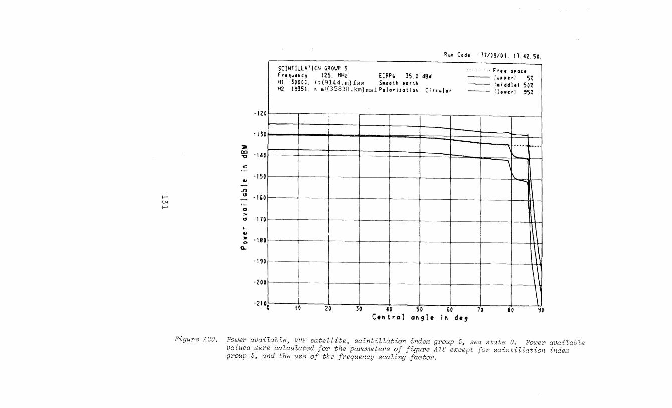
I-' tM I-'
Run Codt 77/09/01. 17.42. 50.
SCINT!LL~TICN GROvP S ....... "··Fret spact F rt~uncy 125. MH: EIRPC. 35. 0 dB'i :uppt ri 51. HI 30000. lt{9144.m)fss S•oo 111 earth '•iddltl 507. H2 19351. n 111i(35838.km)mslPolarization (irc~o~lar tlowtr! 951.
-·20 I
I ·130
]II CIC ~
\ ............ .... ) -140
c:: ' -"'
I !\ ..... ·150
-..0 0 -I 60 I
0 > 0 -170 I t...
"' :. ·18 0 k\ I
Q..
-I~ I t----· -
-20 I \ ' I i \ -21.0 I 0 20 30 40 50 60 70 80 90
Cerdral ar~gle ir~ deg
Figure A20. Power available~ VHF satellite~ scintillation index group 5~ sea state 0. Power available values were calculated for the parameters of figure A18 except for scintillation index group 5~ and the use of the frequency scaling factor.
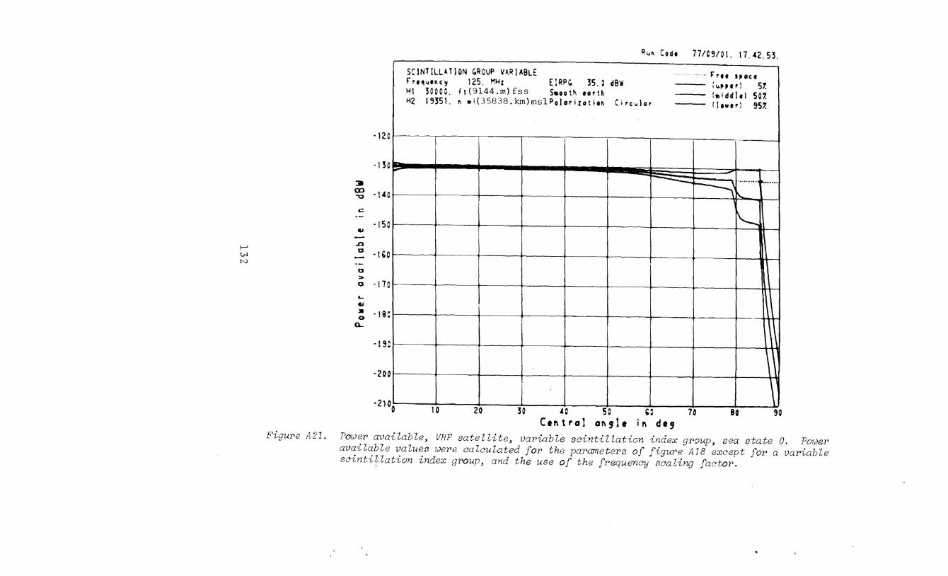
,__. c..N N
Rul\ Codt 71/09/0l. 17. 42. 53.
SCINllLLATION ~ROVP V'RIABLE ..... · ...... F'ret s,oct r a ""'uc ~ 125. MHz EIRP\0 35. 0 dBii :~.~,ul 57. HI 3COOC. f t (9144 .m) fss Saoo t 1'1 tor! II faiddltl 501. H2 19351. f\ llli(35838.km)mslPo!orizatio~ Circwlar flourl 951.
·12 0 I
I -- t:5 0
:ill co "0 ·14 --- .......... ; ......
~I\ I
c:: -·15 ~ I ., -Jl
0 - • I G 0 ·-0 > 0 -17 I
.... ., ll -19 0
a...
-19 ' \ '
-20 I \' , 30 .co so '~ 70
I 1 . - . -·21.0 10 20 80 90
Central angle in deg
Figu~e A21. Powe~ availableJ VHF satellite, va~iable scintillation index g~oup, sea state 0. Powe~ available values we~e calculated fo~ the pa~amete~s of fig~e AlB except fo~ a va~iable scinti?lation index g~oup, and the use of the f~equency scaling facto~.
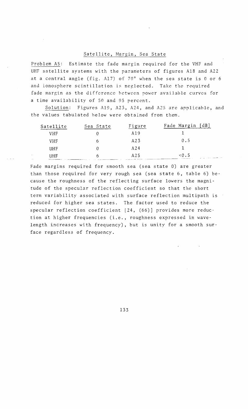
Satellite, Margin, Sea State
Problem AS: Estimate the fade margin required for the VHF and
UHF satellite systems with the para~eters of figures Al8 and A22
at a central angle (fig. Al7) of 70° when the sea state is 0 or 6
and ionosphere scintillation is neglected. Take the required
fade margin as the difference between power available curves for
a time availability of 50 and 95 percent.
Solution: Figures Al9, A23, A24, and A25 are applicable, and
the values tabulated below were obtained from them.
Satellite Sea State Fade Margin (dB]
VHF 0 Al9 1
VHF 6 A23 0.5
UHF 0 A24 1
UHF 6 A25 <0.5 ·~-----·
-·----·---·-~
Fade margins required for smooth sea (sea state O) are greater
than those required for very rough sea (sea state 6, table 6) be
cause the roughness of the reflecting surface lowers the magni
tude of the specular reflection coefficient so that the short
term variability associated with surface reflection multipath is
reduced for higher sea states. The factor used to reduce the
specular reflection coefficient [24, (66)] provides more reduc
tion at higher frequencies (i.e., roughness expressed in wave
length increases with frequency), but is unity for a smooth sur
face regardless of frequency.
133
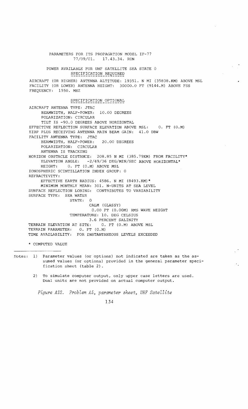
PARAMETERS FOR ITS PROPAGATION MODEL IF-77 77/09/01. 17.43.34. RUN
POWER AVAILABLE FOR UHF SATELLITE SEA STATE 0
~~~~!~!~~!!~~-~g~!~~ AIRCRAFT (OR HIGHER} ANTENNA ALTITUDE: 19351. N MI (35838.KM) ABOVE MSL FACILITY (OR LOWER) ANTENNA HEIGHT: 30000.0 FT (9144.M) ABOVE FSS FREQUENCY: 1550. MHZ
SPECIFICATION OPTIONAL
AIRCRAFT ANTENNA TYPE: JTAC BEAMWIDTH, HALF-POWER: 10.00 DEGREES POLARIZATION: CIRCULAR TILT IS -90.0 DEGREES ABOVE HORIZONTAL
EFFECTIVE REFLECTION SURFACE ELEVATION ABOVE MSL: 0. FT (O.M) EIRP PLUS RECEIVING ANTENNA MAIN BEAM GAIN: 41.0 DBW FACILITY ANTENNA TYPE: JTAC
BEAMWIDTH, HALF-POWER: 20.00 DEGREES POLARIZATION: CIRCULAR ANTENNA IS TRACKING
HORIZON OBSTACLE DISTANCE: 208.85 N MI (385.79KM) FROM FACILITY* ELEVATION ANGLE: -2/49/36 DEG/MIN/SEC ABOVE HORIZONTAL* HEIGHT: 0. FT (O.M) ABOVE MSL
IONOSPHERIC SCINTILLATION INDEX GROUP: 0 REFRACTIVITY:
EFFECTIVE EARTH RADIUS: 4586. N MI (8493.KM)* MINIMUM MONTHLY MEAN: 301. N-UNITS AT SEA LEVEL
SURFACE REFLECTION LOBING: CONTRIBUTES TO VARIABILITY SURFACE TYPE: SEA WATER
STATE: 0 CALM (GLASSY)
0.00 FT (O.OOM) RMS WAVE HEIGHT TEMPERATURE: 10. DEG CELSIUS
3.6 PERCENT SALINITY TERRAIN ELEVATION AT SITE: 0. FT (O.M) ABOVE MSL TERRAIN PARAMETER: 0. FT (O.M) TIME AVAILABILITY: FOR INSTANTANEOUS LEVELS EXCEEDED
* COMPUTED VALUE
tlotes: 1) Parameter values (or options) not indicated are taken as the assumed values (or options) provided in the general parameter specification sheet (table 2).
2) To simulate computer output, only upper case letters are used. Dual units are not provided on actual computer output.
PiguPe A22. FPobZem AS~ paPameter sheet~ UHF Satellite
134

, ...... lM V1
Figure A23.
-120
-1!0
:a 00 ·I AO "'Q
.,:; -
-150 ... -..0 0 -1&0 -·-0 > 0 -110 ,_ ... ! -18C
a..
·19C
-200
·210 0
Rw~ Codt 771:9/~1. 17.A3.3t.
VH~ SATELLITE SEA STAT£ & ~,~~~~~cy 125. M~r £IRP' 35.0 d8W HI !OOOC. lt(9144.m)fss Saootll tortll H2 19!51. ~ ai(35838.km)ms1Polorizotioll Circ~lor
............ ~ , .. ,,.,. :~,.,; 57. !aiddltl 507. n ... ,l '5'-
~···~·1'-·····
~
1 90 10 20 30 'C 50 GO 70 8Q
Cer\tral ol'\,le il"' de' Power> avaitab VHF satel values weJ'e calculated fo~
teJ scintillation index g~oup OJ sea state par•ameter>s of figur>e A18 except for sea
e. P01Jer• available state.
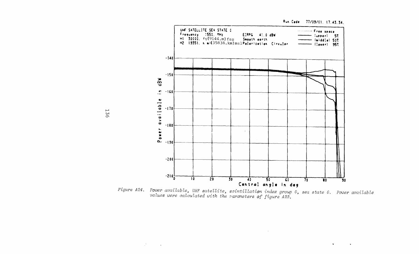
1-' (A (]\
:ill CD v
·l•o If--
·ISO
c: • '&0
"' .n 0 -{7 I
0 ::. 0 -1 e I ._
"' :II 0
0- ·19 I
·2 0 I
I ·21.0
R-.t. Ctdt 77109/Cl. 11. -'3. "5-'.
UHf SATELLITE SEA STATE C ............ r,., .,ou ~ 'flll-.tiiC\j :550. I'!Ht ElRPii ":.o d9w : .. ,.,, 57. 1-11 3000C. lt(9144.m)fss Sautil urtil [aiddltl 501. H2 19351. " ai(35838.km)ms1Pelt,izotiu Circ-.for 'l•••, l ~7.
" ~ ~
"" '
1 0 2D !0 U 50 GO 70 -. to 90 Ctr\tral Or\9lt ir\ dt9
Figure A24. Power available~ UHF satellite~ scintiUaticm index group o. sea state 0. Power avaiZaMe values were calculated zJith the r>a:t'ameters of figure A22.
~
lN '-1
Ruft Codt 77/09/01. 11.43.37.
VHf SATEL~JTE SEA STAlE & ............... F'ru spoct F' rt1YtiiC~ 1550. MHz EIRPCi 41. 0 dBW { YPPI rl 57. HI 30000. It (9144. m} fss Saootll urtl\ {aiddltl 507 H2 1335). 11 ai(35838.km)ms1Poloritoti011 C i rculor f1 owtrl 951.
I -140
.) r--'--:;. l
·ISO
co "0 ~ ole -... -- ~
·1&0
..0 a -110 -·-a > a r---180 ... ... :II 0
Q... lr---190
-200 0
I 1 --·21.0 30 4~ SO GO 70 80 90 I 0 20
Cer\tral Or\,le ir\ de'
Figu.rt: .. ; ·~s. PoweY' available, UHF satel Ute, scintillation index gY'oup 0, sea state 6. PoweP available values were calculated with paramete.ros from figure A22 except foY' sea state.
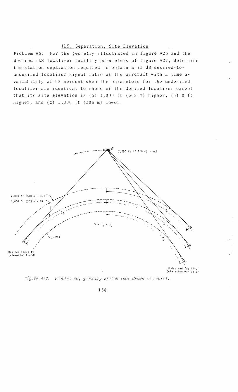
ILS, Separation, Site Elevation
Problem A6: For the geometry illustrated in gure A26 and the
desired ILS localizer facility parameters of figure A27, determine
the station separation required to obtain a 23 dB desired-to
undesired localizer signal ratio at the aircraft \vith a time a
vailability of 95 percent when the parameters for the undesired
locali:er are identical to those of the desired localizer except
that its site elevation is (a) 1,000 rt (305 rn) higher, (h) 0 ft
higher, and (c) 1,000 ft (305m) lower.
2,000 ft (610 m)- msl~ , ... ~
I ,000 ft (305 m)- m~~~.--"
/
/ /
/
/ /
/
/ /
/ /
/
Desired facility (elevation fixed)
/ /
/
.,.------ 7,250 ft (2,210 m) - msl
-----+--:---------------- ....... -
138
Undesired facility (elevation variable)
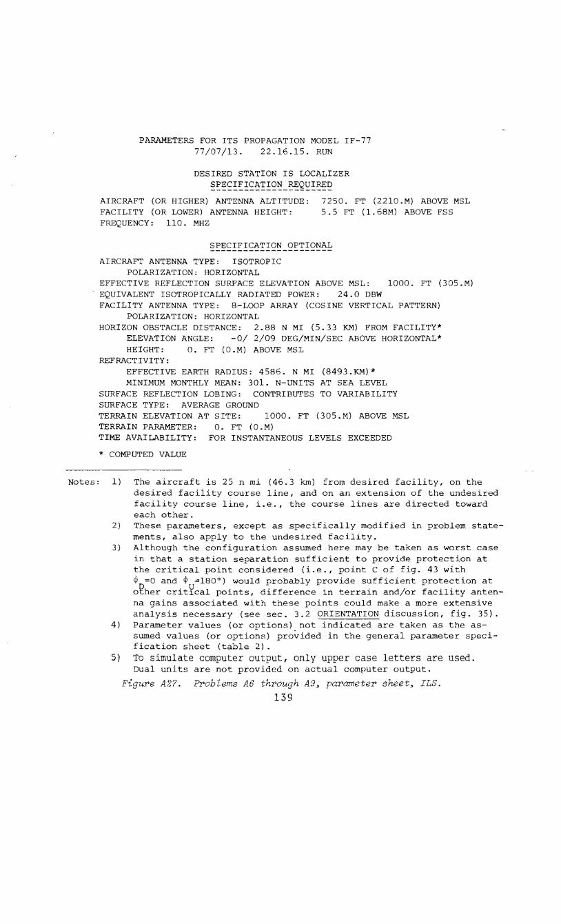
PARAMETERS FOR ITS PROPAGATION MODEL IF-77 77/07/13. 22.16.15. RUN
DESIRED STATION IS LOCALIZER
§~~~!~!~~!!~~-~g~!~~ AIRCRAFT (OR HIGHER) ANTENNA ALTITUDE: FACILITY (OR LOWER) ANTENNA HEIGHT: FREQUENCY: 110. MHZ
7250. FT (2210.M) ABOVE MSL 5.5 FT (1.68M) ABOVE FSS
SPECIFICATION OPTIONAL
AIRCRAFT ANTENNA TYPE: ISOTROPIC POLARIZATION: HORIZONTAL
EFFECTIVE REFLECTION SURFACE ELEVATION ABOVE MSL: 1000. FT (305.M) EQUIVALENT ISOTROPICALLY RADIATED POWER: 24.0 DBW FACILITY ANTENNA TYPE: 8-LOOP ARRAY (COSINE VERTICAL PATTERN)
POLARIZATION: HORIZONTAL HORIZON OBSTACLE DISTANCE: 2.88 N MI (5.33 KM) FROM FACILITY*
ELEVATION ANGLE: -0/ 2/09 DEG/MIN/SEC ABOVE HORIZONTAL* HEIGHT: 0. FT (O.M) ABOVE MSL
REFRACTIVITY: EFFECTIVE EARTH RADIUS: 4586. N MI (8493.KM)* MINIMUM MONTHLY MEAN: 301. N-UNITS AT SEA LEVEL
SURFACE REFLECTION LOBING: CONTRIBUTES TO VARIABILITY SURFACE TYPE: AVERAGE GROUND TERRAIN ELEVATION AT SITE: 1000. FT (305.M) ABOVE MSL TERRAIN PARAMETER: 0. FT (O.M) TIME AVAILABILITY: FOR INSTANTANEOUS LEVELS EXCEEDED
* COMPUTED VALUE
Notes: 1) The aircraft is 25 n mi (46.3 km) from desired facility, on the desired facility course line, and on an extension of the undesired facility course line, i.e., the course lines are directed toward each other.
2) These parameters, except as specifically modified in problem statements, also apply to the undesired facility.
3) Although the configuration assumed here may be taken as worst case in that a station separation sufficient to provide protection at the critical point considered (i.e., point C of fig. 43 with ~ =0 and ~ =180°) would probably provide sufficient protection at o~her crit~cal points, difference in terrain and/or facility antenna gains associated with these points could make a more extensive analysis necessary (see sec. 3.2 ORIENTATION discussion, fig. 35).
4) Parameter values (or options) not indicated are taken as the assumed values (or options) provided in the general parameter specification sheet (table 2).
5) To simulate computer output, only upper case letters are used. Dual units are not provided on actual computer output.
Figure A27. Problems A6 through A9~ parameter sheet~ ILS. 139
Solution: Examination of figure A26 shows that the aircraft
is at a constant elevation with respect to both mean-sea level
(msl) and the desired ILS site sur ce for all three parts of the
problem, but that aircraft elevation with respect to the undesired
ILS site surface changes for each part of the problem. Lower air
craft altitude with resnect to the undesired facility means that
the undesired signal level at the aircraft is expected to he
lower for a particular undesired facility-to-~ircraft distance
which will translate in the context of this 11rohlem to a decrease
in the station separation requirement. Conversely, a higher air
cr t altitude with respect to the undesired facility would be
expected to result in a larger station separation requirement.
Site surface elevations for various parts of the problem are
drawn as dashed lines in figure A26 and are extended from facility
to- ility to show that use of different site elevations is not
compatable with the use of a smooth earth for all of the terrain
between the facilities since different elevations result in dif-
rent earth radii. Desired and undesired signal levels are
computed independently for the parameters applicable to each
ility so that this difficulty is not recognized by the pro
grams, but must be considered in using the computer output. One
way to do this is to assume that each site elevation is valid at
least to the smooth earth horizon distance for its facility an
tenna and that the computed results are invalid when terrain at
the higher site elevation is visible to the other antenna. These
conditions are illustrated in figure A28 and result in a minimum
station separation (S . ) for which predictions are valid. Values - m1n for S . can be estimated from m1n
where s . == .V 2aHD +V2aH, +~ 2aHu mln ue
a= effective earth radius,
HD U =height of desired or undesired ' facility antenna above its site
surface elevation
140
(Al)

and ll 1n site el va tiOTlS*
Each term of (Al) is a smooth earth horizon type distance as il
lustrated in figure A28.
Figures A29 through ,:'\31 were deve1oped. fo1 thb problem and
the ration sPparation requirements resulting 1rom them 3re t
l:itcd l~elow alon~: with
Site Elevation Above msl
(ft CmL Desired Undesired
nnn
F
1,000(305)
1,000(305)
1,000(305)
2,000(610) A29
1,000(305) A30
0 A31
a
va1lJe:;:.:
e
141
btained fr m U):
uired Sttition ratio:1.
[nmi (km)J
100 (185)
l 7 (l 8
113 (209)
I l
[nmi (km)]
45 (83)
Not Apfllicablc
45 ( 8
\. /2nHU
S . = ~D ., 12aH + ~~ m 1 n t\e u
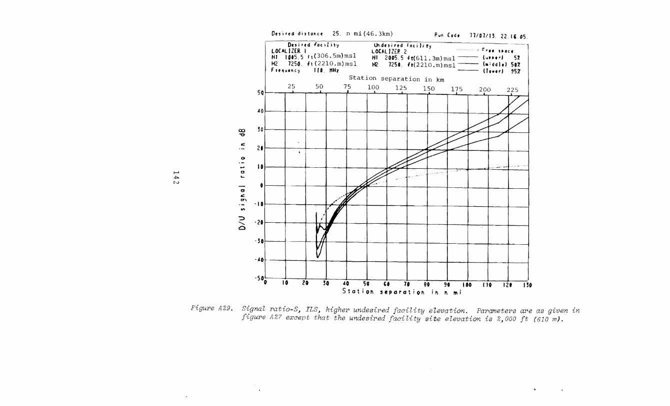
j-J
.j::>.
N
De,ired dis!o~~e 25. n mi(46.3km} Ru~ (odt 11101113. 22. 16.05.
--- ol;-i7ed (oc il i '~ Uri de ' i r r d I o ~ il i r~ ~-----
LOCALIZER I LOCALJZ£P. 2 .. '"•tt UOCt HI 1005.5 r 1 (306.5m)ms1 HI 20115.5 H(6ll. 3m)ms1 ___ ( ... -.. d 57. H2 7250. fl (2210.m)ms1 H2 1251. lt(2210.m)ms1 (•iddlt) 507. f rt1ut~C~ lfD. HH1 Oo•trJ 957.
Station separation in km 25 50 75 100 125 150 175 200 2i25 I • 50
I 40 / ~ CX) "0
,:; -
/~ t::/ v I
~ ...... v
~ v--I ---
30
21 0 --
•
~ r:---~ . .............. I .... 10 0 ....
-0 ,:; (T\ -...
"=> ......... C)
• 3
~ v . -~'' .•...•...... ...
h
"AI ,
,, I
/'Z I
~ ,
I
~ I
0
·I 0
·20
·4
I -s-o 10 zo !O 40 59 U 70 80 90 100 110 121 1!0 Station separation in n mi
Figure A29. Signal ratio-S~ ILS~ higher undesired ;acility elevation. Parameters are as given figure A2? except that the undesired facility site elevation is 2~000 ft (610 m).

Ouired di,ta11ce 25. n mi(46.3km) Ru11. Code 77101/13. 22. I G. 08. Ouired locility V11desired locilit~
............. I=' rtt S'OCt LCCALIZER I LOCALIZER 2 HI 1005.5 f: (306.5m}ms1 HI 1005.5 lt(306. 5m)ms1 luHtd 57. H2 7250. 1: (2210.m)msl li2 1250. f t(2210 .m)ms1 l~aiddltJ 507. l='recp .. ucy 110. ttHz llo-trl 957.
Station separation in km 25 50 75 100 125 150 175 200 225
I 1 5D
AD I /
CXl ~
-= -
/ ~ v I """
~ ~ l--- l.--7
I .....r: ~
30
20
0
·-1-' ... -!::> 0 tN L-
-0
-= ~
-"'
':) ........ 0
-1
~ ~ ~
~ ~
I • ......... ,A• .............
# ~ .... ······•···
....... · ...
I
,.,.· ~ I .' 1,
/"/ J
If' , I h
t'l
1 0
0
·2
·3
·l I
l -5.0 \D 20 30 lO 50 GO 70 80 90 100 110 1(0 130
Statior. separatior. ir. n ft'li
A.30. Signal ILS> equal site elevatz:ons. Parameters are as given in A27.
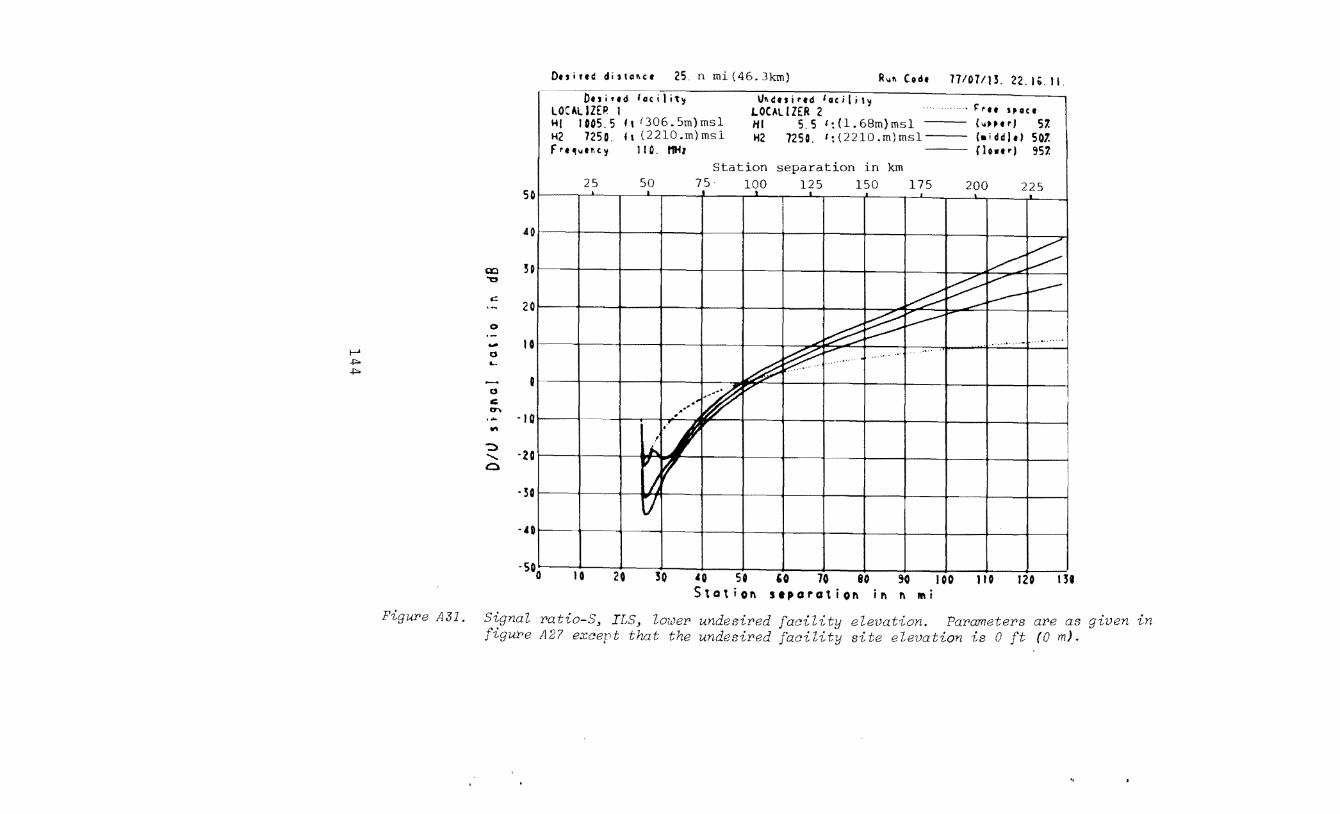
1-' +:» +:»
QQ "0
-=
0 --0 ....
-0 c 0"\
... ':) ........ 0.
'
50
40
30
20
10
0
·I 0
·20
·30
Ou i ud dis tallc t 25. n mi {46. 3km) R~11 Codt 17101115. 22. ''·II.
Ouirtd lacilit'l LOCALIZER 1 HI 1005.5 ft 1306.5m)ms1 H2 725G. lt (2210.m)msl f"rt~ufHij ]IQ. 11Hl
Vt~dtsirtd lacilil~ LOCAL llER 2 HI 5.5 it(l.68m}ms1
· .... l='ru s~act
(~Hf rJ 51. (aiddltl 507. Ch•••l ~57.
li2 7250. 1:{2210.m)ms1---
Station separation in km 50 25 225 75. 100 125 150 175
• ...1. 200
~ ~ ~ ,_. ...................... .
~ .............. ·····
-
v;r r7 ... c
-so 0 I 0 20 30 40 50 u 70 80 ~0 100 110 120 131
Statiol'l stparatiol'l in 1'1 1rd
FigUPe AJl. Signal ratio-S~ ILSJ lower undesired facility elevation. Parameters are as given in figu:r•e A27 exaept that the undesired lity site elevation is 0 ft (0 m).

ILS, Separations, Surface Constants
Problem A7: For the geometry illustrated by the equal site ele
vation portion of figure A26 and the ILS localizer parameters of
figure A27, determine the station separation required to ohtain
a 23 dB desired-to undesired localizer signal ratio at the air
craft with a time availability of 95 percent when the surf~ce con
stants (table S) are taken as those associated with (a) poor
ground, (b) average ground, (c) good ground, (d) fresh water, or
(e) sea water
Solution: Figures A32 through A36 were developed for this
problem, and the station separation requirements listed below
were taken from them.
Surface Type
Poor ground
Average ground
Good ground
Sea water
Fresh water
Hence, for this problem,
Figure
A32
A33
A34
A35
A36
surface type is
Station Separation [n mi (km2]
107 ( 19 8)
107 (198)
107 (198)
107 (198)
107 (198) .
not an important para-
meter. Other situations where vertical or circular polarization
and large (> 1°) grazing angles ($of fig. 40) are involved would
be expected to show greater dependence on surface type [49, figs.
III.l through III.8]. Even then the dependence may be masked by
surface roughness (probs. AS and AS), which makes the specular
reflection coefficients smaller as roughness increases.
145

Ouiu4 distcl\ct ZS. n mi(46.3km) Ru11 (odt 77/0l/13. 22. I G. 14.
l)u ired foe d i1y POOR 'ROIJNO
'Jl-.c~esiud locili\y ..... ;:-,,. , .. ,.
~· U05.5 lt(306.5m)ms1 Sou os dnirtd focility luHtrl 57. H2 7Z51. t t (2210 .m) ms1 laiddlt~ 507. ;:-,,~ .... 1\c;y 110. t1Hz n ... ,, 351.
Station in km
5 25 50 75 100 125 150 175 200 2t5 ~ I I
.co I /
en / ~ v L 3G
v
cr;:: - ~ r;: v-v '
......--::: 20 0 ·-
1-' -"""
0
Q'\ .._
-~ ~
~
h ······ ....... .............
I
~ .•
# .
..... . ····•··
I
I 0
0 cr;:: Ch -...
::> ........ C)
/~ 71 I ,"'
• I f.. ,. ,
A t r;
. \
·2
-3
-.c I
It -5~6 lO 20 30 '6 50 GO 70 80 '0 100 120 130 Ito
Station stporotion i~ n Mi
A3'2. r>atio-S,.ILS, gr>ound. Par>ameter>s ar>e in f1:aur>e A27

f-J .f::>. '-1
co -,;,
,;::
0
·-.... 0 ,_
0 ,;:: D"''
-.,.. ':)
' Q
Desired disto11ce 25. n mi{46.3km) R~o~11 Code 11101113. 22. l&. IG.
Ouirtd focili\~ -.vERAGE {.ROIM> HI IDDS.S lt(306.5m)ms1
V11 d u i red fa c i l i t ~
Saae as desired facility H2 72SO. ft (2210.m)ms1 ---
~ru HGtt
l~o~PHr) 51 <•iddltl 507. (Jo .. r) 957. ~ re quuq llO. HHz
Station separation in km 100 125 150 . 25
so 50 75 175 200 225
401------- /
H ~-20
10
0
~ ........... .~ ............ .. ~ .... L .. '··"·
-10
-20
-501-------
l7 -•o
-so 10 20 0 50 • • so u 70 80 90 '00 150 II 0 120
Statior. separatior. ir. r. ll'li
FiguY'e A.3.3. Signal raHo-8, average ground. Parameters aY'e as given in figur•e A2?.

50 I
40 I
Q) 30 I "'0
0::: - I 20 0
·-1-' ..... I 0 I .p. a co ...
- I 0 a 0::: cr. - -I 0 I ...
:::» ........ -20 I C)
-5 I
-l I
, -5.0
Duirtd ditlo!Ht 25. n mi(46.3km) R~~ Code 11101113. 22. K 18.
Ouirtd fc~eili\~ U11 du i r t d fa c i I i \ ~ ···· · ········ F'rtt tpact C.OOO 'ROVNO
HI 1005.5 ft(306.5m)ms1 Sou os dnirtd hcili\~ l~;p,ul 51. H2 1251. ft (22l0.m)ms1 lai ddltl 50'7. I=' rt ~~;ti\C~ 110. 11H: tlutrl 957.
Station separation in km 25 50 75 100 125 150 175 200 225 I.
/
/ ~ v ..,
~ ~ ~ v
........:: k---
~ V"":: ......-
~ v--
.......... , .... .............
~ ~ .... ·•······ ....... ....... ···'
......... ··
• I -K ~ ,
I
t'l I
-. 10 20 50 lO 50 '0 70 80 90 100 II 0 120 130 Stotiof'l seporotiof\ ir. r. 111i
Figure A34. Signal ratio-S, ILS, good gr•ound. ParameLers are as given in figure A27 except for surface
~

Dn i • e d d •' 1 o ~ c e 2 5. n rn i ( 4 6. 3 krn) R .. ~ Code 11/01/13. 22. tb. 59.
Du i • e d f o c ;t i t ~ V11clui~ed focilil':l ............ ' F"ru UCICt SEA 1111. TER
HI 1005.5 It (306.5rn)rnsl Saae os desired locilil~ ,,.,trl 57. H2 7250. It ( 2 210. rn) rns 1 laiddltl 501. F ''""'nc':l II 0. t1Hz llowtrl 957.
Station separation in krn 25 50 75 100 125 150 175 200 225
) .J.. _l t ' SD
I 40 /
CXl ~ v / "" 30
"0
,;: - ~ ~ ~ 1.-/
......-:::: l---20
0
·-1-' a ~ ,_ <-:::>
-a ,;: 17'\ -M
:::> ........ 0
It ~ ~ .....--
b .......... .... ,, ...........
# ~ .... •···· .. .. ····· ..
I •' ··•·· ...
I
-~ ! ,,""',...
• '/ i..
~ ,
1--- r;
0
- l D
·2
·50
·l I
I ·5~0 10 20 30 .co so GO 10 eo 9o 1 oo II 0 120 130 Stotior. separatiol'\ ir. 1\ ~ni
Y1:guPe A35. D1:gnaL Y'otio-S, ILS, sea water'. PaY'ametePs aPe m: g1:vr-!n in f1:guPe A27 except for' suPface
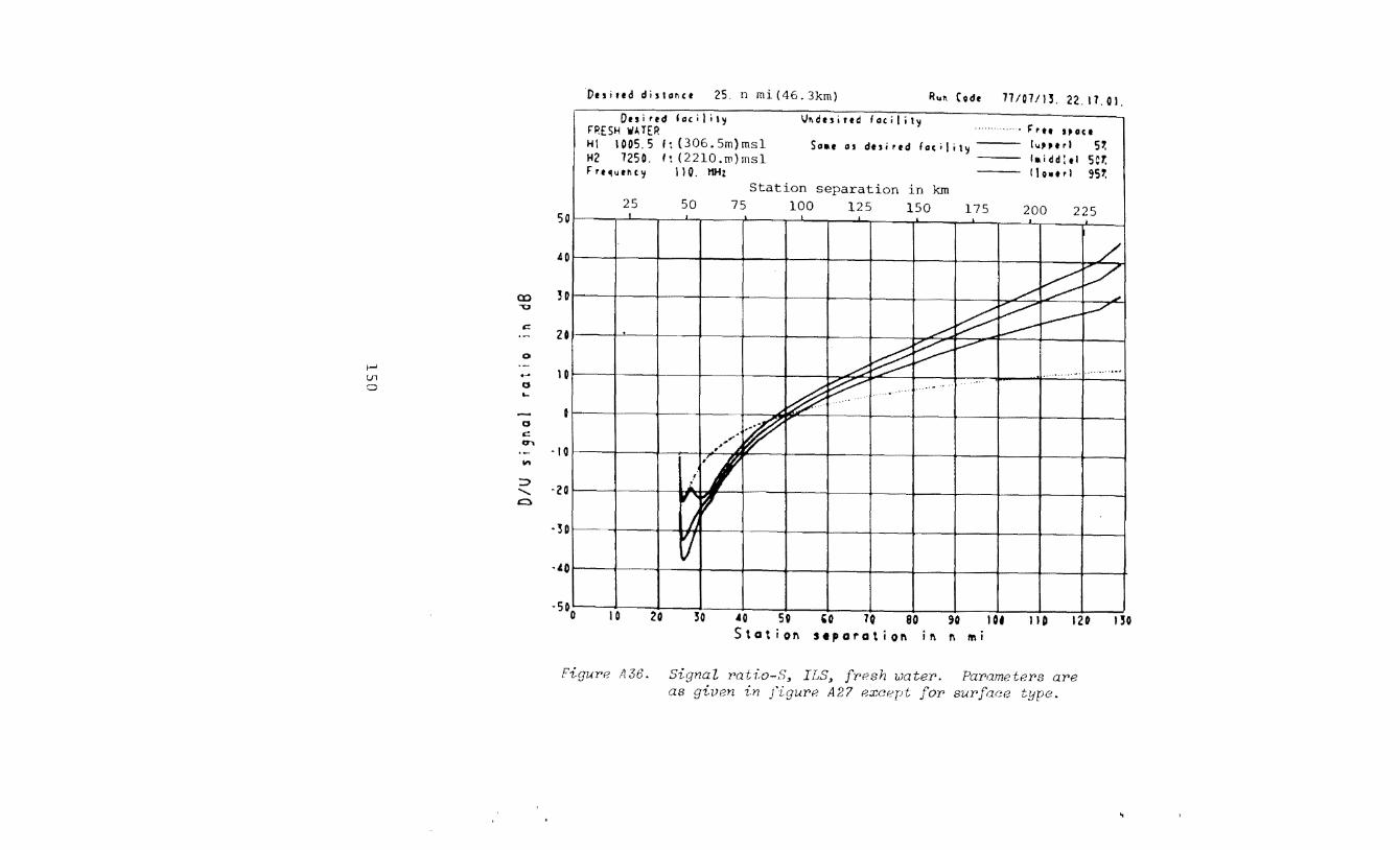
Dtsiltd dista~ct 25. n rni(46.3km) Ruft (odt 77/07/1,. 22. ll.Ol.
Ouirtd lacilit':l Vt~dtsirtd facility · ........ · · J:'ru nact ~P.ESH 'IIA.TER
HI 1005.5 ft{306.5m)msl Sou as dtsi rtd foe iIi 1':1 ["" t rl 51. H2 7250. It (2210.m)msl '•; ddl ., scr. Frt'lutnc':l II 0. 11Ht llutrl 951.
Station separation in km 25 50 75 100 125 150 175 200 225 I so
40 I /
(X) / ~ v 1 ""' H
"'0
c: - ~ ~ v-v I ...........:: 21
0
·-1-' .... tn 0 0 ....
-0 c: 0"\
-""
:::> ........ 0
~ ~ ,...--
) ~ ····· ...... ..............
~ ...... ··''
~ .. . ' •.... ' .
.. .... I
~ I ,)1.,.,.,.. ..
-,r/
I
a i.
" ,
l 0
- I Q
-20
·3 1-- ~ r;
·.t I
I -· ·5.0 I 0 20 '0 AO SD 'o 10 eo 90 101 llO 120 no Station separation inn nd
Figure 1136. Signal Pat?:o-8, ILS, fpesh water. Parameters are as given in ;'iguN< A27 except for surface .
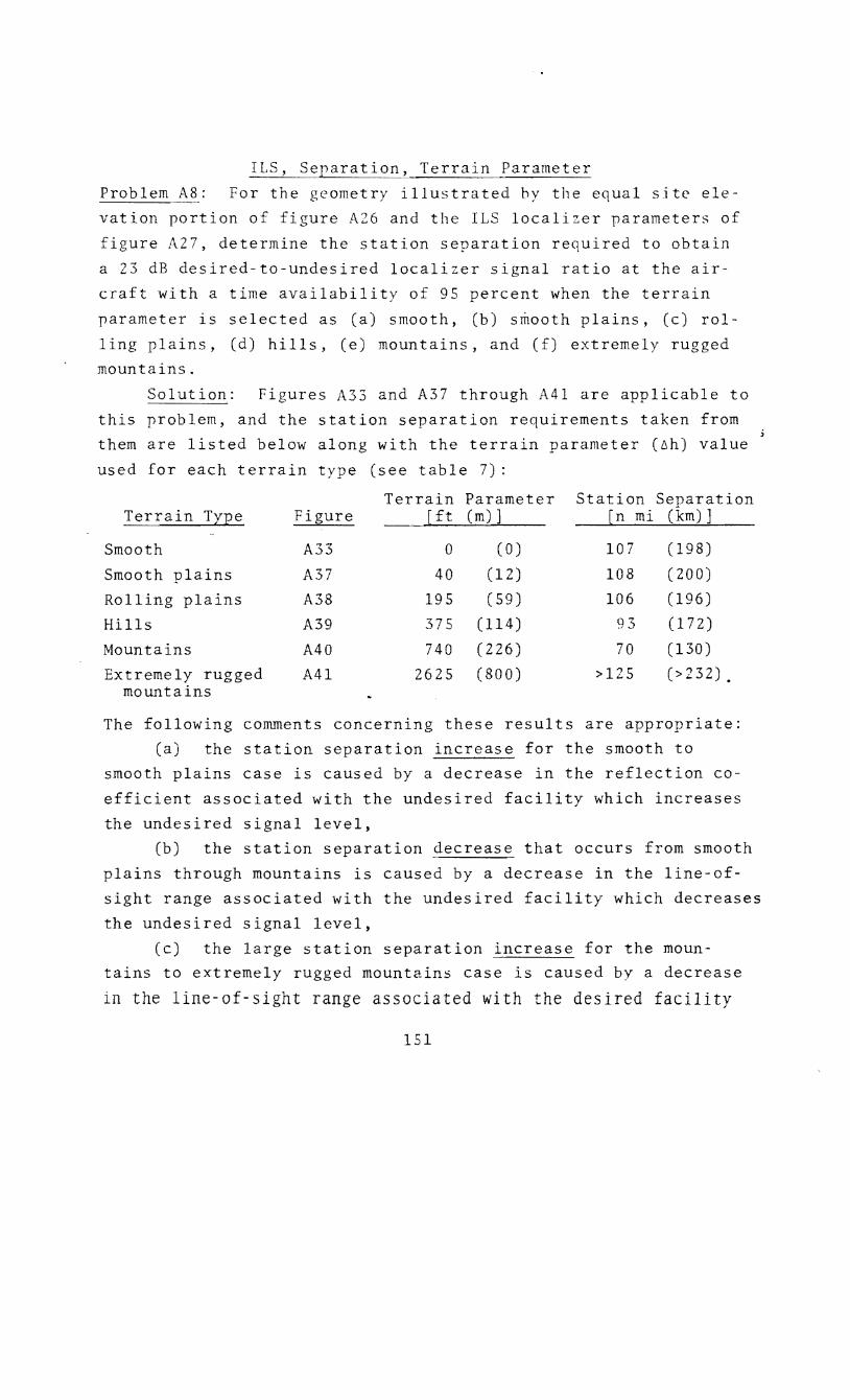
ILS, Separation, Terrain Parameter
Problem A8: For the geometry illustrated by the equal site ele
vation portion of gure A26 and the ILS localizer parameters of
figure A27, determine the station separation required to obtain
a 23 dB sired to-undesired localizer signal ratio at the air
craft with a time availability of 95 percent when the terrain
parameter is selected as (a) smooth, (b) smooth plains, (c) rol
ling plains, (d) hills, (e) mountains, and (f) extremely rugged
mountains.
Solution: Figures A33 and A37 through A41 are applicable to
this problem, and the station separation requirements taken from
them are listed below along with the terrain parameter (~h) value
used for each terrain type (see table 7):
Terrain Parameter Station Separation Terrain T_n~e Figure [ft (m)] [n mi (km)]
Smooth A33 0 (0) 107 (198)
Smooth plains A37 40 (12) 108 (200)
Rolling plains A38 195 (59) 106 (196)
Hills A39 375 (114) 93 (172)
Mountains A40 740 (226) 70 (130)
Extremely rugged A41 2625 (800) >125 (>232). mountains
The following comments concerning these results are appropriate:
(a) the station separation increase for the smooth to
smooth plains case is caused by a decrease in the reflection co
efficient associated with the undesired facility which increases
the undesired signal level,
(b) the station separation decrease that occurs from smooth
plains through mountains is caused by a decrease in the line-of
sight range associated with the undesired facility which decreases
the undesired signal level,
(c) the large station separation increase for the moun
tains to extremely rugged mountains case is caused by a decrease
in the line-of-sight range associated with the desired facility
151
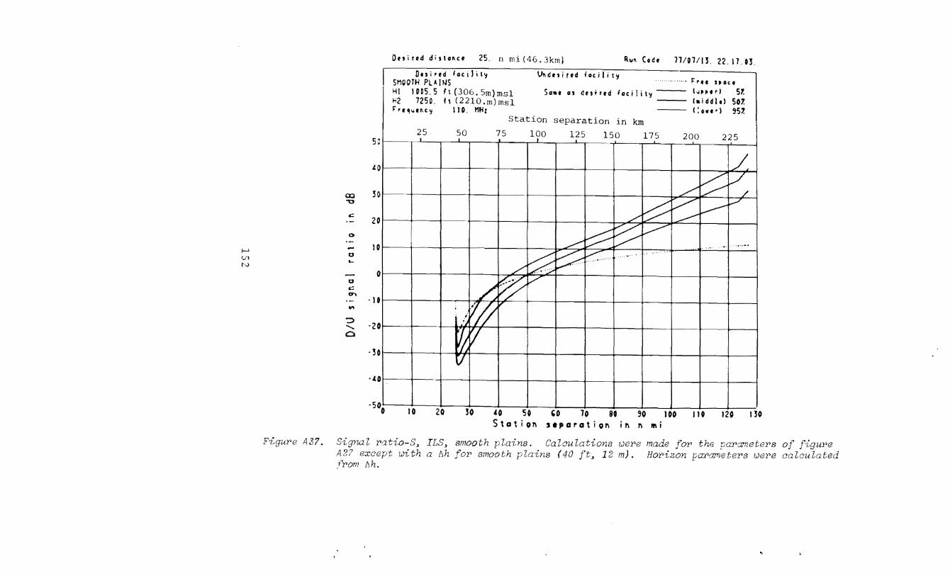
Ouiud distuce 25. n mi(46.3km) R"~ Code 11/07/ll. 22. 17. 03.
Duirtd facility v~ctsirtd iocili ly .... r:rtt HGct SMOQTJ.I PU..JJ.JS
HI 1~05.5 ft(306.5m)ms1 Saat as des•red facility luJPtrl 57. H2 7250. ft (2210.m)ms1 laiddltl 507. f •tqljt!\(~ 110. Ml-lz C:owt•) 957.
Station separation in km I
25 50 75 100 125 150 175 200 225 50
I .40 / cx::l
t;::: l/ / / 30 "0
.c::: - ~ v l.---v L ~ 20
0
·-f-.' -tn 0
N ....
-0 .c::: en -""
:::> ........ 0
-3
~ ~ ~
I ~ ~ ... ..... .........
~ ~ < .. ...... '
/ :::.G ~ j .
~ ~ ,/"
. _i ~ I
~ v I
[/
10
0
·10
·20
·I. I
40 50 '0 70 80 90 JOO I ·STO
10 20 30 no 120 130 Station separation inn mi
F1:gure A37. 8ignal ratio-8" IL8" smooth plains. Calculations were made for the parconeters of f1:gure A27 except th a Ah for smooth plains (40ft" 12m). Horizon pa:t'ameters were calculated _rY.om !',h.
~

f-1 U1 VI
co ""0
-= 0
·--0 L-
0
-= en
"' '::> ........... a
so
40
50
20
I 0
0
-I 0
-20
-50
Desired dis!a~ce 25. n mi(46.3km) ~~~ Code 77/07/15. 22. 17.05.
Oesirtd facilit!:! v~desirec facilit!:i ROLLINCi PL.t.INS ···· ·········· f."rtt HOC I
HI 1005.5 ft(306.5m)ms1 Sou as desired facilit~ I~Htrl 5% H2 7250. It (2210.m)ms1 laiddlt) 507. f."req ... t~c!:l 110. 11Hz , . . . llo111trl 957.
Station separation ~n km
25 so 75 100 125 1so 175 200 225
)jV ~/j
/~/v v-vv
......... ~ -- / ................. . VI,_....,.... I/ .... . / ~~·:J;;?~ ....... .
hV:V~ ~~~ ~v v
-40 ~---+----~----~---+----~----~--~----~--~~---L----~---- -----
-500 10 20 50 AO 50 c;o 70 80 90 lOt 110 120 150 Station separation in n rni
FiguPe AJB. Signal Patio-S~ ILS~ Polling plains. Calculations wePe made foP the paPametePs of figuPe A27 except with a 6h foP Polling plains (195 ft~ 59 m). HoPizon paPametePs uJel1 e calculated fPom 6h.
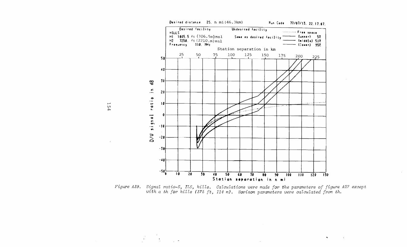
Ouired disto~ct 25. n rni(46.3km} Run Code 71/01/13. 22.17.07.
Ollired r iIi ty Vndtsited focillty ............. F'rtt ''ott HILLS
HI 1005. 5 It ( 306. 5rn) rns1 So•e os desired locility (""' r) 57. H2 nso. rt (2210.rn}rns1 (•iddlt) 501. F're~ ... e~cy 110. tlHt CluerJ 951.
Station separation in km
25 50 75 100 125 150 175 200 225
' I _1_ so
I .40 V£ / lXI "'0
,::: -
I ~ v I .L '/ ~
'50
20 0
·-....... -tn 0 .p. ._
-0 ,::: 0'\ -"'
::;, ........ 0
·3
I ~ / ~ . ····· ....... ············· / ~ ;;/ , .. ·•"' .. ...........
/ ~ I ...-
h v ~ I /
' !J ~ ~ I
IIJ
0
-IG
·20
-I. )
I ·5 •• 10 20 30 .CO 50 U lO 80 90 I 00 II 0 120 130 Statio!\ stparatiol\ il\ n mi
Figure A39. Signal ratio-S, hills. Ca lations were for the parameters of figure A27 except with a 6h for lls (375 114m). Horizon parameters were calculated from 6h.
"
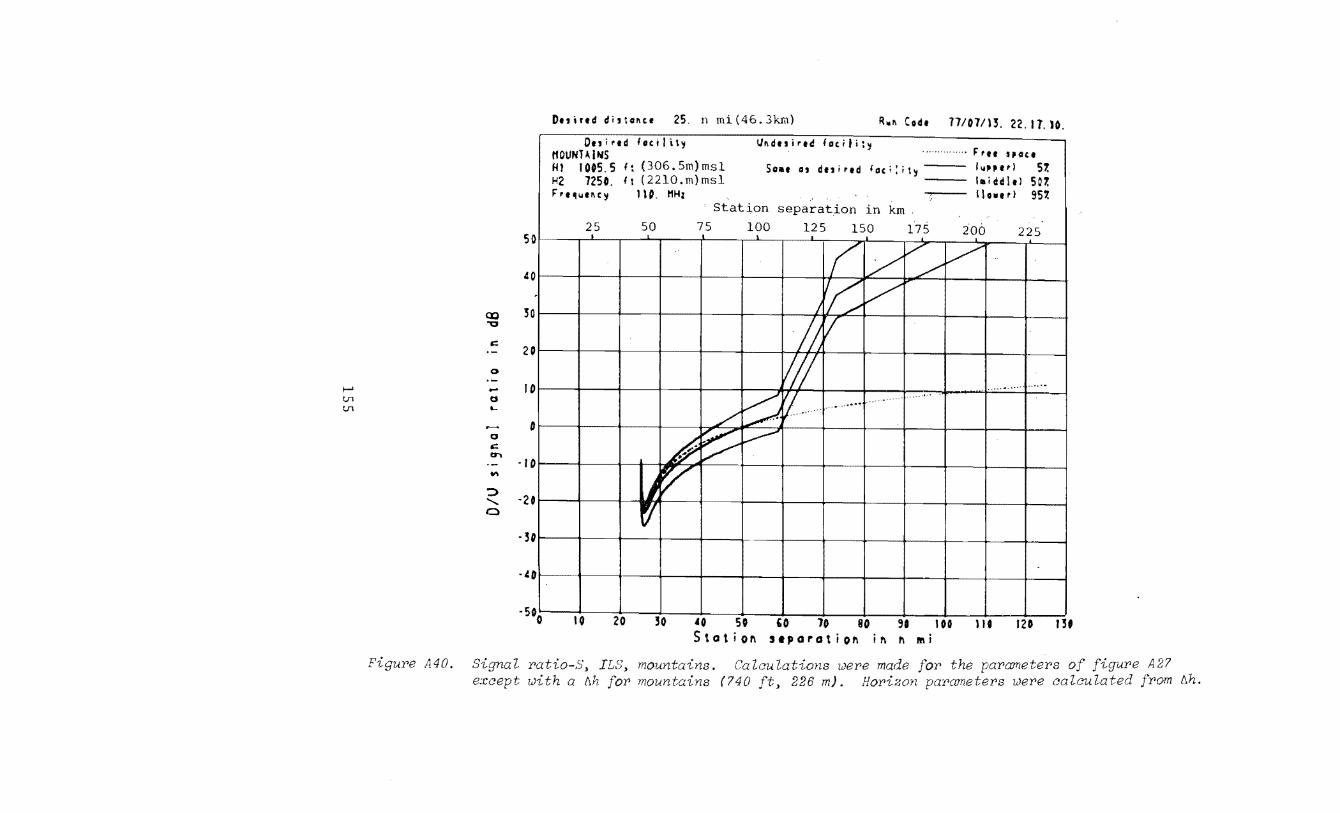
50 I
40
Q'J 30 "0
r;:: - I 20
0
·-~ .... ' 10 Vl a Vl t-
- 0 I a r;:: 17"\
- • 10 I If\
::>
' I -20 0
·30 I
·40 ~
~ -5~0
;140. except
Du,rtd di'U"'" 25. n mi(46.3km) R.,.. Codt 77107/)3. 22. 17. 10.
Oui~td locili.~y ll11duired facility ............... f:" 'tt 'POet rt OliNH I tiS
f.jJ 1005.5 ft (306.5m)ms1 So•t "' dt'i'td laci:ity ~. .. ,,.,, 57. H2 7250. ft (2210.m}ms1 l•iddltl 507. F,t~utl\cy IU. I1H1 II nt, I 951.
Station separation in km .
25 50 75 100 125 150 175 200 225
L v v v /
j ~ v I! :;
1/1 . ............. ........
v, fj ··"' ····•·· .......... ./ ~
... -·····
~ ~ v ~ J v ~ I
!
I
10 20 30 .CO 50 £0 10 80 ,. IOD )It 120 131
for>
Station separation inn nd
Ca (?40
A2?
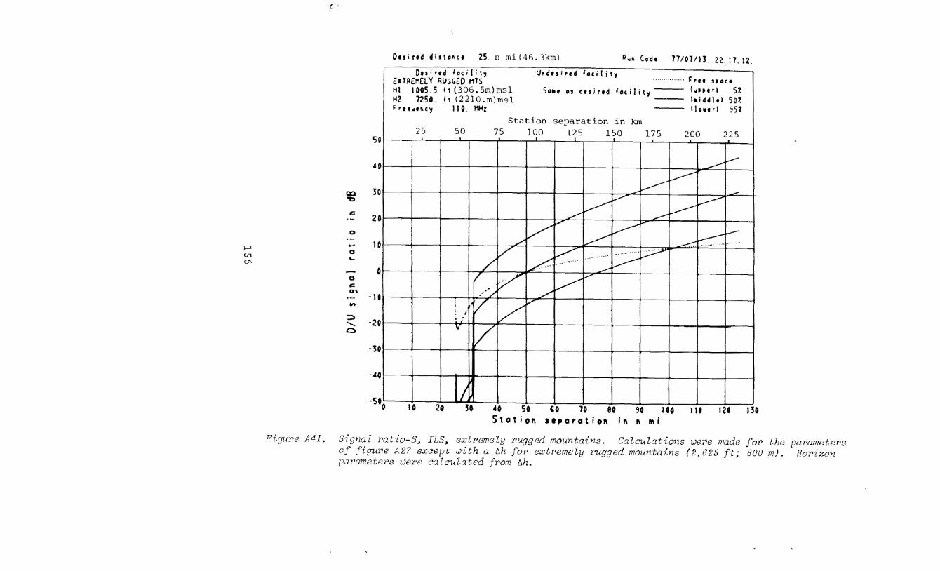
(
.... tn 0.
Figure A 41.
Onirtd distollct 25. n mi{46.3km) R~11 Codt 17101113. 22. 17. 12.
Du i rtd foe iIi t~ EXTREMEL~ RUGGED MlS
u~dtsirtd foci[ity ............. f:'rtt HOCI
HI 1005.5 ft(306.5m)msl Sou os dtsirtd focilit~ f~o~Htrl 5% H2 1250. ft (22lO.m)msl l•idclltl 507. F' rt~~o~UC~ II 0. 11Hz llntrl 957
Station separation in km 25 50 75 100 1~5 150 175 200 225 so
AD ---v
en "D
1:! -0
·--a ....
-a 1:! cr. -....
::;:)
' c
. \
v-~ I I --v v ~ I ~ ~ ~
/ v v ~ .----- ....-
I I / ~ ... ,, ........ / ~··· , .............
.~" .... ' ..... ~ ! / / v--I . ,........
/ / /"' v
.---/ ./ I
/ / v
i .. I ,.-
/ I
I
30
20
lD
0
·20
·3
·A I
D j_
--·5.0 10 20 30 •o so u 10 eo 90 uo Ill 121 130 Stotiofl stporotior~ ifl "11d
Sigr~l ratio-S~ ILSJ extremely rugged mountains. Calculations were made for of figure A2? except with a 6h for extremely rugged mountains (2J625 ft; BOO pa1'ameter<s wer•e calculated from D.h.
the parameters Horizon

which decreases the desired signal level, and
(d) the exclusive use of nh to describe terrain could easily
result in station separations that are not appropriate for speci
fic paths. Actual horizon information should be used whenever it
is available.
ILS, Separation, Terrain Profile
Problem A9: For geometry similar to the equal site elevation por
tion of figure A26 and the equipment parameters of figure A27,
determine the station separation required to obtain a 23 dB de
sired-to-undesired localizer signal ratio at the aircraft with a
time availability of 95 percent when terrain parameters are de
termined using (a) topographic mars and (b) the Electromagnetic
Compa~ibility Analysis Center (ECAC) terrain file. Sites should
be selected to have equal elevations as shown by topographic maps,
and the terrain between them should be "severe".
Solution: Locations at Seattle (47°15'00"N, 122°22'47"W)
and Portland (45°33'22"N, 122°30'25"\11) were selected for the de
sired and undesired ilities, respectively. These locations
were selected based on the problem requirements for equal site
elevations and severe terrain from paths for which topographic
profile data are available on £omputer cards [39, fig. 2.22]. It
is unlikely that these particular locations would ever actually
be selected as localizer sites.
In calculating the desired signal level at the aircraft, only
terrain characteristics associated with the desired facility are
used, and beyond the facility horizon obstacle the terrain is ta
ken as smooth with an elevation equal to the effective reflecting
surface elevation for the desired facility. Similar considera
tions are involved in the calculations of the undesired signal
level. Hence, actual terrain between the facility horizon ob
stacles is not involved in station separation calculations since
only terrain between each facility and its horizon obstacle is
utilized to determine key terrain characteristics.
157
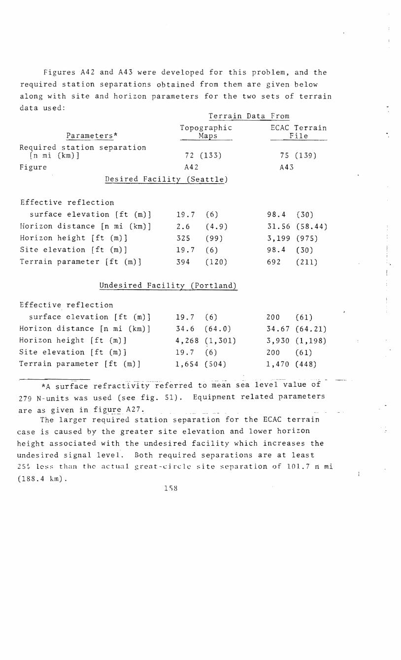
Figures A42 and A43 were developed for this problem, and the
required station separations obtained from them are given below
along with site and horizon parameters for the two sets of terrain
data used: Terrain Data From
Parameters*
Required station separation [n mi (km)]
Figure
Topographic Maps
72 (133)
A42
Desired Facility (Seattle)
Effective reflection
surface elevation [ft (m)] 19.7 (6) Horizon distance [n mi (km)] 2.6 (4.9) Horizon height [ft (m)J 325 (99) Site elevation [ft (m)] 19.7 (6) Terrain parameter [ft (m)] 394 (120)
Undesired Facility (Portland)
Effective reflection
surface elevation [ft (m)] 19.7 (6) Horizon distance [n mi (km)] 34.6 (64.0) Horizon height [ft (m)] 4,268 (1,301) Site elevation [ft (m)] 19.7 (6) Terrain parameter [ft (m)] 1,654 (504)
*A surface refract1viti- r-eferred to niean sea
ECAC Terrain File
75 (139)
A43
98.4 (30)
31.56 (58.44)
3,199 (9 7 5) 98.4 (30)
692 (211)
200 (61) 34.67 (64.21)
3,930 (1,198)
200 (61) 1,470 (448)
-
level value of
279 N units was used (see fig. 51). Equipment related parameters
are as given in figur~ A27~ The larger required station separation for the ECAC terrain
case is caused by the greater site elevation and lower horizon
height associated with the undesired facility which increases the
undesired signal level. Both required separations are at least 25~ lc~~ than the actual great c:irc1c site separation of 101.7 :ri mi
(188. 4 km) . 1S8
..

Q) "'Q
,;: -0
·-........ .... (Jl a t.D ...
-a ,;: cr. -"' ~ ........ 0
,..,. rtpure A42.
I so
40 I
I 30
20
10
0
-10
-20 I
·30 )
·lO )
~ ·Sw0
Desired disto11ce 25. n mi(46.3km) R ... 11 Code 71/01113. 22.11. 13.
Ouired locilit~ SEATTLE
Vlldttired locilit~ PORTLAND ............ F'ru HUe
HI 25. 2 It (7. 7m) ms1 ~I 25.2 ft(7. 7m)ms1 ,.,.,.,, 51. H2 G2711. f t ( 1911. m) ms1 H2 (aiddhl 501. G21D. it(191l.m)ms1 F're111otiiC~ I It. 11Hz II ower) 951.
25
I 0 20
Station separation in km· 50 75 100. 125 150 175 200 225
-~
~ --- ~ f.-..-" ..----~ ~
. ········ .... .......
v-- ... ······ ~ .......... ........
...-k<: ~ ~
........ ~
~ ~ ,.,.,.....
~ io""'
/; ·.
~ l
-----
3G .CO 50 GO 10 80 90 100 110 121 13D Statio~ separatio~ i~ ~ mi
Signal rat?:o-5, TDS, th fr>om topo(:rr'aph?;c maps (see t;c:;xt). Equipment parame ter>s ar>e as g<:ven in fig.UY'e A2?. The sharp incN'!I1Se "J/U YJ.ear> ?0 n
30 km) response to a sharp decr>ease in the undesir>ed sipnal level occur>s as of sight cond1: tions ar>e lost overo the li ty to path fips. 113? throur.rh .441).
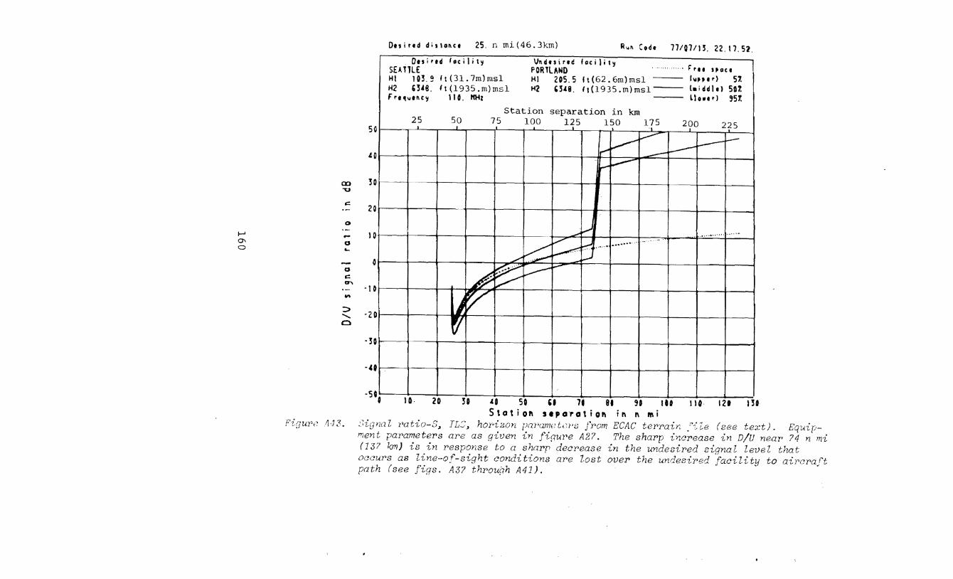
en "U
.::: -0
·-f-1 0\ 0 0 ....
-0 c a-.. -....
:::> ........ 0
Figur>e !J·J3.
Duired dis\ol\ct 25. n mi(46.3km) Rw~ Codt 77107/l~. 22. 17.52 .
. Oui•td focility Vl\dts i rtd foe il i ty · ..... ····· · J:'ru sPace SEA TllE PORTLAND
HI 103. 9 It ( 31. 7m) ms1 HI 205.5 ft(62.6m)ms1 IIIHtd 57. 1-12 '348. It (1935 .m)ms1 H2 G348. 1!(1935.m)ms1 l•iddh) 507. F •• 4!YII\C y II 0. l'tHt Ll .. t•l '51.
Station separation in km 25 50 75 100 125 150 175 200 225 I 50
v---~ ~ f.--,.,.... ~ I ,.......-.40 ,...... ~
I 30
20
'
.,
............ ............. .... ·-~ .............. ·····' ....
~ ~ ~ ......
/ .-'
~ ~ .....--- !-'"""
v lJ v
I r
I 0
0
·I 0
·3 I
-.c 1~-
I ·S.t 10 20 30 .co 50 U lt 81 'I IU 110 120 130
Stotiol\ stporotiol\ il\ 1\ l'fti l r'atio-S~ JL:.;~ hor·i;:;on pm•ame to•s j'r>om ECAC ter>rain ."'i (see text). Equ-ip
ment parameters ar>e as given in figuPe A27. The sharp increase in D/U near• 74 n mi (13? km) is in r>esponse to a sharp decrease in the undesired signal level that occur>s as line-of-sight conditions ar>e Z.ost over the undesired facility to aircraft path (see figs. AJ? throuph A41).
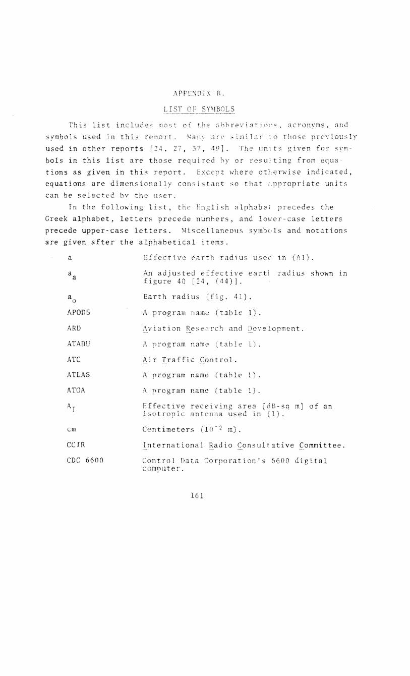
LT OF S s
This list in 1 r of th
symbol.s used in th s rencrt. \ian~o a~·c :' miLlr :o those JHC'\'iously
d · th t r-"' ,..,,., -_, use ::tn o _,("r repor s r-.-+. ~.- 1, .) .• 4 J • T un1ts given
bols in this list are those required hy or resu~ting from equa
tions as given in this report. Exc t where otl erwise indi ated,
equations are dimensionally consistant so that :.ppropriate units
can be selected ser.
In the following l st, the lish alp et prece s the
Greek alphabet, letters precede numbers, lo~er case letters
precede upper-case letters. '\!iscellaneous symbc,ls and notations
are given after the alphabetical items.
a
a a
APODS
ARD
ATADU
ATC
ATLAS
ATOA
ern
CCIR
CDC 6600
Ef ctive earth radius used in (A1).
An adjusted e figure 40 [24,
ctive eJ.rtl ( 44) ] .
Earth radius ( . 41).
A program name (t le 1).
radius shown in
Aviation ReseJrch and Development.
A program name table 1).
Air Traffic Control.
A program name (tahle 1).
A program name (t le 1).
Effective receiving area [dB-sq m] of an isotropic antenna used in (1).
Centimeters 10-~ m).
International Radio Consultative Committee.
Control nata orporation's 6600 digital uter.
161
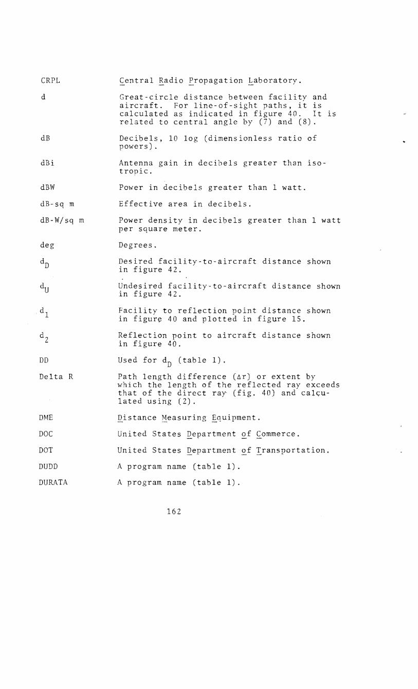
CRPL
d
dB
dBi
dBW
dB-sq m
dB-W/sq m
deg
dD
du
dl
d2
DD
Delta R
DME
DOC
DOT
DUDD
DURATA
Central ~adio Propagation Laboratory.
Great circle distance between facility and aircraft. For line-of-sight paths, it is calculated as indicated in figure 40. It is related to central angle by (7) and (8).
Decibels, 10 log (dimensionless ratio of powers).
Antenna gain in decibels greater than isotropic.
Power in decibels greater than 1 watt.
Effective area in decibels.
Power density in decibels greater than 1 watt per square meter.
Degrees.
Desired facility-to-aircraft distance shown in figure 42.
Undesired facility-to-aircraft distance shown in figure 42.
Facility to reflection point distance shown in figur~ 40 and plotted in figure 15.
Reflection point to aircraft distance shown in figure 40.
Used for dD (table 1).
Path length difference (6r) or extent by which the length of the reflected ray exceeds that of the direct ray (fig. 40) and calculated using (2).
Qistance ~easuring E_quipment.
United States Qepartment of Commerce.
United States Qepartment of Iransportation.
A program name (table 1) .
A program name (table 1) .
162
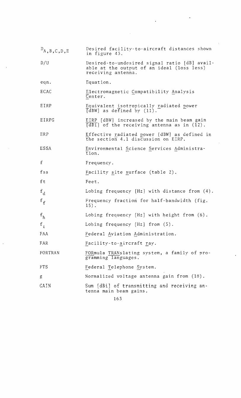
D A,B,C,D,E
D/U
eqn.
ECAC
EIRP
EIRPG
ERP
ESSA
f
fss
ft
FAR
FORTRi\N
FTS
g
GAIN
Desired facilitv to-aircraft distances shown in figure 43. '
Desired-to-undesired signal ratio [dB] avail able at the output of an ideal (loss less) receiving antenna.
Equation.
Electromagnetic ~ompatibility ~nalysis Center.
Equivalent isotropically radiated power TdBW] as defined by (11) .- -
EIRP (dBW] increased by the main beam gain TdBIJ of the receiving antenna as in (12).
Effective radiated power [dBW] as defined in the section 4.1 discussion on EIRP.
Environmental Science Services Administration.
Frequency.
Facility site surface (table 2).
Feet.
Lobing frequency [Hz] with distance from (4).
Frequency fraction for half-bandwidth (fig. 15) .
Lobing frequency [Hz] with height from (6).
Lobing frequency [Hz] from (5).
Federal Aviation Administration.
facility-to-~ircraft ray.
FORmula T~~Nslating system, a family of programming languages.
federal Telephone §ystem.
Normalized voltage antenna gain from (10).
Sum [dBi] of transmitting and receiving antenna main beam gains.
163
GCPP
GHz
GOES
GPO
hr
HI POD
Hz
Hl
HZ
in
IEEE
IF-73
IF-77
ILS
ITS
IRE
JTAC
~reat-£ircle £ath ~lane.
Gigahertz (109 Hz).
Geostationary Operational Environmental Satellite. -
Government ~rinting Office.
Gain [dBi} of the receiving antenna main b e am for (12 ) or (13) .
Gain [dBi] of the transmitting antenna main beam for (11) or (13).
IIour.
A program name (table 1).
Hertz.
Facility antenna height above fss or msl.
Aircraft altitude above msl.
Height of desired or undesired facility antenna above its site surface. Used in (Al).
Antenna elevations above the reflecting surface shown in figure 40.
Significant wave height.of table 6.
Magnitude of the difference in site eleva tions. Used in (Al).
Inches.
Institute of Electrical and Electronic Engineers.
ITS-FAA-1973 propagation model.
ITS-FAA-1977 propagation model.
Instrument Landing ~ystem.
Institute for Telecommunication Sciences.
Institute of ~adio Engineers.
Joint Technical Advisory Committee.
164
kHz
km
kts
log
LOBING
m
mhos
min
mm
msl
MHz
n
n mi
nsec
NBS
NDLF
NHLF
NOAA
NTIS
N 0
Kilohertz (103Hz).
Kilometer (103m).
Knots [n mi/hr].
Common (base 10) logarithm.
A computer program (table 1).
Basic transmission loss [dB] level not exceeded for 95% of the time.
Meters.
Unit of conductance or siemens.
Minutes.
Millimeters (lo-3 m).
Mean sea level.
Megahertz (105 Hz).
A power used in the ionospheric scintillation frequency scaling factor discussion of section 4.1.
Nautical miles.
Nanoseconds (lo- 9 sec).
National Bureau of Standards.
Normalized distance lobing frequency used in ( 4) .
Normalized height lobing frequency used in ( 6) •
National Qceanic and ~tmospheric ~dministration.
National Technical Information Service.
Minimum monthly mean surface refractivity (N-units) referred to mean sea level from figure 51 or 52.
165
N s
N-units
Prob.
PTR
rad
rms
r 0
RTA-2
sec
sq m
s mi
s
SHF
SRVLUM
s . m1n
t1inimum monthly surface refractivity [N-units] (sec. 4.1, refractivity discussion).
Units of refractivity [4, sec. 1.3] corresponding to (refractive index -1) x 10 6 .
Problem.
Power available [dBW] at the output of an ideal (loss less) isotropic receiving antenna from (1).
Total radiated power [dBW] used in (11).
Radians.
Root mean square.
Direct ray length shown in figure 40.
Segments of reflected ray path shown in figure 40 and components of r 12 .
. Reflected ray path length as shown in figure 40.
A TACAN facility antenna type.
Seconds.
Square meters.
Statute miles.
Station separation shown in gures 42 and 43, and calculated from (9).
~uper-High ~requency (3 to 30 GHz).
A program name (table 1) .
Facility separation shown in figures 42 and 4 3.
Minimum valid station separation calculated from (Al).
Power density at receiving antenna [dB-W/sq m] used in (1).
166
TACAN
THz
TWIRL
UHF
VHF
VOR
aA,B,D,D,E
t:.h
t:.r
0 e
8 t
8 0
TACtical Air Navigation, an air navigation aid used to provide aircraft with distance and bearing information.
Terahertz (1012Hz or 106 MHz).
A program name (table 1).
Ultra-~igh Frequency (300 to 3000 ~fifz).
~ery !i_igh Frequency (30 to 300 Milz).
VHF Omni Directional Range, an air navigation aid used to provide aircraft with bearing information.
Volts per volt.
Magnitude of aircraft radial velocity for ( 4) .
Magnitude of aircraft vertical ascent rate for (6).
Angles identified in figure 43.
Terrain parameter used to charcterize terrain, from table 7 or figure 53.
Path length difference for rays shown in fig ure 40 and calculated using (2).
Angle between direct ray and reflected ray at the facility as shown 1n figure 40.
Ray elevation angle used in (10).
Direct ray elevation angle shown in figure 4 0.
Half power beam-width of facility with JTAC antenna pattern, used in (10).
Beam tilt above horizontal of facility antenna, used in (10).
Central angle shown in figure 41 and used in (7) and (8).
Root-mean-square deviation of surface excursions within the limits of the first Fresnel zone in the dominant reflecting plane from table 6.
167

T
Wavelength.
Time lag [nsec] of reflected ray with re spect to the direct ray, om (3).
Angles defined in figure 43.
Grazing angle shown in figure 40.
Degrees, e.g. 12°.
Degrees celsius.
168

[ 1]
[ 2]
[3]
[ 4]
[5]
[6]
[ 7 J
[ 8 J
[9]
[10]
[11]
[12]
REFERE:-JCES
Ames, L.A., P. Newman, and T. F. Rogers (1955), VHF tropospheric overwater measurements for beyond the radio h or i z on , Pro c . IRE , ±i, No . 1 0 , 13 6 9 - 13 7 3 .
Barnett, W. T. (1972), 1v1ultipath propagation at 4, 6, and 11 GHz, Bell Sys. Tech. J. 51, No. 2, 321-361.
Bean, B. R., B. A. Cahoon, C. A. Samson, and G. D. Thayer (1966), A World Atlas of Atmospheric Radio Re fractivity, ESSA Mono. 1 (GP0) 1 •
Bean, B. R., and E. J. Dutton (1968), Radio Meteorology (Dover Publications, Inc., New York, N.Y.).
l
Bean, B. R., J. D. Horn, and A.M. Ozanich, Jr. (1960), Climatic Charts and Data of the Radio Refractive Index for the United States and the World, NBS Mono. 22 (GP0) 1 •
Bean, B. R., and G. D. Thayer (1959), CRPL Exponential Reference Atmosphere, NBS Mono. 4 (GPO) 1 •
Beard, C. I. (1961), Coherent and incoherent scattering of microwaves from the ocean, IRE Trans. Ant. Prop. AP-9, No. 5, 470-483.
Beckmann, P., and A. Spizzichino (1963), The Scattering of Electromagnetic Waves from Rough Surfaces, Internat1. Series of Monographs on Electromagnetic Waves ~(Pergamon Press, New York, N.Y.).
CCIR (1975), Propagation data required for trans-horizon radio-relay systems, Rept. 238-2, XIIIth Plenary Assembly, Geneva (Int1. Telecomm. Union, Geneva).
Crane, R. K. (1971), Propagation phenomena affecting satellite communication systems operating in the centimeter and millimeter wavelength bands, Proc. IEEE 22_, No. 2, 173-188.
Dougherty, H. T. (1967), Microwave fading with airborne terminals, ESSA Tech. Rept. IER 58-ITSA 55 (NTIS, N-70-73581) 2 •
FAA (1963), TACAN ground station equipment, FAA specification3, FAA-E 2006.
169
[ 13]
[14]
[15]
[16]
[17]
[18]
[19]
[20]
[21]
[ 2 2]
[ 2 3]
FAA (1_965), VHF/UHF Air/Ground Communications Frequency Engineering Handbook, FAA Handbook 3 , 6050.4A.
FAA (1965), Radio Frequency Hanagement Principles and Practices; General, Organization and Functions, FAA Handbook3, 6050.8.
FAA (1969), Frequency Management Engineering Princinles; Geographical Separation Criteria for VOR, DME, TACAN, ILS, anJ VOT Prcquency Assignments, FAA Ilnndhook 3 ,
6050.5A.
FAA (1969), Frequency Management Principles Spectrum Engineering Measurements, FAA Ilandbook 3 , 6050.23.
FAA (1975), DME ground station equipment terminal area, FAA specification 3 , FAA-E-2444-A.
Frisbie, F~ L., D. J. Hamilton, C. D. Innes, F. S. Kadi, and G. M. Karren (1969), A comparative analysis of selected technical characteristics for several frequency bands available to aeronautical satellite services, Unpublished 4 FAA Report 3 .
Gierhart, G. D., A. P. Barsis, M. E. Johnson, E. M. Gray, and F. M. Capps (1971), Analysis of air ground radio wave propagation measurements at 800 MHz, OT Telecomm. Res. and Engrg. Rept. OT/TRER 21 (NTIS, COM-75-10830/AS) . 2
Gierhart, G. D., and M. E. Johnson (1967), Inter renee predictions for VHF/UHF air navigation aids, ESSA Tech. Rept. IER 26 ITSA 26 (NTIS, AD 654 924) 2 •
Gierhart, G. D., and M. E. Johnson (1969), Transmission loss atlas for select aeronautical service bands from 0.125 to 15.5 GHz, ESSA Tech. Rept. ERL 111 ITS 79 (GPO) 1 •
Gierhart, G. D., and M. E. Johnson (1971), Interference predictions for VHF/UHF air navigation aids (supplement to IER 26 ITSA 26 and ERL 138-ITS 95), OT Telecomm. Tech. Memo. OT/ITSTM 19 (NTIS, AD 718 465) 2 .
Gierhart, G. D., and M. E. Johnson (1972), UHF transmis sion loss estimates for GOES, OT Telecomm. Tech. Memo. OT TM-109 (NTIS, COM-73-10339) 2 •
[24] Gierhart, G. D., and M. E. Johnson (1973), Computer nrc-grams for air/ground propagation and interference analysis, 0.1 to 20 GHz, DOT Rent. FAA-RD-73-103 (NTIS, AD 770 335)2. -
170
[25] Gierhart, G. D., and M. E. Johnson (1973), Pronagation model (0.1 to 20 Gllz) extensions for 1977 computer programs, DOT Rept. FAA RD 77-129.
[26] Gierhart, G. D., R. W. Hubbard, and D. V. Glen (1970), Electrospace planning and engineering for the air traffic environment, DOT Rept. FAA RD 70-71 (NTIS, AD 718 4 4 7) 2 •
[27] Hartman, W. J., Editor (1974), Multipath in air traffic control frequency bands, DOT Rept. FAA-RD-74-75, I & ll (NTIS; AD/A-006, 267 and 268) 2 .
[28] Hawthorne, W. B., and L. C. Daugherty (1965), VOR/DME/ TACAN frequency technology, IEEE Trans. Aerospace Nav. Electron. ANE-1~, No. 1, 11-15.
[29] ICAO (1968), International Standards and Recommended Practices Aeronautical Telecommunications, Annex 10 I (Internatl. Civil Aviation Organization; Montreal 3, Quebec, Canada).
[30] IEEE (1970), Special issue on air traffic control, Proc. IEEE ~. No. 3.
[31] Janes, H. B. (1955), An analysis of within-the-hour fad ing in the 100- to 1000-Mc transmission, J. Res. NBS ~ No. 4, 231-250.
[32] Johnson, M. E. (1967), Computer programs for tropospheric transmission loss calculations, ESSA Tech. Rent. IER 45-ITSA 45 (GPO)l.
[33] JTAC (1968), Spectrum Engineering- The Key to Progress, Joint Tech. Advisory Committee (IEEE, New York, N.Y.).
[34] JTAC (1970), Radio Spectrum Utilization in Space, Joint Tech. Advisory Committee (I E, New York, N.Y.).
[35] Kerr, D. E. (1964), Propagation of Short Radio Waves, MIT Radiation Lab. Series 13 (Boston Tech Publishers, Inc., Lexington, Mass.).
[36] Lenkurt (1970), Engineering considerations for Microwave Communication Systems (GTE Lenkurt, Dept. Cl34, San Carlos, CA, $10.00).
[37] Longley, A. G., and P. L. Rice (1968), Prediction of tropospheric radio transmission loss over irregular terrain, a computer method-1968, ESSA Tech. Rent. ERL 79 ITS 67 (NTIS, AD 676 874) 2 •
171

[38] Longley, A. G., and R. K. Reasoner (1970), Comnarison of
[39]
propagation measurements with predicted values in the 20 to 10,000 MHz ran~e, ESSA Tech. Rept. ERl 148 ITS 97 (NTIS,AD 703 579) ..
Longley, A. G., R. K. Reasoner, and V. L. Fuller (1971), Measured and predicted long-term distributions of tropospheric transmission loss, OT Telecomm, Res. and Engrg. Rept. OT/TRDR 16 (NTIS, COM 75 11205) 2 .
[40] McCormick, K. S., and L. /\. Maynard (1971), Low angle tropospheric fading in rc13tion to satellite communi cations and broadcasting, IEEE ICC Record z, No. 12, 18-23.
[41] Moskowitz, L. (1964), Estimates of the power spectrums for fully developed seas for w d speeds of 20 to 40 knots, J. Geophys. Res. ~. No. 24, 5161-5179.
[42] Naval Weather Service Command (1972), International Meteorological Codes (Newsfd, Asheville, N.C.).
[43] Norton, K. A.· (1953), Transmission loss in radio propa-gation, Proc. IRE il• No. 1, 146 152.
[44] Norton, K. A. (1959), System loss in radio-wave propaga-tion, Proc. IRE 47 No. 9, 1661.
[45] Norton, K. A., L. E. Vogler, W. V. Mansfield, and P. J. Short (1955), The probability distribution of the amplitude of a constant vector plus a Rayleigh-distributed vector, Proc._ IRE 43, No. 10, 1354-1361.
[46] Pope, J. H. (1973), Ionospheric scintillation predictions for GOES, NOAA Tech. Rept. ERL 257-SEL 24 (NTIS, COM-73 50381)2.
[47] Reed, H. R., and C. M. Russell (1964), Ultra High Fre-quency Propagation (Boston Tech. Publishers, Lexington, MA.).
[48] Rice, P. L., A. G. Longley, and K. A. Norton (1959), Pre-diction of the cumulative distribution with time of ground wave and tropospheric wave transmission loss, Part 1 - the prediction formula, NBS Tech. Note 15 (NTIS, PB151374)2.
[49] Rice, P. L., A. G. Longley, K. A. Norton, and A. P. Bar sis (1967), Transmission loss predictions for trope spheric communication circuits, NBS Tech. Note 101, I and II revised (NTIS; AD 687, 820 and 821) 2 •
172

[50] Samson, C. A. (1975), fractivity gradients in the northern hemisphere, OT Rept. 75-59 (NTIS, Cm1-75-10776/AS)2.
[51] Samson, C. A. (1975), /\tmosrheric consideration 1n radio system eng ering at 10 to 30 Cll:, ClT Rept. 75-6b (NTIS, COM 75-11095/AS) 2 •
[52] Samson, C. A. (1976), Refractivity and rainfall data for radio system engineering, OT Rept. 76-105 (NTIS, PB-260-723/AS)2.
[53] Sheets, H. E., and V. T. Boatwright, Jr. (1970), Hydro-nautics (Academic Press, New York, NY).
[54] Skerjanec, R. E., and C. A. Samson (1970), Rain attenua-tion study for 15 GHz relay design, DOT Rept. FAA RD-70-21 (NTIS, AD 709 348) 2 .
[55] Tary, J. J., R. R. Bergman, and G. D. Gierhart (1971), GOES telecommunication study - 1971, OT Telecomm. Tech. Memo. OT TM-64 (NTIS, COM-72-10431) 2 .
[56] Thayer, G. D. (1967), A rapid and accurate rav tracing algorithm for a horizontally strati ed atmosphere, Radio Sci. l (New Series), No. 2, 249 252.
[57] U.S. Weather Bureau Hydrologic Services Div. (1955), Rainfall intensity duration frequency curves, Tech. Report. No. 25 (GPO)l.
[58] Whitney, H. E., J. Aarons, and D. R. Seemann (1971), Estimation of the cumulative amplitude probability distribution function of ionospheric scintillations, AF Cambridge Res. Labs. Rept. AFCRL-71-0525, Cambridge, MA.
-·-··-----1
2
3
Copies of these reports were sold by the Superintendent of Docu-ments, U.S. Government Printing Office, Washington, D. C. 20402, and may still be available.
Copies of these reports are sold by the National Technical Infor-mation Services, Operations Division, Springfield, Vi inia 22151. Order by indicated accession number.
Requests for copies of these documents should be addressed to the FAA as shown in section 5.
4This document is in the public domain since it was issu as of
cial government writing. However, it is co~sid~red_unp~blished since it was not printed for wide publ1c d1str1bUt1on.
173
Recommended