Application of the virtual fields method to large strain
anisotropic plasticity
Marco Rossia, Fabrice Pierronb, Michaela Stamborskac
a Dipartimento di Ingegneria Industriale e Scienze Matematiche, Universita Politecnicadelle Marche, Monte Dago, via Brecce Bianche, 60131 Ancona, Italy,
email: [email protected] and the Environment, University of Southampton, Highfield, Southampton
SO17 1BJ, UK, email: [email protected] of Materials & Machine Mechanics Slovak Academy of Sciences, Racianska 75,
831 02 Bratislava, Slovakia
Abstract
The identification of the plastic behaviour of sheet metals at severe defor-
mation is extremely important for many industrial application such as metal
forming, crashworthiness, automotive, aerospace, piping, etc. In this paper,
the virtual fields method (VFM) was employed to identify the constitutive
parameters of anisotropic plasticity models. The method was applied us-
ing the finite deformation theory in order to account for large strains. First
the theoretical principles to implement the method are described in details,
especially how to derive the stress field from the strain field. Afterwards
a numerical validation was performed using the Hill48 model. Several as-
pects were studied with the numerical model: the effect of the used virtual
fields, the minimum number of specimens required to identify the parame-
ters, the stress distribution obtained from the specimen and its influence in
the identification performance. A brief analysis on the influence of noise is
also conducted. Finally a series of experiments was conducted on notched
Preprint submitted to International Journal of Solids and Structures June 30, 2016

specimens of stainless steel, cut along different anisotropic directions. The
displacement and strain fields were obtained by digital image correlation. Af-
terwards, the VFM was used to identify the parameters of the Hill48 model
and the Yld2000-2D model. In this case, the Hill48 model was not able to
correctly describe the material behaviour, while a rather good agreement was
found with the Yld2000-2D model. The potential and the limitation of the
proposed method are finally discussed.
Keywords:
Anisotropic plasticity, inverse identification, large strains, full-field
measurements, virtual fields method
1. Introduction
Nowadays, most metal forming operations are designed with the aid of fi-
nite element (FE) models. However, in order to have reliable predictions, the
computations have to be fed with suitable constitutive models that describe
the mechanical behaviour of the material at the meso-scale level.
In particular, sheet metals often exhibit anisotropic behaviour when they
undergo plastic deformation, this is mainly due to the rolling process adopted
to manufacture the blank sheets, which introduces anisotropy in the metal
texture. This effect has significant influence on sheet metal forming processes
and has to be accurately taken into consideration in order to have reliable
outcomes from FE simulations.
The first step in this direction is the choice of the constitutive model.
Many models for anisotropic plasticity have been developed and described
in the literature, although only few of them are actually used by industry,
2

which tends to prefer simple models implemented in commercial FE codes.
Among them, the Hill48 model (Hill, 1948) is still one of the most used
and is implemented in almost every commercial FE code. The main limita-
tion of the Hill48 model is that there is a fixed relation between the yield
stress and Lankford parameter R in different directions. A popular model,
which overtakes the main limitations of Hill48, is Yld2000-2D proposed by
Barlat et al. (2003) and Yoon et al. (2004). Furthermore, Vegter and Van
Den Boogaard (2006) use Bezier curves to describe the yield locus. Cazacu
et al. (2006) extended the work of Barlat et al. (1991) to hexagonal close
packed metals. Examples of models that take into account the Lode’s angle
dependency have been presented by Bai and Wierzbicki (2008) and Cortese
et al. (2014). Other interesting contributions have been given by Darrieulat
and Piot (1996), Feigenbaum and Dafalias (2007) and many other examples
could be provided.
Once the constitutive model is selected, the next step is to identify the
corresponding material parameters from experiments. This calibration is
essential to have reliable results. Usually the experiments consist in simple
uniaxial tests where the state of stress within the specimen is well known
and can be simply deduced from the measured force.
Recently, however, strategies based on full-field measurements and inverse
methods have seen significant growth (Grediac et al., 2012). In this case,
a specimen with a non-regular geometry is tested, the displacement field
is measured with a full-field technique (e.g digital image correlation, grid
method) and used to identify the material parameters. The advantage is that,
from a single test, many different stress-strain conditions can be investigated
3

at the same time.
The inverse identification can be carried out by finite element model up-
dating (FEMU), i.e. the experimental measurements are compared with that
obtained from an FE model of the same test and the material parameters
are iteratively updated in order to obtain the best fit between numerical
and experimental results. Many applications of FEMU to plasticity have
been reported in the literature. To give a brief overlook, Kajberg and Lind-
kvist (2004) applied FEMU to large strain plasticity, Lecompte et al. (2007),
Cooreman et al. (2008) and Teaca et al. (2010) used biaxial tests and DIC
to identify the anisotropic behaviour of sheet metals, Guner et al. (2012)
used a FEMU approach to calibrate the Yld2000-2D parameters, showing
the convenience of including full-field measurement in the cost function.
On the other hand, several inverse techniques do not require the use
of FE to perform the inverse identification. For instance Coppieters et al.
(2011) and Coppieters and Kuwabara (2014) used a cost function based on
the comparison of the internal and external work. Rossi et al. (2008) used the
equilibrium of transverse sections of the specimen. Among those approaches,
the virtual fields method (VFM) is one of the most used and widespread
(Pierron and Grediac, 2012).
The application of the VFM to plasticity was firstly addressed by Grediac
and Pierron (2006), Pannier et al. (2006) and Avril et al. (2008). Then many
other applications have been presented, for instance Le Louedec et al. (2013)
applied the VFM to the elasto-plastic behaviour of welded materials, Pierron
et al. (2010) investigated cyclic loads and kinematic hardening, Kim et al.
(2013) look at the post-necking strain hardening behaviour.
4

The first application of VFM to anisotropic plasticity was published by
Rossi and Pierron (2012a), where a complete three-dimensional framework
for large strain plasticity is presented, an application to planar anisotropy
was then developed by Kim et al. (2014) using Σ-shaped specimens.
In this paper, an application of the VFM to anisotropic plasticity at
large strain is presented, with the intent of investigating several aspects that
characterize this specific inverse problem and that were not yet evaluated
in the previous studies. In particular, the main novelties introduced in this
paper are
• the VFM is adapted to large strains and a direct stress reconstruction
algorithm is used that allows to reduce the computational time;
• the influence of the stress state on the identification is studied in detail
using a normalized stress plane, which permits to verify which zones of
the yielding surface are covered by the experiments;
• the influence of noise, different virtual fields, and specimen orientation
is evaluated;
• the Yld2000-2D model is implemented and used to identify the plastic
behaviour on experimental data,
The paper is organized as follows: Section 2 describes the theoretical
model and the implementation of the Hill48 and Yld2000-2D criteria, Sec-
tion 3 presents a numerical validation using Hill48 as reference, Section 4
describes the experiments performed on a stainless steel sheet metal and
Section 5 illustrates and discusses the results of the VFM identification on
the experiments using both Hill48 and Yld2000-2D.
5

2. Theoretical model
The VFM is employed here to identify the parameters of an anisotropic
plasticity model at large strain. The same procedure as described by Rossi
and Pierron (2012a) for a general three-dimensional case is adapted to the
plane stress case, using the Hill48 yield criterion.
2.1. The non-linear VFM at large strains
The VFM relies on the principle of virtual work which is an integral
form of mechanical equilibrium. In finite deformation, there is a distinction
between the reference placement B0 of the body and its current placement
Bt at time t. Let us consider an arbitrary continuous and differentiable
vectorial field δv. In absence of body forces and acceleration, the principle
of virtual work, in the current placement, can be written as:
∫Bt
T : δD dv =
∫∂Bt
t · δv da (1)
where T is the Cauchy stress tensor, t is the stress vector at the boundary of
the solid, in the current placement, dv and da are the infinitesimal elements
of volume and area in the current placement Bt and δD is defined as1:
δD = 12
(grad δv + gradT δv
)(2)
The integrals of Eq. 1 are computed in the current placement Bt, using an
Eulerian or spatial description. However, the same equation can be rewrit-
1at large strains, the principle of virtual work is sometimes named principle of virtual
power because δv can be viewed as a virtual velocity field and δD as a virtual stretch rate
tensor.
6

ten in terms of the reference placement B0 using a Lagrangian or material
description. It follows:
∫B0
T1PK : δF• dv0 =
∫∂B0
(T1PKn0
)· δv da0 (3)
where T1PK is the 1st Piola-Kirchhoff stress tensor, defined as:
T1PK = det (F) T F−T (4)
and δF• is the gradient of δv in the Lagrangian description:
δF• = Grad δv (x0, t) (5)
Eq. 1 and Eq. 3 are mathematically equivalent and have to be satisfied at
each time t of the test. In this application, the Lagrangian description is more
convenient, because it allows writing the virtual field δv in the undeformed
configuration and it will be adopted accordingly.
Let us now consider a general plasticity model governed by Ncp constitu-
tive parameters and call ξ ={X1, X2, . . . , XNcp
}the vector of such parame-
ters. The constitutive model links the stress field to the strain field, which,
in turn, is derived from the displacement field u. Therefore, the stress field
at time t is a function of ξ and u:
T = T (ξ, u|0→t) (6)
Since plasticity is a path dependent process, the whole displacement his-
tory of u, from time 0 to t, has to be considered, as specified in Eq. 6. In
inverse problems, the displacement history is known from the experiments
7

while the constitutive parameters have to be identified. To this purpose the
following function can be defined:
ψ (ξ, δv, t) =
∣∣∣∣∫B0
T1PK · δF• dv0−∫∂B0
(T1PKn0
)· δv da0
∣∣∣∣ (7)
According to the principle of virtual work stated in Eq. 3, the function
ψ has to be zero for any admissible virtual fields δv, at any time t of the
test. Considering Nv admissible virtual fields and Nt time steps of the test, a
general cost function can be written in terms of the constitutive parameters ξ:
Ψ (ξ) =1
NvNt
Nv∑i=1
Nt∑j=1
ψ (ξ, δvi, tj) (8)
The non-linear VFM consists in the minimization of Eq. 8. This allows
finding out the parameters that best satisfy the equilibrium law, written in
the form of the principle of virtual work. Key elements for the success of
the non-linear VFM are the procedure to evaluate the stress field from the
measured displacement field and the choice of virtual fields. These aspects
will be covered in the next sections.
2.2. Computation of stress from the displacement field
The stress field is computed starting from the displacement field, which is
measured by experiments. Different algorithms can be used to this purpose.
For instance, Kim et al. (2013) used the measured displacement field to
determine the nodal displacement of a triangular mesh generated over the
area of measurements, then the problem is handled using the same relations
as in FE with prescribed nodal displacements.
8

In this paper, the procedure described by Rossi and Pierron (2012a) has
been used, adapted to the plane stress condition and the Hill48 yield crite-
rion. The idea is that the stress field at time t can be derived directly from
the direction of the plastic flow and the cumulated equivalent plastic strain.
This approach is easy to implement and can be readily adapted to other
constitutive models.
A generic yield criterion is defined as a function of the Cauchy stress T:
Φp (T) = σT (T)− σY = 0 (9)
where σT is the equivalent stress, a scalar function of the current stress state
T, and σY is the yield stress, identified as the yield limit in a uniaxial tensile
test in a certain material direction. According to the Hill48 model, the
equivalent stress function writes:
σT (T) =[f (σ22 − σ33)2 + g (σ33 − σ11)2 +
h (σ11 − σ22)2 + 2l σ223 + 2m σ2
31 + 2n σ212
]12 (10)
where σij are the components of T written in a coordinate system oriented
to the anisotropic axes (see Figure 1), and f, g, h, l,m, n are constants which
describe the anisotropic behaviour. In plane stress condition (σ33 = σ13 =
σ31 = 0), Eq. 10 reduces to:
σT (T) =[(g + h)σ2
11 + (f + h)σ222 − 2h σ11σ22 + 2n σ2
12
]12 (11)
The four anisotropic constants of Eq. 11 can be obtained as a function of
the Lankford parameter R (Lankford et al., 1950), measured in three different
9
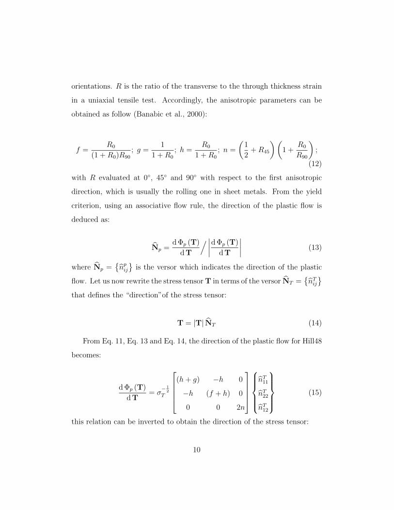
orientations. R is the ratio of the transverse to the through thickness strain
in a uniaxial tensile test. Accordingly, the anisotropic parameters can be
obtained as follow (Banabic et al., 2000):
f =R0
(1 +R0)R90
; g =1
1 +R0
; h =R0
1 +R0
; n =
(1
2+R45
)(1 +
R0
R90
);
(12)
with R evaluated at 0◦, 45◦ and 90◦ with respect to the first anisotropic
direction, which is usually the rolling one in sheet metals. From the yield
criterion, using an associative flow rule, the direction of the plastic flow is
deduced as:
Np =d Φp (T)
d T
/∣∣∣∣d Φp (T)
d T
∣∣∣∣ (13)
where Np ={npij}
is the versor which indicates the direction of the plastic
flow. Let us now rewrite the stress tensor T in terms of the versor NT ={nTij}
that defines the “direction”of the stress tensor:
T = |T| NT (14)
From Eq. 11, Eq. 13 and Eq. 14, the direction of the plastic flow for Hill48
becomes:
d Φp (T)
d T= σ
− 12
T
(h+ g) −h 0
−h (f + h) 0
0 0 2n
nT11
nT22
nT12
(15)
this relation can be inverted to obtain the direction of the stress tensor:
10

NT =A Np∣∣∣A Np
∣∣∣ (16)
with
A Np =
f + h h 0
h h+ g 0
0 0 gf+gh+hf2n
nP11
nP22
nP12
(17)
The versor of the stress tensor NT is directly derived from the direction
of the plastic flow Np. The modulus of the stress tensor |T| from the versor
NT can also be computed. Indeed, from Eq. 9 and Eq. 11:
σT (T) = σT
(|T| NT
)= |T|σT
(NT
)= σY (18)
and:
|T| = σY
[(g + h) nT11
2+ (f + h) nT22
2 − 2h nT11nT22 + 2n nT12
2]−1
2(19)
Then stress tensor T is obtained from Eq. 14.
The yield stress σY depends on the hardening law, which is usually a
function of the equivalent plastic strain. The procedure above, applied to
the Hill48 yield function, is general and can be adapted to any plasticity
model with a convex yield locus. For more in-depth insight on this, the
reader is referred to Rossi and Pierron (2012a).
The hardening law used here is Swift’s law expressed by:
σY = KH (p+ ε0)NH (20)
11

where σY is the yield stress, KH , ε0 and NH are the model parameters, and
p is the equivalent cumulated plastic strain. The equivalent plastic strain is
defined so that the plastic work can be expressed in terms of the equivalent
stress, that is:
∫ p(t)
p(0)
σY dp =
∫ Ep(t)
Ep(0)
T : dEp (21)
where Ep is the plastic strain tensor. Combining Eq. 9, Eq. 11 and Eq. 14,
the increment of plastic strain dp at time t can be obtained in terms of NT
and Np as:
dp =NT : Np
σT
(NT
) |dEp| (22)
The plastic flow direction can be defined as the direction of the plastic
strain rate tensor, i.e.:
Np = Epk• / |Ep
k•| (23)
Considering a sufficiently small strain increment, the plastic strain rate
at time t can be evaluated as:
Ep • =∂Ep
∂t≈ Ep(t) − Ep(t−1)
∆t=
∆Ep(t)
∆t(24)
where Ep is the plastic strain tensor. Since the plastic deformation is isochoric
in pressure-independent plasticity and, at large strains, the elastic part is
small compared to the plastic one, the plastic strain tensor Ep(t) can be
approximately reduced to the deviatoric part of the total strain tensor E(t):
12

Ep ≈ E− 13tr (E) I (25)
The total strain tensor is computed as the spatial logarithmic strain or
Henky strain tensor:
E = lnV (26)
where V is obtained by polar decomposition of the deformation gradient F:
F = VR (27)
and F is computed from the displacement field u:
F = Grad u (x0, t) + I (28)
The displacement u is measured by a full-field optical method during
the experiment. The displacements are computed at coordinates x0 in the
reference placement. This is what most commercial Digital Image Correlation
(DIC, Sutton et al., 2009) software do, which is the reason why the reference
placement has been considered here.
The strain tensor Ep however cannot be directly used to compute the
stress. The deformation is defined in the global coordinate system while the
plastic flow law and the yield function are written according to the material
coordinate system aligned with the anisotropy axes, see Eq. 11.
Let us denote R|mat the rotation tensor to rotate the global coordinate
system into the material one in the reference placement. In the deformed
13

x
y
1 12
2
x0
xα
α
B0Bt
Ref. placement
Coord. system: (x,y)
Stress: T1PK
Log. Strain: E=lnU
Def. placement
Coord. system: (x,y)
Stress: T
Log. Strain: E=lnV
Figure 1: Finite deformation of the specimen, reference and current placement, rotation
of the material axes and corresponding stress and strain tensors
configuration, the deformation tensor in the material coordinate system will
be obtained by:
Ep|mat = R|Tmat(RT Ep R ) R
∣∣mat
(29)
where R is the rotation tensor obtained in the polar decomposition of the
deformation gradient tensor F. The rotated strain tensor is used in Eqs. 23
and 24 to obtain the plastic flow versor Np. Then, Eqs. 14, 16 and 19 are
applied to derive the Cauchy stress tensor T|mat, which is still in the material
coordinate system. Finally, the Cauchy stress tensor is rotated back to global
coordinate system:
T = R|mat(R T|mat RT
)R|Tmat (30)
The stress tensor, written in the global coordinate system, is used to
14

obtain the 1st Piola-Kirchhoff tensor (Eq. 4), which will be used in the VFM
formulation of Eqs. 7 and 8. Figure 1 shows a schematic of the specimen in
the reference and deformed placements, and summarize the stress and strain
tensors that have to be considered in the various cases.
2.3. Implementation of the Yld2000-2D model
In this section, the steps to implement the Yld2000-2D model in the stress
computation routine are illustrated. This model will be used in Section 5 to
identify the properties of a stainless steel sheet metal. This will allow to make
a comparison with Hill48 in an actual case, showing some of the shortcomings
of Hill48.
The equivalent stress for the Yld2000-2D criterion is:
σT (T) =
[1
2
(|X ′1 −X ′2|
a+ |2X ′′2 +X ′′1 |
a+ |2X ′′1 +X ′′2 |
a)] 1a
(31)
where X ′1, X′2 and X ′′1 , X
′′2 are the principal values of the X′ and X′′ tensors
obtained from the Cauchy stress tensor T with the following transformation:
X′ = L′T
X′′ = L′′T(32)
with L′ and L′′:
L′ =
2α1
3−2α1
30
−2α2
32α2
30
0 0 α7
(33)
15

L′ =
8α5−2α3−2α6+2α4
9−4α6−4α4−4α5+α3
90
−4α3−4α5−4α4+α6
98α4−2α6−2α3+2α5
90
0 0 α8
(34)
and α1,...,8 are the parameters that have to be identified. In order to compute
the stress field, the same procedure as that described in Section 2.2 can be
employed, using Eq. 31 instead of Eq. 11. With an associated flow rule,
Eq. 13 is still valid:
Np =d Φp (T)
d T
/∣∣∣∣d Φp (T)
d T
∣∣∣∣However, the computation of Np is not straightforward because of the
transformation. All the steps to compute the derivatives are detailed by
Yoon et al. (2004). Afterwards, in order to compute the stress versor NT ,
Eq. 13 has to be inverted. In this case, this cannot be done directly as in
Eq. 16. However it can be easily achieved numerically by interpolation.
Apart from these changes, the procedure for Yld2000-2D remains the
same than the one described for Hill48.
2.4. Check of the plasticity occurrence
The procedure described above allows for computing the stress tensor if
the considered strain increment is plastic. Therefore, at each step t, a check
is performed to evaluate if the considered step is in the elastic or plastic
domain
First, a trial stress Ttrial(t) is obtained assuming that the increment is
purely elastic. Then, the yield criterion (Eq. 10) and the hardening law
16

(Eq. 20) are used to check if the element undergoes plastic deformation.
Two cases are possible:
1. the element remains in the elastic domain
σT
(Ttrial
(t))− σY
(p(t−1)
)< 0
then
T(t) = Ttrial(t)
p(t) = p(t−1)k
2. the element is in the plastic domain
σT
(Ttrial(t)
)− σY
(p(t−1)
)> 0
then
T(t) computed from the routine of Sec. 2.2
p(t)k = p(t−1) + ∆p(t)
The current increment of plastic strain ∆p(t) is computed using Eq. 22.
The procedure is valid both for loading and unloading. If, within the same
increment, some part is elastic and some plastic, as for instance when the
first yielding occurs, the increment is subdivided in elastic and plastic parts.
2.5. Definition of the virtual fields
The optimal selection of virtual fields (VFs) for elasto-plasticity is still
an open question. In elasticity, the most used system to generate optimised
virtual fields was proposed byAvril et al. (2004): according to this method,
special virtual fields are automatically generated in order to minimize the
sensitivity to noise. Pierron et al. (2010) also applied a similar approach in
plasticity but with a relative success only. Indeed, in plasticity, the level of
17

deformation is usually much larger than in elasticity and the noise-to-signal
ratio is small. This means that noise sensitivity is most relevant optimisation
criterion to define virtual fields and other strategies have to be considered.
Here, the virtual fields have been selected empirically based on previous
experience from the authors. The problem of automatic definition of op-
timized virtual fields is still an outstanding problem in the Virtual Fields
Method, however, progress on this is expected soon and will be released in a
future publication. This is of particular importance for anisotropic plasticity
where the relative contribution of the different stress components to the cost
function is of primary interest. Here, the following virtual fields were defined,
as a first attempt to include all stress components in the cost function:
δv(1) =
δvx = 0
δvy =y
H
δv(2) =
δvx =
x
W
(|y| −H)
H
δvy = 0
δv(3) =
{δvx = δvy = 1
πsin(π xW
)cos(π y
2H
)
(35)
H and W are the height and the width of the specimen area where the VFM
is defined. When y = ±H, δvx = 0 and δvy is constant (δv(1)) or zero (δv(2)
and δv(3)). Such condition allows simplifying the second integral of Eq. 7 so
that only the resultant of the forces in the y-direction, i.e. the load measured
during the test by the load cell, is used to compute the external virtual work.
18
δ vx(1)
0
0.5
1δ v
y(1)
−0.500.5
δ vx(2)
−0.500.5
δ vy(2)
0
0.5
1
δ vx(3)
−0.200.2
δ vy(3)
−0.200.2
H
Wx
y
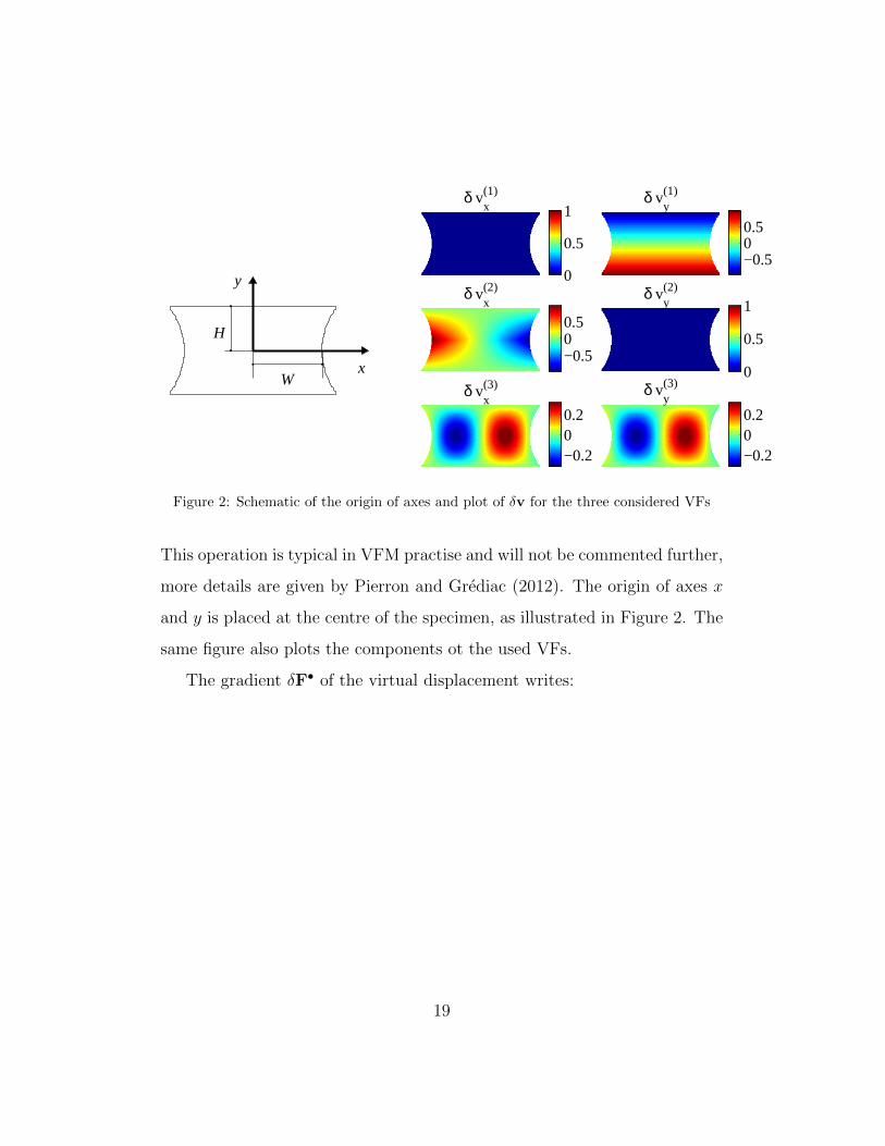
Figure 2: Schematic of the origin of axes and plot of δv for the three considered VFs
This operation is typical in VFM practise and will not be commented further,
more details are given by Pierron and Grediac (2012). The origin of axes x
and y is placed at the centre of the specimen, as illustrated in Figure 2. The
same figure also plots the components ot the used VFs.
The gradient δF• of the virtual displacement writes:
19

δF• (1) =
0 0
01
H
δF• (2) =
(|y| −H)
WHsgn (y)
x
WH
0 0
δF• (3) =
1W
cos(π xW
)cos(π y
2H
)− 1
2Hsin(π xW
)sin(π y
2H
)1W
cos(π xW
)cos(π y
2H
)− 1
2Hsin(π xW
)sin(π y
2H
)
(36)
∂ ( δ vx ) / ∂ x
0
0.5
1
∂ ( δ vx ) / ∂ y
0
0.5
1
∂ ( δ vy ) / ∂ x
0
0.5
1
∂ ( δ vy ) / ∂ y
0
0.02
−0.03−0.02−0.01
−0.0500.05
0
0.5
1
0
0.5
1
−0.0200.02
−0.0200.02
−0.0200.02
−0.0200.02
1st
VF
2nd
VF
3rd
VF
Figure 3: Plot of the components of δF• for the three considered VFs
In order to compute the internal virtual work (first integral of Eq. 7),
each component of Piola-Kirchhoff stress tensor T1PK is multiplied by the
corresponding component of δF•. Using the 1st VF, only T 1PKyy , that is the
stress component in the loading direction, is considered in the internal virtual
20

work. The 2nd VF, instead, involves T 1PKxx and T 1PK
xy . The 3rd VF, finally,
has all non-zero components, therefore it activates all the four components
of T1PK .
A graphical representation of the three VFs is provided in Figure 3, the
contour maps shows that the average value is similar for the different VFs,
so that, when they are used together in Eq. 8, their relative weight is com-
parable.
3. Numerical validation
The numerical validation was performed using FE simulations that repro-
duce a tensile test on notched specimens, using the Hill48 criterion. Figure 4a
illustrates the geometry of the specimen, which is the same as that used in
the experiments. The notched shape is often used because it is able to pro-
duce an heterogeneous strain field, is easy to machine, and, in plasticity,
allows to have a large zone of the specimen under plastic deformation. This
is particularly valuable looking at large strains, while for instance Σ−shaped
specimens, like the ones proposed by Kim et al. (2014), localize the strain in
a small area and leaves the majority of the specimen at low deformations.
However, the design of an optimized specimen is still an open problem. Re-
cent advances in test specimen design for orthotropic elasticity have been
published (Gu and Pierron, 2016) based on a simulator which reproduces the
whole identification process, also taking into account the systematic errors
caused by the DIC measurements. Extension of this to elasto-plasticity is
on the way, although this will be greatly computationally expensive as many
identification problems need to be solved in the process. In any case, this is
21

beyond the scope of the present paper.
In the future optimization methods could be adopted to find out the best
geometry, as done for instance by Wang et al. (2016) for polymeric foams or
by Rossi and Pierron (2012b) for orthotropic composite materials.
The element orientation can be varied with respect to the loading di-
rection, in order to reproduce specimens cut in different directions. As a
convention, angle α measures the rotation between the rolling and the load-
ing direction. The global coordinate system is denoted {x, y}, where y is the
loading direction, while the local coordinate system is denoted {1, 2}, where
1 represents the rolling direction.
The FE model illustrated in Figure 4b was built up with ABAQUS stan-
dard, using CPS4 elements (four nodes, bilinear shape functions, full inte-
gration) and large displacement formulation. A total displacment of 30 mm
(10% of the specimen’s length) was applied to one end of the specimen. Fig-
ure 4b shows the used mesh and a contour plot of the equivalent plastic
strain at the last increment of the test, which is around 0.5. The contour
map indicates that the deformation field, and accordingly the stress field, is
heterogeneous thanks to the round notches at the sides of the specimen.
The nature of the generated stress field can be better depicted in the
graph of Figure 5, which plots a 2D view of the yield surface. In this type of
graphs, used for instance by Barlat et al. (2003), the horizontal and vertical
axes represent the σ11 and σ22 stress components, normalized according to
the equivalent stress. The 3rd axis, perpendicular to the figure plane, repre-
sents the normalized shear stress σ12. The anisotropic yield surface can be
therefore represented as contour lines, where the external line represent the
22

R 25
100
50
300
α
Loading
direction
Rolling
directionTransverse
direction
1
2
(a) Geometry
(Avg: 75%)PEEQ
0.0000.0380.0760.1130.1510.1890.2270.2640.3020.3400.3780.4150.453
Number of nodes: 4361Number of elements: 4200Element type: CPS4
(b) FEM
Figure 4: Specimen geometry (units: mm) and corresponding FE model. The equivalent
plastic strain map is shown for an end’s displacement of 30 mm (α = 0◦)
23

yield surface when the shear stress σ12 = 0 and the origin is the condition of
pure shear.
−0.5 0 0.5 1 1.5−0.5
0
0.5
1
1.5
σ11
/ σeq
σ 22 /
σ eq
α=0°
α=45°
α=90°
σ12
= 0
σ12
/σeq
= 0.5
Figure 5: Distribution of the stress
In this chart, each point represents a different state of stress. Since the
stress is normalized, all points of all time steps can be introduced in the
same graph. A practical recommendation of the VFM is that the specimen
should produce a sufficiently heterogeneous state of stress, so that different
stress conditions can be evaluated at the same time. With the adopted con-
figuration, using a single specimen, only a small part of the yield surface
can be covered, as illustrated in Figure 5. For instance, using a specimen
with α = 0◦, only the zone close to uniaxial tensile tension in the 1st direc-
tion is covered. Also, even when using notched specimens at three different
orientations, the pure shear and the biaxial conditions cannot be reached.
24

As a first numerical check, the VFM was applied to the strain maps
generated with the FEM computations without any noise. In order to check
the stress reconstruction algorithm described in Section 2.2, Figure 6 shows
a comparison between the Cauchy stress tensor computed by FEM and the
one obtained from the displacement field using the proposed method. A good
agreement is found.
σxx
FEM
50
100
150
200
σyy
FEM
400
450
500
550
σxy
FEM
−200
−100
0
100
200
σxx
Computed σyy
Computed σxy
Computed
Difference
−5
0
5Difference
−10
−6
−2Difference
−5
0
5
Figure 6: Comparison between the FEM and computed stress components using the re-
construction routine
The results of the identification with the VFM are summarized in Ta-
ble 1. The combination of 3 VFs always improves the identification. Using
a single specimen at 0◦, R90 cannot be identified and conversely for R0 with
25

a specimen at 90◦.
The specimen cut at 45◦ however allows to correctly identify all param-
eters, with an error lower than 1%, when the three VFs are used. Similar
results are obtained introducing both 0◦ and 90◦ specimens in the cost func-
tion. These results can be explained looking at the graph of Figure 5, the
45◦ specimen covers a larger part of the yield surface and allows looking at
both anisotropy directions. The same result can be obtained combining the
0◦ and 90◦ specimen.
∆εxx
−0.012
−0.01
−0.008
−0.006
−0.004
−0.002
0
∆εyy
0
0.002
0.004
0.006
0.008
0.01
0.012
0.014
∆εxx
−0.015
−0.01
−0.005
0
0.005
0.01
0.015
Nois
e st
d:
1⋅1
0−
3
no s
mooth
ing
Nois
e st
d:
5⋅1
0−
3
no s
mooth
ing
Nois
e st
d:
5⋅1
0−
3
smooth
ing
Figure 7: Strain increment fields with noise, without and with temporal smoothing
A second validation was conducted to evaluate the effect of noise. Dealing
with large deformation, noise has a minor impact on identification, however,
in order to define the direction of the plastic flow, the strain increment ∆E
is used in Eq. 24. This value can be small enough so that noise plays a role.
Two levels of noise were considered with a standard deviation of 10−3 and
5 · 10−3, respectively. The first represents a rather large strain uncertainty
26

Specimen Virtual Fields identified parameters
configurations K ε0 N R0 R45 R90
Reference 1000 0.02 0.5 1.8 1.1 2.5
0◦ V F1 1208.5 0.0171 0.4799 0.58 0.33 0.47
Error -20.85% 14.52% 4.02% 67.56% 70.04% 81.32%
V F1 + V F2 1010.2 0.0169 0.4812 1.93 1.05 1.20
Error -1.02% 15.46% 3.77% -7.44% 4.67% 52.00%
V F1 + V F2 + V F3 1017.1 0.0176 0.4871 1.79 1.17 1.47
Error -1.71% 12.19% 2.58% 0.65% -6.72% 41.17%
90◦ V F1 1048.8 0.0188 0.5049 2.17 1.61 2.38
Error -4.88% 6.03% -0.98% -20.49% -46.55% 4.98%
V F1 + V F2 975.6 0.0201 0.5030 1.74 1.01 2.62
Error 2.44% -0.48% -0.61% 3.49% 8.37% -4.61%
V F1 + V F2 + V F3 702.0 0.0207 0.4714 0.62 1.07 2.58
Error 29.80% -3.38% 5.72% 65.63% 2.94% -3.14%
45◦ V F1 906.0 0.0198 0.4982 2.32 1.21 3.00
Error 9.40% 0.78% 0.36% -29.14% -10.30% -20.00%
V F1 + V F2 1014.7 0.0198 0.5035 1.57 1.12 2.59
Error -1.47% 1.10% -0.70% 12.96% -1.97% -3.58%
V F1 + V F2 + V F3 994.5 0.0197 0.5016 1.80 1.09 2.50
Error 0.55% 1.49% -0.32% 0.21% 1.00% -0.15
0◦ + 90◦ V F1 992.9 0.0189 0.4987 1.79 1.47 2.47
Error 0.71% 5.66% 0.25% 0.79% -33.74% 1.30%
V F1 + V F2 995.7 0.0200 0.5047 1.84 1.03 2.56
Error 0.43% 0.01% -0.94% -2.23% 6.59% -2.51%
V F1 + V F2 + V F3 1005.3 0.0196 0.5029 1.77 1.11 2.45
Error -0.53% 1.79% -0.59% 1.41% -0.84% 2.01%
Table 1: Results of the numerical validation, different combination of VFs and specimen
orientations are considered
27

for DIC measurements (Sutton et al., 2009), the second a severe (unrealistic)
noise condition. Noise was directly applied as a random number to the strain
field. For the higher noise condition, temporal smoothing (Le Louedec et al.,
2013) was introduced to reduce the noise effect, as illustrated in Figure 14.
Temporal smoothing was performed by computing the strain rate at time
t using more time steps and performing a polynomial fitting. This can be
efficiently implemented using a convolution method as the one provided by
Savitzky and Golay (1964).
The strain rate of Eq. 24 can be rewritten as:
Ep • =∂Ep
∂t≈
m∑j=−m
hjEp(t+m)
∆t(37)
thus, the strain rate at the time t is computed using 2m+1 steps. A procedure
to compute the convolution weights hj is given by Gorry (1990), the method
allows considering also the end points of the data set. In the present case,
the smoothing was performed using 7 points (m = 3).
Table 2 shows the parameters identified for the different cases. With the
low noise level, all parameters are identified with a good confidence, even
if no smoothing is applied. With the high noise level, the identification is
not correct, with errors over 10% for most of the identified parameters. As
expected, looking at the anisotropy parameter R, using the 45◦ specimen
a poor identification is obtained for R0 and R90; combining the 0◦ and 90◦
specimens, a larger error is obtained for R45. With temporal smoothing,
a correct identification is obtained for all parameters except ε0. However,
this parameter, used in Eq. 20, has a marginal impact in the definition of
28

Specimen Noise Identified Parameters
configurations standard
deviation K ε0 N R0 R45 R90
Reference 1000 0.02 0.5 1.8 1.1 2.5
45◦ 1 · 10−3 983.7 0.0188 0.4966 1.88 1.08 2.50
Error 1.63% 5.92% 0.67% -4.69% 1.80% 0.16%
5 · 10−3 807.8 0.0022 0.4065 3.00 1.00 2.96
Error 19.22% 89.13% 18.70% -66.67% 8.72% -18.48%
5 · 10−3 smoothed 974.9 0.0277 0.5018 1.80 1.09 2.62
Error 2.51% -38.50% -0.37% -0.09% 1.21% -4.76%
0◦ + 90◦ 1 · 10−3 999.6 0.0184 0.4951 1.78 1.12 2.45
Error 0.04% 8.04% 0.98% 1.15% -1.64% 1.81%
5 · 10−3 918.0 0.0001 0.3714 1.80 1.31 2.48
Error 8.20% 99.50% 25.72% -0.18% -19.20% 0.68%
5 · 10−3 smoothed 1002.4 0.0295 0.5079 1.78 1.13 2.46
Error -0.24% -47.68% -1.59% 1.09% -2.73% 1.73%
Table 2: Influence of noise on VFM identification
the hardening law (Rossi and Pierron, 2012a). Therefore its variation does
not introduce significant modification in the identified true stress-true strain
curve.
The main outcomes of the numerical validation can be summarized as
follow:
• the effectiveness of the VFM depends on the heterogeneity of the stress
field. The spread of stress distribution can be visualized conveniently
in a normalized stress plane (Figure 5);
• the adopted notched specimens generate a state of stress that spans
29

Specimen Virtual Fields Iter. Ψ eval. CPU time Ψ av. time
configuration [s] [s]
0◦ V F1 74 604 1335 2.2
V F1 + V F2 74 606 1333 2.2
V F1 + V F2 + V F3 76 602 1328 2.2
0◦ + 90◦ V F1 55 538 2367 4.4
V F1 + V F2 55 537 2362 4.4
V F1 + V F2 + V F3 56 519 2284 4.4
Table 3: CPU time used to perform the identification
only a small part of the yield surface. However, for the Hill48 crite-
rion, good identification can be obtained using a 45◦ specimen or the
combination of 90◦ and 0◦;
• the combination of three virtual fields allows reducing the identification
error;
• strain noise does not represent a major problem. In case of severe noise,
temporal smoothing applied to the strain field significantly increases
the quality of the identification.
3.1. Computational time
In the eventuality of using an inverse identification method at the indus-
trial level, the computational time becomes an important aspect that should
be taken into consideration. One advantage of the VFM is that the identifica-
tion routine is rather fast compared to, for instance, finite element updating,
where an FE model has to be run for each iteration.
30

Table 3 shows the time required to perform the identification. The anal-
ysis was performed with a standard computer (Intel R© CoreTM 2 CPU 6700
@ 2.66GHz 2.66GHz, RAM: 4.00 GB) using non-optimized Matlab routines.
The time required for a single iteration is about 2.2 s when a single test is
considered. This is more or less constant regardless of the number of virtual
fields used in the cost function. The time for a cost function evaluation
is however doubled when a second test is introduced because of the stress
reconstruction. On the other hand, when two tests are used, the number
of iterations required to identify the parameters is reduced from 74 − 76 to
55−56. Therefore the overall CPU time needed to perform the identification
is less than double compared to the identification with a single test.
This computational time could be definitely reduced using faster pro-
gramming languages and higher CPU speed, showing the potentiality of this
method to be used in industrial applications, where time is an important
added value.
4. Experiments
The experiments were conducted on notched specimens with the same
geometry used in the numerical validation, and illustrated in Figure 4a. The
specimens were cut from a blank sheet of stainless steel, 0.75 mm thick. Three
different cutting directions were used: 0◦, 45◦ and 90◦. The yield stress and
the Lankford parameter measured in the three directions by standard uniaxal
31

Dir. Thick. Rp0.2 Rm A80 Ag R
3% 5% 10% 15% 20%
mm MPa MPa % %
0◦ 0.75 128 296 45 25 1.8 1.9 1.9 1.9 1.9
45◦ 0.75 138 305 43 24 1.5 1.5 1.5 1.6 1.6
90◦ 0.75 132 294 44 25 2.1 2.1 2.2 2.2 2.3
Table 4: Results of uniaxial test according to EN 10002-1 for three directions . R is
evaluated at different levels of engineering strain
tests, according to the EN 10002-1 standard2, are listed in Table 4.
The full-field displacement field was obtained by stereo Digital Image Cor-
relation (DIC), using the commercial software VIC-3D. We used black and
white sprays to create the speckle pattern onto the specimen surface (white
background and black speckles). The thickness of the paint was kept thin so
that it was able to undergo large deformation without flaking. An example
of the speckle pattern obtained during the test is illustrated in Figure 9. It
is able to follow the deformation of the specimen up to the final fracture.
The experimental set-up is illustrated in Figure 8. An INSTRON-880
tensile machine with hydraulic grips was used to perform the tests. The
cameras are two JAI Pulnix TM-4000CL. Table 5 summarizes the information
about the sensor, the camera noise, the DIC settings and the displacement
and strain resolution.
2Rp0.2 = 0.2 % offset yield strength; Rm = tensile strength at maximum force;
A80 = percentage elongation after fracture; Ag = Percentage elongation at maximum
force.
32
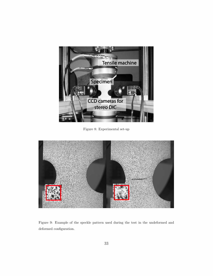
Figure 8: Experimental set-up
Figure 9: Example of the speckle pattern used during the test in the undeformed and
deformed configuration.
33

Technique used Stereo digital image correlation
Sensor and digitization 2048 × 2048, 10-bit
Camera noise (% of range) 0.6 %
Pixel to mm conversion 1 pixel = 0.055 mm
ROI (mm) 100 mm × 80 mm
Subset, step 27, 5
Interpolation, shape functions, bilinear, affine
Correlation criterion ZNSSD
Pre-smoothing Gaussian 5
Displacement resolution 0.01 pixels, 0.55 µm
Strain derivation 2nd order polynomial fitting
Strain window 5× 5
Strain resolution 2.5 · 10−4
Table 5: Sensor characteristics, DIC settings, displacement and strain resolution.
The correlation algorithm was run using a subset window of 27 pixels and
a step of 5 pixels between two measurement points. The incremental correla-
tion options was used, i.e. each image is correlated with the previous one and
the measured incremental displacement is added to the one measured in the
previous step. Figure 10 shows an example of displacement fields obtained
from the experiments, the red box highlights the zone of the specimen used
subsequently for the VFM. In this zone, with the adopted settings, 101×216
measurement points were obtained for each step.
The VFM was restricted to this smaller zone for two reasons: first, it re-
mains planar up to large strains whereas the external parts of the specimen
34

tend to wrinkle as the deformation increases; secondly, the plastic flow local-
izes within this zone while the external parts mainly remains in the elastic
regime. In the future, however, the geometry and the experimental set-up
should be modified to better exploit the spatial resolution of the stereo-DIC
measurement.
x coord
y co
ord
Ux
−50 0 50−40
−20
0
20
40
−0.4
−0.2
0
0.2
0.4
0.6
x coord
y co
ord
Uy
−50 0 50−40
−20
0
20
40
−4
−3
−2
−1
Figure 10: Displacement field measured by stereo DIC, the zone used to perform the
identification is highlighted by the red box
Stereo DIC allows recording out-of-plane movements, which can be caused
by misalignments of the camera with respect to the specimen surface or by
instabilities (buckling, wrinkling, etc.) of the sheet metal during deformation.
In this case, plastic instabilities occurs in all specimens at the final stage of
the test. Figure 11 shows the onset of instability in terms of out of plane
displacement. Nonetheless, 48 time steps were recoreded before the onset of
instability and used to perform the VFM identification. At the final available
step, the maximum engineering strain was around 20%, which is already in
the large plasticity region. In the future, in order to investigate larger strains,
35

x coord
y co
ord
−50 0 50−40
−20
0
20
40
−4
−3
−2
−1
0
1
Figure 11: Out of plane movements measured after the onset of plastic instability
the shape of the specimen should be optimized to avoid, or postpone, the
instability.
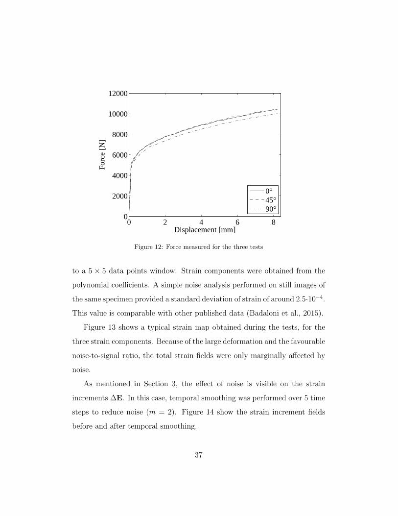
The cameras were synchronized with the load cell so that, for each image,
the system records the corresponding tensile force. The measured force versus
displacement curves are plotted in Figure 12. The variation between the tests
is due to the anisotropic behaviour of the material.
5. Results and discussion
In the following section, the parameter identification performed with the
VFM from the experimental data is discussed.
5.1. Application of the Hill48 criterion
First, the VFM was used with the experimental data in order to identify
the parameters of the Hill48 model. The logarithmic strain E (Eq. 26) at each
step was computed from the measured displacement field. Spatial smoothing
was used before differentiation by fitting the best second order polynomial
36
0 2 4 6 80
2000
4000
6000
8000
10000
12000
Displacement [mm]
For
ce [N
]
0°45°90°
Figure 12: Force measured for the three tests
to a 5 × 5 data points window. Strain components were obtained from the
polynomial coefficients. A simple noise analysis performed on still images of
the same specimen provided a standard deviation of strain of around 2.5·10−4.
This value is comparable with other published data (Badaloni et al., 2015).
Figure 13 shows a typical strain map obtained during the tests, for the
three strain components. Because of the large deformation and the favourable
noise-to-signal ratio, the total strain fields were only marginally affected by
noise.
As mentioned in Section 3, the effect of noise is visible on the strain
increments ∆E. In this case, temporal smoothing was performed over 5 time
steps to reduce noise (m = 2). Figure 14 show the strain increment fields
before and after temporal smoothing.
37

εxx
−0.10
−0.05
−0.01
εyy
0.04
0.08
0.13
γxy
−0.11
0.01
0.13
Figure 13: Example of strain fields obtained from the stereo DIC measurement (Force:
9.7 kN, direction: 90◦)
−3
−2.5
−2
−1.5
−1
−0.5
x 10−3
1
1.5
2
2.5
3
3.5x 10
−3
−2
−1
0
1
2
3
x 10−3
No
tem
po
ral
smo
oth
ing
Tem
po
ral
smo
oth
ing
Figure 14: Experimental strain increments, with and without temporal smoothing (Force:
9.7 kN, direction: 90◦)
38

Specimen Identified parameters Cost function
configuration K ε0 N R0 R45 R90
0◦ 1183 0.035 0.64 1.76 0.94 0.3 192
90◦ 439 0.012 0.43 0.46 0.77 2.20 207
45◦ 888 0.012 0.43 1.10 1.35 0.78 115
0◦ + 90◦ 665 0.010 0.41 1.95 0.78 1.82 423
0◦ + 45◦ + 90◦ 735 0.010 0.41 1.21 1.32 1.12 576
Reference - - - 1.88 1.56 2.18
Table 6: Experimental results
Table 6 reports the identified parameters and the reference R values ob-
tained from the standard uniaxial tests, see Table 4. In this case, the hard-
ening parameters, K, ε0 and N , cannot be directly compared with reference
experimental values. However, a comparison with the experiments can be
performed in terms of tensile force. The load Li, measured experimentally
at each step i, can be indeed compared with the force computed using the
identified parameters and the measured strain field. Following the definition
of VF1 (Eq. 35):
∫∂B0
(T1PKn0
)· δv(1) da0 = 2Li (38)
and, from Eq. 3:
Li =1
2
∫B0
T1PKi · δF• (1) dv0 (39)
where T1PKi
(ξ, u|0→t
)is obtained from the measured displacement field us-
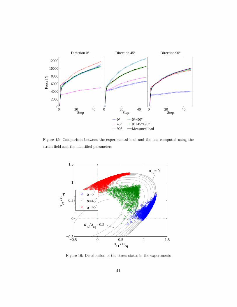
ing the identified constitutive parameters ξ. Figure 15 shows the comparison
39

between the measured force and the force reconstructed from the strain and
the material model, for all time steps (horizontal axis). As expected, using
a single test at 0◦ or 90◦, the parameters of the corresponding directions are
correctly identified while a large error is encountered for the other directions.
Using the specimen at 45◦, the error diminished but the load in the 0◦ direc-
tion is still not reproduced correctly. Using 0◦ + 90◦, the load at 45◦ is not
reproduced correctly. When all tests in the three directions are used in the
cost function, the force is correctly reproduced in all cases.
The identification of R in the different directions is more critical: looking
at Table 6, using a single direction, the R values are similar to the experi-
mental reference only for the corresponding directions. Using 0◦ + 90◦, R45
is not well identified. When all specimens are used, all values of R are rather
different from the reference.
The reason for this is that, in this case, the Hill48 model is not able to
reproduce the behaviour of the material. When the cost function is con-
strained with all tests, the VFM identifies the best set of parameters for the
Hill48 model, which is however not able to describe the material behaviour.
The cost function (Ψ), obtained at the end of the minimization, can be
considered an indicator of the quality of the identification (Rossi et al., 2014).
In this case, the cost function is larger when all three tests are considered.
This suggests that, when more tests are used at the same time, the mini-
mization algorithm is not able to reduce the error beyond a certain limit.
Figure 16 illustrates the stress states mapped onto the yield surface for the
experiments. The map is very similar to the one obtained for the numerical
case (Figure 5), and shows the zone of the yield function covered by the
40
0 20 400
2000
4000
6000
8000
10000
12000
Step
For
ce [N
]
Direction 0°
0 20 40Step
Direction 45°
0°45°90°
0 20 40Step
Direction 90°
0°+90°0°+45°+90°Measured load
Figure 15: Comparison between the experimental load and the one computed using the
strain field and the identified parameters
−0.5 0 0.5 1 1.5−0.5
0
0.5
1
1.5
σ11
/ σeq
σ 22 /
σ eq
α=0°
α=45°
α=90°
σ12
/σeq
= 0.5
σ12
= 0
Figure 16: Distribution of the stress states in the experiments
41

performed experiments.
5.2. Application of the Yld2000-2D criterion
The Hill48 criterion is not able to reproduce the behaviour of the tested
material. In order to support this statement, the same VFM approach was
employed to identify the parameters of the Yld2000-2D model (Barlat et al.,
2003).
In this case 11 parameters have to be identified from the minimization
algorithm, 3 for the hardening law and 8 for the yield function. This model
is more versatile than Hill48, where only 3 parameters are used to describe
the anisotropy.
The identification was conducted using the three tests (0◦ + 45◦ + 90◦)
and the same three VFs used for Hill48. As first guess, the Yld2000-2D
parameters are set equal to 1 (α1,...,8 = 1), while the hardening parameters
(K , ε0, N) are set equal to the ones identified with the Hill48 criterion.
In spite of the rather large number of parameters, the minimization al-
gorithm was able to converge to a set of parameters as listed in Table 7. In
order to check the stability of the identified parameters, different initial con-
ditions were tested. Two sets of parameters were generated randomly and
used as first guess in the minimization algorithm. The results obtained with
the different sets of initial guess are compared in Table 8. A slight variation
is observed in the hardening parameters, while the anisotropic parameters αi
are not sensitive to the initial guess. Thus, the identification procedure can
be considered sufficiently stable.
Figure 17 shows the distribution of the stress states in the identified yield
function. Figure 18 shows the comparison of the two models in terms of
42

Hardening Yld2000-2D parameters
K ε0 N α1 α2 α3 α4 α5 α6 α7 α8
852 0.01 0.41 1.11 1.35 1.21 1.11 1.07 0.96 1.21 1.15
Table 7: Parameters identified from the experimental tests using Yld2000-2D
Initial guess
K ε0 N α1 α2 α3 α4 α5 α6 α7 α8
set 1 735 0.01 0.41 1.00 1.00 1.00 1.00 1.00 1.00 1.00 1.00
set 2 1240 0.015 0.3 1.55 1.60 1.48 1.83 1.23 1.01 1.94 0.68
set 3 520 0.05 0.7 1.54 1.16 1.12 0.72 1.31 0.79 1.62 1.57
Identified parameters after minimization
K ε0 N α1 α2 α3 α4 α5 α6 α7 α8
set 1 852 0.01 0.41 1.11 1.35 1.21 1.11 1.07 0.96 1.21 1.15
set 2 910 0.01 0.42 1.11 1.34 1.20 1.10 1.07 0.95 1.20 1.15
set 3 805 0.01 0.39 1.10 1.36 1.22 1.10 1.07 0.95 1.21 1.14
Table 8: Influence of initial guess in the minimization process, set 2 and set 3 were obtained
using random numbers.
43

0 0.5 1
0
0.5
1
σ11
/ σeq
σ 22 /
σ eq
α=0°
α=45°
α=90°
σ12
/σeq
= 0.5
σ12
= 0
Figure 17: Distribution of the stress states and yield surface using Yld2000-2D
computed tensile force, as in Figure 15. Both models are able to reproduce
the experimental force. This shows that such a macroscopic information is
not enough to discriminate between models. Table 9 presents the results in
terms of Lankford parameter R. In this case, the Yld2000-2D model gives
values that are much closer to the experimental ones, obtained from the
uniaxial tests. Looking at the cost function for the Yld2000-2D model, it is
more than 3 times lower than for the Hill48 model.
It is beyond the scope of this paper to give a complete validation for the
Yld2000-2D model, as done for the Hill48 model. This will be the object of
future work. However, this simple verification is useful to demonstrate the
potentiality of the adopted approach. Another important question, which
should be investigated in the future, is if the parameters identified with the
44

0 10 20 30 40 500
2000
4000
6000
8000
10000
12000
14000
Step
For
ce [N
]
Direction 0°
0 10 20 30 40 50Step
Direction 45°
0 10 20 30 40 50Step
Direction 90°
Measured loadHILL48YLD2000−2D
Figure 18: Force comparison with Hill48 and Yld2000-2D
R0 R45 R90 Cost function
Hill48 1.21 1.32 1.12 576
Yld2000-2D 2.00 1.63 2.07 153
Reference 1.88 1.54 2.18
Table 9: Comparison of R values between Hill48 and Yld2000-2D models.
45

notched specimens are able to predict the plastic behaviour in the biaxial
condition. This can be done using a bulge test or a disc compression test,
as showed for instance by Tardif and Kyriakides (2012) for the Yld2004-3D
model.
6. Conclusion
This paper describes an application of VFM to large strain anisotropic
plasticity. A numerical validation was first performed using simulated tests
generated according to the Hill48 yield criterion. The procedure led to the
identification of the constitutive parameters with a good accuracy using a
single test, namely a notched specimen cut at 45◦ respect to the rolling di-
rection. Then experiments were performed on a stainless steel sheet, using
the same specimen geometry. In this case, although the hardening behaviour
is well characterized, the procedure was not able to identify the R-values in
the different directions. Moreover, in order to have reasonable results, all
directions have to be included in the minimization function. Such behaviour
can be explained from the fact that the material does not follow the Hill48
model. The VFM provides the Hill48 parameters that best fit the experimen-
tal data but these do not match the uniaxial ones. A correct identification
of R can be achieved using the Yld2000-2D model.
From this study, the following main outcomes can be listed:
• the experiment should be designed so that, during the test, the stress
states in different points of the specimen cover the largest part of the
yield surface. In the present application, a notched specimen was used,
46

which produced a rather heterogeneous stress/strain field during defor-
mation. Although satisfactory results were obtained with this geome-
try, we believe that the specimen design could be improved and further
studies are needed in this sense;
• if the material follows the Hill48 plasticity model, a single test is suffi-
cient to correctly identify the parameters; noise can be easily handled
with temporal smoothing;
• if the material does not follow the assumed plasticity model, as for
the experimental case and the Hill48 model, the method provides the
parameters that best fit the experimental behaviour. However, the
more heterogeneous the test is, the more difficult it is to find a good
compromise. In this case a single test is no more sufficient to identify
the parameters;
• the VFM cost function can be used as a benchmark indicator to com-
pare the performance of different constitutive models.
As a general remark, the VFM is an effective tool to study the plastic
behaviour of materials at large strains. Full-field data can be processed with
low computational times to identify the constitutive parameters of plastic-
ity models. In the future, a more thorough study of the influence of DIC
parameters (step size, subset size, virtual strain gauge, etc.) on the iden-
tification should be performed, as done by Rossi et al. (2015) for elasticity.
More complex constitutive models should be introduced and other specimen
shapes should be tested.
47

Avril, S., Grediac, M., Pierron, F., 2004. Sensitivity of the virtual fields
method to noisy data. Comput. Mech. 34 (6), 439–452.
Avril, S., Pierron, F., Pannier, Y., Rotinat, R., 2008. Stress reconstruc-
tion and constitutive parameter identification in plane-stress elasto-plastic
problems using surface measurements of deformation fields. Experimental
Mechanics 48 (4), 403–419.
Badaloni, M., Rossi, M., Chiappini, G., Lava, P., Debruyne, D., 2015. Impact
of experimental uncertainties on the identification of mechanical material
properties using DIC. Exp. Mech. Accepted.
Bai, Y., Wierzbicki, T., 2008. A new model of metal plasticity and fracture
with pressure and Lode dependence. Int. J. Plasticity 24 (6), 1071–1096.
Banabic, D., Bunge, H.-J., Pohlandt, Tekkaya, A., 2000. Formability of
metallic materials. Springer Berlin.
Barlat, F., Brem, J., Yoon, J., Chung, K., Dick, R., Lege, D., Pourboghrat,
F., Choi, S.-H., Chu, E., 2003. Plane stress yield function for aluminum
alloy sheets - Part 1: Theory. Int. J. Plasticity 19 (9), 1297–1319.
Barlat, F., Lege, D., Brem, J., 1991. A six-component yield function for
anisotropic materials. Int. J. Plasticity 7 (7), 693–712.
Cazacu, O., Plunkett, B., Barlat, F., 2006. Orthotropic yield criterion for
hexagonal closed packed metals. Int. J. Plasticity 22, 1171–1194.
Cooreman, S., Lecompte, D., Sol, H., Vantomme, J., Debruyne, D., 2008.
48

Identification of mechanical material behavior through inverse modeling
and dic. Exp. Mech. 48 (4), 421–433.
Coppieters, S., Cooreman, S., Sol, H., Van Houtte, P., Debruyne, D., 2011.
Identification of the post-necking hardening behaviour of sheet metal by
comparison of the internal and external work in the necking zone. J Mater.
Process. Tech. 211 (3), 545–552.
Coppieters, S., Kuwabara, T., 2014. Identification of post-necking hardening
phenomena in ductile sheet metal. Exp. Mech. 54 (8), 1355–1371.
Cortese, L., Coppola, T., Campanelli, F., Campana, F., Sasso, M., 2014.
Prediction of ductile failure in materials for onshore and offshore pipeline
applications. Int. J. Damage Mech. 23 (1), 104–123.
Darrieulat, M., Piot, D., 1996. A method of generating analytical yield sur-
faces of crystalline materials. Int. J. Plasticity 12, 575–610.
Feigenbaum, H. P., Dafalias, Y. F., 2007. Directional distortional hardening
in metal plasticity within thermodynamics. Int. J. Solids Struct. 44, 7526–
7542.
Gorry, A., 1990. General least-squares smoothing and differentiation by the
convolution (Savitzky-Golay) method. Anal. Chem. 62, 570–573.
Grediac, M., Hild, F., Pineau, A., 2012. Full-field measurements and identi-
fication in solid mechanics. John Wiley & Sons.
Grediac, M., Pierron, F., 2006. Applying the virtual fields method to the
49

identification of elasto-plastic constitutive parameters. Int. J. Plasticity
22 (4), 602–627.
Gu, X., Pierron, F., 2016. Towards the design of a new standard for composite
stiffness identification. Compos. Part A-Appl. S. In press.
Guner, A., Soyarslan, C., Brosius, A., Tekkaya, A., 2012. Characterization
of anisotropy of sheet metals employing inhomogeneous strain fields for
YLD2000-2D yield function. Int. J. Solids Struct. 49 (25), 3517–3527.
Hill, R., 1948. A theory of the yielding and plastic flow of anisotropic metals.
P. Roy. Soc. A-Math. Phy. 193, 281–297.
Kajberg, J., Lindkvist, G., 2004. Characterisation of materials subjected to
large strains by inverse modelling based on in-plane displacement fields.
Int. J. Solids Struct. 41, 3439–3459.
Kim, J.-H., Barlat, F., Pierron, F., Lee, M.-G., 2014. Determination of
anisotropic plastic constitutive parameters using the virtual fields method.
Exp. Mech. 54, 1189–1204.
Kim, J.-H., Serpanti, A., Barlat, F., Pierron, F., Lee, M.-G., 2013. Charac-
terization of the post-necking strain hardening behavior using the virtual
fields method. Int. J. Solids Struct. 50 (24), 3829–3842.
Lankford, W. T., Snyder, S. C., Bausher, J. A., 1950. New criteria for pre-
dicting the press performance of deep drawing sheets. Trans. Am. Soc.
Metals 42, 1197–1232.
50

Le Louedec, G., Pierron, F., Sutton, M., Reynolds, A., 2013. Identification
of the local elasto-plastic behavior of FSW welds using the virtual fields
method. Exp. Mech. 53 (5), 849–859.
Lecompte, D., Smits, A., Sol, H., Vantomme, J., Van Hemelrijck, D., 2007.
Mixed numerical-experimental technique for orthotropic parameter iden-
tification using biaxial tensile tests on cruciform specimens. Int. J. Solids
Struct. 44 (5), 1643–1656.
Pannier, Y., Avril, S., Rotinat, R., Pierron, F., 2006. Identification of elasto-
plastic constitutive parameters from statically undetermined tests using
the virtual fields method. Experimental Mechanics 46 (6), 735–755.
Pierron, F., Avril, S., Tran, V., 2010. Extension of the virtual fields method
to elasto-plastic material identification with cyclic loads and kinematic
hardening. Int. J. Solids Struct. 47 (22-23), 2993–3010.
Pierron, F., Grediac, M., 2012. The Virtual Fields Method. Springer, New
York.
Rossi, M., Broggiato, G. B., Papalini, S., 2008. Application of digital im-
age correlation to the study of planar anisotropy of sheet metals at large
strains. Meccanica 43 (2), 185–199.
Rossi, M., Lava, P., Pierron, F., Debruyne, D., Sasso, M., 2015. Effect of DIC
spatial resolution, noise and interpolation error on identification results
with the VFM. Strain 51 (3), 206–222.
Rossi, M., Pierron, F., 2012a. Identification of plastic constitutive parameters
51

at large deformations from three dimensional displacement fields. Comput.
Mech. 49 (1), 53–71.
Rossi, M., Pierron, F., 2012b. On the use of simulated experiments in design-
ing tests for material characterization from full-field measurements. Int. J.
Solids Struct. 49 (3-4), 420–435.
Rossi, M., Sasso, M., Chiappini, G., Amodio, D., Pierron, F., 2014. Perfor-
mance assessment of inverse methods in large strain plasticity. In: Conf.
Proc. Soc. Exp. Mech. Series. Vol. 8. pp. 259–265.
Savitzky, A., Golay, M. J. E., 1964. Smoothing and differentiation of data by
simplified least squares procedures. Anal. Chem. 36, 1627–1639.
Sutton, M., Orteu, J.-J., Schreier, H., 2009. Image correlation for shape,
motion and deformation measurements. Springer New-York.
Tardif, N., Kyriakides, S., 2012. Determination of anisotropy and material
hardening for aluminum sheet metal. Int. J. Solids Struct. 49 (25), 3496–
3506.
Teaca, M., Charpentier, I., Martiny, M., Ferron, G., 2010. Identification of
sheet metal plastic anisotropy using heterogeneous biaxial tensile tests.
Int. J. Mech. Sci. 52 (4), 572–580.
Vegter, H., Van Den Boogaard, A., 2006. A plane stress yield function for
anisotropic sheet material by interpolation of biaxial stress states. Int. J.
Plasticity 22 (3), 557–580.
52
Wang, P., Pierron, F., Rossi, M., Lava, P., Thomsen, O., 2016. Optimised
experimental characterisation of polymeric foam material using DIC and
the virtual fields method. Strain 52 (1), 59–79.
Yoon, J.-W., Barlat, F., Dick, R., Chung, K., Kang, T., 2004. Plane stress
yield function for aluminum alloy sheets - Part II: FE formulation and its
implementation. Int. J. Plasticity 20 (3), 495–522.
53
Recommended