1
Quasi-reflection based symbiotic organisms search algorithm for solving static optimal power flow problem 1
1Anulekha Saha
a,* A.K. Chakraborty
b Priyanath Das
c 2
Research scholar Associate professor Associate professor 3
a, b,c: Department of Electrical Engineering, National Institute of Technology, Agartala, India. 4
Pin - 799046 5
Abstract: This paper offers a novel variant to the existing symbiotic organisms search (SOS) algorithm, to address optimal power flow 6
(OPF) problems considering effects of valve-point loading (VE) and prohibited zones (POZ). Problem formulation includes minimization 7
of cost, loss, voltage stability index (VSI) and voltage deviation (VD) and simultaneous minimization of their combinations. Quadratic 8
cost function, effects of VE and effects of both VE and POZ have been considered. OPF formulation considering effects of both VE and 9
POZ are not yet available in the literature. Efficacy of SOS in resolving OPF is recognized in the literature. An opposition based learning 10
technique named quasi-reflection, is merged into existing SOS to enhance its prospects of getting nearer to superior quality solution. The 11
proposed algorithm, named quasi-reflected symbiotic organisms search (QRSOS), is assessed for IEEE 30 and IEEE 118 bus test 12
systems. It shows promising results in reducing the objective function values of both the systems by large margins (78.98 % in case of 13
VD when compared to SOS and NSGA-II and 46.06 % in case of loss as compared to QOTLBO in IEEE 30 and IEEE 118 bus 14
respectively). QRSOS also outperformed its predecessors, in terms of convergence speed and global search ability. 15
Keywords: OPF, POZ, quadratic fuel cost function, QRSOS, SOS, Valve-point loading. 16
1 Introduction: 17
Power systems are designed to deliver power to the loads in an efficient and economical manner. Due to ever increasing load demands, 18
the ever-changing network parameters require existing systems to be more robust. OPF helps to tune the existing network parameters in 19
order to overcome the various challenges faced by the system due to voltage instability, transmission capacity augmentation, transmission 20
loss due to insufficient reactive power sources, etc. after satisfying diverse equality and inequality bounds. Equality bounds comprise of 21
the power balance equations, whereas, inequality bounds state the range of dependent and independent variables. The OPF is a non-linear 22
and bounded optimization problem. A number of techniques for resolving the OPF problem are available in the literature. Techniques 23
based on classical methods [1]-[8] are: reduced gradient method, Newton-Raphson, Lagrangian relaxation, linear programming, interior 24
point method to name a few. The main problem with classical optimization techniques are that they are unable to achieve feasible 25
solutions without making necessary approximations. But approximations result in sub-optimal solutions. To overcome the limitations of 26
classical methods, researchers have resorted to applying evolutionary algorithms for solving the OPF problem. The main advantage of 27
1 Corresponding author: Email address: [email protected] (Anulekha Saha).

2
evolutionary algorithms is that they are easy to formulate and are designed by studying the behavior of different organisms in nature. 28
Moreover, they can adapt themselves to the problem by updating their population iteratively. Several heuristic algorithms have been 29
projected for solving nonlinear OPF namely: evolutionary programming (EP)[9], genetic algorithm (GA) [10], hybrid evolutionary 30
programming (HEP) [11], particle swarm optimization (PSO) [12], differential evolution algorithm (DE) [13], tabu search [14], chaotic 31
ant swarm optimization algorithm (CASOA) [15], biogeography-based optimization (BBO) [16], bacteria foraging optimization (BFO) 32
[17], harmony search algorithm (HSA) [18], gravitational search algorithm (GSA) [19], teaching learning based algorithm 33
(TLBO)[20],quasi-oppositional teaching learning-based optimization (QOTLBO) [21] etc. and their efficacy have been proven. 34
For multiple objective optimization (MOO), researchers have applied high-end soft computing techniques with varying degrees of 35
success. M.A. Abido [22] in 2012 used PSO to resolve the MOO. Pareto-based MOO techniques, such as TLBO and QOTLBO have been 36
implemented for finding the best conceding solution in [21]. In [23], a multi-objective genetic algorithm, based on NSGA-II, was applied, 37
for minimizing voltage deviation, power loss and the number of controls in a transmission network. In 2010, P.K. Roy et al. [24] 38
implemented BBO algorithm for solving MOO OPF in 9, 26, and IEEE 118-bus systems [21]. In ref [25], multiple objective harmony 39
search (MOHS) for the OPF problem has been framed as a non-linear problem with constraints. Ref. [26] presented a biogeography-based 40
optimization (BBO) technique for solving OPF problems of a power system having generators with both non-convex and convex fuel cost 41
characteristics. [27], authored by M.Y. Cheng and Doddy Prayogo, proposed a new metaheuristic algorithm named ssymbiotic organisms 42
search (SOS). In [28], S. Duman employed (SOS) to address OPF by considering VE and POZ. Opposition based learning was first 43
proposed by H. Tizhoosh [29] followed by the emergence of quasi-opposition based learning by S. Rahnamayan [30] which was found to 44
give superior performance than its predecessor. Quasi-reflection based learning was proposed by M. Ergezer et.al [31] which required the 45
least computational work as compared to other opposition based techniques. In [32], C Zhang et. al proposed an enhanced version of the 46
Opposition-Based PSO known as the Quasi-oppositional comprehensive learning PSO which employed opposition based learning (OBL) 47
for population initialization and selection. Instead of opposition numbers, the algorithm used quasi-opposite particles generated from the 48
interval between the median and the opposite position of the particle. Applications of various evolutionary algorithms to OPF are 49
demonstrated in [33] – [53] few of which also considered non smooth cost functions. F. Wilcoxon [54] presented ranking methods for 50
individual comparison. [55] – [56] solved OPF considering POZs. [57] used differential search algorithm (DSA) for solving MOO-OPF 51
problems. [58] presents IEEE 118 bus data. [59] – [64] presents solution to MOO-OPF using different evolutionary algorithms. [`65] – 52
[70] dealt with solving OPF using incremental variables, glowworm swarm optimization, DE, and also with renewables including storage. 53
[71], [72] solved reactive and economic power dispatch problems using QOTLBO and BBO respectively. 54

3
This paper presents a novel technique designated as quasi-reflected symbiotic organisms search (QRSOS), applying opposition based 55
learning to the actual SOS [27] to address the OPF problem for different objectives. It is based on quasi-reflection, which is founded on 56
opposite numbers theory and has already been proven mathematically of having the greatest possibility of existing nearer to the optimal 57
solution when compared to all other oppositional based learning techniques [31]. To hasten the convergence of SOS, present authors have 58
incorporated the oppositional based learning scheme into the existing SOS. 59
The paper is divided into the following sections: Section 2 discusses formulation of OPF in details. Section 3 presents a brief description 60
of the existing SOS, Section 4 details formulation of proposed algorithm and its advantages over other meta-heuristic algorithms. Section 61
5 presents the simulation results and also statistical analysis of the test results obtained. Section 6 concludes the total work. 62
2 Construction of the OPF problem 63
The problem generally deals with defining the optimal parameter settings for minimizing the total cost of fuel, subject to diverse equality 64
as well as inequality constraints. Following equations may be used to express an OPF problem mathematically: 65
),(min srC (1) 66
Subject to 0),( srj (2) 67
and 0),( srk (3) 68
where, C is the objective for optimization and s and r are ectors of independent and dependent variables respectively. 69
Vector r involving slack bus power PG1, load bus voltage VLi, reactive power delivered by the generator QGi, and transmission line loading 70
SLi can be represented as: 71
LTLSLSGPVQGQLPQVLVGPT
r ,......1,,.......1,,......1,1 (4) 72
Vector of independent variables s involving generator real power output PGi, excluding the slack bus, generator bus voltage VGi, shunt 73
VAR compensator output QCi, transformer tap setting TCi can be represented as: 74
NTTTCNCQCQGPVVGVGPVPGPT
s ,........1,,......1,,......1,,......2 (5) 75
where, PQ, PV, NC, TL and NT are number of load buses, generator buses, compensators, transmission lines, and tap changing 76
transformers respectively. 77
4
Equality constraints set g demonstrating load flow equations may be stated as follows: 78
NBUS
k ikikB
ikikG
kViVDiP
GiP
1coscos (6) 79
where, i=1,2,3,…..NBUS. 80
NBUS
k ikikB
ikikG
kViVDiQGiQ
1cossin (7) 81
where, i= 1,2,3,…..NBUS. 82
where, PGi and QGi are real and reactive powers injected into the network, PDi and QDi are real and reactive power demands at ith
bus, Gik 83
and Bik are conductance and susceptance, 𝜭ik is the difference between the phase angles of the voltages at the ith
and kth
buses and NBUS is 84
the overall number of buses comprising the system. 85
The following equations are representative of the set of inequality constraints h: 86
Generator Limit Constraints: 87
The generator constraints are described below [21]: 88
maxminGkVGkVGkV
(8) 89
maxmin
GkGkGk PPP k = 1, 2, 3,……..,PV
(9) 90
maxminGkQGkQGkQ (10) 91
where, PV is the total of generator buses counting the slack bus. 92
Transformer Constraints: 93
The transformer constraint is indicated as follows [21]: 94
maxminkTkTkT
NTk ,....3,2,1 (11) 95
where, NT represents number of tap changing transformers. 96
Security Constraints: 97

5
These constraints involving lower and upper limits on the voltages of PQ buses as well as maximum line loadings and can be represented 98
as follows [21]: 99
maxminLkVLkVLkV PQk ,.....3,2,1 (12) 100
maxLkSLkS TLk ,......3,2,1 (13) 101
where, PQ and TL represent the total of load buses and transmission lines respectively. 102
To keep the final output within operating bounds, the inequality constraints on the dependent variables are integrated within the objective 103
function as quadratic penalty terms. To consider the security constraints, the objective function (1) is modified as: 104
2
2 2max
mod 1 1
1 1 1
PQ PV TLbound bound bound
P G G V Li Li Q Li Li S Li Li
i i i
C C P P V V Q Q S S
(14) 105
where, P ,
V , Q and
S are penalty factors and boundx is the limit value to which the dependent variable x is set, when limit 106
violation occurs. It can be defined as follows: 107
bound ubx x when ubx x (15) 108
bound lbx x when lbx x 109
2.1 Objective Functions: 110
2.1.1 Single Objective Functions 111
Generation Cost Minimization without VE and POZ 112
Generation cost refers to the overall fuel cost (FC) expressed as a quadratic function of power [21], [26]: 113
G
N
iiPiciPibia
GN
iiPiFPFC
1
2
1)(min1
(16) 114
where, Pi represents output power from generator i, Fi(Pi) denotes running cost of the ith
generator. ai, bi, ci are the cost coefficients of ith
115
generating unit and NG is the number of generators committed. (6) - (13) are the constraints for this objective. 116
6
FC minimization considering VE 117
This case is further divided into case 2.1 and case 2.2. In both the case studies, the following equation describes the VE [28]: 118
GiPGiPieid
GN
iiPiciPibia
GN
iiPiFPFC
minsin
1
2
1)(min2
(17) 119
Cost minimization with POZ 120
POZs occur in thermal or hydro generating units due to confines of various power system components. Occurrence of POZ is mainly 121
attributed to the shaft bearing vibration [35]. Frequency of vibration may equal the natural frequency causing resonance thereby damaging 122
the components. Generator units having POZ are characterized by discontinuous input-output characteristics and operation in those areas 123
are avoided for economic reasons. With reference to Fig. 1, the POZs can be mathematically explained as: 124
kUB
kjPjPk
LB
kjP
,, nkj .......3,2,1 (18) 125
where Pj,kLB
k = Pjmin
and Pj,kUB
k = Pjmax
, n being total POZ each generating unit. 126
This case optimizes the quadratic fuel cost (QFC) function in (16) considering POZs. 127
Cost minimization with VE and POZ 128
OPF problem is solved by considering effects of both VE and POZ for the cost function in (17). 129
Active Power Loss Minimization 130
Objective for real power transmission loss (RTL) is as follows [17]: 131
L
N
mjkk
Vj
Vk
Vj
Vm
GL
PFC
1
cos222
))(min(3
(19) 132
where, mG is conductance of line m connecting buses j and k , jV and kV represents respectively voltage magnitudes at buses j and k ; 133
LN is the number of transmission lines and jk represents the angle difference between the two buses. (6)-(13) are the constraints for 134
this objective. 135
Voltage stability index (L-index) minimization 136

7
Mathematically, L-index of any node j can be expressed as [26], [71]: 137
)min(4 j
LC 138
j
i
N
i
jijV
VFL
G
1
1 (20) 139
where, j = 1,2,3….NL; NL being the number of load buses; 140
1
2
1
1
YYFji
141
where, jiF is the sub matrix attained after partially inverting the YBUS matrix. 142
(6)-(13) represent constraints for this objective. 143
Voltage deviation minimization 144
Minimization of voltage deviation (VD) in all load buses from the reference voltage of 1 p.u. and can be expressed as [26]: 145
LN
j
ref
jj VVVDC1
5 )( (21) 146
where, NL denotes total of load buses; ref
jV is the stated reference value of voltage magnitude at jth load bus and is commonly set to be 147
1.0 p.u. (6)-(13) are the constraints. 148
Emission minimization 149
This objective considers minimizing the emission of all types of pollutants to the atmosphere. A linear model for emission minimization 150
as provided in [21] has been considered for the sake of comparison. The constraints for this objective are (6)-(13). 151
GN
k
kk PC1
6 (22) 152
where,k represents emission coefficient related to the k
th generator. 153
2.1.2 Multi-objective functions (MOO): 154
8
Simultaneous minimization of QFC and RTL 155
This MOO maybe represented as follows: 156
3111
11 CwCwmC (23) 157
The objective function satisfies the constraints represented by (6)-(13). 158
Minimization of FC along with RTL considering VE. 159
This MOO function maybe represented by: 160
3112
12 CwCwmC
(24) 161
Constraints for this case are (6) - (13). 162
Minimizing FC along with RTL considering VE and POZ. 163
The MOO function is denoted by (24). Constraints for this case are (6) - (13). 164
Minimizing FC along with VSI neglecting the influence of VE and POZ. 165
The MOO function this case can be represented as follows: 166
4111
13 CwCwmC (25) 167
(6 )-(13) being the constraints of this objective. 168
Minimizing FC along with VSI considering VE. 169
Following equation represents the MOO function for this case: 170
4112
14 CwCwmC (26) 171
(6) - (13) being the constraints of this objective. 172
Minimizing FC along with VSI considering VE and POZ. 173
9
This MOO is described by (26). (6) - (13) represent constraints for this objective function. 174
Minimizing FC along with VD neglecting the effect of VE and POZ. 175
This MOO function can be formulated as: 176
5111
15 CwCwmC (27) 177
where, (6)-(13) are the constraints. 178
Minimization of FC and VD considering the effect of VE. 179
This multi-objective function is formulated as: 180
5112
16 CwCwmC (28) 181
where, (6)-(13) are the constraints to be satisfied. 182
Minimizing FC along with VD considering effects of VE as well as POZ. 183
This multi-objective function is described using (28) and satisfies the constraints of (6) – (13). 184
In the above multi-objective formulations, w1 denotes weighting factor varying uniformly in the range (0,1). In this paper, initial value of 185
w1 is set at 0 and then incremented in steps of 0.1 i.e., the total range of (0,1) is divided into 10 intervals. 186
3. Symbiotic organisms search algorithm (SOS) 187
SOS described by Min-Yuan Cheng and Doddy Prayogo [27] exploits the symbiotic relationship between organisms in nature. Three 188
types of symbiosis exist in nature namely: mutualism, commensalism, and parasitism. The first relationship involves organisms which are 189
mutually beneficial to each other; the second relationship involves organisms, where one benefits, and the other is neutral from the 190
association. In parasitism, one organism survives at the cost of other. 191
3.1 Mutualism phase: 192
Organism Xk is matched to the kth
associate of the ecosystem. A new organism Xj is randomly chosen from within the ecosystem for 193
interacting with organism Xk. Both organisms get engaged in mutualism. New candidate solutions for the organisms after mutualism are 194
calculated as follows [27]: 195
10
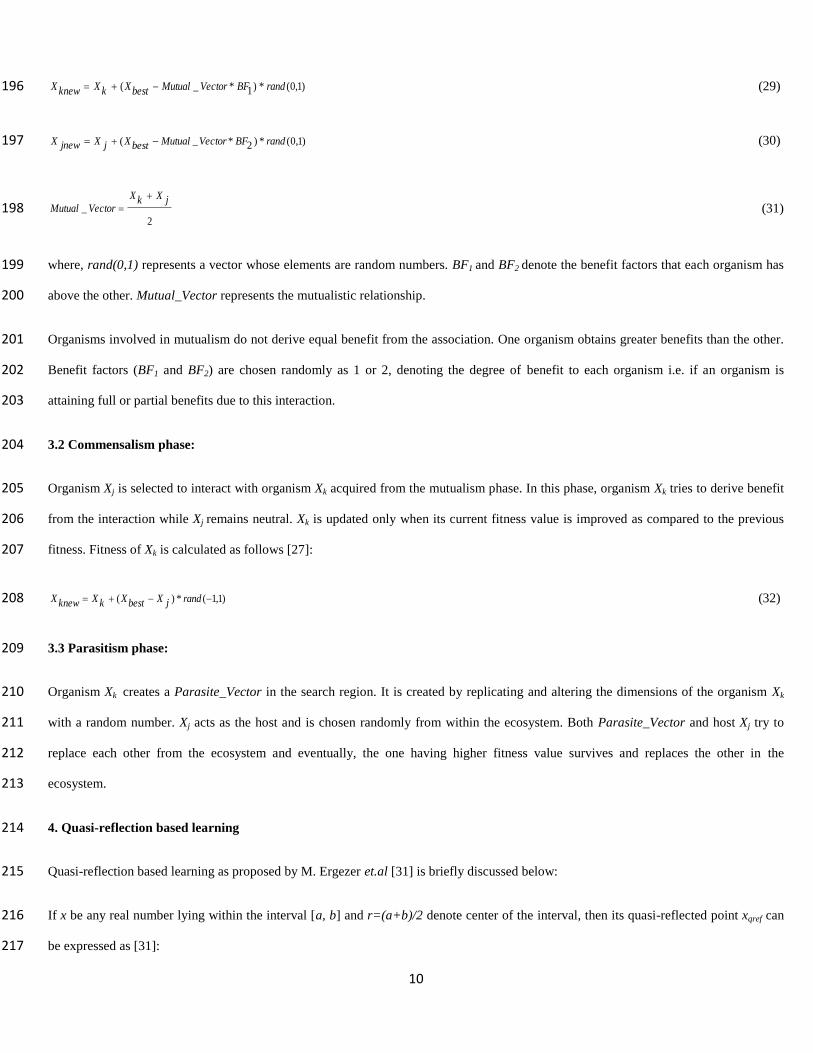
)1,0(*)1*_( randBFVectorMutualbestXkXknewX (29) 196
)1,0(*)2*_( randBFVectorMutualbestXjXjnewX (30) 197
2
_jXkX
VectorMutual
(31) 198
where, rand(0,1) represents a vector whose elements are random numbers. BF1 and BF2 denote the benefit factors that each organism has 199
above the other. Mutual_Vector represents the mutualistic relationship. 200
Organisms involved in mutualism do not derive equal benefit from the association. One organism obtains greater benefits than the other. 201
Benefit factors (BF1 and BF2) are chosen randomly as 1 or 2, denoting the degree of benefit to each organism i.e. if an organism is 202
attaining full or partial benefits due to this interaction. 203
3.2 Commensalism phase: 204
Organism Xj is selected to interact with organism Xk acquired from the mutualism phase. In this phase, organism Xk tries to derive benefit 205
from the interaction while Xj remains neutral. Xk is updated only when its current fitness value is improved as compared to the previous 206
fitness. Fitness of Xk is calculated as follows [27]: 207
)1,1(*)( randjXbestXkXknewX
(32) 208
3.3 Parasitism phase: 209
Organism Xk creates a Parasite_Vector in the search region. It is created by replicating and altering the dimensions of the organism Xk 210
with a random number. Xj acts as the host and is chosen randomly from within the ecosystem. Both Parasite_Vector and host Xj try to 211
replace each other from the ecosystem and eventually, the one having higher fitness value survives and replaces the other in the 212
ecosystem. 213
4. Quasi-reflection based learning 214
Quasi-reflection based learning as proposed by M. Ergezer et.al [31] is briefly discussed below: 215
If x be any real number lying within the interval [a, b] and r=(a+b)/2 denote center of the interval, then its quasi-reflected point xqref can 216
be expressed as [31]: 217
11
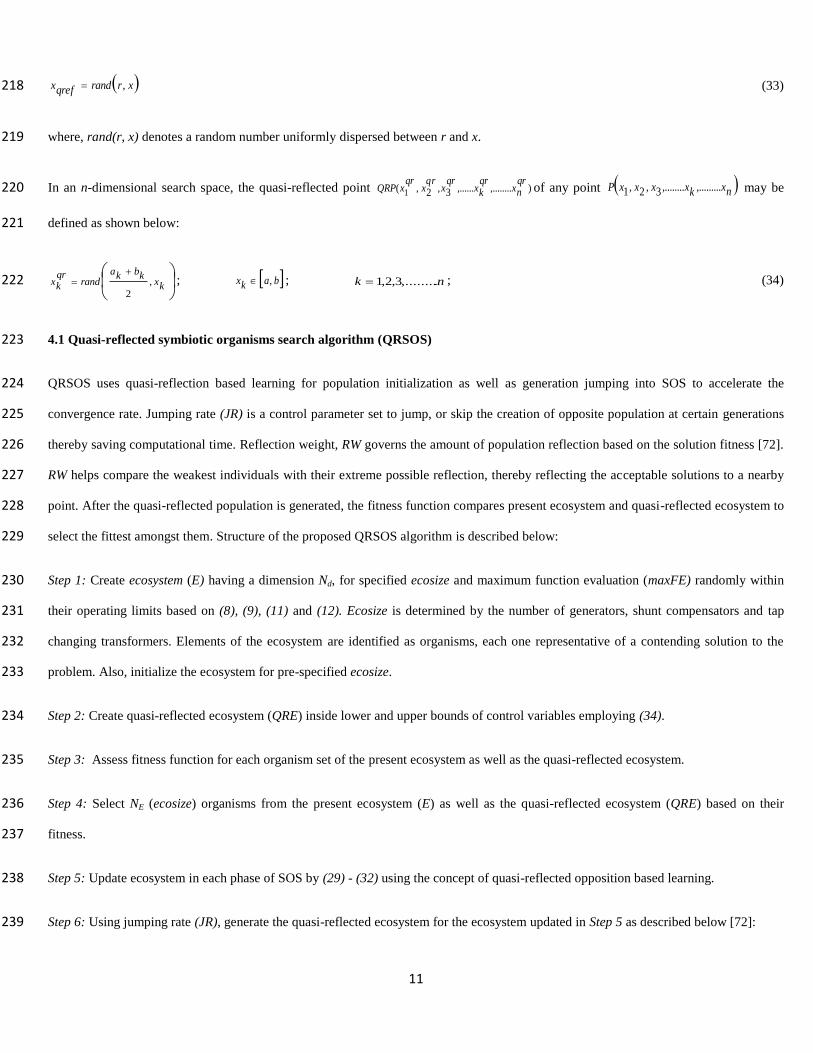
xrrandqrefx , (33) 218
where, rand(r, x) denotes a random number uniformly dispersed between r and x. 219
In an n-dimensional search space, the quasi-reflected point ),........,......3,2,( 1
qrnx
qrkx
qrx
rqx
qrxQRP of any point nxkxxxxP ,.........,........3,2,1 may be 220
defined as shown below: 221
kx
kbkarand
qrkx ,
2
; bakx , ; nk .,.........3,2,1 ; (34) 222
4.1 Quasi-reflected symbiotic organisms search algorithm (QRSOS) 223
QRSOS uses quasi-reflection based learning for population initialization as well as generation jumping into SOS to accelerate the 224
convergence rate. Jumping rate (JR) is a control parameter set to jump, or skip the creation of opposite population at certain generations 225
thereby saving computational time. Reflection weight, RW governs the amount of population reflection based on the solution fitness [72]. 226
RW helps compare the weakest individuals with their extreme possible reflection, thereby reflecting the acceptable solutions to a nearby 227
point. After the quasi-reflected population is generated, the fitness function compares present ecosystem and quasi-reflected ecosystem to 228
select the fittest amongst them. Structure of the proposed QRSOS algorithm is described below: 229
Step 1: Create ecosystem (E) having a dimension Nd, for specified ecosize and maximum function evaluation (maxFE) randomly within 230
their operating limits based on (8), (9), (11) and (12). Ecosize is determined by the number of generators, shunt compensators and tap 231
changing transformers. Elements of the ecosystem are identified as organisms, each one representative of a contending solution to the 232
problem. Also, initialize the ecosystem for pre-specified ecosize. 233
Step 2: Create quasi-reflected ecosystem (QRE) inside lower and upper bounds of control variables employing (34). 234
Step 3: Assess fitness function for each organism set of the present ecosystem as well as the quasi-reflected ecosystem. 235
Step 4: Select NE (ecosize) organisms from the present ecosystem (E) as well as the quasi-reflected ecosystem (QRE) based on their 236
fitness. 237
Step 5: Update ecosystem in each phase of SOS by (29) - (32) using the concept of quasi-reflected opposition based learning. 238
Step 6: Using jumping rate (JR), generate the quasi-reflected ecosystem for the ecosystem updated in Step 5 as described below [72]: 239

12
if rand < JR 240
// Find the absolute of minimum, maximum, and median for the total ecosystem in current generation. 241
// Create reflection weight RW in the interval [0, 1], which determines the amount of reflection based on the fitness of 242
an individual. 243
244
for p = 1 : NE 245
for q = 1 : Nd 246
if Ep,q<Median 247
RWqpEqbqa
qpEqpQRE
,
2,,
248
else 249
RWqbqa
qpEqbqa
qpQRE
2,
2,
250
end 251
end 252
end 253
end 254
255
Step 7: Evaluate the fitness function of the modified E and its QRE. 256
Step 8: Select NE number of fittest organisms from E and QRE. 257
Step 9: Obtain best fitness and best organism. Best fitness denotes minimum of the fitness function assessed for each solution set and best 258
organism denotes the solution set for which best fitness is obtained. 259
Step 10: Go to step 5 and repeat till predefined maxFE. Store best fitness value in an array, identified as the Pareto-optimal set and store 260
best organism in another array. 261
Step 11: For multi-objective formulations from (23) – (28), vary the value of the weighting factor w1 from 0 to 1 in steps of 0.1, and 262
repeat step 1 to step 10 till the value of w1 reaches 1. 263
13
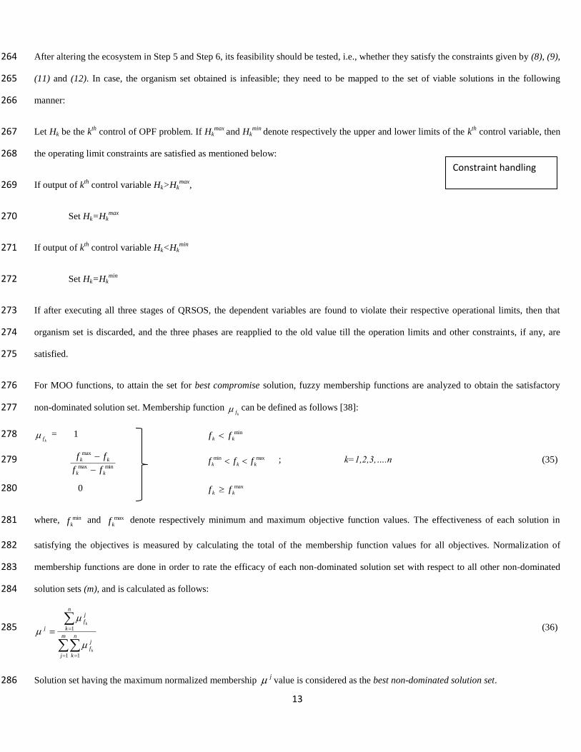
After altering the ecosystem in Step 5 and Step 6, its feasibility should be tested, i.e., whether they satisfy the constraints given by (8), (9), 264
(11) and (12). In case, the organism set obtained is infeasible; they need to be mapped to the set of viable solutions in the following 265
manner: 266
Let Hk be the kth
control of OPF problem. If Hkmax
and Hkmin
denote respectively the upper and lower limits of the kth
control variable, then 267
the operating limit constraints are satisfied as mentioned below: 268
If output of kth
control variable Hk>Hkmax
, 269
Set Hk=Hkmax
270
If output of kth
control variable Hk<Hkmin
271
Set Hk=Hkmin
272
If after executing all three stages of QRSOS, the dependent variables are found to violate their respective operational limits, then that 273
organism set is discarded, and the three phases are reapplied to the old value till the operation limits and other constraints, if any, are 274
satisfied. 275
For MOO functions, to attain the set for best compromise solution, fuzzy membership functions are analyzed to obtain the satisfactory 276
non-dominated solution set. Membership function kf
can be defined as follows [38]: 277
kf = 1 min
kk ff 278
minmax
max
kk
kk
ff
ff
maxmin
kkk fff ; k=1,2,3,….n (35) 279
0 max
kk ff 280
where, min
kf and max
kf denote respectively minimum and maximum objective function values. The effectiveness of each solution in 281
satisfying the objectives is measured by calculating the total of the membership function values for all objectives. Normalization of 282
membership functions are done in order to rate the efficacy of each non-dominated solution set with respect to all other non-dominated 283
solution sets (m), and is calculated as follows: 284
m
j
n
k
j
f
n
k
j
f
j
k
k
1 1
1
(36) 285
Solution set having the maximum normalized membership j value is considered as the best non-dominated solution set. 286
Constraint handling
14
5. Results and Discussion: 287
The algorithm is coded using MATLAB R2014a, and executed in a PC having Intel Core i7 processor clocked at 3.4 GHz, having 2GB 288
RAM. An ecosize of 30 is chosen to simulate the OPF program using QRSOS algorithm. Plots of fitness values of different objective 289
functions are obtained over a span of 100 iterations in each case, to analyse the convergence characteristics of QRSOS. 290
5.1 Description of the test system 291
IEEE 30 bus test system: 292
Data and constraints for this system are obtained from [33]-[36]. Two sets of generator data and the corresponding prohibited zones 293
(Table 1 and Table 6 of Ref. [28]) have been used for analyzing the test cases. 294
5.2 Analysis of the results obtained using QRSOS: 295
Results achieved using QRSOS are analyzed in detail in this sub-section. Bold fonts are used to represent the objective function values 296
and the CPU time for computation. 297
5.2.1 Single objective optimization for IEEE 30 bus test system. 298
Test case 1: OPF problem neglecting effect of VE and POZ. 299
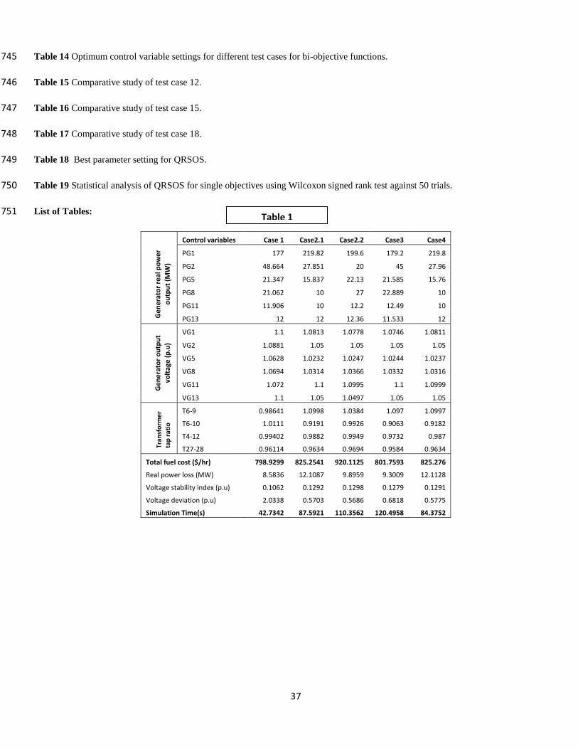
Test case 1 considers the minimization of QFC described by (16) as its objective. Simulation results are demonstrated in Table 1. The 300
optimized fuel cost using QRSOS is attained as 798.9299 $/hr. Comparative study of test case 1 as shown in Table 2 reveal that QFC 301
obtained using the proposed technique is lesser than the best value of 801.5733 $/hr, as obtained using SOS [28]. Also, the result obtained 302
using the proposed algorithm is better when compared to results obtained using other recently applied algorithms like backtracking search 303
algorithm (BSA), artificial bee colony (ABC) optimization, modified shuffle frog leaping algorithm (MSFLA) etc., and others, available 304
in the literature as listed in Table 2. Fig. 2 portrays the convergence characteristic of test case 1. The algorithm converged in less than 305
twenty iterations showing faster convergence than its predecessor. 306
Test case 2: OPF problem considering VE. 307
Test case 2.1: 308
The result obtained for test case 2.1 is provided in Table 1 which is derived employing the generator cost coefficients as given in Table 1 309
in Ref. [28]. The cost function for this objective is formulated using (17). It is seen that FC obtained considering VE using QRSOS 310
algorithm is 825.2541 $/hr. Comparative study for this test case is provided in Table 3. QRSOS provides better result than the previously 311
obtained best value of 825.2985 $/hr, as achieved by SOS in [28]. Fig. 3 depicts the convergence characteristics for this test case and it is 312
found to converge in less than thirty iterations. 313
15
Test case 2.2: Results for this test case are given in Table 1. FC attained considering valve effect using QRSOS algorithm and employing 314
the generator cost coefficients as provided in Table 6 of Ref. [28] is 920.1125 $/hr. The cost function is described by (17). Comparative 315
study is provided in Table 4, which substantiates that the proposed algorithm achieves better result than others to which it is compared. 316
Fig. 4 depicts the convergence characteristics for this case and it is found to converge in about thirty iterations which is less than one-317
sixth of that required by SOS [28]. 318
Test case 3: OPF considering POZ. 319
Generator cost coefficients as provided in Table 1 of Ref. [28] and QFC of (16) is considered. Result obtained for this test case is 320
provided in Table 4. Table 5 provides a comparative study of this test case. QRSOS reduces objective function value to 801.7593 $/hr 321
from the previously obtained best value of 801.8398 $/hr in [28]. Fig. 5 depicts the convergence characteristics for this method showing 322
faster convergence in less than 45 iterations, which is nearly 36.36 % of that required by SOS in [28]. 323
Test case 4: OPF problem considering both VE and POZ. 324
Generator cost coefficients provided in Table 1 of [28] and cost function as described by (17) is considered. The result for this case is 325
tabulated in Table 1. Comparative study for this objective is presented in Table 6 demonstrating competitiveness of the proposed 326
algorithm in achieving a lower cost. Fig. 6 shows a faster convergence curve for this test case when compared to SOS [28]. 327
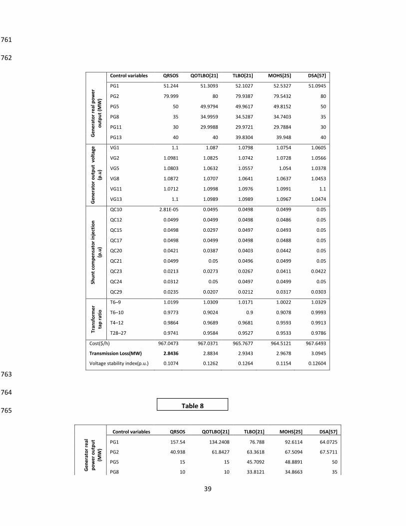
Test case 5: OPF problem with the objective of RTL minimization 328
Objective for this test case is formulated using (19). Table 7 lists the optimal control variables for this objective. 329
The suggested algorithm is capable to bring down loss to 2.8423 MW, which is lower than that obtained using QOTLBO, TLBO, MOHS 330
and DSA in literature. Also the result obtained using QRSOS is 1.42% lower than the previous best result of 2.8834 MW [21]. For this 331
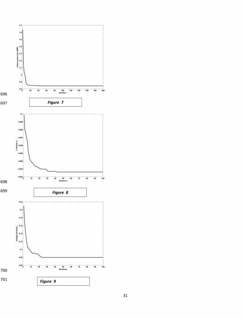
case, QRSOS took less than 35 iterations to convergence which is lower than that observed in [21] as depicted in Fig. 7. 332
Test case 6: OPF for L-index minimization 333
This case considers lowering L-index value for improving voltage stability of the system using (20). Control parameters for this case are 334
listed in Table 8 below: 335
It can be observed that the proposed methodology lowers the value of this objective function to 0.092613 p.u, which is lowest as 336
compared to those obtained using QOTLBO, TLBO, MOHS and DSA. Also it lowered the L-index value by 6.82% from the previous 337
best-reported value of 0.0994 p.u [21]. Fig. 8 shows a quicker rate of convergence for this case too. 338
16
Test case 7: Voltage deviation (VD) minimization 339
This test case considers improving the load voltage profile of the system using (21). Optimal control parameters attained for this case are 340
listed in Table 9: 341
QRSOS lowered the VD value to 0.079866 p.u, by a high margin of 78.98% compared to NSGA-II in [23]. The transmission loss is also 342
reduced to a great extent. The algorithm converged within 25 iterations for this test case as observed in Fig 9. 343
5.2.2 Single objective optimization for IEEE 118 bus test system. 344
To check the competence of the offered algorithm in a large system, IEEE 118 bus test system is taken into consideration for studying 345
different test cases. Data for the system is obtained from Ref. [58]. Penalty factors have been assigned to the objectives as per (14) to 346
handle the possible constraint violations for this large system. The penalty factors are considered in the range of [10000 100000] and 347
tuning has been done in steps of 10000. Results for all penalty factors are not shown here for page limitations. Optimum results have been 348
obtained for a penalty factor of 30000 assigned to the objectives which are tabulated in subsequent test cases: 349
Test case 8: OPF problem for QFC minimization. 350
Optimal results are obtained for a penalty factor of 30000 assigned to the objective. The results and their comparisons are provided in 351
Table 10. 352
As can be observed from the above table, QRSOS effectively reduced the fuel cost by a large margin of 14.30% from 55,968.14 $/hr [21] 353
to 47,960 $/hr. Also, it effectively reduced the emission from 410.9816 lb/hr [21] to a much lower value of 342.635 lb/hr in case of single 354
objective optimization itself. It achieved better result than those of QOTLBO and TLBO in [21]. The proposed algorithm showed rapid 355
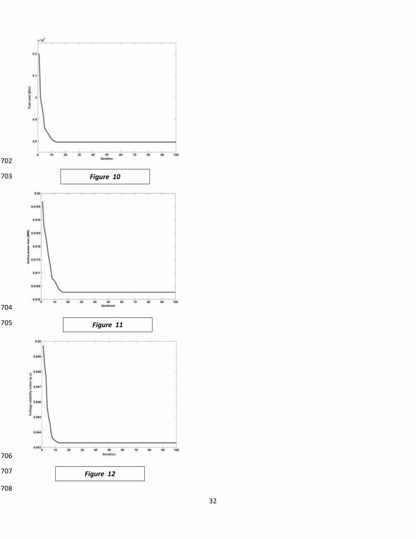
convergence in fewer than 20 iterations as seen in Fig. 10. 356
Test case 9: OPF problem for real power transmission loss minimization. 357
This test case considered minimizing the real power loss that occurs during transmission using (18). A penalty factor of 30000 assigned to 358
the loss minimization objective gave optimum results which are listed in Table 11. 359
*The unit of the result obtained using QOTLBO for loss minimization in [21] is given as KW, whereas, the real value comes as 35.3191 MW after calculation using 360 the parameters provided by the authors. 361
362
17
QRSOS is proficient in reducing the transmission loss to 16.27 MW, nearly half of that of 35.3191 MW and 36.8482 MW obtained 363
respectively by QOTLBO and TLBO as reported in [21]. Simultaneously it is also able to reduce the emission by 6.5127 lb/hr compared 364
to that obtained by QOTLBO. Fig.11 shows rapid convergence in less than 20 iterations. 365
Test case 10: OPF problem for minimizing L-index. 366
L-index of large IEEE 118 bus has been considered for improvement of voltage profile using (19). As it is very difficult to maintain the 367
voltage stability in case of a large system, a penalty factor of 30000 has been assigned to the objective to handle inequality constraints. 368
Optimum control parameters obtained for this test case are listed in Table 12: 369
Optimal value of VSI is obtained as 0.0433 p.u, which denotes a stable system. Fig. 12 shows the convergence characteristic of test case 370
10. Convergence is achieved in fewer than 15 iterations. 371
Test case 11: OPF problem for emission minimization objective 372
This test case considers minimizing emission of pollutants to the atmosphere. The objective is formulated using (21). A penalty factor of 373
30000 assigned to the objective provided optimal results while effectively handling the constraints. Optimal parameters of this test case 374
are listed in Table 13: 375
QRSOS provided lowest emission value when compared to those obtained using QOTLBO and TLBO. It effectively reduced the 376
emission from 176.1666 lb/hr in [21] to 164.5 lb/hr, i.e., by a margin of 6.62%. Also it reduced the fuel cost by 3.29% from 65,601.64 377
$/hr [21] and transmission loss by 7.58% from the previously reported best value of 150.9366 MW [21] simultaneously. Fig. 13 shows 378
the convergence for this case. 379
5.2.3 Bi-objective results for IEEE 30 bus test system 380
Nine different case studies have been done on the IEEE 30 bus test system for diverse MOO functions and their pareto-fronts have been 381
studied. 382
A Pareto optimal solution is defined as the finest solution set selected from numerous solution sets in which all objectives are equally 383
compromised with respect to one another. Each solution set is defined as non-dominated solution set. There can be an infinite number of 384
Pareto solution sets for a multi-objective optimization problem. 385
Test case 12: OPF problem for simultaneously minimizing QFC and RTL. 386

18
This objective function is described using (23) and results are presented in Table 14. Comparative study depicted in Table 15 shows that 387
the algorithm achieved better result compared to those obtained using MO-DEA, QOTLBO, TLBO, MOHS and NSGA-II in literature. 388
Compared to MO-DEA, QRSOS lowered the transmission loss from 5.5949 MW [64] by 1.69 % to 5.5002 MW. But at the same time, 389
the total FC increased by a small margin of 0.071 %. It is observed that VSI value has improved simultaneously thereby increasing the 390
voltage stability margin. Fig. 14 depicts the Pareto-front obtained for the above objective. 391
Test case 13: OPF for simultaneously minimizing FC and RTL considering VE. 392
Generator cost coefficients provided in Table 1 of [28] are used for this objective described using (24). Results are presented in Table 14. 393
Total FC attained using QRSOS is 833.3756 $/hr which is 0.98% higher when compared to case 2.1 and the RTL is 9.7887 MW which is 394
19.16% lower than that of case 2.1. Fig. 15 represents the Pareto front obtained for test case 13. No existing results available in the 395
literature for doing comparative study. 396
Test case 14: OPF for minimizing FC along with RTL considering both VE and POZ. 397
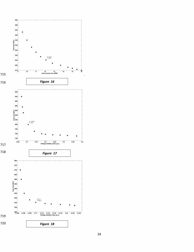
Generator cost coefficients and the POZs as provided in Table 1 of Ref. [28] are used in (24). From Table 14, it can be witnessed that 398
total FC is 825.2938 $/hr and the RTL is 12.0904 MW. The total FC was increased by a slight margin of 0.002% and RTL was reduced 399
by 0.18% when compared to single objective minimization of case 4. Fig. 16 represents the Pareto-front for this test case. No existing 400
results available in the literature for doing comparative study. 401
Test case 15: OPF for simultaneously minimizing QFC and L-index neglecting VE and POZ. 402
This objective function is described using (25). Table 14 demonstrates result obtained for this bi-objective function. Table 16 403
demonstrates that QRSOS reduced the total QFC to 799.0175 $/hr, which is lower than those obtained using QOTLBO, TLBO, NSGA-II, 404
MOHS and recently applied BSA and MO-DEA in literature. Comparing the result with those of latest algorithms like BSA [63] and MO-405
DEA [64], it is seen that QRSOS lowers the QFC value by 0.0803%. Simultaneously, it could lower the VSI value to 0.1067 p.u by 406
15.25% from the latest MO-DEA [64] thereby ensuring a stable system. Fig. 17 represents the Pareto front for this bi-objective function. 407
Test case 16: OPF for simultaneously minimizing FC and VSI considering VE. 408
Generator cost coefficients as provided in Table 1 of [28] are used for this case described by (26). Results attained for this test case are 409
tabulated in Table 14. Fig. 18 shows the Pareto-front for this objective function. Overall FC for this bi-objective function came out to be 410
835.2938 $/hr and the VSI as 0.1072 p.u. The FC increased by a negligible margin of 1.21% and the VSI reduced by 17.70% when 411
compared to single objective minimization of case 2.1. No existing results available in literature for comparison. 412
19
Test case 17: OPF for simultaneously minimizing FC and VSI considering VE and POZ. 413
Generator cost coefficients and POZs as provided in Table 1 of [28] is used for test case described by (26).Result obtained for this test 414
case is demonstrated in Table 14. QRSOS achieved FC of 825.4182 $/hr and VSI of 0.1277 p.u. The total FC increased by a negligible 415
margin of 0.017% whereas the VSI improved by a margin of 1.08% when compared to single objective minimization of case 4. Fig. 19 416
represents the Pareto-front for this case. No existing results available in the literature for comparison. 417
Test case 18: OPF for minimizing QFC along with VD 418
This objective function is defined using (27). Results obtained for this test case are demonstrated in Table 14. VD obtained using QRSOS 419
is 0.0991 p.u which is 94.09% lower, and the total FC is 803.3138 $/hr which is 0.55% higher when compared to single objective 420
minimization of case 1. Also, when compared to the recently applied techniques, such as BSA [63] and MO-DEA [64], it is observed 421
from Table 17, that QRSOS lowers the FC as well as VD by 0.074 % and 14.42 % respectively. Fig. 20 depicts the Pareto front for this 422
test case. 423
Test case 19: OPF to minimize FC along with VD considering VE. 424
Generator cost coefficients from Table 1 of [28] is used for the case described using (28). Result obtained for this test case is 425
demonstrated in Table 14. The total FC achieved using QRSOS is 842.5288 $/hr which is 2.05 % higher than that in test case 2.1 and VD 426
is achieved as 0.0832 p.u which is 85.41% less than that obtained for single objective minimization of case 2.1. Fig. 21 represents the 427
Pareto-front for this case. No existing results available in the literature for comparison. 428
Test case 20: OPF for minimizing FC along with VD considering VE and POZ. 429
Generator cost coefficients and POZs in Table 1 of [28] are used for the case described using (28).Results are presented in Table 14. The 430
total FC achieved using QRSOS is 832.7439 $/hr which is 0.904% higher and VD is achieved as 0.1461 p.u, which is 74.70% lower when 431
compared to the single objective minimization of case 4. Fig. 22 represents the Pareto-front for this case. No existing results are available 432
in the literature for carrying out a comparative study for this case too. 433
Analyses of the aforementioned case studies prove supremacy of the proposed technique over other algorithms such as QOTLBO, TLBO, 434
MOHS, NSGA-II, ABC, BSA, PSO, DE-PSO, EP, IEP, GA, IABC, SA, SFLA, MSFLA, NLP, TS, ACO, Hybrid SFLA-SA, and SOS 435
available in literature in achieving optimum solution for the OPF problem. QRSOS produces superior solutions in comparison to other 436
algorithms mentioned above for the cases studied. Pareto fronts obtained for each of the multi-objective functions depict solution sets 437
well distributed in the search space signifying non-dominated solution. 438

20
Determination of best parameter settings for QRSOS 439
To determine the best parameter setting for QRSOS to deliver efficient results, population sizes of 10, 20, 30, 40 and 50 have been taken 440
into consideration. For each population size, jumping rate JR is augmented from 0.1 to 0.9 in steps of 0.1 as shown in Table 18. 441
Performance of QRSOS in test case 4 is analyzed considering all the aforementioned combinations. 50 different trials have been carried 442
out with 100 iterations for each trial. From Table 18, it is observed that a population size of 30 and a jumping rate (JR) of 0.3 gives the 443
best fuel cost value of 825.2760 $/hr, which is less than previous best reported value of 825.3705 $/hr. 444
Statistical analysis of test results 445
Statistical analysis is done on 50 trial data sets to assess the performance of QRSOS. For this purpose, one trial data set, as obtained from 446
the solution sets of the proposed algorithm, is tested using Wilcoxon signed rank test (WSRT). A p-value (probability value) below 0.05 447
obtained from this test reflects as ample proof to counter the null hypothesis. p-values obtained using this test for cases 1-4, along with 448
minimum, maximum, average values and standard deviation are tabulated below: 449
As observed from the above Table 19, p-value in every case is well below the desired value of 0.05 establishing statistical significance of 450
the results. Also, the standard deviation values obtained for QRSOS are much lower than those obtained by its predecessor [28] for all the 451
cases. 452
6. Conclusion 453
The aim of this paper was to introduce a novel technique designated as quasi-reflected symbiotic organisms search algorithm (QRSOS) to 454
solve the OPF problem. The technique has been successfully applied to the OPF problem to solve both single objective and bi- objective 455
functions. Twenty different test cases were solved with and without considering the VE and POZs. Outputs obtained using QRSOS have 456
been compared with those obtained by SOS, QOTLBO, TLBO, MOHS, NSGA-II, DE, PSO and several other techniques as reported in 457
the literature. Results obtained demonstrate the efficiency and robustness of the offered technique in handling OPF problem for both 458
small and large-scale test systems. Results have shown marked improvement for QRSOS when compared to other available techniques. It 459
has passed the Wilcoxon signed rank test with very low p-values and established its statistical significance. It has been simultaneously 460
observed that this algorithm acquired very fast convergence in all cases when matched to other techniques. Henceforth, it may be deduced 461
that QRSOS algorithm is promising and there is a possibility for future research in this direction considering other aspects of power 462
system. 463
464
21
Future scope 465
The proposed technique has effectively handled both linear and non-linear objectives. Since QRSOS was able to solve the OPF problem 466
successfully, it may be further applied to solve OPF, considering renewables and uncertainty due to load demands under different 467
contingency scenarios. 468
Acknowledgement 469
The authors would like to acknowledge the lab facilities provided by the Electrical Engineering Department for carrying out the research 470
work. 471
Declaration of conflict of interest 472
The authors hereby declare that there is no conflict of interest for the work presented in this paper. 473
Declaration of submission 474
The authors hereby declare that the article has neither been published nor is in consideration for publication elsewhere in any form. Also, 475
if accepted for publication, the manuscript will not be published elsewhere in any form without the written consent of the copyright 476
holder. 477
References: 478
1. De Carvalho, E.P., dos Santos, A. and Ma, T.F. "Reduced gradient method combined with augmented Lagrangian and barrier for 479
the optimal power flow problem", Applied Mathematics and Computation, 200(2), pp.529-536 (2008). 480
2. Momoh, J.A., Adapa, R. and El-Hawary, M.E. “A review of selected optimal power flow literature to 1993. I. Nonlinear and 481
quadratic programming approaches”, IEEE transactions on power systems, 14(1), pp.96-104 (1999). 482
3. Santos, A.J. and Da Costa, G.R.M. “Optimal-power-flow solution by Newton's method applied to an augmented Lagrangian 483
function”, IEE Proceedings-Generation, Transmission and Distribution, 142(1), pp.33-36 (1995). 484
4. Yan, X. and Quintana, V.H. “Improving an interior-point-based OPF by dynamic adjustments of step sizes and tolerances”, 485
IEEE Transactions on Power Systems, 14(2), pp.709-717 (1999). 486
5. Huneault, M. and Galiana, F.D. “A survey of the optimal power flow literature”, IEEE transactions on Power Systems, 6(2), 487
pp.762-770 (1991). 488
22
6. Zhang, S. and Irving, M.R. “Enhanced Newton-Raphson algorithm for normal, controlled and optimal power flow solutions 489
using column exchange techniques”, IEE Proceedings-Generation, Transmission and Distribution, 141(6), pp.647-657 (1994). 490
7. Habibollahzadeh, H., Luo, G.X. and Semlyen, A. “Hydrothermal optimal power flow based on a combined linear and nonlinear 491
programming methodology”, IEEE Transactions on Power Systems, 4(2), pp.530-537 (1989). 492
8. Burchett, R.C., Happ, H.H. and Vierath, D.R. “Quadratically convergent optimal power flow”, IEEE Transactions on Power 493
Apparatus and Systems, (11), pp.3267-3275 (1984). 494
9. Yuryevich, J. and Wong, K.P. “Evolutionary programming based optimal power flow algorithm”, IEEE transactions on Power 495
Systems, 14(4), pp.1245-1250 (1999). 496
10. Lai, L.L., Ma, J.T., Yokoyama, R. and Zhao, M. “Improved genetic algorithms for optimal power flow under both normal and 497
contingent operation states”, International Journal of Electrical Power & Energy Systems, 19(5), pp.287-292 (1997). 498
11. Swain, A.K. and Morris, A.S. “A novel hybrid evolutionary programming method for function optimization”, In Evolutionary 499
Computation, 2000, Proceedings of the 2000 Congress on (Vol. 1, pp. 699-705). IEEE (2000). 500
12. Abido, M.A. “Optimal power flow using particle swarm optimization”, International Journal of Electrical Power & Energy 501
Systems, 24(7), pp.563-571 (2002). 502
13. El Ela, A.A., Abido, M.A. and Spea, S.R. “Optimal power flow using differential evolution algorithm”, Electric Power Systems 503
Research, 80(7), pp.878-885 (2010). 504
14. Abido, M.A. “Optimal power flow using tabu search algorithm”, Electric Power Components and Systems, 30(5), pp.469-483 505
(2002). 506
15. Cai, J., Ma, X., Li, L., Yang, Y., Peng, H. and Wang, X. “Chaotic ant swarm optimization to economic dispatch”, Electric Power 507
Systems Research, 77(10), pp.1373-1380 (2007). 508
16. Roy, P.K., Ghoshal, S.P. and Thakur, S.S. “Biogeography based optimization for multi-constraint optimal power flow with 509
emission and non-smooth cost function”, Expert Systems with Applications, 37(12), pp.8221-8228 (2010). 510
17. Tripathy, M. and Mishra, S. “Bacteria foraging-based solution to optimize both real power loss and voltage stability limit”, IEEE 511
Transactions on power systems, 22(1), pp.240-248 (2007). 512
18. Khazali, A.H. and Kalantar, M. “Optimal reactive power dispatch based on harmony search algorithm”, International Journal of 513
Electrical Power & Energy Systems, 33(3), pp.684-692 (2011). 514
19. Roy, P.K., Mandal, B. and Bhattacharya, K. “Gravitational search algorithm based optimal reactive power dispatch for voltage 515
stability enhancement”, Electric Power Components and Systems, 40(9), pp.956-976 (2012). 516
20. Basu, M. “Teaching–learning-based optimization algorithm for multi-area economic dispatch”, Energy, 68, pp.21-28 (2014). 517

23
21. Mandal, B. and Roy, P.K. “Multi-objective optimal power flow using quasi-oppositional teaching learning based optimization”, 518
Applied Soft Computing, 21, pp.590-606 (2014). 519
22. Abido, M.A. “Multiobjective particle swarm optimization for optimal power flow problem”, In Handbook of swarm intelligence, 520
(pp. 241-268) (2011). Springer Berlin Heidelberg. 521
23. Hernandez, Y.R. and Hiyama, T. “Minimization of voltage deviations, power losses and control actions in a transmission power 522
system”, In Intelligent System Applications to Power Systems, 2009. ISAP'09. 15th International Conference on (pp. 1-5). IEEE 523
(November 2009). 524
24. Roy, P.K., Ghoshal, S.P. and Thakur, S.S. “Multi-objective optimal power flow using biogeography-based optimization”, 525
Electric Power Components and Systems, 38(12), pp.1406-1426 (2010). 526
25. Sivasubramani, S. and Swarup, K.S. “Multi-objective harmony search algorithm for optimal power flow problem”, International 527
Journal of Electrical Power & Energy Systems, 33(3), pp.745-752 (2011). 528
26. Bhattacharya, A. and Chattopadhyay, P.K. “Application of biogeography-based optimisation to solve different optimal power 529
flow problems”, IET generation, transmission & distribution, 5(1), pp.70-80 (2011). 530
27. Cheng, M.Y. and Prayogo, D. “Symbiotic organisms search: a new metaheuristic optimization algorithm”, Computers & 531
Structures, 139, pp.98-112 (2014). 532
28. Duman, S. “Symbiotic organisms search algorithm for optimal power flow problem based on valve-point effect and prohibited 533
zones”, Neural Computing and Applications, pp.1-15 (2016). 534
29. Tizhoosh, H.R. “Opposition-based learning: a new scheme for machine intelligence”, In Computational intelligence for 535
modelling, control and automation, 2005 and international conference on intelligent agents, web technologies and internet 536
commerce, international conference on (Vol. 1, pp. 695-701). IEEE (November, 2005). 537
30. Rahnamayan, S., Tizhoosh, H.R. and Salama, M.M. “Quasi-oppositional differential evolution”, In Evolutionary Computation, 538
2007. CEC 2007. IEEE Congress on (pp. 2229-2236). IEEE (September, 2007). 539
31. Ergezer, M., Simon, D. and Du, D. “Oppositional biogeography-based optimization”, In Systems, Man and Cybernetics, 2009. 540
SMC 2009. IEEE International Conference on (pp. 1009-1014). IEEE (October, 2009). 541
32. Zhang, C., Ni, Z., Wu, Z. and Gu, L. “A novel swarm model with quasi-oppositional particle”, In Information Technology and 542
Applications, 2009. IFITA'09. International Forum on (Vol. 1, pp. 325-330). IEEE (May, 2009). 543
33. Alsac, O. and Stott, B. “Optimal load flow with steady-state security”, IEEE transactions on power apparatus and systems, (3), 544
pp.745-751 (1974). 545

24
34. Kılıç, U. “Backtracking search algorithm-based optimal power flow with valve point effect and prohibited zones”, Electrical 546
Engineering, 97(2), pp.101-110 (2015). 547
35. Narimani, M.R., Azizipanah-Abarghooee, R., Zoghdar-Moghadam-Shahrekohne, B. and Gholami, K. “A novel approach to 548
multi-objective optimal power flow by a new hybrid optimization algorithm considering generator constraints and multi-fuel 549
type”, Energy, 49, pp.119-136 (2013). 550
36. Bakirtzis, A.G., Biskas, P.N., Zoumas, C.E. and Petridis, V. “Optimal power flow by enhanced genetic algorithm”, IEEE 551
Transactions on power Systems, 17(2), pp.229-236 (2002). 552
37. Saini, A., Chaturvedi, D.K. and Saxena, A.K. “Optimal power flow solution: a GA-fuzzy system approach”, International 553
journal of emerging electric power systems, 5(2), pp.1-21 (2006). 554
38. Niknam, T., rasoul Narimani, M., Jabbari, M. and Malekpour, A.R. “A modified shuffle frog leaping algorithm for multi-555
objective optimal power flow”, Energy, 36(11), pp.6420-6432 (2011). 556
39. Ongsakul, W. and Bhasaputra, P. “Optimal power flow with FACTS devices by hybrid TS/SA approach”, International journal 557
of electrical power & energy systems, 24(10), pp.851-857 (2002). 558
40. Sayah, S. and Zehar, K. “Modified differential evolution algorithm for optimal power flow with non-smooth cost 559
functions”, Energy conversion and Management, 49(11), pp.3036-3042 (2008). 560
41. Ongsakul, W. and Tantimaporn, T. “Optimal power flow by improved evolutionary programming”, Electric Power Components 561
and Systems, 34(1), pp.79-95 (2006). 562
42. Sood, Y.R. “Evolutionary programming based optimal power flow and its validation for deregulated power system 563
analysis”, International Journal of Electrical Power & Energy Systems, 29(1), pp.65-75 (2007). 564
43. Bouktir, T., Slimani, L. and Mahdad, B. “Optimal power dispatch for large scale power system using stochastic search 565
algorithms”, International Journal of Power & Energy Systems, 28(2), p.118 (2008). 566
44. Yuryevich, J. and Wong, K.P. “Evolutionary programming based optimal power flow algorithm”, IEEE transactions on Power 567
Systems, 14(4), pp.1245-1250 (1999). 568
45. Bouktir, T., Labdani, R. and Slimani, L. “Economic power dispatch of power system with pollution control using multiobjective 569
particle swarm optimization”, Journal of Pure & Applied Sciences, 4(2), pp.57-77 (2007). 570
46. Niknam, T., Narimani, M.R., Aghaei, J., Tabatabaei, S. and Nayeripour, M. “Modified honey bee mating optimisation to solve 571
dynamic optimal power flow considering generator constraints”, IET generation, transmission & distribution, 5(10), pp.989-572
1002 (2011). 573
25
47. Abido, M.A. “Optimal power flow using tabu search algorithm”, Electric Power Components and Systems, 30(5), pp.469-483 574
(2002). 575
48. Basu, M. “Multi-objective optimal power flow with FACTS devices”, Energy Conversion and Management, 52(2), pp.903-910 576
(2011). 577
49. Malik, T.N., ul Asar, A., Wyne, M.F. and Akhtar, S. “A new hybrid approach for the solution of nonconvex economic dispatch 578
problem with valve-point effects”, Electric Power Systems Research, 80(9), pp.1128-1136 (2010). 579
50. Thitithamrongchai, C. and Eua-Arporn, B. “Self-adaptive differential evolution based optimal power flow for units with non-580
smooth fuel cost functions”, Journal of Electrical Systems, 3(2), pp.88-99 (2007). 581
51. Özyön, S., Yaşar, C., Özcan, G. and Temurtaş, H. “An artificial bee colony algorithm (abc) aproach to nonconvex economic 582
power dispatch problems with valve point effect”. In National Conference on Electrical, Electronics and Computer (FEEB’11) 583
pp (pp. 294-299), (2011). 584
52. Yaşar, C. and Özyön, S. “A new hybrid approach for nonconvex economic dispatch problem with valve-point 585
effect”, Energy, 36(10), pp.5838-5845 (2011). 586
53. AydıN, D. and Özyön, S. “Solution to non-convex economic dispatch problem with valve point effects by incremental artificial 587
bee colony with local search”, Applied Soft Computing, 13(5), pp.2456-2466 (2013). 588
54. Wilcoxon, F. “Individual comparisons by ranking methods”, Biometrics bulletin, 1(6), pp.80-83 (1945). 589
55. Lee, F.N. and Breipohl, A.M. “Reserve constrained economic dispatch with prohibited operating zones”, IEEE transactions on 590
power systems, 8(1), pp.246-254 (1993). 591
56. https://www.researchgate.net/profile/Hamed_Zeinoddini-592
Meymand/publication/220199759/figure/fig3/AS:277225963311109@1443107228843/Fig-3-Cost-function-of-a-generator-with-593
prohibited-operating-zones.png search optimization algorithm. International Journal of Electrical Power & Energy Systems, 81, 594
64-77. 595
57. Abaci, K. and Yamacli, V. “Differential search algorithm for solving multi-objective optimal power flow 596
problem”, International Journal of Electrical Power & Energy Systems, 79, pp.1-10 (2016). 597
58. The Electrical and Computer Engineering Department, Illinois Institute of Technology, Data, IEEE 118-bus test system data. 598
Available at: http://motor.ece.iit.edu/data/JEAS IEEE118.doc 599
59. Ghasemi, M., Ghavidel, S., Aghaei, J., Gitizadeh, M. and Falah, H. “Application of chaos-based chaotic invasive weed 600
optimization techniques for environmental OPF problems in the power system”, Chaos, Solitons & Fractals, 69, pp.271-284 601
(2014). 602

26
60. Ghasemi, M., Ghavidel, S., Rahmani, S., Roosta, A. and Falah, H. “A novel hybrid algorithm of imperialist competitive 603
algorithm and teaching learning algorithm for optimal power flow problem with non-smooth cost functions”, Engineering 604
Applications of Artificial Intelligence, 29, pp.54-69 (2014). 605
61. Ghasemi, M., Ghavidel, S., Ghanbarian, M.M., Massrur, H.R. and Gharibzadeh, M., 2014. Application of imperialist 606
competitive algorithm with its modified techniques for multi-objective optimal power flow problem: a comparative 607
study. Information Sciences, 281, pp.225-247. 608
62. Ghasemi, M., Ghavidel, S., Ghanbarian, M.M., Gharibzadeh, M. and Vahed, A.A. “Multi-objective optimal power flow 609
considering the cost, emission, voltage deviation and power losses using multi-objective modified imperialist competitive 610
algorithm”, Energy, 78, pp.276-289 (2014). 611
63. Chaib, A.E., Bouchekara, H.R.E.H., Mehasni, R. and Abido, M.A., “Optimal power flow with emission and non-smooth cost 612
functions using backtracking search optimization algorithm”, International Journal of Electrical Power & Energy Systems, 81, 613
pp.64-77 (2016). 614
64. Shaheen, A.M., El-Sehiemy, R.A. and Farrag, S.M. “Solving multi-objective optimal power flow problem via forced initialised 615
differential evolution algorithm”, IET Generation, Transmission & Distribution, 10(7), pp.1634-1647 (2016). 616
65. Reddy, S.S., Bijwe, P.R. and Abhyankar, A.R. “Faster evolutionary algorithm based optimal power flow using incremental 617
variables”, International Journal of Electrical Power & Energy Systems, 54, pp.198-210 (2014). 618
66. Reddy, S.S., Abhyankar, A.R. and Bijwe, P.R. “Reactive power price clearing using multi-objective 619
optimization”, Energy, 36(5), pp.3579-3589 (2011). 620
67. Reddy, S.S. and Rathnam, C.S. “Optimal power flow using glowworm swarm optimization”, International Journal of Electrical 621
Power & Energy Systems, 80, pp.128-139 (2016). 622
68. Reddy, S.S. and Bijwe, P.R. “Day-Ahead and Real Time Optimal Power Flow considering Renewable Energy 623
Resources”, International Journal of Electrical Power & Energy Systems, 82, pp.400-408 (2016). 624
69. Reddy, S.S. “Optimal power flow with renewable energy resources including storage”, Electrical Engineering, pp.1-11 (2016). 625
70. Das, A.K., Majumdar, R., Panigrahi, B.K. and Reddy, S.S. “Optimal power flow for indian 75 bus system using differential 626
evolution”, In International Conference on Swarm, Evolutionary, and Memetic Computing (pp. 110-118) (December, 2011). 627
Springer Berlin Heidelberg. 628
71. Mandal, Barun, and Provas Kumar Roy. "Optimal reactive power dispatch using quasi-oppositional teaching learning based 629
optimization." International Journal of Electrical Power & Energy Systems,53, pp. 123-134 (2013). 630
27
72. Bhattacharya, Aniruddha, and P. K. Chattopadhyay. "Solution of economic power dispatch problems using oppositional 631
biogeography-based optimization." Electric Power Components and Systems 38, no. 10 , pp. 1139-1160 (2010). 632
633
634
Anulekha Saha received her B.Tech degree in Electrical Engg. from Birbhum Institute of Engineering and Technology, 635
India, and M.Tech from the department of Electrical Engg., NIT Agartala in 2010 and 2012 respectively. Presently, she 636
is a research scholar in the department of electrical engineering, NIT Agartala. Her research area deals with power 637
system optimization using various soft-computing techniques. 638
Dr. A.K. Chakraborty received his L.L.E from the State Council of Engg. and Technical Education, West Bengal in 639
1979, B.E.E from Jadavpur University in 1987, M.Tech (Power System) from IIT Kharagpur in 1990 and Ph.D (Engg) in 640
2007 from Jadavpur University respectively. He has sixteen years of teaching and fourteen years of industrial 641
experiences. His areas of interest include Application of soft computing techniques to different power system problems, 642
Power Quality, FACTS & HVDC and Deregulated Power System. He worked as a Professor with the college of 643
Engineering & Management, Kolaghat and is presently working as an Associate Professor in the Department of 644
Electrical Engineering, NIT Agartala, India. 645
Dr. Priyanath Das obtained his B.Tech and M.Tech in Electrical Engineering in 1994 and 2002 respectively. He 646
completed his PhD from Jadavpur University in 2013. He is presently working as an Associate Professor in the 647
Department of Electrical Engineering, NIT Agartala, India. He has published several papers in national and international 648
conferences and journals. His areas of interest include Application of FACTS & HVDC, Deregulated Power System and 649
High Voltage Engineering. 650
List of figure captions: 651
Fig. 1 Representation of fuel cost with prohibited operating zones [56]. 652
Fig. 2 Convergence characteristic of test case 1. 653
Fig. 3 Convergence characteristic of test case 2.1. 654
Fig. 4 Convergence characteristic of test case 2.2. 655
Fig. 5 Convergence characteristic of test case 3. 656
Fig. 6 Convergence characteristic of test case 4. 657
Fig. 7 Convergence characteristic of test case 5. 658
28
Fig. 8 Convergence characteristic of test case 6. 659
Fig. 9 Convergence characteristic of test case 7. 660
Fig. 10 Convergence characteristic of test case 8 obtained using QRSOS. 661
Fig. 11 Convergence characteristic of test case 9. 662
Fig. 12 Convergence characteristic of test case 10. 663
Fig. 13 Convergence characteristic of test case 11. 664
Fig. 14 Pareto front for test case 12. 665
Fig. 15 Pareto front for test case 13. 666
Fig. 16 Pareto front for test case 14. 667
Fig. 17 Pareto front for test case 15. 668
Fig. 18 Pareto front for test case 16. 669
Fig. 19 Pareto front for test case 17 obtained using QRSOS. 670
Fig. 20: Pareto front for test case 18. 671
Fig. 21 Pareto front for test case 19. 672
Fig. 22 Pareto front for test case 20. 673
674
List of Figures: 675
The figures used in the manuscript are added below: 676

29
677
678
679
680
681
682
683
684
685
` 686
687
688
689
Figure 1
Figure 2
Figure 3

30
690
691
692
693
694
695
Figure 4
Figure 5
Figure 6
31
696
697
698
699
700
701
Figure 7
Figure 8
Figure 9
32
702
703
704
705
706
707
708
Figure 10
Figure 11
Figure 12

33
709
710
711
712
713
714
Figure 13
Figure 14
Figure 15
34
. 715
716
717
718
719
720
Figure 16
Figure 17
Figure 18

35
721
722
723
724
725
726
727
Figure 19
Figure 20
Figure 21

36
728
729
730
Table captions: 731
Table 1 Optimum Control variable values for various test cases 732
Table 2 Comparative study of test case 1. 733
Table 3 Comparative study of test case 2.1. 734
Table 4 Comparative study for test case 2.2. 735
Table 5 Comparative study of test case 3. 736
Table 6 Comparative study of test case 4. 737
Table 7 Comparative study of test case 5. 738
Table 8 Comparative study of test case 6. 739
Table 9 Comparative study of test case 5. 740
Table 10 Comparative study of test case 8. 741
Table 11 Comparative study of test case 9. 742
Table 12 Optimal parameter settings for test case 10. 743
Table 13 Comparative study of test case 11 for QRSOS. 744
Figure 22
37
Table 14 Optimum control variable settings for different test cases for bi-objective functions. 745
Table 15 Comparative study of test case 12. 746
Table 16 Comparative study of test case 15. 747
Table 17 Comparative study of test case 18. 748
Table 18 Best parameter setting for QRSOS. 749
Table 19 Statistical analysis of QRSOS for single objectives using Wilcoxon signed rank test against 50 trials. 750
List of Tables: 751
Control variables Case 1 Case2.1 Case2.2 Case3 Case4
Ge
ne
rato
r re
al p
ow
er
ou
tpu
t (M
W)
PG1 177 219.82 199.6 179.2 219.8
PG2 48.664 27.851 20 45 27.96
PG5 21.347 15.837 22.13 21.585 15.76
PG8 21.062 10 27 22.889 10
PG11 11.906 10 12.2 12.49 10
PG13 12 12 12.36 11.533 12
Ge
ne
rato
r o
utp
ut
volt
age
(p
.u)
VG1 1.1 1.0813 1.0778 1.0746 1.0811
VG2 1.0881 1.05 1.05 1.05 1.05
VG5 1.0628 1.0232 1.0247 1.0244 1.0237
VG8 1.0694 1.0314 1.0366 1.0332 1.0316
VG11 1.072 1.1 1.0995 1.1 1.0999
VG13 1.1 1.05 1.0497 1.05 1.05
Tran
sfo
rme
r ta
p r
atio
T6-9 0.98641 1.0998 1.0384 1.097 1.0997
T6-10 1.0111 0.9191 0.9926 0.9063 0.9182
T4-12 0.99402 0.9882 0.9949 0.9732 0.987
T27-28 0.96114 0.9634 0.9694 0.9584 0.9634
Total fuel cost ($/hr) 798.9299 825.2541 920.1125 801.7593 825.276
Real power loss (MW) 8.5836 12.1087 9.8959 9.3009 12.1128
Voltage stability index (p.u) 0.1062 0.1292 0.1298 0.1279 0.1291
Voltage deviation (p.u) 2.0338 0.5703 0.5686 0.6818 0.5775
Simulation Time(s) 42.7342 87.5921 110.3562 120.4958 84.3752
Table 1

38
752
753
Technique Fuel Cost ($/hr) Technique Fuel Cost ($/hr)
GA [41] 804.1000 HBMO [48] 802.2110
SA [41] 804.1000 EGA [38] 802.0600 GA-OPF[44] 803.9100 FGA [39] 802.0000
SGA [45] 803.6900 MHBMO [48] 801.9850
EP-OPF [44] 803.5700 SFLA [37] 801.9700 EP [46] 802.6200 PSO [36] 801.8900
ACO [47] 802.5700 Hybrid SFLA-SA [37] 801.7900
IEP [43] 802.4600 MPSO-SFLA [36] 801.7500 NLP [34] 802.4000 ABC [35] 801.7100
DE-OPF [42] 802.3900 BSA [35] 801.6300
MDE-OPF [42] 802.3700 SOS [28] 801.5730 TS [49] 802.2900 QRSOS 798.9152
MSFLA [40] 802.2870
754
755
Technique Fuel cost ($/hr)
Technique Fuel cost ($/hr)
RCGA [50] 831.0400
Hybrid SFLA-SA [37] 825.6921
GA [50] 829.4493
ABC [35] 825.6000 SA [37] 827.8262
BSA [35] 825.2300
PSO [37] 826.5897
SOS [28] 825.2985
DE [37] 826.5400
QRSOS 825.2541 SFLA [37] 825.9906
756
757
Technique Fuel Cost
($/hr)
Technique Fuel Cost ($/hr)
GA [51] 996.0369 ABC [53] 928.4370 GA-APO [51] 996.0369 PSO [54] 925.7581
NSOA [51] 984.9365 MSG-HS [54] 925.6410 ITS [43] 969.1090 IABC [55] 921.8265
TS-SA [43] 959.5630 IABC-LS [55] 921.8235 EP [43] 955.5080 BSA [35] 921.3570
IEP [43] 953.5730 SOS [28] 921.3288 SADE-ALM [52] 944.0310 QRSOS 920.1125
758
759
Technique Fuel Cost ($/hr) Technique Fuel Cost ($/hr)
GA [37] 809.2314 ABC [35] 804.3800 SA [37] 808.7174 BSA [35] 801.8500
PSO [37] 806.4331 SOS [28] 801.8398 SFLA [37] 806.2155 QRSOS 801.7593
Hybrid SFLA-SA [37] 805.8152
760
Technique Fuel Cost ($/hr) Technique Fuel Cost ($/hr)
GA [37] 838.1727 ABC [35] 831.6500 SA [37] 836.5364 BSA [35] 826.3700 PSO [37] 835.4785 SOS [28] 825.3705 SFLA [37] 834.8165 QRSOS 825.2760 Hybrid SFLA-SA [37] 834.6339
Table 2
Table 3
Table 4
Table 5
Table 6
Table 7
39
761
762
Control variables QRSOS QOTLBO[21] TLBO[21] MOHS[25] DSA[57]
Ge
ne
rato
r re
al p
ow
er
ou
tpu
t (M
W)
PG1 51.244 51.3093 52.1027 52.5327 51.0945
PG2 79.999 80 79.9387 79.5432 80
PG5 50 49.9794 49.9617 49.8152 50
PG8 35 34.9959 34.5287 34.7403 35
PG11 30 29.9988 29.9721 29.7884 30
PG13 40 40 39.8304 39.948 40
Ge
ne
rato
r o
utp
ut
vo
ltag
e
(p.u
)
VG1 1.1 1.087 1.0798 1.0754 1.0605
VG2 1.0981 1.0825 1.0742 1.0728 1.0566
VG5 1.0803 1.0632 1.0557 1.054 1.0378
VG8 1.0872 1.0707 1.0641 1.0637 1.0453
VG11 1.0712 1.0998 1.0976 1.0991 1.1
VG13 1.1 1.0989 1.0989 1.0967 1.0474
Shu
nt
com
pe
nsa
tor
inje
ctio
n
(p.u
)
QC10 2.81E-05 0.0495 0.0498 0.0499 0.05
QC12 0.0499 0.0499 0.0498 0.0486 0.05
QC15 0.0498 0.0297 0.0497 0.0493 0.05
QC17 0.0498 0.0499 0.0498 0.0488 0.05
QC20 0.0421 0.0387 0.0403 0.0442 0.05
QC21 0.0499 0.05 0.0496 0.0499 0.05
QC23 0.0213 0.0273 0.0267 0.0411 0.0422
QC24 0.0312 0.05 0.0497 0.0499 0.05
QC29 0.0235 0.0207 0.0212 0.0317 0.0303
Tran
sfo
rme
r
tap
rat
io
T6–9 1.0199 1.0309 1.0171 1.0022 1.0329
T6–10 0.9773 0.9024 0.9 0.9078 0.9993
T4–12 0.9864 0.9689 0.9681 0.9593 0.9913
T28–27 0.9741 0.9584 0.9527 0.9533 0.9786
Cost($/h) 967.0473 967.0371 965.7677 964.5121 967.6493
Transmission Loss(MW) 2.8436 2.8834 2.9343 2.9678 3.0945
Voltage stability index(p.u.) 0.1074 0.1262 0.1264 0.1154 0.12604
763
764
765
Control variables QRSOS QOTLBO[21] TLBO[21] MOHS[25] DSA[57]
Ge
ne
rato
r re
al
po
we
r o
utp
ut
(MW
)
PG1 157.54 134.2408 76.788 92.6114 64.0725
PG2 40.938 61.8427 63.3618 67.5094 67.5711
PG5 15 15 45.7092 48.8891 50
PG8 10 10 33.8121 34.8663 35
Table 8

40
PG11 29.994 29.9687 29.9842 29.7139 30
PG13 39.965 39.6304 37.4921 14.134 40
Ge
ne
rato
r o
utp
ut
vo
ltag
e
(p.u
)
VG1 1.0705 1.0832 1.0601 1.0993 1.06
VG2 1.0444 1.0666 1.0463 1.0986 1.0549
VG5 0.9894 1.0426 1.043 1.0973 1.0316
VG8 1.0603 1.0389 1.0443 1.0998 1.0399
VG11 1.1 1.0938 1.0986 1.0984 1.0778
VG13 0.9695 1.0976 1.0926 1.0996 1.0709
Shu
nt
com
pe
nsa
tor
inje
ctio
n (
p.u
) QC10 0.0499 0.0492 0.0463 0.0499 0.0393
QC12 0.0499 0.0499 0.0487 0.0492 0.05
QC15 0.0498 0.0369 0.0497 0.0496 0.05
QC17 0.05 0.05 0.0426 0.0499 0.05
QC20 0.0499 0.0187 0.0437 0.05 0.05
QC21 0.05 0.0042 0.0434 0.0497 0.05
QC23 0.0485 0.0009 0.0193 0.0494 0.0406
QC24 0.0499 0.0005 0.0051 0.0494 0.05
QC29 0.0178 0.0011 0.0406 0.0496 0.0286
Tran
sfo
rme
r
ta
p r
atio
T6–9 1.0999 0.9288 0.9646 0.9027 0.9989
T6–10 1.0985 0.9 0.9602 0.9001 1.0046
T4–12 1.1 0.9442 0.92 0.9036 1.0368
T28–27 0.9002 0.9082 0.9256 0.9011 0.9792
Cost($/h) 843.8153 844.1237 912.5914 895.6223 944.4086
Transmission Loss(MW) 10.0412 7.2826 3.7474 4.3244 3.24373
L-index(p.u.) 0.092613 0.0994 0.1003 0.1006 0.12734
766
767
Control variables QRSOS
NSGA-II[23]
Ge
ne
rato
r re
al p
ow
er
ou
tpu
t (M
W)
PG1 0.5247 x
PG2 0.8 x
PG5 0.5 x
PG8 0.35 x
PG11 0.2978 x
PG13 0.4 x
Ge
ne
rato
r o
utp
ut
vo
ltag
e
(p.u
)
VG1 1.0009 1.03
VG2 1.0016 1.03
VG5 1.0179 1
VG8 1.0084 1
VG11 0.9767 1.02
VG13 1.0059 1.04
Shu
nt
com
pe
nsa
tor
inje
ctio
n
(p.u
)
QC10 0.9897 x
QC12 0.9697 x
QC15 0.9855 x

41
QC17 0.9758 x
QC20 0.0021 x
QC21 0.027 x
QC23 0.0499 x
QC24 0 x
QC29 0.05 x
Tran
sfo
rme
r
tap
rat
io
T6–9 0.0448 1
T6–10 0.049 1.01
T4–12 0.0499 1
T28–27 0.0341 1.04
Voltage Deviation (p.u.) 0.0798 0.38
Transmission loss(MW) 3.8676 5.3513
768
769
Control variables
QRSOS QOTLBO[21] TLBO[21] Control variables QRSOS QOTLBO[21] TLBO[21]
Ge
ne
rato
r re
al p
ow
er
ou
tpu
t (M
W)
PG1 29 5.0513 5.0374
Ge
ne
rato
r o
utp
ut
volt
age
(p
.u)
VG26 1.0278 1.0596 1.0518
PG4 5 5.0223 5.0318 VG27 1.0825 1.0512 1.0406
PG6 5.0254 5.0187 5.1436 VG31 1.0494 1.0575 1.049
PG8 150.01 150.3032 150.7002 VG32 1.0588 1.0394 1.0329
PG10 100.06 169.3889 171.3829 VG34 0.9608 1.0389 1.03
PG12 10.001 10.0213 10.0116 VG36 0.9537 1.0323 1.0271
PG15 25.055 25.2916 25.1637 VG40 0.9163 1.0366 1.0374
PG18 5.0034 5.0674.0 5 VG42 0.937 1.0291 1.0417
PG19 5.0016 5 5.0182 VG46 1.0096 1.0412 1.0551
PG24 100.01 120.1963 120.4126 VG49 0.9627 1.0237 1.0453
PG25 349.91 349.5982 349.7829 VG54 0.9388 1.0197 1.0424
PG26 8.0025 8.0623 8.0728 VG55 0.9347 1.0206 1.0431
PG27 9.6979 8.0846 8.1045 VG56 0.9368 1.0241 1.046
PG31 25.003 25.0722 25.1863 VG59 0.9439 1.0309 1.0533
PG32 8.0045 8.0192 8.1232 VG61 1.01 1.0288 1.0513
PG34 99.985 25.1262 25.1527 VG62 0.999 1.0699 1.0696
PG36 8.0117 8.0206 8.0528 VG65 1.0506 1.0431 1.061
PG40 8.0038 8.0448 8.2236 VG66 0.9829 1.038 1.0362
PG42 25.325 25.0537 25.3548 VG69 0.9426 1.053 1.0525
PG46 50.015 249.6018 249.0325 VG70 0.9884 1.0572 1.0542
PG49 50.514 249.9137 248.1637 VG72 1.0406 1.042 1.0399
PG54 25 25.2048 25.1607 VG73 1.0245 1.0243 1.0217
PG55 25 25.0768 25.4524 VG74 0.9591 1.0194 1.0163
PG56 50.004 199.9312 198.7935 VG76 0.9568 1.0327 1.0271
PG59 50 199.7859 199.8001 VG77 1.009 1.0423 1.0343
PG61 25.002 25.042 25.5916 VG80 1.0496 1.0886 1.0892
PG62 100.01 327.0837 326.3556 VG85 1.0316 1.0199 1.02
PG65 420 319.6931 314.8521 VG87 1.0619 1.0897 1.0898
PG66 30.043 30.1746 30.2394 VG89 1.0423 1.0366 1.0266
PG69 29 110.9331 115.4795 VG90 1.0231 1.0305 1.0185
PG70 10.003 10.0207 10.2128 VG91 1.0311 1.0363 1.0256
PG72 5.0124 5.0423 5.1262 VG92 1.0348 1.0386 1.0286
PG73 5 5.0288 5.0132 VG99 0.9697 1.0545 1.0456
PG74 25.003 25.3524 25.1628 VG100 0.9993 1.0402 1.0296
PG76 25.125 25.0485 25.1246 VG103 0.9971 1.0346 1.023
PG77 299.95 150.3722 150.6738 VG104 1.0084 1.0297 1.019
Table 10
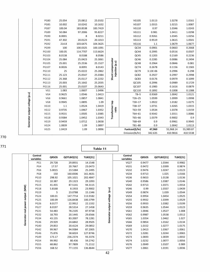
42
PG80 25.054 25.0812 25.0102 VG105 1.0113 1.0278 1.0161
PG85 10.002 10.0242 10.1632 VG107 1.0315 1.0215 1.0087
PG87 100.04 183.8538 183.7419 VG110 0.97 1.0346 1.0243
PG89 50.084 97.2006 95.8227 VG111 0.981 1.0411 1.0298
PG90 8.0001 8 8.0211 VG112 0.9261 1.0345 1.0256
PG91 47.302 20.0123 20.1013 VG113 0.9519 1.0615 1.0501
PG92 214.8 103.6475 104.3625 VG116 1.1 1.0679 1.0677
PG99 100 100.0325 100.1091
Shu
nt
com
pe
nsa
tor
inje
ctio
n (
p.u
)
QC34 0.0901 0.0663 0.2668
PG100 100.05 114.7707 113.6624 QC44 0.2995 0.0516 0.0507
PG103 8.0138 8.0188 8.0586 QC45 0.1203 0.2169 0.2236
PG104 25.084 25.0423 25.3061 QC46 0.2285 0.0086 0.2494
PG105 25.001 25.2536 25.1527 QC48 0.2964 0.0846 0.081
PG107 8.0026 8.0091 8.0143 QC74 0.2678 0.1156 0.1583
PG110 25 25.0222 25.2862 QC79 3.13E-06 0.2996 0.298
PG111 25.123 25.0547 25.0384 QC82 0.2927 0.2997 0.2998
PG112 25.368 25.0117 25.2232 QC83 0.0176 0.0979 0.1099
PG113 25.003 25.1642 25.2035 QC105 0.2996 0.0989 0.1729
PG116 25.001 25.0107 25.0643 QC107 0.1983 0.1616 0.0879
Ge
ne
rato
r o
utp
ut
volt
age
(p
.u)
VG1 1.083 1.0607 1.0496 QC110 0.1892 0.1008 0.1388
VG4 0.9625 1.0546 1.0413
Tran
sfo
rme
r ta
p
ra
tio
T8–5 0.9369 1.0042 1.0121
VG6 0.9661 1.0857 1.0841 T26–25 1.0599 1.0999 1.0998
VG8 0.9945 1.0895 1.09 T30–17 1.0922 1.0182 1.0275
VG10 1.1 1.0524 1.0419 T38–37 1.0731 1.0265 1.0315
VG12 0.9735 1.0467 1.0352 T63–59 1.0534 1.0378 1.0159
VG15 0.9531 1.0505 1.0385 T64–61 0.9342 1.0311 1.0086
VG18 0.9384 1.0452 1.0343 T65–66 1.0379 0.9002 0.9
VG19 0.9459 1.0712 1.0658 T68–69 0.9 0.9961 0.9945
VG24 1.0839 1.09 1.0897 T81–80 0.9 1.0042 1.0113
VG25 1.0419 1.09 1.0896 Fuelcost($/hr) 47,960 55,968.14 55,989.87
Emission(lb/hr) 342.635 410.9816 410.5538
770
771
Control variables
QRSOS QOTLBO[21] TLBO[21] Control
variables QRSOS QOTLBO[21] TLBO[21]
Ge
ne
rato
r re
al p
ow
er
ou
tpu
t (
MW
)
PG1 29.728 29.8931 14.1548
Ge
ne
rato
r o
utp
ut
volt
age
(p
.u)
VG27 0.9477 1.0344 0.9982
PG4 17.57 20.7667 23.0473 VG31 0.9472 1.0399 0.9874
PG6 5.0015 23.5384 25.2495 VG32 0.9476 1.0247 1.0123
PG8 150 160.8306 161.4631 VG34 0.9713 1.025 1.0166
PG10 298.92 105.1021 202.4847 VG36 0.9653 1.0138 1.0136
PG12 10.387 29.1323 29.1093 VG40 0.9586 1.0387 1.0146
PG15 41.455 87.5141 94.3115 VG42 0.9713 1.0371 1.0554
PG18 5.8168 8.1933 23.9002 VG46 0.99 1.0337 1.0439
PG19 5 23.0788 15.1346 VG49 0.9874 1.039 1.0544
PG24 100.01 147.7714 113.9182 VG54 0.9954 1.0454 1.0525
PG25 100.09 126.8438 100.3799 VG55 0.9932 1.0399 1.0529
PG26 8.0177 22.9912 22.1332 VG56 0.9933 1.0382 1.0199
PG27 8.0197 28.5314 27.1458 VG59 0.9635 1.0544 1.0123
PG31 54.483 78.2105 87.9738 VG61 1.0046 1.0527 1.008
PG32 18.793 20.1445 29.6566 VG62 0.9987 1.0538 1.0512
PG34 43.155 83.2007 78.1281 VG65 1.0354 1.0462 1.027
PG36 29.929 24.6842 28.9505 VG66 0.9854 1.0162 1.0134
PG40 29.853 20.4124 29.0852 VG69 1.0152 1.0277 1.0175
PG42 99.967 94.9384 87.2005 VG70 1.0413 1.0367 1.0061
PG46 75.876 58.6024 127.8746 VG72 1.0281 1.0244 1.0065
PG49 173.17 236.2374 93.3376 VG73 1.0693 1.0039 1.0032
PG54 99.992 80.436 59.2742 VG74 1.0232 1.0077 1.0056
PG55 68.862 97.7809 71.2112 VG76 1.0049 1.0107 0.989
PG56 168.52 77.1155 136.8644 VG77 1.0061 1.0191 1.0036
Table 11
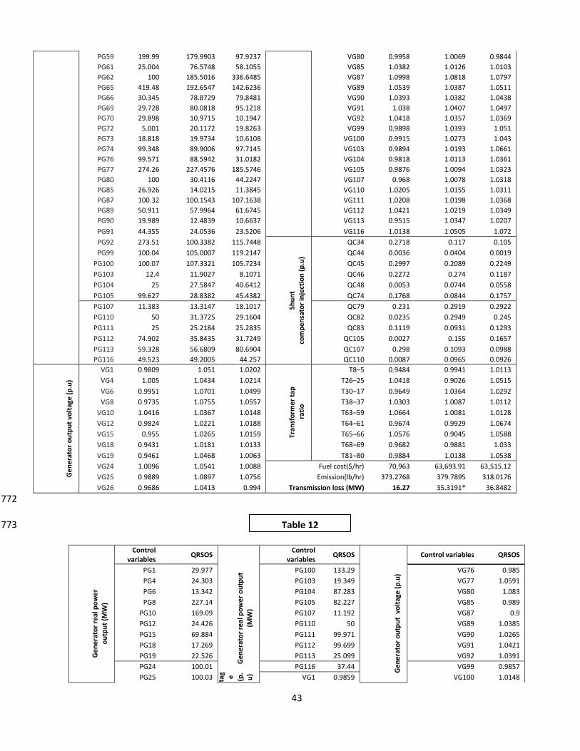
43
PG59 199.99 179.9903 97.9237 VG80 0.9958 1.0069 0.9844
PG61 25.004 76.5748 58.1055 VG85 1.0382 1.0126 1.0103
PG62 100 185.5016 336.6485 VG87 1.0998 1.0818 1.0797
PG65 419.48 192.6547 142.6236 VG89 1.0539 1.0387 1.0511
PG66 30.345 78.8729 79.8481 VG90 1.0393 1.0382 1.0438
PG69 29.728 80.0818 95.1218 VG91 1.038 1.0407 1.0497
PG70 29.898 10.9715 10.1947 VG92 1.0418 1.0357 1.0369
PG72 5.001 20.1172 19.8263 VG99 0.9898 1.0393 1.051
PG73 18.818 19.9734 10.6108 VG100 0.9915 1.0273 1.043
PG74 99.348 89.9006 97.7145 VG103 0.9894 1.0193 1.0661
PG76 99.571 88.5942 31.0182 VG104 0.9818 1.0113 1.0361
PG77 274.26 227.4576 185.5746 VG105 0.9876 1.0094 1.0323
PG80 100 30.4116 44.2247 VG107 0.968 1.0078 1.0318
PG85 26.926 14.0215 11.3845 VG110 1.0205 1.0155 1.0311
PG87 100.32 100.1543 107.1638 VG111 1.0208 1.0198 1.0368
PG89 50.911 57.9964 61.6745 VG112 1.0421 1.0219 1.0349
PG90 19.989 12.4839 10.6637 VG113 0.9515 1.0347 1.0207
PG91 44.355 24.0536 23.5206 VG116 1.0138 1.0505 1.072
PG92 273.51 100.3382 115.7448
Shu
nt
co
mp
en
sato
r in
ject
ion
(p
.u)
QC34 0.2718 0.117 0.105
PG99 100.04 105.0007 119.2147 QC44 0.0036 0.0404 0.0019
PG100 100.07 107.3321 105.7234 QC45 0.2997 0.2089 0.2249
PG103 12.4 11.9027 8.1071 QC46 0.2272 0.274 0.1187
PG104 25 27.5847 40.6412 QC48 0.0053 0.0744 0.0558
PG105 99.627 28.8382 45.4382 QC74 0.1768 0.0844 0.1757
PG107 11.383 13.3147 18.1017 QC79 0.231 0.2919 0.2922
PG110 50 31.3725 29.1604 QC82 0.0235 0.2949 0.245
PG111 25 25.2184 25.2835 QC83 0.1119 0.0931 0.1293
PG112 74.902 35.8435 31.7249 QC105 0.0027 0.155 0.1657
PG113 59.328 56.6809 80.6904 QC107 0.298 0.1093 0.0988
PG116 49.523 49.2005 44.257 QC110 0.0087 0.0965 0.0926
Ge
ne
rato
r o
utp
ut
volt
age
(p
.u)
VG1 0.9809 1.051 1.0202
Tran
sfo
rme
r ta
p
rat
io
T8–5 0.9484 0.9941 1.0113
VG4 1.005 1.0434 1.0214 T26–25 1.0418 0.9026 1.0515
VG6 0.9951 1.0701 1.0499 T30–17 0.9649 1.0364 1.0292
VG8 0.9735 1.0755 1.0557 T38–37 1.0303 1.0087 1.0112
VG10 1.0416 1.0367 1.0148 T63–59 1.0664 1.0081 1.0128
VG12 0.9824 1.0221 1.0188 T64–61 0.9674 0.9929 1.0674
VG15 0.955 1.0265 1.0159 T65–66 1.0576 0.9045 1.0588
VG18 0.9431 1.0181 1.0133 T68–69 0.9682 0.9881 1.033
VG19 0.9461 1.0468 1.0063 T81–80 0.9884 1.0138 1.0538
VG24 1.0096 1.0541 1.0088 Fuel cost($/hr) 70,963 63,693.91 63,515.12
VG25 0.9889 1.0897 1.0756 Emission(lb/hr) 373.2768 379.7895 318.0176
VG26 0.9686 1.0413 0.994 Transmission loss (MW) 16.27 35.3191* 36.8482
772
773
Control variables
QRSOS Control
variables QRSOS Control variables QRSOS
Ge
ne
rato
r re
al p
ow
er
o
utp
ut
(MW
)
PG1 29.977
Ge
ne
rato
r re
al p
ow
er
ou
tpu
t (M
W)
PG100 133.29
Ge
ne
rato
r o
utp
ut
vo
ltag
e (
p.u
)
VG76 0.985
PG4 24.303 PG103 19.349 VG77 1.0591
PG6 13.342 PG104 87.283 VG80 1.083
PG8 227.14 PG105 82.227 VG85 0.989
PG10 169.09 PG107 11.192 VG87 0.9
PG12 24.426 PG110 50 VG89 1.0385
PG15 69.884 PG111 99.971 VG90 1.0265
PG18 17.269 PG112 99.699 VG91 1.0421
PG19 22.526 PG113 25.099 VG92 1.0391
PG24 100.01 PG116 37.44 VG99 0.9857
PG25 100.03 Ge
ne
rat
or
ou tp ut
vo
l
tag e
(p.
u) VG1 0.9859 VG100 1.0148
Table 12
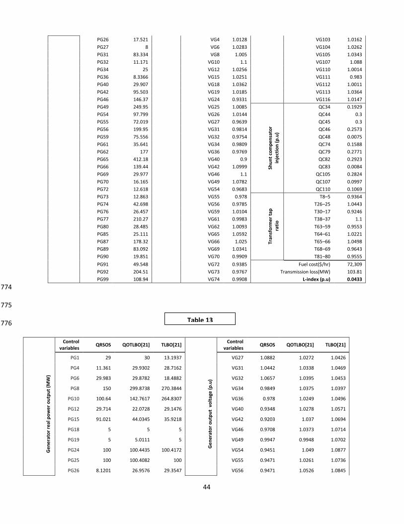
44
PG26 17.521 VG4 1.0128 VG103 1.0162
PG27 8 VG6 1.0283 VG104 1.0262
PG31 83.334 VG8 1.005 VG105 1.0343
PG32 11.171 VG10 1.1 VG107 1.088
PG34 25 VG12 1.0256 VG110 1.0014
PG36 8.3366 VG15 1.0251 VG111 0.983
PG40 29.907 VG18 1.0362 VG112 1.0011
PG42 95.503 VG19 1.0185 VG113 1.0364
PG46 146.37 VG24 0.9331 VG116 1.0147
PG49 249.95 VG25 1.0085
Shu
nt
com
pe
nsa
tor
in
ject
ion
(p
.u)
QC34 0.1929
PG54 97.799 VG26 1.0144 QC44 0.3
PG55 72.019 VG27 0.9639 QC45 0.3
PG56 199.95 VG31 0.9814 QC46 0.2573
PG59 75.556 VG32 0.9754 QC48 0.0075
PG61 35.641 VG34 0.9809 QC74 0.1588
PG62 177 VG36 0.9769 QC79 0.2771
PG65 412.18 VG40 0.9 QC82 0.2923
PG66 139.44 VG42 1.0999 QC83 0.0084
PG69 29.977 VG46 1.1 QC105 0.2824
PG70 16.165 VG49 1.0782 QC107 0.0997
PG72 12.618 VG54 0.9683 QC110 0.1069
PG73 12.863 VG55 0.978
Tran
sfo
rme
r ta
p
rat
io
T8–5 0.9364
PG74 42.698 VG56 0.9785 T26–25 1.0443
PG76 26.457 VG59 1.0104 T30–17 0.9246
PG77 210.27 VG61 0.9983 T38–37 1.1
PG80 28.485 VG62 1.0093 T63–59 0.9553
PG85 25.111 VG65 1.0592 T64–61 1.0221
PG87 178.32 VG66 1.025 T65–66 1.0498
PG89 83.092 VG69 1.0341 T68–69 0.9643
PG90 19.851 VG70 0.9909 T81–80 0.9555
PG91 49.548 VG72 0.9385 Fuel cost($/hr) 72,309
PG92 204.51 VG73 0.9767 Transmission loss(MW) 103.81
PG99 108.94 VG74 0.9908 L-index (p.u) 0.0433
774
775
776
Control variables
QRSOS QOTLBO[21] TLBO[21] Control
variables QRSOS QOTLBO[21] TLBO[21]
Ge
ne
rato
r re
al p
ow
er
ou
tpu
t (M
W)
PG1 29 30 13.1937
Ge
ne
rato
r o
utp
ut
vo
ltag
e (
p.u
)
VG27 1.0882 1.0272 1.0426
PG4 11.361 29.9302 28.7162 VG31 1.0442 1.0338 1.0469
PG6 29.983 29.8782 18.4882 VG32 1.0657 1.0395 1.0453
PG8 150 299.8738 270.3844 VG34 0.9849 1.0375 1.0397
PG10 100.64 142.7617 264.8307 VG36 0.978 1.0249 1.0496
PG12 29.714 22.0728 29.1476 VG40 0.9348 1.0278 1.0571
PG15 91.021 44.0345 35.9218 VG42 0.9203 1.037 1.0694
PG18 5 5 5 VG46 0.9708 1.0373 1.0714
PG19 5 5.0111 5 VG49 0.9947 0.9948 1.0702
PG24 100 100.4435 100.4172 VG54 0.9451 1.049 1.0877
PG25 100 100.4082 100 VG55 0.9471 1.0261 1.0736
PG26 8.1201 26.9576 29.3547 VG56 0.9471 1.0526 1.0845
Table 13
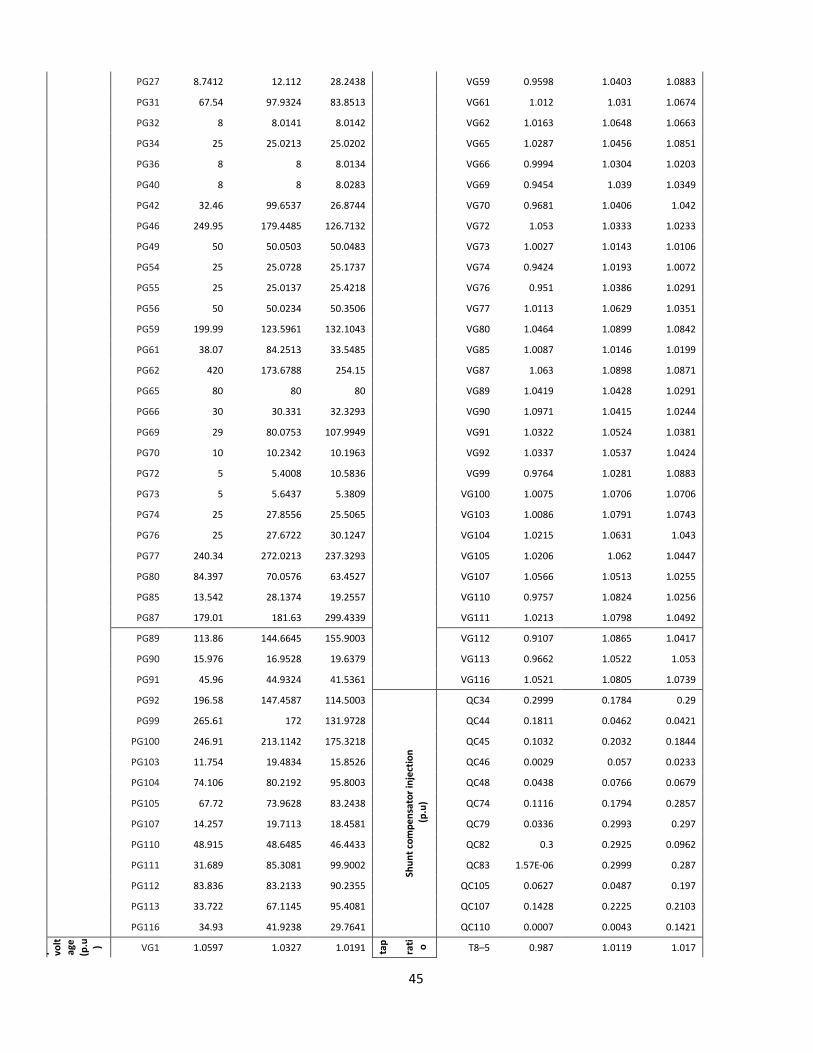
45
PG27 8.7412 12.112 28.2438 VG59 0.9598 1.0403 1.0883
PG31 67.54 97.9324 83.8513 VG61 1.012 1.031 1.0674
PG32 8 8.0141 8.0142 VG62 1.0163 1.0648 1.0663
PG34 25 25.0213 25.0202 VG65 1.0287 1.0456 1.0851
PG36 8 8 8.0134 VG66 0.9994 1.0304 1.0203
PG40 8 8 8.0283 VG69 0.9454 1.039 1.0349
PG42 32.46 99.6537 26.8744 VG70 0.9681 1.0406 1.042
PG46 249.95 179.4485 126.7132 VG72 1.053 1.0333 1.0233
PG49 50 50.0503 50.0483 VG73 1.0027 1.0143 1.0106
PG54 25 25.0728 25.1737 VG74 0.9424 1.0193 1.0072
PG55 25 25.0137 25.4218 VG76 0.951 1.0386 1.0291
PG56 50 50.0234 50.3506 VG77 1.0113 1.0629 1.0351
PG59 199.99 123.5961 132.1043 VG80 1.0464 1.0899 1.0842
PG61 38.07 84.2513 33.5485 VG85 1.0087 1.0146 1.0199
PG62 420 173.6788 254.15 VG87 1.063 1.0898 1.0871
PG65 80 80 80 VG89 1.0419 1.0428 1.0291
PG66 30 30.331 32.3293 VG90 1.0971 1.0415 1.0244
PG69 29 80.0753 107.9949 VG91 1.0322 1.0524 1.0381
PG70 10 10.2342 10.1963 VG92 1.0337 1.0537 1.0424
PG72 5 5.4008 10.5836 VG99 0.9764 1.0281 1.0883
PG73 5 5.6437 5.3809 VG100 1.0075 1.0706 1.0706
PG74 25 27.8556 25.5065 VG103 1.0086 1.0791 1.0743
PG76 25 27.6722 30.1247 VG104 1.0215 1.0631 1.043
PG77 240.34 272.0213 237.3293 VG105 1.0206 1.062 1.0447
PG80 84.397 70.0576 63.4527 VG107 1.0566 1.0513 1.0255
PG85 13.542 28.1374 19.2557 VG110 0.9757 1.0824 1.0256
PG87 179.01 181.63 299.4339 VG111 1.0213 1.0798 1.0492
PG89 113.86 144.6645 155.9003 VG112 0.9107 1.0865 1.0417
PG90 15.976 16.9528 19.6379 VG113 0.9662 1.0522 1.053
PG91 45.96 44.9324 41.5361 VG116 1.0521 1.0805 1.0739
PG92 196.58 147.4587 114.5003
Shu
nt
com
pe
nsa
tor
inje
ctio
n
(p
.u)
QC34 0.2999 0.1784 0.29
PG99 265.61 172 131.9728 QC44 0.1811 0.0462 0.0421
PG100 246.91 213.1142 175.3218 QC45 0.1032 0.2032 0.1844
PG103 11.754 19.4834 15.8526 QC46 0.0029 0.057 0.0233
PG104 74.106 80.2192 95.8003 QC48 0.0438 0.0766 0.0679
PG105 67.72 73.9628 83.2438 QC74 0.1116 0.1794 0.2857
PG107 14.257 19.7113 18.4581 QC79 0.0336 0.2993 0.297
PG110 48.915 48.6485 46.4433 QC82 0.3 0.2925 0.0962
PG111 31.689 85.3081 99.9002 QC83 1.57E-06 0.2999 0.287
PG112 83.836 83.2133 90.2355 QC105 0.0627 0.0487 0.197
PG113 33.722 67.1145 95.4081 QC107 0.1428 0.2225 0.2103
PG116 34.93 41.9238 29.7641 QC110 0.0007 0.0043 0.1421
Ge
ne
rat
or
ou
tp
ut
volt
age
(p.u ) VG1 1.0597 1.0327 1.0191 Tra
nsf
orm
er
tap
rati o
T8–5 0.987 1.0119 1.017
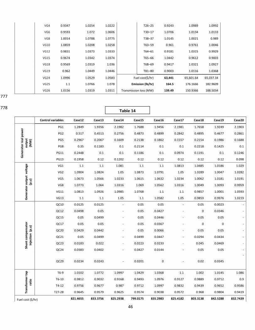
46
VG4 0.9347 1.0254 1.0222 T26–25 0.9243 1.0989 1.0992
VG6 0.9593 1.072 1.0606 T30–17 1.0706 1.0134 1.0133
VG8 1.0014 1.0788 1.0775 T38–37 1.0145 1.0021 0.989
VG10 1.0859 1.0208 1.0258 T63–59 0.961 0.9761 1.0046
VG12 0.9831 1.0373 1.0333 T64–61 0.9181 1.0315 0.9929
VG15 0.9674 1.0342 1.0374 T65–66 1.0442 0.9612 0.9003
VG18 0.9569 1.0319 1.036 T68–69 0.9417 1.0321 1.0927
VG19 0.962 1.0449 1.0446 T81–80 0.9003 1.0116 1.0368
VG24 1.0996 1.0529 1.0583 Fuel cost($/hr) 63,441 65,601.64 65,037.34
VG25 1.1 1.0766 1.078 Emission (lb/hr) 164.5 176.1666 182.9609
VG26 1.0156 1.0319 1.0311 Transmission loss (MW) 139.49 150.9366 188.5034
777
778
Control variables Case12 Case13 Case14 Case15 Case16 Case17 Case18 Case19 Case20
Ge
ne
rato
r re
al p
ow
er
ou
tpu
t
(MW
)
PG1 1.2849 1.9356 2.1982 1.7688 1.9456 2.1981 1.7658 1.9249 2.1903
PG2 0.517 0.4513 0.2756 0.4873 0.4899 0.2842 0.4895 0.4677 0.2861
PG5 0.2967 0.2067 0.1609 0.2138 0.1862 0.1557 0.2154 0.1986 0.1688
PG8 0.35 0.1183 0.1 0.2114 0.1 0.1 0.2218 0.1425 0.1
PG11 0.2448 0.1 0.1 0.1186 0.1 0.0974 0.1191 0.1 0.1246
PG13 0.1958 0.12 0.1202 0.12 0.12 0.12 0.12 0.12 0.098
Ge
ne
rato
r o
utp
ut
vo
ltag
e
(p.u
)
VG1 1.1 1.1 1.081 1.1 1.1 1.0813 1.0485 1.0186 1.029
VG2 1.0904 1.0824 1.05 1.0873 1.0791 1.05 1.0289 1.0047 1.0282
VG5 1.0673 1.0566 1.0233 1.0615 1.0632 1.0234 1.0062 1.0181 1.0191
VG8 1.0773 1.064 1.0316 1.069 1.0562 1.0316 1.0049 1.0093 0.9959
VG11 1.0813 1.0926 1.0985 1.0768 1.1 1.1 0.9857 1.0001 1.0593
VG13 1.1 1.1 1.05 1.1 1.0582 1.05 0.9859 0.9976 1.0219
Shu
nt
com
pe
nsa
tor
in
ject
ion
(p
.u)
QC10 0.0125 0.0125 - 0.05 0.05 - 0.05 0.0023 -
QC12 0.0498 0.05 - 0.05 0.0427 - 0 0.0346 -
QC15 0.05 0.0499 - 0.05 0.0446 - 0.05 0.05 -
QC17 0.05 0.05 - 0.05 0.0367 - 0 0 -
QC20 0.0429 0.0442 - 0.05 0.0066 - 0.05 0.05 -
QC21 0.05 0.0499 - 0.0499 0.0447 - 0.0294 0.0434 -
QC23 0.0183 0.022 - 0.0223 0.0233 - 0.045 0.0469 -
QC24 0.0383 0.0402 - 0.0427 0.0144 - 0.05 0.05 -
QC29 0.0234 0.0243 - 0.0201 0 - 0.02 0.0345
-
Tran
sfo
rme
r ta
p
rati
o
T6-9 1.0102 1.0772 1.0997 1.0429 1.0368 1.1 1.002 1.0145 1.086
T6-10 0.9812 0.9032 0.9168 0.9493 1.0976 0.9127 0.9889 0.9712 0.9
T4-12 0.9756 0.9677 0.987 0.9712 1.0997 0.9832 0.9439 0.9652 0.9586
T27-28 0.9645 0.9579 0.9625 0.9574 0.9038 0.9572 0.968 0.9804 0.9419
Fuel cost ($/hr) 821.4655 833.3756 825.2938 799.0175 835.2983 825.4182 803.3138 842.5288 832.7439
Table 14
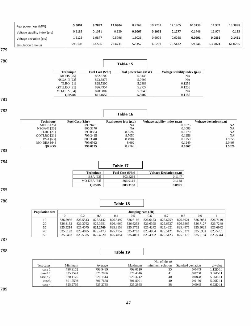
47
Real power loss (MW) 5.5002 9.7887 12.0904 8.7768 10.7703 12.1405 10.0139 11.974 13.3898
Voltage stability index (p.u) 0.1185 0.1081 0.129 0.1067 0.1072 0.1277 0.1446 11.974 0.135
Voltage deviation (p.u) 1.6125 1.9877 0.5796 1.5026 0.9079 0.6268 0.0991 0.0832 0.1461
Simulation time (s) 59.6103 62.566 72.4231 52.352 68.203 76.5432 59.246 63.2024 61.0255
779
780
Technique Fuel Cost ($/hr) Real power loss (MW) Voltage stability index (p.u)
MOHS [25] 832.6709 5.3143 NA NSGA-II [23] 823.8875 5.7699 NA
TLBO [21] 828.5300 5.2883 0.1259
QOTLBO [21] 826.4954 5.2727 0.1255 MO-DEA [64] 820.8802 5.5949 NA
QRSOS 821.4655 5.5002 0.1185
781
782
Technique Fuel Cost ($/hr) Real power loss (p.u) Voltage stability index (p.u) Voltage deviation (p.u) MOHS [25] 799.9401 NA 0.1075 NA
NSGA-II [23] 800.3170 NA 0.1083 NA TLBO [21] 799.8564 8.8592 0.1270 NA
QOTLBO [21] 799.3415 8.7050 0.1256 NA
BSA [63] 800.3340 8.4904 0.1259 1.9855
MO-DEA [64] 799.6912 8.602 0.1249 2.0498 QRSOS 799.0175 8.7768 0.1067 1.5026
783
784
Technique Fuel Cost ($/hr) Voltage Deviation (p.u)
BSA [63] 803.4294 0.1147
MO-DEA [64] 803.9116 0.1158
QRSOS 803.3138 0.0991
785
786
Population size Jumping rate (JR)
0.1 0.2 0.3 0.4 0.5 0.6 0.7 0.8 0.9 1
10 826.5956 826.5543 826.5142 826.5492 826.6166 826.6473 826.6759 826.6921 826.7051 826.7149 20 826.4182 826.3762 826.3651 826.4960 826.6253 826.6395 826.6627 826.6863 826.7127 826.7248
30 825.5214 825.4075 825.2760 825.3153 825.3752 825.4242 825.4621 825.4875 825.5023 825.6942
40 825.5193 825.4695 825.4473 825.4752 825.4763 825.4954 825.5121 825.5274 825.5331 825.5781 50 825.5403 825.5325 825.4620 825.4854 825.4891 825.4902 825.5123 825.5179 825.5194 825.5344
787
788
Test cases Minimum Average Maximum
No. of hits to
minimum solution Standard deviation p-value
case 1 798.9152 798.9439 799.0110 35 0.0443 1.12E-10
case2.1 825.2541 825.2866 825.4346 41 0.0700 3.66E-11 case 2.2 920.1125 920.1514 920.3242 40 0.0828 5.96E-11
case3 801.7593 801.7668 801.8001 40 0.0160 5.96E-11
case 4 825.2769 825.2785 825.2865 38 0.0045 6.92E-11
789
Table 15
Table 16
Table 17
Table 18
Table 19
Recommended