Noname manuscript No.(will be inserted by the editor)
Answering Pattern Match Queries in Large GraphDatabases Via Graph Embedding∗
Lei Zou · Lei Chen · M. Tamer Ozsu · Dongyan Zhao
the date of receipt and acceptance should be inserted later
Abstract The growing popularity of graph databaseshas generated interesting data management problems,such as subgraph search, shortest path query, reacha-bility verification, and pattern matching. Among these,a pattern match query is more flexible compared toa subgraph search and more informative compared toa shortest path or a reachability query. In this paper,we address distance-based pattern match queries over alarge data graph G. Due to the huge search space, weadopt a filter-and-refine framework to answer a patternmatch query over a large graph. We first find a set ofcandidate matches by a graph embedding technique andthen evaluate these to find the exact matches. Extensiveexperiments confirm the superiority of our method.
1 Introduction
As one of the most popular and powerful representa-tions, graphs have been used to model many appli-cation data, such as social networks, biological net-works, and World Wide Web. In order to conduct effec-tive analysis over graphs, various types of queries have
Extended version of paper “Distance-Join: Pattern Match Query
In a Large Graph Database” that was presented in the Proceed-ing of 35th International Conference on Very Large Databases
(VLDB), pages 886-897, 2009.
Lei Zou , Dongyan Zhao
Peking University, Beijing, China
E-mail: zoulei,[email protected]
Lei ChenHong Kong University of Science and Technology, Hong Kong
E-mail: [email protected]
M. Tamer Ozsu
University of Waterloo, Waterloo, CanadaE-mail: [email protected]
been investigated, such as shortest path query [9,18,7], reachability query [9,29,27,5], and subgraph query[24,34,6,17,31,36,15,25]. These are all interesting, butin this paper, we focus on pattern match queries, sincethey are more flexible than subgraph queries and moreinformative than simple shortest path or reachabilityqueries. Specifically, a pattern match query searchesover a large labeled graph to look for the existenceof a pattern graph in a large data graph. A patternmatch query is different from subgraph search in thatit only specifies the vertex labels and connection con-straints between vertices. In other words, a patternmatch query emphasizes the connectivity between la-beled vertices rather than checking subgraph isomor-phism as subgraph search does.
In this paper, we propose a distance-based patternmatch query, which is defined as follows: given a largegraph G, a query graph Q with n vertices and a param-eter δ, n vertices in G match Q iff: (1) these n verticesin G have the same labels as the corresponding verticesin Q, and (2) for any two adjacent vertices vi and vj
in Q (i.e., there is an edge between vi and vj in Q and1 ≤ i, j ≤ n), the distance between two correspondingvertices in G is no larger than δ. We need to find allmatches of Q in G. In this work, we use the shortestpath to measure the distance between two vertices, butour approach is not restricted to this distance function,and can be applied to other metric distance functionsas well. Note that, for ease of presentation, we use theterm “pattern match” instead of “distance-based pat-tern match” in the rest of this paper, when the contextis clear.
A key problem of pattern match queries is hugesearch space. Given a query Q with n vertices, for eachvertex vi in Q, we first find a list of vertices in datagraph G that have the same labels as that of vi. Then,
2
for each pair of adjacent vertices vi and vj in Q, weneed to find all matching pairs in G whose distancesare less than δ. This is called an edge query. To an-swer an edge query, we need to conduct a distance-based join operation between two lists of matching ver-tices corresponding to vi and vj in G. Therefore, findingpattern Q in G requires a sequence of distance-basedjoin operations, which is very costly for large graphs.In order to answer pattern match queries efficiently, weadopt the filter-and-refine framework. Specifically, weneed efficient pruning strategies to reduce the searchspace. Although many effective pruning techniques havebeen proposed for subgraph search (e.g., [24,34,6,17,31,36,15,25]), they can not be applied to pattern matchqueries since these pruning rules are based on the nec-essary condition of subgraph isomorphism. We proposea novel and effective method to reduce the search spacesignificantly. Specifically, we transform vertices into pointsin a vector space via graph embedding methods, con-verting a pattern match query into a distance-basedmulti-way join problem over the vector space to findcandidate matches. In order to reduce the join cost, wepropose several pruning rules to reduce the search spacefurther, and propose a cost model to guide the selectionof the join order to process multi-way join efficiently.
During the refinement process, we adopt 2-hop dis-tance label [9] to compute the shortest path distancefor each candidate match. Unfortunately, finding theoptimal 2-hop distance-aware labeling (i.e., one wherethe size of 2-hop distance-aware labels is minimized) isa NP-hard problem [9]. Although a heuristic method tocompute 2-hop distance-aware labels in a large directedgraph has been proposed [7], this method cannot workwell in a large undirected graph. We will discuss thismethod in detail in Section 2. In this paper, we proposea betweenness (Definition 3) estimation-based methodto guide 2-hop distance-aware center selection. Exten-sive experiments on both real and synthetic datasetsconfirm the efficiency of our method.
To summarize, in this work, we make the followingcontributions:
1) We propose a general framework for handlingpattern match queries over a large graph. Specifically,we adopt a filter-and-refine framework to answer pat-tern match queries. During filtering, we map verticesinto vectors via an embedding method and conductdistance-based multi-way join over the vector space.
2) We design an efficient distance-based join algo-rithm (D-join for short) for an edge query in the con-verted vector space, which well utilizes the block nestedloop join and hash join techniques to handle the highdimensional vector space. We also develop an effectivecost model to estimate the cost of each join operation,
based on which we can select the most efficient joinorder to reduce the cost of multi-way join.
3) In order to address the high complexity of of-fline processing, we propose a graph partitioning-basedmethod and bi-level version of D-join algorithm, calledbD-join.
4) In order to enable shortest path distance compu-tation efficiently, we propose betweenness estimation-based method to compute 2-hop distance labels in alarge graph.
5) In order to answer an approximate subgraph query(Definition 9), we first transform it into a distance-based pattern match query. Then, we find candidates byD-join algorithm. Finally, for each candidate, we verifywhether it is an approximate subgraph match (Defini-tion 8).
6) Finally, we conduct extensive experiments withreal and synthetic data to evaluate the proposed ap-proaches.
The rest of this paper is organized as follows. Wediscuss the related work in Section 2. Our frameworkis presented in Section 3. We propose betweenness esti-mation-based method to compute 2-hop distance labelsin Section 4. The offline process is discussed in Section5. We discuss the neighbor area pruning technique inSection 6, and a distance-based join algorithm for anedge query and its cost model in Section 7. Section7 also presents a distance-based multi-way join algo-rithm for a pattern match query and join order selectionmethod. In Section 8, we propose a graph partition-based method to reduce the cost of offline processingand the bD-join algorithm. In Section 9, we proposea distance-join based solution to answer approximatesubgraph queries. We study our methods by experi-ments in Section 10. Section 11 concludes this paper.
2 Background and Related Work
Let G = 〈V,E〉 be a graph where V is the set of verticesand E is the set of edges. Given two vertices u1 and u2
in G, a reachability query verifies if there exists a pathfrom u1 to u2, and a distance query returns the shortestpath distance between u1 and u2 [9]. These are well-studied problems, with a number of vertex labeling-based solutions [9]. A family of labeling techniques havebeen proposed to answer both reachability and distancequeries. A 2-hop labeling method over a large graphG assigns to each vertex u ∈ V (G) a label L(u) =(Lin(u), Lout(u)), where Lin(u), Lout(u) ⊆ V (G). Ver-tices in Lin(u) and Lout(u) are called centers. There aretwo kinds of 2-hop labeling: 2-hop reachability label-ing (reachability labeling for short) and 2-hop distance
3
labeling (distance labeling for short). For reachabilitylabeling, given any two vertices u1, u2 ∈ V (G), there isa path from u1 to u2 (denoted as u1 → u2), if and onlyif Lout(u1)∩Lin(u2) 6= φ. For distance labeling, we cancompute Distsp(u1, u2) using the following equation.
Distsp(u1, u2) = minDistsp(u1, w) + Distsp(u2, w)|w ∈ (Lout(u1) ∩ Lin(u2))
(1)
where Distsp(u1, u2) is the shortest path distance be-tween vertices u1 and u2. The distances between ver-tices and centers (i.e., Distsp(u1, w) and Distsp(u2, w))are pre-computed and stored. The size of 2-hop labelingis defined as
∑u∈V (G) (|Lin(u)|+ |Lout(u)|), while the
size of 2-hop distance labeling is O(|V (G)||E(G)|1/2)[8]. Thus, according to Equation 1, we need O(|E(G)|1/2)time to compute the shortest path distance by distancelabeling because the average vertex distance label sizeis O(|E(G)|1/2).
Note that, this work focuses on the shortest pathdistance computation. Finding the optimal 2-hop dis-tance labeling is NP-hard [9]. Therefore, a heuristic al-gorithm based on the minimal set-cover problem is pro-posed [9]. Initially, all pairwise shortest paths are com-puted in G (denoted by DG). Then, in each iteration,one vertex w in V (G) is selected as a 2-hop center tomaximize Equation 2.
|D(G,w) ∩DG||Aw|+ |Dw|
(2)
where D(G,w) denotes the shortest paths that are cov-ered by w, and Aw contains all vertices that can reachw and Dw contains all vertices that are reachable fromw. Note that, Aw and Dw are also called the ancestorand descendant clusters of w.
Then, all paths in D(G,w) are removed from DG.This process is iterated until DG = φ, and all selected2-hop centers are returned. According to the 2-hop cen-ters, the corresponding ancestor and descendant clus-ters are built, according to which, a 2-hop label for eachvertex in G is generated. Note that, in order to evaluateEquation 2, all pairwise shortest paths (i.e., DG) needto be kept in memory. Obviously, this requirement isprohibitive for a large graph due to high space com-plexity O(|V (G)|2). Furthermore, also due to high timecomplexity, it is impossible to pre-compute all pairwiseshortest paths in a large graph G in a reasonable time.
There are many proposals for computing reachabil-ity labeling in a large graph (e.g., [27,29]). However,2-hop distance-aware labeling computation in a largegraph has not attracted much attention except for the
work of Cheng and Yu [7], where a large directed graphG is first converted into a directed acyclic graph (DAG)G↓ by removing some vertices in each strongly con-nected component (SCC) of G. These removed verticesare selected as 2-hop centers. Obviously, all shortestpaths that pass through these removed vertices are cov-ered by these selected 2-hop centers. Then, G↓ is par-titioned into two subgraphs, denoted as G> and G⊥,by a set of node-separators Vw. These vertices in Vw
are selected as 2-hop centers as well. All shortest pathsacross G> and G⊥ must be covered by Vw. These twopartitions can be considered separately. If G> is smallenough, the method in [9] can be employed to compute2-hop labels in G>; otherwise, the partition process isrepeated until the 2-hop label in each partition can becomputed by the method in [9] directly. The same pro-cess is followed for G⊥.
Given a 2-hop center w, it is not necessary that Aw
(and Dw) contains all ancestor (and descendant) nodesof w in a directed graph G, or all vertices in an undi-rected graph G. Some pruning methods have been pro-posed for this purpose based on the previously identified2-hop clusters [7].
There are two problems in the method of [7]. Firstly,if G is not a sparse directed graph, there may exist alarge number of strongly connected components (SCC)in G. Consequently, a large number of vertices need tobe removed from G to generate a DAG. This meansthat the size of 2-hop labeling in G is very large. Fur-thermore, if G is an undirected graph, it is impossibleto generate a DAG by removing some vertices in G.Secondly, the proposed pruning methods reduce the re-dundancy and the labeling size, but the pruning strat-egy is based on all previously identified 2-hop clusters.Thus, all previously identified 2-hop clusters need to becached in memory; otherwise, frequent swap-ins/outswill affect the performance dramatically. Furthermore,the cost of redundancy checking is also expensive.
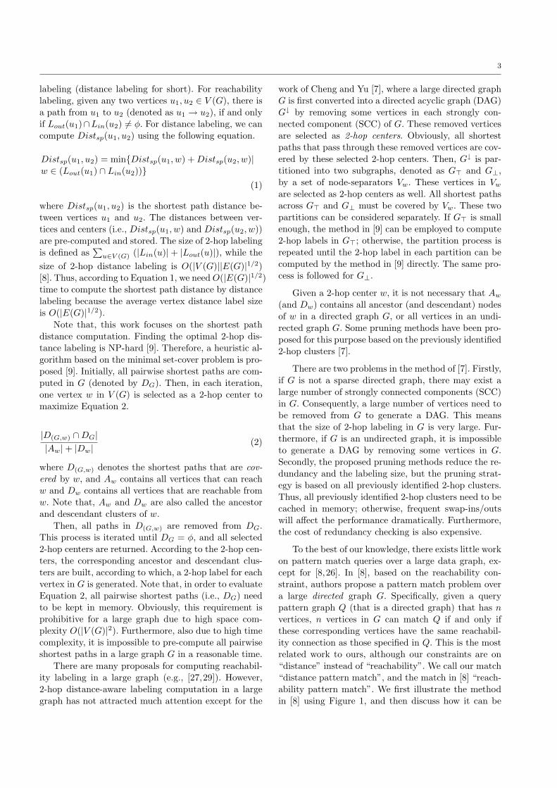
To the best of our knowledge, there exists little workon pattern match queries over a large data graph, ex-cept for [8,26]. In [8], based on the reachability con-straint, authors propose a pattern match problem overa large directed graph G. Specifically, given a querypattern graph Q (that is a directed graph) that has nvertices, n vertices in G can match Q if and only ifthese corresponding vertices have the same reachabil-ity connection as those specified in Q. This is the mostrelated work to ours, although our constraints are on“distance” instead of “reachability”. We call our match“distance pattern match”, and the match in [8] “reach-ability pattern match”. We first illustrate the methodin [8] using Figure 1, and then discuss how it can be
4
extended it to solve our problem and present the short-comings of the extension.
0a 1broot
2c
0b
1b0b
1b2c
0b
( )inL uu ( )outL u
0( )A a 0( )D a 1( )A b 1( )D b 2( )A c 2( )D c
(a) Base Table (b) W-Table
(c ) Cluster-based Index
0 a0a0 a
0 1 , a b0b 2 c1 b1b 1 b
0 1 , a b0b 2 c2 c2c 1 2 , b c
label pair centers0 a
1 2 , b c( , )a b( , )b c
2c2c
0a0a
Fig. 1 R-join
Without loss of generality, assume that there is onlyone directed edge e = (v1, v2) in query Q. Figure 1(a)shows a base table to store all vertex distance labels.For each center wi in graph G, Awi
and Dwiare 2-
hop reachability clusters for wi. Awi and Dwi containall ancestor nodes and descendant nodes of wi in G,respectively, where for every vertex u1 in Awi
, everyvertex u2 in Dwi can be reached via wi. Then, an in-dex structure is built based on these clusters, as shownin Figure 1(c). For each vertex label pair (l1, l2), allcenters wi are stored (in table W-Table), where thereexists at least one vertex labeled l1 (and l2) in A(wi)(and D(wi)). Consider a directed edge e = (v1, v2) inquery Q and assume that the labels of vertices v1 andv2 (in query Q) are ‘a’ and ‘b’, respectively. Accord-ing to W-Table in Figure 1b, we can find centers wi,in which there exists at least a vertex u1 labeled ‘a’ inAwi , and there exists at least a vertex u2 labeled ‘b’in Dwi . For each such center wi, the Cartesian productof vertices labeled ‘a’ in Awi
and vertices labeled ‘b’ inDwi
can form the matches of Q. This operation is calledR-join [8]. In this example, there is only one center a0
that corresponds to vertex label pair (a, b), as shownin Figure 1(b). According to index structure in Figure1(c), F (a0) and T (a0) can be found. When the numberof edges in Q is larger than one, a reachability patternmatch query can be answered by a sequence of R-joins.
2-hop distance labeling has the structure similar to2-hop reachability labeling, we can extend the methodproposed in [8] to answer distance pattern match query.Specifically, in the last step, for each vertex pair (u1, u2)in the Cartesian product, we need to compute dist =Distsp(u1, wi) + Distsp(u2, wi). If dist ≤ δ, (u1, u2) isa match. Note that this step is different from reacha-bility pattern match in [8], in which no distance com-putation is needed. Assume that there are n1 vertices
labeled ‘a’ and n2 vertices labeled ‘b’ in a graph G. Itis clear that the number of distance computations is atleast n1 × n2, which is exactly the same as naive joinprocessing. Therefore, this extension method will notreduce the search space. Thus, the motivation of ourwork is exactly this: is it possible to avoid unnecessarydistance computation to speed up the search efficiency?Several efficient and effective pruning techniques areproposed in this paper.
The best-effect algorithm [26] returns K matcheswith large scores. That algorithm cannot guarantee thatthe k result matches are the k largest over all matches.We cannot extend this method to apply to our problem,since it cannot guarantee the completeness of results. In[11], authors propose ranked twig queries over a largegraph, however, a “twig pattern” is a directed graph,not a general graph.
3 Framework
Definition 1 (Distance-based Pattern Match). Con-sider a data graph G, a connected query graph Q thathas n vertices v1, ..., vn and m edges e1, ..., em, andm parameters δ1, ..., δm. A set of n distinct verticesu1, ..., un in G is said to be a Distance-based Pat-tern Match of Q, if and only if the following conditionshold:1) ∀i, L(ui) = L(vi), where L(ui) (L(vi)) denotes ui’s(vi’s) label; and2) For each edge ej = (vi1 , vi2) in Q, j = 1, ...,m, theshortest path distance between ui1 and ui2 in G is nolarger than δj . We denote the shortest path betweenui1 and ui2 as ui1ui2 .
For ease of presentation, we assume that all distanceconstraint parameters have the same value, i.e., δ =δ1 = ... = δm. The problem that we study in this paperis defined as follows:
Definition 2 (Distance-based Pattern MatchQuery). Consider a data graph G, a connected querygraph Q that has n vertices v1, ..., vn, and a parame-ter δ. A pattern match query finds all matches (Defini-tion 1) of Q over G.
In this paper, we use the terms “match” and “pat-tern match query” instead of “distance-based patternmatch” and “distance-based pattern match query” forsimplicity, when the context is clear.
According to Definition 1, any match is always con-tained in some connected component of G, since Q isconnected. Without loss of generality, we assume that
5
G is connected. If not, we can sequentially perform pat-tern match queries in each connected component of Gto find all matches.
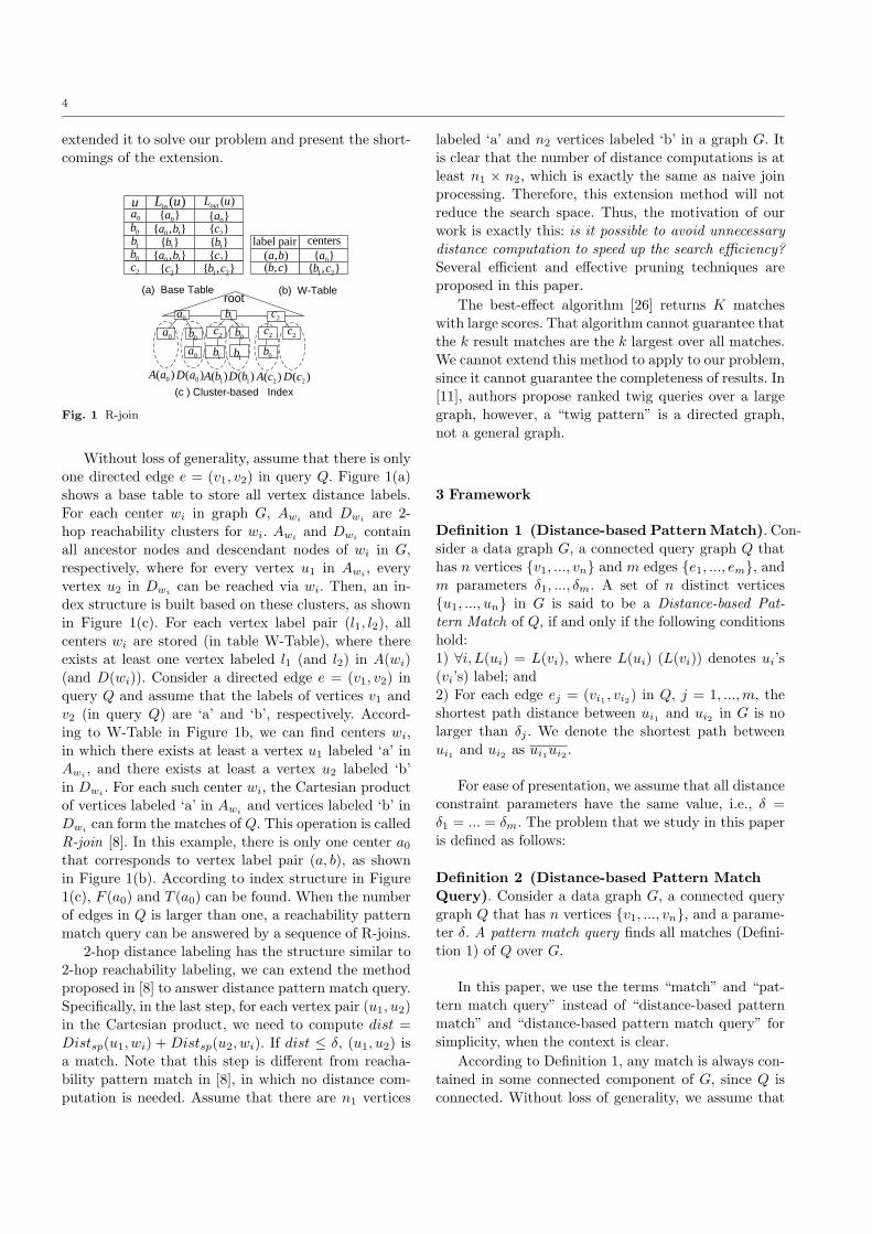
One way of executing the pattern match query (thatwe call naive join processing) is the following. Using thevertex label predicates associated with each vertex vi ofa query graph Q, derive n lists of vertices (R1, . . . , Rn),where each list Ri contains all vertices ui whose labelsare the same as vi’s label (list Ri is said to correspondto a vertex vi in Q). Then, perform a shortest pathdistance-based multi-way join over these lists. Join re-quires the definition of a join order, which, in this case,corresponds to a traversal order in Q. At each traversalstep, the subgraph induced by all visited edges (in Q) isdenoted as Q′. Figure 2 shows a join order (i.e., traver-sal order in Q) of a sample query Q. In the first step,there is only one edge in Q′, thus, the pattern matchquery degrades into an edge query. After the first step,we still need to answer an edge query for each new en-countered edge. It is clear that different join orders willlead to different performance.
a
b c
dQuery Q
NULLa
bab c
ab ca
b cd
Fig. 2 A Join-Order
According to Definition 1, we have to perform short-est path distance computation online. The straightfor-ward solution to reduce the cost is to pre-compute andstore all pairwise shortest path distances (Pre-computemethod). The method is fast, but prohibitive in spaceusage (it needs O(|V (G)|2) space). Graph labeling tech-nique enables the computation of shortest path dis-tance in O(|E(G)|1/2) time, while the space cost is onlyO(|V (G)||E(G)|1/2) [9]. Thus, we adopt the graph la-beling technique to perform shortest path distance com-putation. However, computing the optimal 2-hop dis-tance labels (i.e., the size of 2-hop distance labels isminimized) is NP-hard [9]. In Section 4, we proposea betweenness estimation-based method to compute 2-hop distance-aware labels in a large graph G.
The key problem in naive join processing is its largenumber of distance computations. In order to speed upthe query performance, we need to address two issues:reducing the number of shortest path distance compu-tations, and finding a distance computation method tofind all candidate matches that are more efficient thanshortest path distance computation.
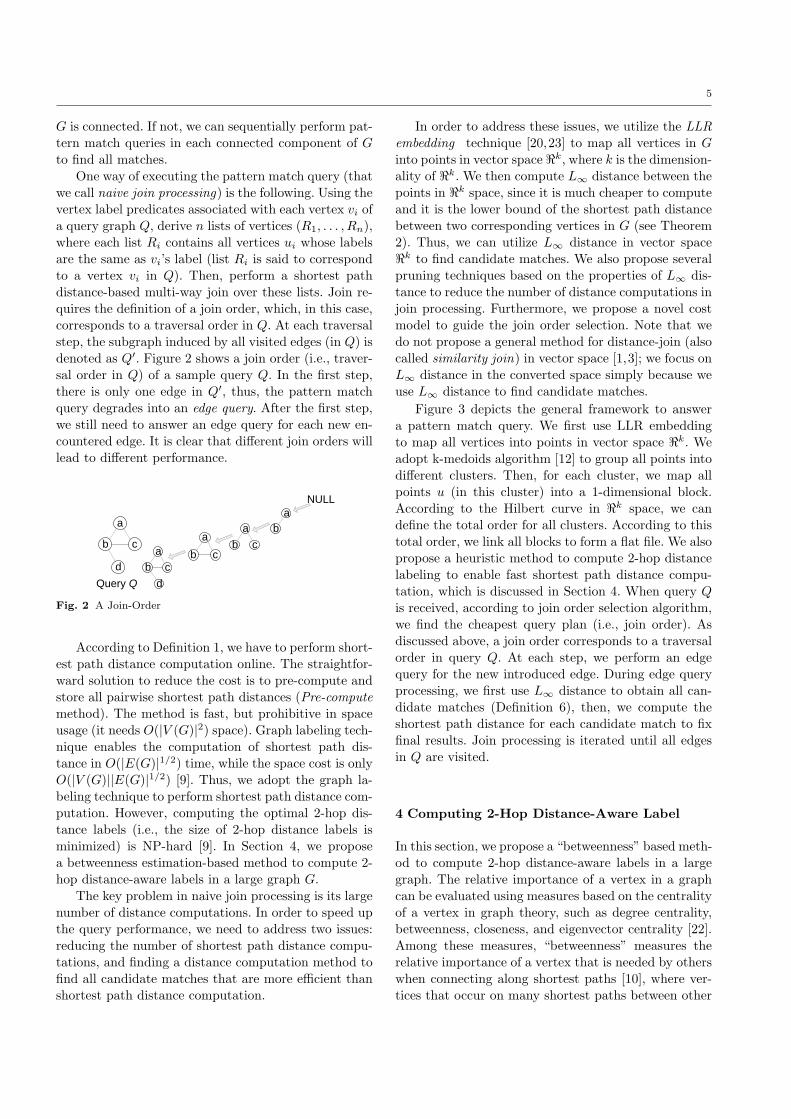
In order to address these issues, we utilize the LLRembedding technique [20,23] to map all vertices in Ginto points in vector space <k, where k is the dimension-ality of <k. We then compute L∞ distance between thepoints in <k space, since it is much cheaper to computeand it is the lower bound of the shortest path distancebetween two corresponding vertices in G (see Theorem2). Thus, we can utilize L∞ distance in vector space<k to find candidate matches. We also propose severalpruning techniques based on the properties of L∞ dis-tance to reduce the number of distance computations injoin processing. Furthermore, we propose a novel costmodel to guide the join order selection. Note that wedo not propose a general method for distance-join (alsocalled similarity join) in vector space [1,3]; we focus onL∞ distance in the converted space simply because weuse L∞ distance to find candidate matches.
Figure 3 depicts the general framework to answera pattern match query. We first use LLR embeddingto map all vertices into points in vector space <k. Weadopt k-medoids algorithm [12] to group all points intodifferent clusters. Then, for each cluster, we map allpoints u (in this cluster) into a 1-dimensional block.According to the Hilbert curve in <k space, we candefine the total order for all clusters. According to thistotal order, we link all blocks to form a flat file. We alsopropose a heuristic method to compute 2-hop distancelabeling to enable fast shortest path distance compu-tation, which is discussed in Section 4. When query Q
is received, according to join order selection algorithm,we find the cheapest query plan (i.e., join order). Asdiscussed above, a join order corresponds to a traversalorder in query Q. At each step, we perform an edgequery for the new introduced edge. During edge queryprocessing, we first use L∞ distance to obtain all can-didate matches (Definition 6), then, we compute theshortest path distance for each candidate match to fixfinal results. Join processing is iterated until all edgesin Q are visited.
4 Computing 2-Hop Distance-Aware Label
In this section, we propose a “betweenness” based meth-od to compute 2-hop distance-aware labels in a largegraph. The relative importance of a vertex in a graphcan be evaluated using measures based on the centralityof a vertex in graph theory, such as degree centrality,betweenness, closeness, and eigenvector centrality [22].Among these measures, “betweenness” measures therelative importance of a vertex that is needed by otherswhen connecting along shortest paths [10], where ver-tices that occur on many shortest paths between other
6
Block Nested Loop Join
Vertices in G
Points in kℜ
LLR Embedding
Blocks in a flat file
Vertex distance labels
Candidate SetCL=(u1, u2)
Answer SetRS=(u1, u2)
Edge Query
Pattern Matching Query
Join Order Selection
Clustering
Cost Estimation
Vertex Lists Ri
Shrunk Vertex Lists Ri
Neighbor Area Pruning
Vertex Labels
Offline
Online
Fig. 3 Framework of Pattern Match Query
u0 u1
u2 u3
u4
5 2 2 51
1 1
(a) Graph G
0u 0 0 1( ) ( ,2),( ,3);inL u w w=1u
1 0 1( ) ( ,2),( ,3);inL u w w=2u 2 0 1( ) ( ,0),( ,1);inL u w w=
3u 3 0 1( ) ( ,1),( ,1);inL u w w=4u
4 0 1( ) ( ,1),( ,1);inL u w w=
2-hop Labelsvertex
0u 0 0 1 2( ) ( ,0),( ,5),( ,3);inL u w w w=
1u1 0 1 2( ) ( ,2),( ,5),( ,3);inL u w w w=
2u 2 0 1 3( ) ( ,3),( ,2),( ,1);inL u w w w=3u
0 2 1 3 , w u w u= =
4u4 0 1 2( ) ( ,3),( ,3),( ,0);inL u w w w=
2-hop Labelsvertex
0 0 1 1 2 4 , , w u w u w u= = =
(b) 2-hop labeling with centers
(c) 2-hop labeling with centers
3 0 1 2( ) ( ,2),( ,3),( ,1);inL u w w w=
Fig. 4 2-hop Labeling With Different 2-hop Centers
vertices have higher betweenness value than those thatdo not.
Definition 3 [10] Given a graph G and a vertex u, ifvertex u occurs on the shortest distance path betweenu1 and u2 (u1 6= u2 6= u), we say that u covers the short-est distance path between u1 and u2. The betweennessof v is defined as follows:
Betweenness(u) =∑
u1 6=u 6=u2∈V
σu1u2(u)σu1u2
(3)
where σu1u2(u) denotes the number of different shortestdistance paths between u1 and u2 that are covered byu; and σu1u2 denotes the number of different shortestdistance paths between u1 and u2.
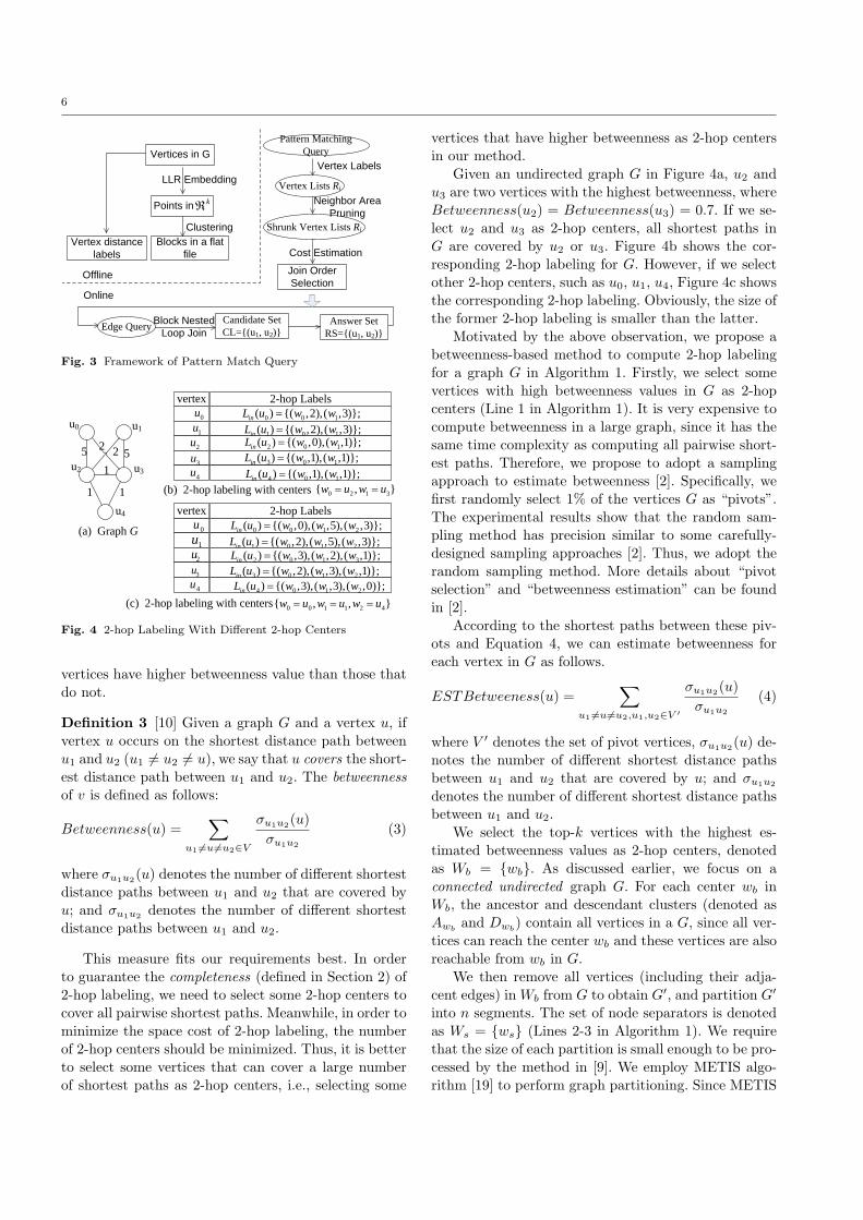
This measure fits our requirements best. In orderto guarantee the completeness (defined in Section 2) of2-hop labeling, we need to select some 2-hop centers tocover all pairwise shortest paths. Meanwhile, in order tominimize the space cost of 2-hop labeling, the numberof 2-hop centers should be minimized. Thus, it is betterto select some vertices that can cover a large numberof shortest paths as 2-hop centers, i.e., selecting some
vertices that have higher betweenness as 2-hop centersin our method.
Given an undirected graph G in Figure 4a, u2 andu3 are two vertices with the highest betweenness, whereBetweenness(u2) = Betweenness(u3) = 0.7. If we se-lect u2 and u3 as 2-hop centers, all shortest paths inG are covered by u2 or u3. Figure 4b shows the cor-responding 2-hop labeling for G. However, if we selectother 2-hop centers, such as u0, u1, u4, Figure 4c showsthe corresponding 2-hop labeling. Obviously, the size ofthe former 2-hop labeling is smaller than the latter.
Motivated by the above observation, we propose abetweenness-based method to compute 2-hop labelingfor a graph G in Algorithm 1. Firstly, we select somevertices with high betweenness values in G as 2-hopcenters (Line 1 in Algorithm 1). It is very expensive tocompute betweenness in a large graph, since it has thesame time complexity as computing all pairwise short-est paths. Therefore, we propose to adopt a samplingapproach to estimate betweenness [2]. Specifically, wefirst randomly select 1% of the vertices G as “pivots”.The experimental results show that the random sam-pling method has precision similar to some carefully-designed sampling approaches [2]. Thus, we adopt therandom sampling method. More details about “pivotselection” and “betweenness estimation” can be foundin [2].
According to the shortest paths between these piv-ots and Equation 4, we can estimate betweenness foreach vertex in G as follows.
ESTBetweeness(u) =∑
u1 6=u 6=u2,u1,u2∈V ′
σu1u2(u)σu1u2
(4)
where V ′ denotes the set of pivot vertices, σu1u2(u) de-notes the number of different shortest distance pathsbetween u1 and u2 that are covered by u; and σu1u2
denotes the number of different shortest distance pathsbetween u1 and u2.
We select the top-k vertices with the highest es-timated betweenness values as 2-hop centers, denotedas Wb = wb. As discussed earlier, we focus on aconnected undirected graph G. For each center wb inWb, the ancestor and descendant clusters (denoted asAwb
and Dwb) contain all vertices in a G, since all ver-
tices can reach the center wb and these vertices are alsoreachable from wb in G.
We then remove all vertices (including their adja-cent edges) in Wb from G to obtain G′, and partition G′
into n segments. The set of node separators is denotedas Ws = ws (Lines 2-3 in Algorithm 1). We requirethat the size of each partition is small enough to be pro-cessed by the method in [9]. We employ METIS algo-rithm [19] to perform graph partitioning. Since METIS
7
performs an edge separator-based partition, we adoptan approach similar to [13] to convert it into a nodeseparator-based partition. Considering one edge sepa-rator e = (u1, u2) that connects two partitions P1 andP2, we shift the partition boundary so that one of u1
and u2 is on the boundary and the other one is in thepartition. The node on the boundary is called a nodeseparator. The choice of node separator depends on thesize of partitions P1 and P2. In order to balance thesize of each partition, we always make the node fromthe large partition a node separator.
We remove all vertices in Wb ∪ Ws and their adja-cent edges from G to obtain G (Line 4). Assume thatthere are m connected components in G. For purposesof presentation, we assume that each connected compo-nent is called a subgraph, denoted Si, i = 1, ...,m. It isclear that m ≥ n, and each subgraph Si is small enoughto be processed by the method in [9], according to thegraph partition method in the second step.
All pairwise shortest paths in G can be classifiedinto two categories, denoted as PathSet1 and PathSet2,where PathSet1 contains all paths that cross at leasttwo subgraphs, and PathSet2 contains the paths thatare constrained in each subgraph.
In order to guarantee the completeness of 2-hop la-beling, the process should consist of two parts, namelyskeleton 2-hop labeling and local 2-hop labeling. The for-mer covers all paths in PathSet1, and the latter coversall paths in PathSet2. For each subgraph Si, we em-ploy the method in [9] to compute local 2-hop labeling(Lines 5-6). The key issue is how to compute skeleton 2-hop labeling. Obviously, all paths in PathSet1 are cov-ered by at least one vertex in Wb ∪Ws. For each vertexw ∈ Wb ∪ Ws, we perform Dijkstra’s algorithm to ob-tain the shortest path tree with root w. The ancestorand descendant clusters for w (denoted as Aw and Dw)contain all vertices in G and their corresponding dis-tances. However, the space cost of this straightforwardapproach is quite high. Some pruning methods based onpreviously identified clusters are proposed in [7]. How-ever, the key problem of this technique is that all previ-ously identified clusters need to be kept in memory forfurther checking. Otherwise, frequent swaps will affectthe performance dramatically, making it prohibitive ina large graph.
An interesting observation is that a large fragmentof shortest paths in PathSet1 are covered by Wb, but|Wb| = k << |Ws|. Therefore, we propose the followingmethod to reduce redundancies in 2-hop clusters: Foreach vertex wb ∈ Wb, Awb
(and Dwb) contains all ver-
tices in G and their corresponding distances (Lines 7-9).However, it is not necessary for Aws
and Dws(ws ∈ Ws)
to contain all vertices in G, since most paths have beencovered by some 2-hop centers in Wb.
Theorem 1 Given a 2-hop center ws ∈ Ws and a ver-tex u in G, if the shortest path between ws and u (de-noted as uws) passes through some vertex wb ∈ Wb, ucan be filtered out from Aws
and Dwswithout affecting
the completeness of 2-hop labeling.
Proof See [37].
According to Theorem 1, we have the following steps.For each 2-hop center wb ∈ Wb, we perform Dijkstra’salgorithm to obtain the shortest path tree with rootwb. The 2-hop cluster for wb ∈ Wb contains all ver-tices in G and the corresponding distances (Lines 7-9).For each 2-hop center ws ∈ Ws, we also perform Dijk-stra’s algorithm to obtain the shortest path tree withroot ws (Line 11). If the shortest path between ws andsome vertex u (denoted as wsu) passes through another2-hop center wb, u can be filtered out from Aws andDws
(Lines 15-16). According to the 2-hop clusters, itis straightforward to obtain the skeleton 2-hop labels(Line 17).
As mentioned earlier, 2-hop label of each vertex con-tains two parts, a local 2-hop label and a skeleton 2-hop,which can be obtained in Lines 5-6 and Lines 7-17 ofAlgorithm 1, respectively. Finally, for each vertex, wecombine the local 2-hop labels and the skeleton 2-hoplabels together (Line 18).
5 Offline Processing For Pattern Match Query
5.1 Graph Embedding Technique
According to LLR embedding technique [20,23], we havethe following embedding process to map all vertices inG into points in a vector space <k, where k is the di-mensionality of the vector space:
1) Let Sn,m be a subset of randomly selected verticesin V (G). We define the distance from u to its closestneighbor in Sn,m as follows:
Dist(u, Sn,m) = minu′∈Sn,mDistsp(u, u′) (5)
2) We select k = O(log2|V (G)|) subsets to formthe set R = S1,1, ..., S1,κ, ..., Sβ,1, ..., Sβ,κ. where κ =O(log|V (G)|) and β = O(log|V (G)|) and k = κ · β =O(log2|V (G)|). Each subset Sn,m (1 ≤ n ≤ β, 1 ≤ m ≤κ) in R has 2n vertices in V (G).
3) The mapping function E : V (G) → <k is definedas follows:
E(u) = [Dist(u, S1,1), ..., Dist(u, S1,κ), ..., Dist(u, Sβ,1),..., Dist(u, Sβ,κ)]
8
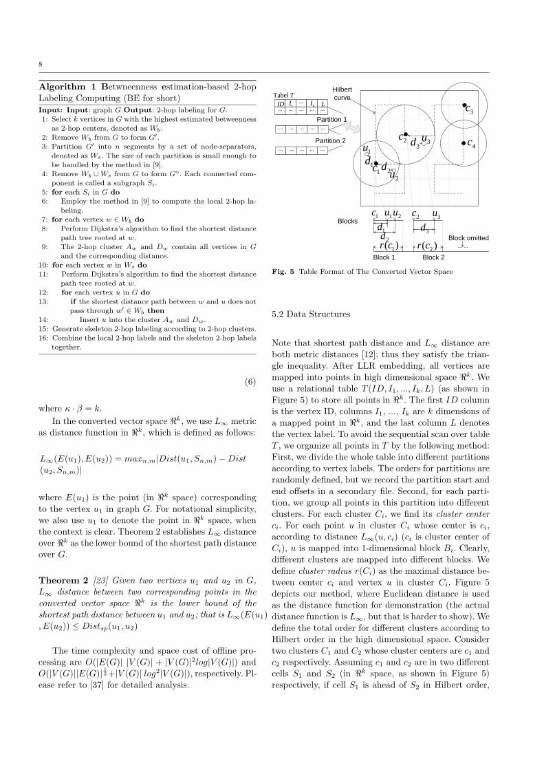
Algorithm 1 Betwneenness estimation-based 2-hopLabeling Computing (BE for short)Input: Input: graph G Output: 2-hop labeling for G.
1: Select k vertices in G with the highest estimated betweenness
as 2-hop centers, denoted as Wb.2: Remove Wb from G to form G′.3: Partition G′ into n segments by a set of node-separators,
denoted as Ws. The size of each partition is small enough to
be handled by the method in [9].
4: Remove Wb ∪Ws from G to form G. Each connected com-ponent is called a subgraph Si.
5: for each Si in G do
6: Employ the method in [9] to compute the local 2-hop la-beling.
7: for each vertex w ∈ Wb do
8: Perform Dijkstra’s algorithm to find the shortest distancepath tree rooted at w.
9: The 2-hop cluster Aw and Dw contain all vertices in G
and the corresponding distance.10: for each vertex w in Ws do
11: Perform Dijkstra’s algorithm to find the shortest distance
path tree rooted at w.12: for each vertex u in G do
13: if the shortest distance path between w and u does notpass through w′ ∈ Wb then
14: Insert u into the cluster Aw and Dw.
15: Generate skeleton 2-hop labeling according to 2-hop clusters.16: Combine the local 2-hop labels and the skeleton 2-hop labels
together.
(6)
where κ · β = k.In the converted vector space <k, we use L∞ metric
as distance function in <k, which is defined as follows:
L∞(E(u1), E(u2)) = maxn,m|Dist(u1, Sn,m)−Dist(u2, Sn,m)|
where E(u1) is the point (in <k space) correspondingto the vertex u1 in graph G. For notational simplicity,we also use u1 to denote the point in <k space, whenthe context is clear. Theorem 2 establishes L∞ distanceover <k as the lower bound of the shortest path distanceover G.
Theorem 2 [23] Given two vertices u1 and u2 in G,L∞ distance between two corresponding points in theconverted vector space <k is the lower bound of theshortest path distance between u1 and u2; that is L∞(E(u1), E(u2)) ≤ Distsp(u1, u2)
The time complexity and space cost of offline pro-cessing are O(|E(G)| |V (G)| + |V (G)|2log|V (G)|) andO(|V (G)||E(G)| 12 +|V (G)| log2|V (G)|), respectively. Pl-ease refer to [37] for detailed analysis.
Block 1 … …
Hilbert curve
Block omitted
Block 2 1( )r c 2( )r c
1c 1u 2u
1d2d 3d
1d1u
1c 2d2u
2c 3u
2c3d 3u
3c
4c
Blocks
…
… … … ……
Tabel T
… … … ……
… … … ……
Partition 1
Partition 2
1I kI LID
Fig. 5 Table Format of The Converted Vector Space
5.2 Data Structures
Note that shortest path distance and L∞ distance areboth metric distances [12]; thus they satisfy the trian-gle inequality. After LLR embedding, all vertices aremapped into points in high dimensional space <k. Weuse a relational table T (ID, I1, ..., Ik, L) (as shown inFigure 5) to store all points in <k. The first ID columnis the vertex ID, columns I1, ..., Ik are k dimensions ofa mapped point in <k, and the last column L denotesthe vertex label. To avoid the sequential scan over tableT , we organize all points in T by the following method:First, we divide the whole table into different partitionsaccording to vertex labels. The orders for partitions arerandomly defined, but we record the partition start andend offsets in a secondary file. Second, for each parti-tion, we group all points in this partition into differentclusters. For each cluster Ci, we find its cluster centerci. For each point u in cluster Ci whose center is ci,according to distance L∞(u, ci) (ci is cluster center ofCi), u is mapped into 1-dimensional block Bi. Clearly,different clusters are mapped into different blocks. Wedefine cluster radius r(Ci) as the maximal distance be-tween center ci and vertex u in cluster Ci. Figure 5depicts our method, where Euclidean distance is usedas the distance function for demonstration (the actualdistance function is L∞, but that is harder to show). Wedefine the total order for different clusters according toHilbert order in the high dimensional space. Considertwo clusters C1 and C2 whose cluster centers are c1 andc2 respectively. Assuming c1 and c2 are in two differentcells S1 and S2 (in <k space, as shown in Figure 5)respectively, if cell S1 is ahead of S2 in Hilbert order,
9
cluster C1 is larger than C2. If c1 and c2 are in the samecell, the order of C1 and C2 is arbitrarily defined.
Note that the maximal size for one cluster (i.e., oneblock) is specified according to the allocated memorysize. In our implementation, we use K-medoids algo-rithm [12] to find clusters. Also note that the clusteringalgorithm is orthogonal to our approach. How to findan optimal clustering in <k is beyond the scope of thispaper. In the following discussion, we assume that clus-tering results are given.
6 Neighbor Area Pruning
To answer a distance pattern match query, we conducta distance-based join over the converted vector space,not the original graph space. Thus, to reduce the costof join processing, the first step is to remove all thepoints that do not qualify for join condition as early aspossible. In this section, we propose an efficient pruningstrategy called neighbor area pruning.
a
b
cb
a
4u
3u1u
2u 5u
c6u
4 2( , )spDist u u δ>
4 1( , )spDist u u δ>
6 3( , )spDist u u δ>
6 4( , )spDist u u δ<
(b) Query Q
1v
2v3v
(a) Shortest Path Distances in graph G
4 is pruned u
a
b c
Fig. 6 Area Neighbor Pruning
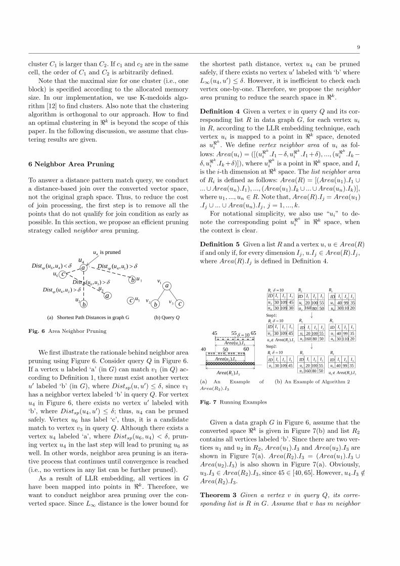
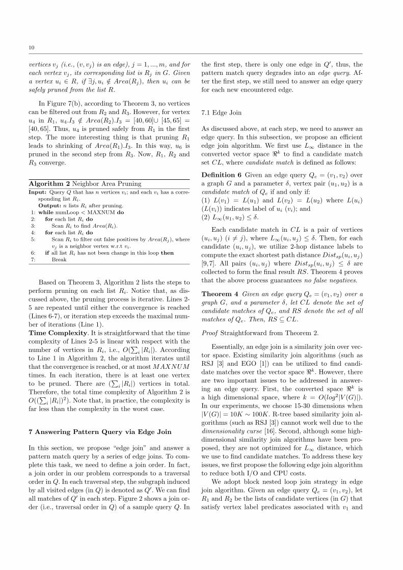
We first illustrate the rationale behind neighbor areapruning using Figure 6. Consider query Q in Figure 6.If a vertex u labeled ‘a’ (in G) can match v1 (in Q) ac-cording to Definition 1, there must exist another vertexu′ labeled ‘b’ (in G), where Distsp(u, u′) ≤ δ, since v1
has a neighbor vertex labeled ‘b’ in query Q. For vertexu4 in Figure 6, there exists no vertex u′ labeled with‘b’, where Distsp(u4, u
′) ≤ δ; thus, u4 can be prunedsafely. Vertex u6 has label ‘c’, thus, it is a candidatematch to vertex v3 in query Q. Although there exists avertex u4 labeled ‘a’, where Distsp(u6, u4) < δ, prun-ing vertex u4 in the last step will lead to pruning u6 aswell. In other words, neighbor area pruning is an itera-tive process that continues until convergence is reached(i.e., no vertices in any list can be further pruned).
As a result of LLR embedding, all vertices in Ghave been mapped into points in <k. Therefore, wewant to conduct neighbor area pruning over the con-verted space. Since L∞ distance is the lower bound for
the shortest path distance, vertex u4 can be prunedsafely, if there exists no vertex u′ labeled with ‘b’ whereL∞(u4, u
′) ≤ δ. However, it is inefficient to check eachvertex one-by-one. Therefore, we propose the neighborarea pruning to reduce the search space in <k.
Definition 4 Given a vertex v in query Q and its cor-responding list R in data graph G, for each vertex ui
in R, according to the LLR embedding technique, eachvertex ui is mapped to a point in <k space, denotedas u<
k
i . We define vertex neighbor area of ui as fol-lows: Area(ui) = ([(u<
k
i .I1−δ, u<k
i .I1 +δ), ..., (u<k
i .Ik−δ, u<
k
i .Ik +δ)]), where u<k
i is a point in <k space, and Ii
is the i-th dimension at <k space. The list neighbor areaof Ri is defined as follows: Area(R) = [(Area(u1).I1 ∪...∪Area(un).I1), ..., (Area(u1).Ik ∪ ...∪Area(un).Ik)],where u1, ..., un ∈ R. Note that, Area(R).Ij = Area(u1).Ij ∪ ... ∪Area(un).Ij , j = 1, ..., k.
For notational simplicity, we also use “ui” to de-note the corresponding point u<
k
i in <k space, whenthe context is clear.
Definition 5 Given a list R and a vertex u, u ∈ Area(R)if and only if, for every dimension Ij , u.Ij ∈ Area(R).Ij ,where Area(R).Ij is defined in Definition 4.
5545 65
5040 60
2 3( ).Area R I
10δ =
1 3( ).Area u I
2 3( ).Area u I
(a) An Example of
Area(R2).I3
20 100 551u160 80 502u
10δ =
1I 2I 3I30 109 453u30 109 304u
1R
40 99 355u30110 206u
20 100 551u160 80 502u
10δ =1R
40 99 355u30 110 206u
20 100 551u160 80 502u
30 109 453u 40 99 355u
Step1:
Step2:
ID2R 3R
2R 3R
1I 2I 3IID 1I 2I 3IID
4 2 3( ).u Area R I∉
1I 2I 3IID 1I 2I 3IID
1I 2I 3IID 1I 2I 3IID 1I 2I 3IID
10δ =1R 2R 3R
6 3 3( ).u Area R I∉
1I 2I 3I30 109 453u
ID
(b) An Example of Algorithm 2
Fig. 7 Running Examples
Given a data graph G in Figure 6, assume that theconverted space <k is given in Figure 7(b) and list R2
contains all vertices labeled ‘b’. Since there are two ver-tices u1 and u2 in R2, Area(u1).I3 and Area(u2).I3 areshown in Figure 7(a). Area(R2).I3 = (Area(u1).I3 ∪Area(u2).I3) is also shown in Figure 7(a). Obviously,u3.I3 ∈ Area(R2).I3, since 45 ∈ [40, 65]. However, u4.I3 /∈Area(R2).I3.
Theorem 3 Given a vertex v in query Q, its corre-sponding list is R in G. Assume that v has m neighbor
10
vertices vj (i.e., (v, vj) is an edge), j = 1, ...,m, and foreach vertex vj, its corresponding list is Rj in G. Givena vertex ui ∈ R, if ∃j, ui /∈ Area(Rj), then ui can besafely pruned from the list R.
In Figure 7(b), according to Theorem 3, no verticescan be filtered out from R2 and R3. However, for vertexu4 in R1, u4.I3 /∈ Area(R2).I3 = [40, 60]∪ [45, 65] =[40, 65]. Thus, u4 is pruned safely from R1 in the firststep. The more interesting thing is that pruning R1
leads to shrinking of Area(R1).I3. In this way, u6 ispruned in the second step from R3. Now, R1, R2 andR3 converge.
Algorithm 2 Neighbor Area PruningInput: Query Q that has n vertices vi; and each vi has a corre-
sponding list Ri.Output: n lists Ri after pruning.
1: while numLoop < MAXNUM do
2: for each list Ri do3: Scan Ri to find Area(Ri).
4: for each list Ri do5: Scan Ri to filter out false positives by Area(Rj), where
vj is a neighbor vertex w.r.t vi.
6: if all list Ri has not been change in this loop then7: Break
Based on Theorem 3, Algorithm 2 lists the steps toperform pruning on each list Ri. Notice that, as dis-cussed above, the pruning process is iterative. Lines 2-5 are repeated until either the convergence is reached(Lines 6-7), or iteration step exceeds the maximal num-ber of iterations (Line 1).Time Complexity. It is straightforward that the timecomplexity of Lines 2-5 is linear with respect with thenumber of vertices in Ri, i.e., O(
∑i |Ri|). According
to Line 1 in Algorithm 2, the algorithm iterates untilthat the convergence is reached, or at most MAXNUMtimes. In each iteration, there is at least one vertexto be pruned. There are (
∑i |Ri|) vertices in total.
Therefore, the total time complexity of Algorithm 2 isO((
∑i |Ri|)2). Note that, in practice, the complexity is
far less than the complexity in the worst case.
7 Answering Pattern Query via Edge Join
In this section, we propose “edge join” and answer apattern match query by a series of edge joins. To com-plete this task, we need to define a join order. In fact,a join order in our problem corresponds to a traversalorder in Q. In each traversal step, the subgraph inducedby all visited edges (in Q) is denoted as Q′. We can findall matches of Q′ in each step. Figure 2 shows a join or-der (i.e., traversal order in Q) of a sample query Q. In
the first step, there is only one edge in Q′, thus, thepattern match query degrades into an edge query. Af-ter the first step, we still need to answer an edge queryfor each new encountered edge.
7.1 Edge Join
As discussed above, at each step, we need to answer anedge query. In this subsection, we propose an efficientedge join algorithm. We first use L∞ distance in theconverted vector space <k to find a candidate matchset CL, where candidate match is defined as follows:
Definition 6 Given an edge query Qe = (v1, v2) overa graph G and a parameter δ, vertex pair (u1, u2) is acandidate match of Qe if and only if:(1) L(v1) = L(u1) and L(v2) = L(u2) where L(ui)(L(vi)) indicates label of ui (vi); and(2) L∞(u1, u2) ≤ δ.
Each candidate match in CL is a pair of vertices(ui, uj) (i 6= j), where L∞(ui, uj) ≤ δ. Then, for eachcandidate (ui, uj), we utilize 2-hop distance labels tocompute the exact shortest path distance Distsp(ui, uj)[9,7]. All pairs (ui, uj) where Distsp(ui, uj) ≤ δ arecollected to form the final result RS. Theorem 4 provesthat the above process guarantees no false negatives.
Theorem 4 Given an edge query Qe = (v1, v2) over agraph G, and a parameter δ, let CL denote the set ofcandidate matches of Qe, and RS denote the set of allmatches of Qe. Then, RS ⊆ CL.
Proof Straightforward from Theorem 2.
Essentially, an edge join is a similarity join over vec-tor space. Existing similarity join algorithms (such asRSJ [3] and EGO [1]) can be utilized to find candi-date matches over the vector space <k. However, thereare two important issues to be addressed in answer-ing an edge query. First, the converted space <k isa high dimensional space, where k = O(log2|V (G)|).In our experiments, we choose 15-30 dimensions when|V (G)| = 10K ∼ 100K. R-tree based similarity join al-gorithms (such as RSJ [3]) cannot work well due to thedimensionality curse [16]. Second, although some high-dimensional similarity join algorithms have been pro-posed, they are not optimized for L∞ distance, whichwe use to find candidate matches. To address these keyissues, we first propose the following edge join algorithmto reduce both I/O and CPU costs.
We adopt block nested loop join strategy in edgejoin algorithm. Given an edge query Qe = (v1, v2), letR1 and R2 be the lists of candidate vertices (in G) thatsatisfy vertex label predicates associated with v1 and
11
v2, respectively. Let R1 be the “outer” and R2 be the“inner” join operand. Edge join algorithm reads oneblock B1 from R1 in each step. In the inner loop, it isnot necessary to perform join processing between B1
and all blocks in R2. We only load “promising” blocksB2 into memory in the inner loop. Then, we performmemory join algorithm between B1 and B2. Theorem5 shows the necessary condition that B2 is a promisingblock with regard to B1. Due to memory size constraint,we only load one promising block in each step.
Theorem 5 Given two blocks B1 and B2 (the “outer”and “inner” join operands, respectively), edge join be-tween B1 and B2 produces a non-empty result only if
L∞(c1, c2) ≤ r(C1) + r(C2) + δ
where C1 (C2) is the corresponding cluster of block B1
(B2), c1 (c2) is C1’s (C2)’s cluster center, and r(C1)(r(C2)) is C1’s (C2’s) cluster radius.
Proof See [37].
After the nested loop join, we can find all candidatematches for edge query. Then, for each candidate match(u1, u2), we use 2-hop distance labeling technique tocompute the shortest path distance between u1 and u2,that is, Distsp(u1, u2). If Distsp(u1, u2) ≤ δ, (u1, u2)will be inserted into answer set RS. The detailed stepsof edge join algorithm are shown in Algorithm 3.
Algorithm 3 Distance-based Edge Join AlgorithmInput: : An edge e = (v1, v2) in query Q, where L(v1) (and
L(v2)) denotes the vertex label of vertex v1 (and v2). The
distance constraint is δ. R1, the set of candidate vertices formatching v1 in e. R2, the set of candidate vertices for match-ing v2 in e.
Output: Answer set RS = (u1, u2), where L(u1) = L(v1)AND L(u2) = L(v2) AND Distsp(u1, u2) ≤ δ.
1: Initialize candidate set CL and answer set RS.
2: for each cluster C1 in R1 do3: Load C1 into memory
4: According to Theorem 5, find all promising clusters w.r.t
C1 in flat file F to form cluster set PC.5: Order all clusters in PC according to physical position in
table T .6: for each promising cluster C2 in PC do7: Load cluster C2 into memory.
8: Perform memory-based edge join algorithm (call Algo-rithm 4) on C1 and C2 to find candidate set CL1.
9: Insert CL1 into CL.
10: for each candidate match (u1, u2) in CL do11: Compute Distsp(u1, u2) by graph labeling techniques.
12: if Distsp(u1, u2) ≤ δ then
13: Insert (u1, u2) into answer set RS14: Report RS
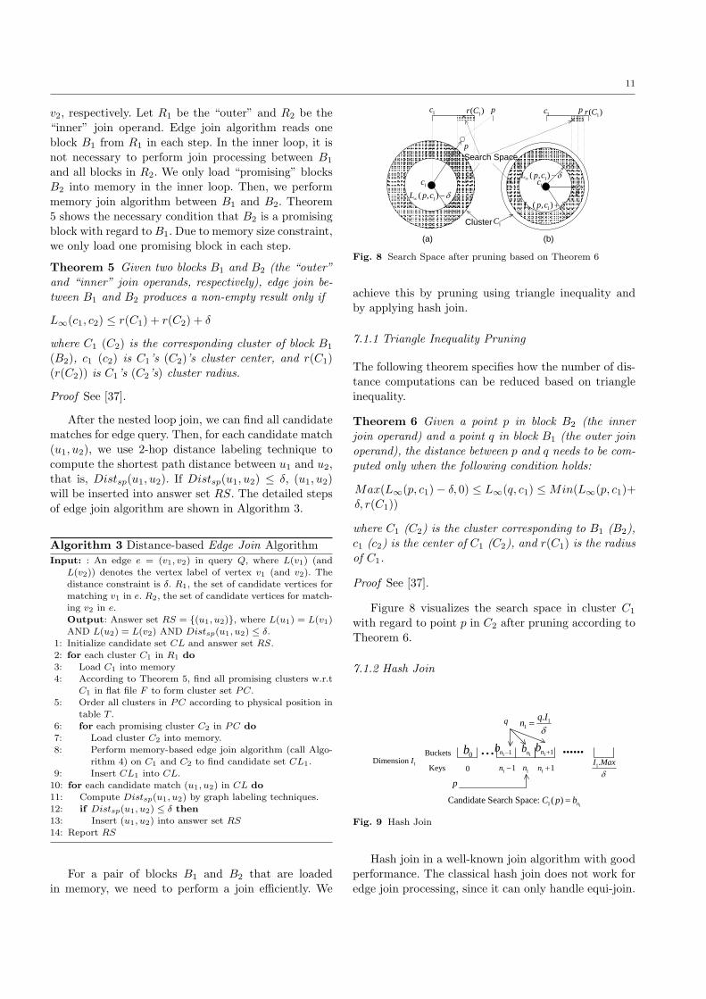
For a pair of blocks B1 and B2 that are loadedin memory, we need to perform a join efficiently. We
Search Space
(a) (b)
Cluster
1c 1( )r C p 1c p1( )r C
p
1C
1c1c
1( , )L p c δ∞ −
1( , )L p c δ∞ −
1( , )L p c δ∞ +
p
Fig. 8 Search Space after pruning based on Theorem 6
achieve this by pruning using triangle inequality andby applying hash join.
7.1.1 Triangle Inequality Pruning
The following theorem specifies how the number of dis-tance computations can be reduced based on triangleinequality.
Theorem 6 Given a point p in block B2 (the innerjoin operand) and a point q in block B1 (the outer joinoperand), the distance between p and q needs to be com-puted only when the following condition holds:
Max(L∞(p, c1)− δ, 0) ≤ L∞(q, c1) ≤ Min(L∞(p, c1)+δ, r(C1))
where C1 (C2) is the cluster corresponding to B1 (B2),c1 (c2) is the center of C1 (C2), and r(C1) is the radiusof C1.
Proof See [37].
Figure 8 visualizes the search space in cluster C1
with regard to point p in C2 after pruning according toTheorem 6.
7.1.2 Hash Join
... ......1
1.q Inδ
=q
1n1 1n − 1 1n +0
Buckets
Keys
0b 1 1nb − 1nb1 1nb +
1.I Maxδ
p
11Candidate Search Space: ( ) nC p b=
1Dimension I
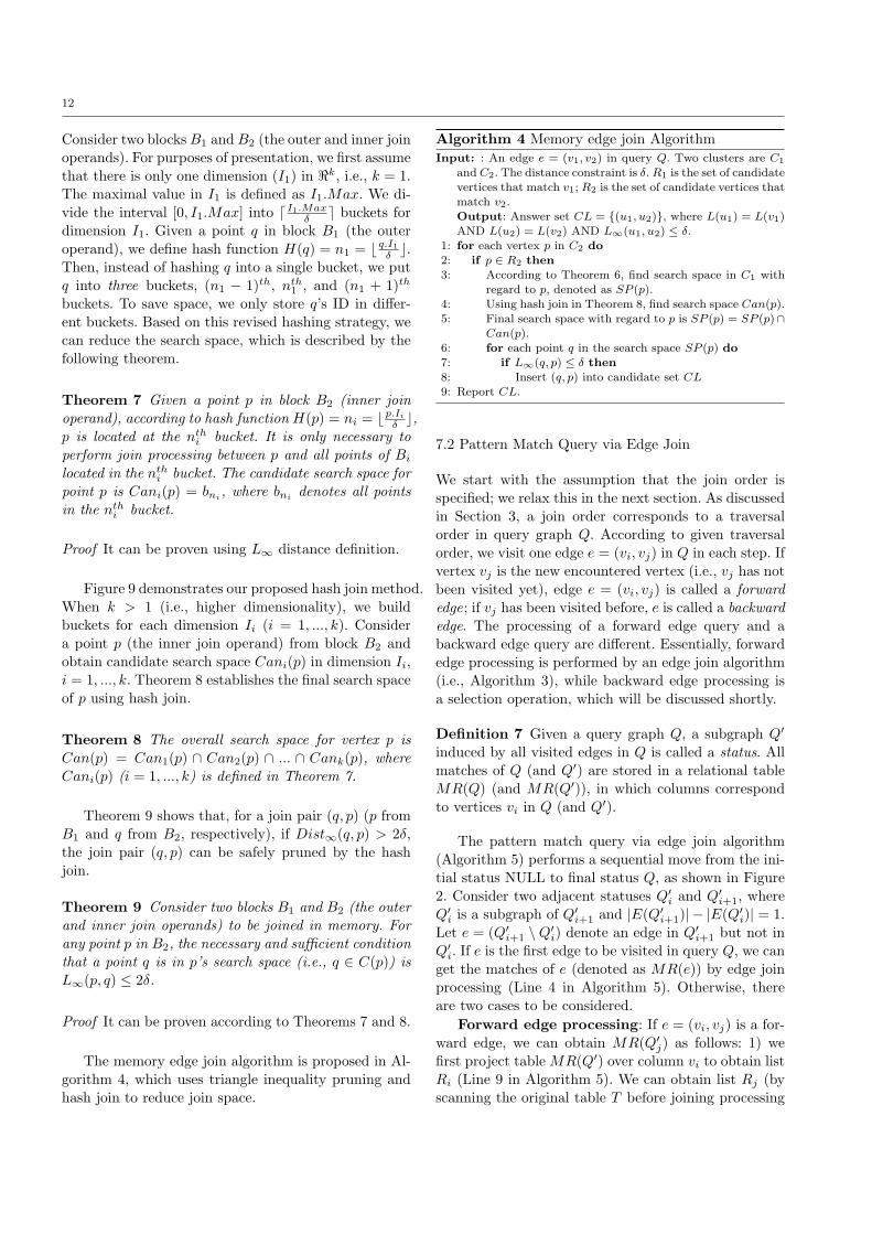
Fig. 9 Hash Join
Hash join in a well-known join algorithm with goodperformance. The classical hash join does not work foredge join processing, since it can only handle equi-join.
12
Consider two blocks B1 and B2 (the outer and inner joinoperands). For purposes of presentation, we first assumethat there is only one dimension (I1) in <k, i.e., k = 1.The maximal value in I1 is defined as I1.Max. We di-vide the interval [0, I1.Max] into d I1.Max
δ e buckets fordimension I1. Given a point q in block B1 (the outeroperand), we define hash function H(q) = n1 = b q.I1
δ c.Then, instead of hashing q into a single bucket, we putq into three buckets, (n1 − 1)th, nth
1 , and (n1 + 1)th
buckets. To save space, we only store q’s ID in differ-ent buckets. Based on this revised hashing strategy, wecan reduce the search space, which is described by thefollowing theorem.
Theorem 7 Given a point p in block B2 (inner joinoperand), according to hash function H(p) = ni = bp.Ii
δ c,p is located at the nth
i bucket. It is only necessary toperform join processing between p and all points of Bi
located in the nthi bucket. The candidate search space for
point p is Cani(p) = bni , where bni denotes all pointsin the nth
i bucket.
Proof It can be proven using L∞ distance definition.
Figure 9 demonstrates our proposed hash join method.When k > 1 (i.e., higher dimensionality), we buildbuckets for each dimension Ii (i = 1, ..., k). Considera point p (the inner join operand) from block B2 andobtain candidate search space Cani(p) in dimension Ii,i = 1, ..., k. Theorem 8 establishes the final search spaceof p using hash join.
Theorem 8 The overall search space for vertex p isCan(p) = Can1(p) ∩ Can2(p) ∩ ... ∩ Cank(p), whereCani(p) (i = 1, ..., k) is defined in Theorem 7.
Theorem 9 shows that, for a join pair (q, p) (p fromB1 and q from B2, respectively), if Dist∞(q, p) > 2δ,the join pair (q, p) can be safely pruned by the hashjoin.
Theorem 9 Consider two blocks B1 and B2 (the outerand inner join operands) to be joined in memory. Forany point p in B2, the necessary and sufficient conditionthat a point q is in p’s search space (i.e., q ∈ C(p)) isL∞(p, q) ≤ 2δ.
Proof It can be proven according to Theorems 7 and 8.
The memory edge join algorithm is proposed in Al-gorithm 4, which uses triangle inequality pruning andhash join to reduce join space.
Algorithm 4 Memory edge join AlgorithmInput: : An edge e = (v1, v2) in query Q. Two clusters are C1
and C2. The distance constraint is δ. R1 is the set of candidate
vertices that match v1; R2 is the set of candidate vertices thatmatch v2.
Output: Answer set CL = (u1, u2), where L(u1) = L(v1)
AND L(u2) = L(v2) AND L∞(u1, u2) ≤ δ.1: for each vertex p in C2 do
2: if p ∈ R2 then
3: According to Theorem 6, find search space in C1 withregard to p, denoted as SP (p).
4: Using hash join in Theorem 8, find search space Can(p).
5: Final search space with regard to p is SP (p) = SP (p)∩Can(p).
6: for each point q in the search space SP (p) do7: if L∞(q, p) ≤ δ then
8: Insert (q, p) into candidate set CL
9: Report CL.
7.2 Pattern Match Query via Edge Join
We start with the assumption that the join order isspecified; we relax this in the next section. As discussedin Section 3, a join order corresponds to a traversalorder in query graph Q. According to given traversalorder, we visit one edge e = (vi, vj) in Q in each step. Ifvertex vj is the new encountered vertex (i.e., vj has notbeen visited yet), edge e = (vi, vj) is called a forwardedge; if vj has been visited before, e is called a backwardedge. The processing of a forward edge query and abackward edge query are different. Essentially, forwardedge processing is performed by an edge join algorithm(i.e., Algorithm 3), while backward edge processing isa selection operation, which will be discussed shortly.
Definition 7 Given a query graph Q, a subgraph Q′
induced by all visited edges in Q is called a status. Allmatches of Q (and Q′) are stored in a relational tableMR(Q) (and MR(Q′)), in which columns correspondto vertices vi in Q (and Q′).
The pattern match query via edge join algorithm(Algorithm 5) performs a sequential move from the ini-tial status NULL to final status Q, as shown in Figure2. Consider two adjacent statuses Q′
i and Q′i+1, where
Q′i is a subgraph of Q′
i+1 and |E(Q′i+1)| − |E(Q′
i)| = 1.Let e = (Q′
i+1 \Q′i) denote an edge in Q′
i+1 but not inQ′
i. If e is the first edge to be visited in query Q, we canget the matches of e (denoted as MR(e)) by edge joinprocessing (Line 4 in Algorithm 5). Otherwise, thereare two cases to be considered.
Forward edge processing: If e = (vi, vj) is a for-ward edge, we can obtain MR(Q′
j) as follows: 1) wefirst project table MR(Q′) over column vi to obtain listRi (Line 9 in Algorithm 5). We can obtain list Rj (byscanning the original table T before joining processing
13
in Line 1) that corresponds to vertex vj , according tovj ’s label. Note that, Rj is a shrunk list after neighborarea pruning (Line 2); 2) According to the edge joinalgorithm (Algorithm 3), we find the matches for edgee, denoted as MR(e) (Line 10); 3) We perform tradi-tional natural join over MR(Q′
i) and MR(e) to obtainMR(Q′
j) based on column vi (Line 11).Backward edge processing: If e = (vi, vj) is a
backward edge, we scan the intermediate table MR(Q′i)
to filter out all vertex pairs (ui, uj), where ui and uj cor-respond to vertices vi and vj in query Q, and Distsp(ui, uj)> δ. After filtering MR(Q′
i), we obtain the matches ofQ′
i+1, i.e., MR(Q′i+1). Essentially, it is a selection oper-
ation based on the distance constraint (Line 13), definedas follows: MR(Q′
i+1) = σ(Distsp(r.vi,r.vj)≤δ)(MR(Q′i)).
The above steps are iterated until the final status Qis reached (Lines 6-13).
7.3 Cost Model
It is well-known that each join order in Algorithm 5will lead to a different performance. The join order se-lection is based on the cost estimation of edge query.The cost of edge join algorithm has three components:the cost of block nested loop join (Lines 2-10 in Algo-rithm 3), the cost of computing the exact shortest pathdistance (Lines 12-14), and the cost of storing answerset RS (Line 15). Note that the matches of an edgequery are intermediate results for graph pattern query.Therefore, similar to cost analysis for structural joinin XML databases [32], we also assume that interme-diate results are stored in a temporary table on disk.We use a set of factors to normalize the cost of edgejoin algorithm. These factors are fR: the average costof loading one block into memory; fD: the average costof L∞ distance computation; fS : the average cost ofshortest path distance computation; and fIO: the aver-age cost of storing one match on disk. Given an edgequery Qe = (v1, v2) and a parameter δ, R1 (R2) is thelist of candidate vertices for matching v1 (v2). All ver-tices in R1 (R2) are stored in |B1| (|B2|) blocks in aflat file F . The cost of Algorithm 3 can be computed asfollows:
Cost(e) =|B1| × |B2| × γ1 × fR + |R1| × |R2| × γ2 × fD+|CL| × fS + |CL| × γ3 × fIO
(7)
where γ1, γ2, and γ3 are defined as follows.
γ1 =|AccessedBlocks|
|B1| × |B2|, γ2 =
|DisComp||R1| × |R2|
, γ3 =|RS||CL|
(8)
and where |AccessedBlocks| is the number of accessedblocks in Algorithm 3; |DisComp| is the number of L∞distance computations and |RS| (and |CL|) is the car-dinality of answer set RS (and candidate set CL). Weuse the following methods to estimate γ1, γ2 and γ3.
1) Offline: We pre-compute γ1, γ2 and γ3. Noticethat γ1, γ2 and γ3 are related to vertex labels and thedistance constraint δ. Thus, according to historical querylogs, the maximal value of δ is δ. We partition [0, δ] intoz intervals, each with width d = d δ
z e. In order to com-pute the statistics γ1, γ2 and γ3 for vertex label pair(l1, l2) and the distance constraint δ in the ith interval[(i − 1)d, i ∗ d] (1 ≤ i ≤ z), we set δ = (i − 1/2)d, andthere is only one edge e = (v1, v2) in query graph Qwhere L(v1) = l1 and L(v2) = l2. We perform edge joinand compute γ1, γ2 and γ3 using Equation 8.
2) Online: Given an edge query Qe = (v1, v2), welook up the estimates for γ1, γ2 and γ3 that were com-puted offline using the vertex label (L(v1), L(v2)) andδ.
Algorithm 5 Multiway Distance-Join Algorithm (MD-Join)Input: Input: A query graph Q that has n vertices and a pa-
rameter δ and a large graph G and a table T for the converted
vector space <k, and the join order MDJ .
Output: MR(Q): All matches of Q in G.1: for each vertex vi in query Q, find its corresponding list Ri,
according to vi’s label.
2: Obtain Shrunk lists Ri (i = 1, ..., n) by neighbor area prun-ing.
3: Set e = (v1, v2).
4: Obtain MR(e) by edge join algorithm (call Algorithm 3).5: set Q′i = e.
6: while Q′i! = Q do7: According to join order MDJ , e is the next traversal edge.
8: if e is forward edge, denoted as e = (vi, vj) then
9: Ri = σt.ID∈(∏
viMR(Q′
i))(T ) .
10: MR(e) =∏
(Ri.ID,Rj .ID) ( Ri ./ RjDistsp(ri,rj)≤δ
) (call
Algorithm 3)11: MR(Q′
i+1) = MR(Q′i) ./ MR(e)
vi
12: else13: MR(Q′i+1) = σ(Distsp(r.vi,r.vj)≤δ)(MR(Q′i))14: Report MR(Q).
Given an edge query Qe = (v1, v2), the cardinal-ity of candidate match set CL can be computed as|CL| = |R1| × |R2| × θ where θ is the selectivity of D-join based on L∞ distance. Therefore, the key issue ishow to estimate θ. We propose two methods, one basedon probability-model and the other on sampling.
14
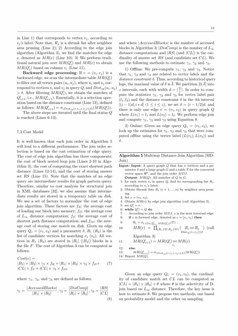
7.4 Probability Model For Estimating θ
Given an edge query Qe = (v1, v2), according to vertexlabel, we can find two vertex lists R1 and R2. For thepurposes of presentation, let us first assume that k = 1,i.e., there is one dimension in the converted space. Wecan regard R1.I1 and R2.I1 as two random variables xand y. Let z = |x−y| denote the joint random variable.Selectivity θ equals to the probability of z ≤ δ. Figure10(a) visualizes the joint random variable z and thearea Ω between two curves y = x + δ and y = x − δ.We can compute selectivity θ as follows:
θ = Pr(z ≤ δ) =∫ ∫
|x−y|≤δ
f(x, y)d(x, y) =∫ ∫(x,y)∈Ω
f(x, y)d(x, y)
where f(x, y) denotes z’s density function. We use two-dimensional histogram method to estimate f(x, y). Specif-ically, we use equi-width histograms that partition (x, y)data space into t2 regular buckets (where t is a constantcalled the histogram resolution), as shown in Figure10(b). Similar to other histogram methods, we also as-sume that the distribution in each bucket is uniform.Then, we use a systematic sampling technique [14] toestimate the density function in each bucket.
The basic idea of systematic sampling is the fol-lowing: Given a relation R with N tuples that can beaccessed in ascending/descending order on the join at-tribute of R, we select n sample tuples as follows: selecta tuple at random from the first dN
n e tuples of R andevery dN
n eth tuple thereafter [14]. The relations hereare R1 and R2, and the join attributes are R1.I1 andR2.I1, where R1 and R2 are both from table T . Weassume that there exists a B+-tree index on each di-mension Ii in table T , allowing tuples to be accessed inascending/descending order. We select |R1|×λ verticesfrom R1, and all these selected vertices are collected toform subset SR1, where λ is a sampling ratio. The sameis done for subset SR2 from the list R2.
δ
δ
2 1 1 1. .R I R I δ= +
2 1 1 1. .R I R I δ= −
1 1.R I
2 1.R I
The Shade Area Ω
(a)
δ
δ1
1
2
32
12f
11f 21f 31f
32f
33f23f13f
2 1 1 1. .R I R I δ= +
2 1 1 1. .R I R I δ= −
1 1.R I
2 1.R IThe Shade Area Ω
22f
(b)
Fig. 10 Selectivity Estimation
We map SR1 × SR2 into different two-dimensionalbuckets. For each bucket A, we use |A| to denote thenumber of points (from SR1×SR2) that fall into bucketA. The joint density function of points in bucket A isdenoted as
f(A) =|A|
|SR1| × |SR2|. (9)
Some buckets are partially contained in the sharedarea Ω. The number of points (from R1 ×R2) that fallinto both bucket A and the shared area Ω (denoted as|A ∩Ω|) can be estimated as:
|A ∩Ω| = R1 ×R1 × f(A)× area(A ∩Ω)area(A)
where area(A∩Ω) denotes the area of intersection be-tween A and Ω and area(A) denotes the area of A.
We adopt Monte-Carlo methods to estimate area(A∩Ω)area(A) .
Specifically, we first randomly generate a set of pointsin bucket A (the number of generated records is a). Thenumber of points that fall in Ω is b. Then, we estimatearea(A∩Ω)
area(A) to be ab .
Therefore, we have |CL| =∑
ij |Aij ∩Ω| = |R1| ×|R2| ×
∑ij (f(Aij)× area(Aij∩Ω)
area(Aij))
The selectivity of θ can be estimated as follows
θ = Pr(z ≤ δ) =∑
ij |Aij ∩Ω| =∑ij (f(Aij)× area(Aij∩Ω)
area(Aij))
(10)
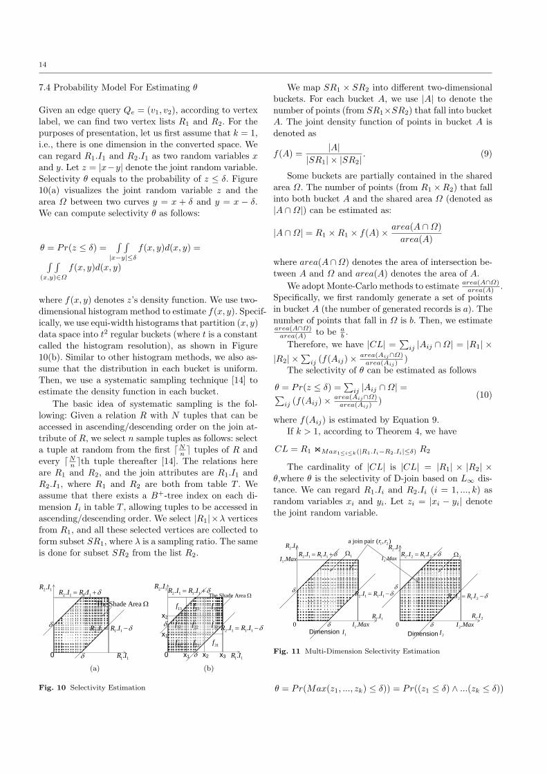
where f(Aij) is estimated by Equation 9.If k > 1, according to Theorem 4, we have
CL = R1 onMax1≤i≤k(|R1.Ii−R2.Ii|≤δ) R2
The cardinality of |CL| is |CL| = |R1| × |R2| ×θ,where θ is the selectivity of D-join based on L∞ dis-tance. We can regard R1.Ii and R2.Ii (i = 1, ..., k) asrandom variables xi and yi. Let zi = |xi − yi| denotethe joint random variable.
δ
δ 1.I Max
1.I Max
0
δ
δ 2.I Max
2.I Max
0
2 2 1 2. .R I R I δ= +2 1 1 1. .R I R I δ= +
2 1 1 1. .R I R I δ= −2 2 1 2. .R I R I δ= −
2 2.R I1Ω
2Ω
1 2a join pair ( , )r r
Dimension 1I Dimension 2I
1 2.R I
2 1.R I
1 1.R I
Fig. 11 Multi-Dimension Selectivity Estimation
θ = Pr(Max(z1, ..., zk) ≤ δ)) = Pr((z1 ≤ δ) ∧ ...(zk ≤ δ))
15
(11)
In order to compute Equation 11, we assume thatevery dimension Ii in vector space <k is independent ofeach other. Thus, we have
Pr((z1 ≤ δ)∧...∧(zk ≤ δ)) = Pr(z1 ≤ δ)×...×Pr(zk ≤ δ).
(12)
where Pr(zi ≤ δ) (i = 1, ..., k) can be computed usingEquation 11.
7.5 Sampling-based Method
Consider two lists R1 and R2 to be joined. Assume, forsimplicity, k = 2. In Figure 11, Pr(Max(z1, z2) ≤ δ)) isthe probability that a vertex pair falls into both sharedareas Ω1 and Ω2. We adopt sampling-based methodsto estimate Pr(Max(z1, ..., zk) ≤ δ)). For example, wehave two sample sets SR1 and SR2 from two sets R1
and R2, respectively. If there are M join pairs (u1, u2)such that Max(|u1.Ii−u2.Ii|) ≤ δ, (1 ≤ i ≤ k), Pr(Max(z1, ..., zk) ≤ δ) = M
|SR1|×|SR2| . The specific techniquefor computing the optimal sampling technique in high-dimensional space is beyond the scope of this paper.Without loss of generality, we choose random samples,i.e., each point has equal probability of being chosen asa sample.
7.6 Join Order Selection
The join order selection can be performed by adoptingthe traditional dynamic programming algorithm [32]using the cost model introduced in the previous section.However, this solution is inefficient due to the very largesolution space, especially when |E(Q)| is large. There-fore, we propose a simple yet efficient greedy solutionto find a good join order. As mentioned earlier, one joinorder corresponds to one traversal order in query graphQ, according to which, one edge (of Q) is visited in eachstep. In each step, the subgraph Q′ that is formed bycollecting all edges that have been visited is called astatus (Definition 7). Obviously, status Q′ moves fromNULL to Q according to the specified join order. Thereare two important heuristic rules in our join order se-lection.
1) Given a status Q′i, if there is a backward edge e
attached to Q′i, the next status is Q′
i+1 = Q′i ∪ e, i.e.,
we perform back edge processing as early as possible.If there are more than one backward edges attached toQ′
i, we perform all back edge processing simultaneously,which will reduce the I/O cost.
The intuition behind this heuristic rule is similar to“selection push-down” in relational query optimization.Performing back edge query will reduce the cardinalityof intermediate join results.
2) Given a status Q′i, if there is no backward edge
attached to Q′i, the next status is Q′
i+1 = Q′i ∪ e, where
e is a forward edge and Cost(e) (defined in Equation 7)is minimum of all forward edges.
8 Bi-Level Distance Join
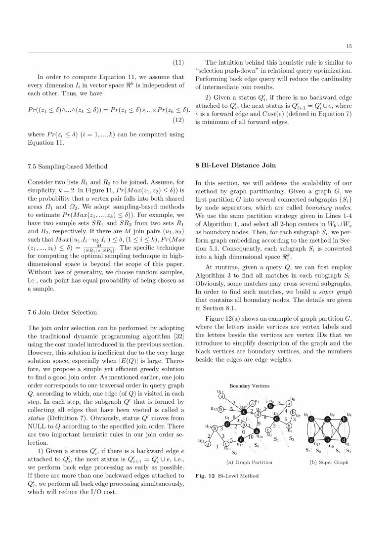
In this section, we will address the scalability of ourmethod by graph partitioning. Given a graph G, wefirst partition G into several connected subgraphs Siby node separators, which are called boundary nodes.We use the same partition strategy given in Lines 1-4of Algorithm 1, and select all 2-hop centers in Wb ∪Ws
as boundary nodes. Then, for each subgraph Si, we per-form graph embedding according to the method in Sec-tion 5.1. Consequently, each subgraph Si is convertedinto a high dimensional space <k
i .
At runtime, given a query Q, we can first employAlgorithm 3 to find all matches in each subgraph Si.Obviously, some matches may cross several subgraphs.In order to find such matches, we build a super graphthat contains all boundary nodes. The details are givenin Section 8.1.
Figure 12(a) shows an example of graph partition G,where the letters inside vertices are vertex labels andthe letters beside the vertices are vertex IDs that weintroduce to simplify description of the graph and theblack vertices are boundary vertices, and the numbersbeside the edges are edge weights.
c
a
da
ab
dbd
b
b
a
c
Boundary Vertices
b
ca S0
S1
S2
S3u3
u8
u9
d
a
u10
u11
u12
u1
3u14
u15
u16u17
u2
u4u1
u5
u6
u7u18
35 7
2 18
9
345 3
11
21
8
3
532
1
10
3
(a) Graph Partition
cd
ad
b
d
u1
u17 u10
u9
u5
u4
S2 S0 S1 S3
(b) Super Graph
Fig. 12 Bi-Level Method
16
8.1 Offline Processing
Algorithm 6 depicts the whole offline processing frame-work. First, we partition G into some subgraphs Si(Line 1 in Algorithm 6). Then, for each subgraph Si,we employ graph embedding to convert Si into a multi-dimensional space <k
i (Line 3). According to the methodin Algorithm 1, we can compute 2-hop labeling for eachsubgraph Si (Line 4). In order to address the matchesthat cross several subgraphs, we build a super graphGs, that will be discussed shortly. We also employ graphembedding to convert Gs into the converted space <k
super,and compute the 2-hop labeling for Gs (Lines 6-7).
We employ the method in [4] to construct a su-per graph Gs. Specifically, a super graph consists of allboundary nodes as vertices and two vertices are con-nected by an edge directly when they are in the samesubgraph Si. The edge in a super graph is called a superedge whose weight is the shortest path distance betweentwo vertices in the subgraph involved. Given the graphpartition in Figure 12(a), Figure 12(b) shows the corre-sponding super graph Gs, which contains all bound-ary nodes. In each subgraph Si, we introduce superedges between all pairwise boundary nodes, where theedge weight denotes the corresponding pairwise short-est path distance in Si. For example, since vertices u9
and u10 are boundary vertices in segment S0, we in-troduce an edge e1 = (u9, u10) in Gs, whose weightis the shortest path distance between u9 and u10 insubgraph S0. Note that, u9 and u10 are also boundarynodes in subgraph S2, thus, we introduce another edgee2 = (u9, u10) in Gs, whose weight denotes the short-est path distance between u9 and u10 in subgraph S2.Therefore, there are two edges with different weightsbetween u9 and u10 in Gs, meaning that Gs is a multi-graph. Actually, if there is more than one edge betweentwo vertices, we can keep only the edge (u9, u10) withthe minimal weight and remove others by postprocess-ing. Therefore, in the following discussion, we can stillassume that Gs is a graph, not a multigraph. Then, wealso utilize graph embedding technique to convert Gs
into a multi-dimensional space <ksuper.
In summary, at the end of offline processing, wehave the following pre-computed results: 1) For eachsubgraph Si, there is a table Ti that stores all multi-dimensional points in the converted space <k
i ; 2) Thereis a table Tsuper to store all multi-dimensional pointsthat in the converted space <k
super; 3) For each sub-graph Si and the super graph Gs, there is also a tableto store 2-hop labels for Si and Gs.
Algorithm 6 Offline Processing in Bi-Level MethodInput: Input:Graph G.
Output: Ti(Tsuper): the converted multi-dimensional space
for each subgraph Si and Gs; 2HopLabel(Si) and2HopLabel(Gs): the 2-hop labeling for each subgraph Si and
Gs.
1: Partition G into m subgraphs S1, ..., Sm.2: for each subgraph Si do
3: Employ graph embedding to map Si into the converted
space Ti.4: Employ Algorithm 1 to compute 2-hop labeling for Si,
denoted as 2HopLabel(Si).
5: Build the super graph Gs.6: Employ graph embedding to map Gs into the converted space
Tsuper.
7: Employ Algorithm 1 to compute 2-hop labeling for Gs, de-noted as 2HopLabel(Gs).
cd
ad
u1
u17 u10
u9cd
ad
u13
u10
u9
a u18
(a) (b)
32
22
32
1
1
1
u17
Fig. 13 Optimization For Super Graph Construction
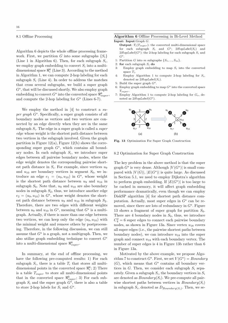
8.2 Optimization for Super Graph Construction
The key problem in the above method is that the supergraph Gs is very dense. Although |V (Gs)| is small com-pared with |V (G)|, |E(Gs)| is quite large. As discussedin Section 5.1, we need to employ Dijkstra’s algorithmto perform graph embedding. If |E(Gs)| is too large tobe cached in memory, it will affect graph embeddingperformance dramatically, even though we can employDiskSP algorithm [4] for shortest path distance com-putation. Actually, most super edges in Gs can be re-moved, since there are lots of redundancy in Gs. Figure13 shows a fragment of super graph for partition S0.There are 4 boundary nodes in S0, thus, we introduceC2
4 = 6 super edges to connect each pairwise boundarynodes, as shown in Figure 13a. Since vertex u18 coversall super edges (i.e., the pairwise shortest paths betweenboundary nodes), we can introduce u18 into the supergraph and connect u18 with each boundary vertex. Thenumber of super edges is 4 in Figure 13b rather than 6in Figure 13a.
Motivated by the above example, we propose Algo-rithm 7 to construct Gs. First, we set V (Gs) = Boundary(G), which means that Gs contains all boundary ver-tices in G. Then, we consider each subgraph Si sepa-rately. Given a subgraph Si, the boundary vertices in Si
are denoted as Boundary(Si). We pre-compute all pair-wise shortest paths between vertices in Boundary(Si)in subgraph Si, denoted as DBoundary(Si). Then, we se-

17
lect a vertex u (in Si) to maximize |DBoundary(Si,u)|,where DBoundary(Si,u) denotes all paths in DBoundary(Si)
that pass through u. We introduce edges between uand each path endpoint in DBoundary(Si,u). We removeDBoundary(Si,u) from DBoundary(Si). The above processis iterated until |DBoundary(Si)| < 2×|DBoundary(Si,u)|.The intuition behind the stop condition is as follows.Assume that one vertex u is selected to maximize |DBoundary(Si,u)| in some iteration step. We need to intro-duce extra 2× |DBoundary(Si,u)| edges to connect u andpath endpoints DBoundary(Si,u) in Gs. If |DBoundary(Si)|< 2×|DBoundary(Si,u)|, it means that the number of theuncovered pairwise shortest paths is less than the num-ber of introduced extra edges. Thus, we can introducean edge between two path endpoints in DBoundary(Si)
directly, and the edge weight is the corresponding short-est path distance. Finally, if there are multi-edges be-tween two vertices in Gs, we only keep one edge withthe minimal weight.
Algorithm 7 Optimization For Subgraph Graph Con-structionInput: Input: Boundary(G): the boundary vertices in G; Si:
each subgraph in G.Output: The subgraph G′.
1: set V (G′) = Boundary(G).
2: for each subgraph Si do3: Set DBoundary(Si)
= u1u2|u1, u2 ∈ Boundary(Si),where u1u2 denotes the shortest path between u1 and u2.
4: repeat5: Select a vertex u in Si to maximize |DBoundary(Si,u)|,
where DBoundary(Si,u) = u1u2|(u1, u2 ∈Boundary(Si)) ∧ (u ∈ u1u2).
6: Introduce edges between u and endpoints in
DBoundary(Si,u).7: DBoundary(Si)
= DBoundary(Si)−DBoundary(Si,u).
8: Introduce an edge between u1 and u2, where u1u2 ∈DBoundary(Si)
.9: until |DBoundary(Si)
| < 2× |DBoundary(Si,u)|10: for each vertex pair (u1, u2), where u1, u2 ∈ Boundary(G)
do11: if there are multi edges between u1 and u2 then
12: Only keep the edge with the minimal weight.
8.3 Online Processing
At run time, given a query graph Q, we also employthe framework described in Section 3 to find matchesof Q, i.e., answering Q by a series of edge queries. Con-sequently, the key problem in answering Q is how toanswer the edge query efficiently. To distinguish fromthe method in Section 7, we call the following algorithmbi-level distance join (bD-join for short) algorithm.
Algorithm 9 shows a nested-loop join algorithm toanswer edge query. In each loop, we join vertices from
Algorithm 8 bD-Join AlgorithmInput: Input: an edge query e = (v0, v1) and a parameter δ and
two subgraph S1 and S2.
Output: Answer set RS(S1, S2).1: According to vertex labels, we find two vertex lists R1 (from
S1) and R2 (from S2) that corresponds to v1 and v2, respec-
tively.2: Employ Algorithm 3 to find RS1α1 = R1 ./ Boundary(P1)
Distsp(u1,u2)≤δ
,
where Boundary(P1) denotes all boundary vertices in P1.
3: Employ Algorithm 3 to find RSα22 = Boundary(P2) ./ R2Distsp(u1,u2)≤δ
.
4: Employ Algorithm 3 to find RSα1α2 =
Boundary(S1) ./ Boundary(S2)Distsp(u1,u2)≤δ
.
5: RS(S1, S2) = σ(RS1α1 .dist+RSα1a2 .dist+RSα22.dist≤δ)(RS1α1./
RSα1α2 ./ RSα22).
6: Return RS(S1, S2).
Boundary Vertices
Shortest Distance Path
u1
u2
Shortest Distance Path
u1
u2
u1
u2
Boundary Vertices
Shortest Distance
Path
P1
P2
P1 , P2
P1 , P2
(a) (b) (c)
Fig. 14 Shortest Distance Path
S1 and S2. Specifically, according to vertex labels, wecan find two vertex lists R1 (from S1) and R2 (fromS2) that correspond to v1 and v2, respectively. Thereare two cases namely, S1 6= S2 and S1 = S2.
1) S1 6= S2: We first propose how to join R1 (fromS1) and R2 (from S2) in Algorithm 8, where S1 6= S2.Considering two vertices u1 and u2 in S1 and S2, re-spectively, the shortest path between u1 and u2 mustgo through a boundary vertex in Boundary(S1) and aboundary vertex in Boundary(S2). Based on distanceconstraint δ, we can employ Algorithm 3 to join R1 andBoundary(S1) to obtain RS1α1 = R1 onDistsp(u1,u2)≤δ
Boundary(S1) (Line 2 in Algorithm 8). We also joinBoundary(S2) and R2 to obtain RSα22, where RSα22 =Boundary(S2) onDistsp(u1,u2)≤δ R2 (Line 3). In the su-per graph Gs, we also employ Algorithm 3 to join Boundary(S1) and Boundary(S2), i.e., RSα1α2 = Boundary(S1)onDistsp(u1,u2)≤δ Boundary(S2) (Line 3). The three tem-porary table formats (RS1α1 , RSα1α2 and RSα22) areshown in Figure 15. Finally, we perform natural joinsbetween three tables to obtain final matches for edgequery e = (v1, v2) by the following SQL query (Line 5).Select Distinct(RS1α1 .u1, RSα22.u2)
From RS1α1 ,RSα22, RS2α2
Where RS1α1 .α1 = RSα1α2 .α1
AND RSα1α2 .α2 = RS2α2 .α2 AND (RS1α1 .dist+
RSα1α2 .dist + RSα22.dist <= δ)
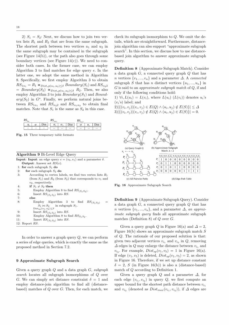
18
2) S1 = S2: Next, we discuss how to join two ver-tex lists R1 and R2 that are from the same subgraph.The shortest path between two vertices u1 and u2 inthe same subgraph may be contained in the subgraph(see Figure 14(b)), or the path also goes through someboundary vertices (see Figure 14(c)). We need to con-sider both cases. In the former case, we can employAlgorithm 3 to find matches for edge query e. In thelatter one, we adopt the same method in Algorithm8. Specifically, we first employ Algorithm 3 to obtainRS1α1 = R1 onDistsp(u1,u2)≤δ Boundary(S1) and RSα22
= Boundary(S2) onDistsp(u1,u2)≤δ R2. Then, we alsoemploy Algorithm 3 to join Boundary(S1) and Bound-ary(S2) in Gs. Finally, we perform natural joins be-tween RS1α1 and RSα22 and RSα1α2 to obtain finalmatches. Note that S1 is the same as S2 in this case.
Dist… … …
11RS α
α Dist… … …
α2 2RSα
Dist… … …
1α1 2
RSα α
2α1u 2u
Fig. 15 Three temporary table formats
Algorithm 9 Bi-Level Edge QueryInput: Input: an edge query e = (v0, v1) and a parameter δ.
Output: Answer set RS(e).1: for each subgraph S1 do
2: for each subgraph S2 do
3: According to vertex labels, we find two vertex lists R1
(from S1) and R2 (from S2) that corresponds to v1 and
v2, respectively.4: if S1 6= S2 then
5: Employ Algorithm 8 to find RS(S1S2).
6: Insert RS(S1S2) into RS.7: else
8: Employ Algorithm 3 to find RS(S1S2) =
S1 ./ S2Distsp(u1,u2)≤δ
in subgraph S1.
9: Insert RS(S1S2) into RS.10: Employ Algorithm 8 to find RSS1S2 .
11: Insert RS(S1S2) into RS.
12: Report RS.
In order to answer a graph query Q, we can performa series of edge queries, which is exactly the same as theproposed method in Section 7.2.
9 Approximate Subgraph Search
Given a query graph Q and a data graph G, subgraphsearch locates all subgraph isomorphisms of Q overG. We can simply set distance constraint δ = 1 andemploy distance-join algorithm to find all (distance-based) matches of Q over G. Then, for each match, we
check its subgraph isomorphism to Q. We omit the de-tails, which are straightforward. Furthermore, distance-join algorithm can also support “approximate subgraphsearch”. In this section, we discuss how to use distance-based join algorithm to answer approximate subgraphquery.
Definition 8 (Approximate Subgraph Match). Considera data graph G, a connected query graph Q that hasn vertices v1, ..., vn and a parameter ∆. A connectedsubgraph S that has n distinct vertices u1, ..., un inG is said to an approximate subgraph match of Q, if andonly if the following conditions hold:1) ∀i, L(ui) = L(vi), where L(ui) (L(vi)) denotes ui’s(vi’s) label; and2)|(vi, vj)|(vi, vj) ∈ E(Q) ∧ (ui, uj) /∈ E(S)| ≤ ∆3)|(vi, vj)|(vi, vj) /∈ E(Q) ∧ (ui, uj) ∈ E(S)| = 0.
1v
2v3v
4v
5v
6v
7v
1v 5v1v 5v
1v 7v 5v
1v 7v 6v5v
1v 2v 3v 4v5v
1 5v v 1 7v v 7 5v v 7 6v v 6 5v v1P
2P
3P
1P
2P
3P
4P(c) All Pairwise Paths (d) Edge-Path Table
(a) Query Graph Q
1u
2u3u
4u
5u
6u
7u
(b) Approximate Subgraph Match 2Δ =
1 2v v 2 3v v 3 4v v 4 5v v
4P
Fig. 16 Approximate Subgraph Search
Definition 9 (Approximate Subgraph Query). Considera data graph G, a connected query graph Q that hasn vertices v1, ..., vn, and a parameter ∆, an approx-imate subgraph query finds all approximate subgraphmatches (Definition 8) of Q over G.
Given a query graph Q in Figure 16(a) and ∆ = 2,Figure 16(b) shows an approximate subgraph match Sof Q. The rationale of our proposed solution is that:given two adjacent vertices vi1 and vi2 in Q, removing∆ edges in Q may enlarge the distance between vi1 andvi2 . For example, Distsp(v1, v5) = 1 in Figure 16(a).If edge (v1, v5) is deleted, Distsp(v1, v5) = 2, as shownin Figure 16. Therefore, if we set up distance constantδ = 2, S (in Figure 16(b)) is also a (distance-based)match of Q according to Definition 1.
Given a query graph Q and a parameter ∆, foreach edge (vi1 , vi2) in query Q, we first compute anupper bound for the shortest path distance between vi1
and vi2 (denoted as Distmax(vi1 , vi2)), if ∆ edges are
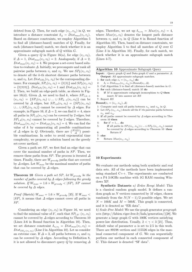
19
deleted from Q. Then, for each edge (vi1 , vi2) in Q, weintroduce a distance constraint δij = Distmax(vi, vj).Based on distance constraints, we employ Algorithm 5to find all (distance-based) matches of Q. Finally, foreach (distance-based) match, we check whether it is anapproximate subgraph match of Q within G.
Given a query Q in Figure 16(a), for edge (v1, v5),if ∆ = 1, Distmax(v1, v5) = 2. Analogously, if ∆ = 2,Distmax(v1, v5) = 4. We propose a set-cover based solu-tion to evaluate ∆. Initially, we precompute and rank allpairwise paths between v1 and v5. We use SPk(v1, v5)to denote all the k-th shortest distance paths betweenv1 and v5. Let DistSPk
(v1, v2) be the corresponding dis-tance. For example, SP1(v1, v5) = v1v5 and SP2(v1, v5)= v1v7v5. DistSP1(v1, v5) = 1 and DistSP2(v1, v5) =2. Then, we build an edge-path table, as shown in Fig-ure 16(d). Given ∆, we need to find k, where SP1,k−1
(v1, v5) = SP1(v1, v5) ∪ ... ∪ SPk−1(v1, v5) can becovered by ∆ edges, but SP1,k(v1, v5) = SP1(v1, v5)∪... ∪ SPk(v1, v5) cannot be covered by ∆ edges. Forexample, in Figure 16, if ∆ = 2, we can find k = 4, sinceall paths in SP1,3(v1, v5) can be covered by 2 edges, butSP1,4(v1, v5) cannot be covered by 2 edges. Therefore,Distmax(v1, v5) = DistSP4(v1, v5) = 4. We can find thevalue of k by enumerating all possible combinationsof ∆ edges in Q. Obviously, there are
(|E(Q)|∆
)possi-
ble combinations. In order to avoid exponential timecomplexity, we propose a solution based on the greedyset-cover method.
Given a path set SP , we first find an edge that cancover the maximal number of paths in SP . Then, weremove these paths from SP . The process is iterated ∆times. Finally, there are Wgreedy paths that are coveredby ∆ edges. Let Wmax be the maximal number of pathsthat can be covered by ∆ edges.
Theorem 10 Given a path set SP , let Wgreedy be thenumber of paths covered by ∆ edges following the greedysolution. If Wmax = 1.6 × Wgreedy < |SP |, SP cannotbe covered by ∆ edges.
Proof (Sketch) Wmax = 1.6×Wgreedy [35]. If Wmax <|SP |, it means that ∆ edges cannot cover all paths inSP .
Considering an edge (v1, v5) in Figure 16, we needto find the minimal value of k′, such that SP1,k′ (v1, v5)cannot be covered by ∆ edges according to Theorem 10(Lines 3-6 in Bound function in Algorithm 10). Then,we set distance constraint δv1v5 = Distmax(v1, v5) =DistSPk′ (v1,v5) (Line 2 in Algorithm 10). Let us consideran extreme case. If ∆ = 3, all paths between v1 and v5
can be covered by ∆ edges. According to Definition 8,it is not allowed to disconnect query Q by removing ∆
edges. Therefore, we set up δv1v5 = Max(v1, v5) = 4,where Max(v1, v5) denotes the longest path distancebetween v1 and v5 in Q (Line 8 in Bound function ofAlgorithm 10). Then, based on distance constraints, weemploy Algorithm 5 to find all matches of Q over G(Line 3 in Algorithm 10). Finally, for each match, wecheck whether it is an approximate subgraph match(Lines 4-7).
Algorithm 10 Approximate Subgraph QueryInput: : Query graph Q and Data graph G and a parameter ∆.
Output: All approximate subgraph matches.
1: for each edge ei = (vi1 , vi2 ) do
2: δi = Distmax(vi1 , vi2 )=Bound(ei, ∆).3: Call Algorithm 5 to find all (distance-based) matches in G.
4: for each (distance-based) match M do
5: if M is approximate subgraph isomorphism to Q then6: insert M into answer set RS
7: Report RS
Bound(ei = (vi1 , vi2 ), ∆)
1: Compute and rank all paths between vi1 and vi2 in Q.2: Let SPk′ (vi1 , vi2 ) denote all the k′-th pairwise paths between
vi1 and vi2 .
3: if all paths cannot be covered by ∆ edges according to The-orem 10 then
4: for k′ = 1, ... do5: if all paths in SP1(vi1 , vi2 )∪ ...∪SPk′ (vi1 , vi2 ) cannot
be covered by ∆ edges according to Theorem 10 then
6: Return k′
7: else8: Return Max(vi1 , vi2 )
10 Experiments
We evaluate our methods using both synthetic and realdata sets. All of the methods have been implementedusing standard C++. The experiments are conductedon a P4 3.0GHz machine with 1G RAM running Win-dows XP.
Synthetic Datasets a) Erdos Renyi Model : Thisis a classical random graph model. It defines a ran-dom graph as N vertices connected by M edges, chosenrandomly from the N(N − 1)/2 possible edges. We setN = 100K and M = 500K. This graph is connected,and it is denoted as “ER data”.b) Scale-Free Model : We use the graph generator gengraphwin (http://fabien.viger.free.fr/liafa/generation/)[28]. Wegenerate a large graph G with 100K vertices satisfyingpower-law distribution. Usually, 2 < γ < 3 [21]. Thus,default value of parameter α is set to 2.5 in this work.There are 89198 vertices and 115526 edges in the max-imal connected component of G. We can sequentiallyperform our method in each connected component ofG. This dataset is denoted “SF data”.
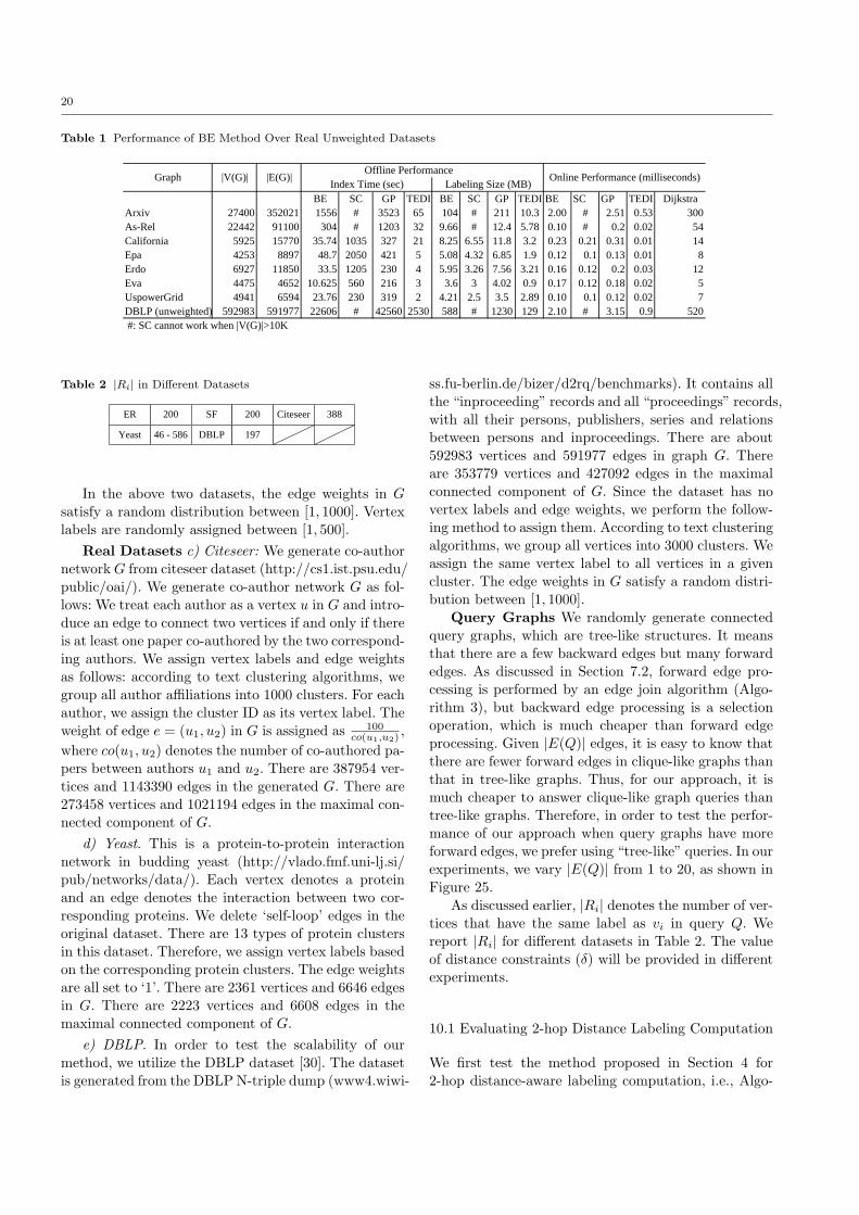
20
Table 1 Performance of BE Method Over Real Unweighted Datasets
BE SC GP TEDI BE SC GP TEDI BE SC GP TEDI DijkstraArxiv 27400 352021 1556 # 3523 65 104 # 211 10.3 2.00 # 2.51 0.53 300As-Rel 22442 91100 304 # 1203 32 9.66 # 12.4 5.78 0.10 # 0.2 0.02 54California 5925 15770 35.74 1035 327 21 8.25 6.55 11.8 3.2 0.23 0.21 0.31 0.01 14Epa 4253 8897 48.7 2050 421 5 5.08 4.32 6.85 1.9 0.12 0.1 0.13 0.01 8Erdo 6927 11850 33.5 1205 230 4 5.95 3.26 7.56 3.21 0.16 0.12 0.2 0.03 12Eva 4475 4652 10.625 560 216 3 3.6 3 4.02 0.9 0.17 0.12 0.18 0.02 5UspowerGrid 4941 6594 23.76 230 319 2 4.21 2.5 3.5 2.89 0.10 0.1 0.12 0.02 7DBLP (unweighted) 592983 591977 22606 # 42560 2530 588 # 1230 129 2.10 # 3.15 0.9 520 #: SC cannot work when |V(G)|>10K
Offline PerformanceOnline Performance (milliseconds)Graph |V(G)| |E(G)| Index Time (sec) Labeling Size (MB)
Table 2 |Ri| in Different Datasets
ER 200 SF 200 Citeseer 388
Yeast 46 - 586 DBLP 197
In the above two datasets, the edge weights in Gsatisfy a random distribution between [1, 1000]. Vertexlabels are randomly assigned between [1, 500].
Real Datasets c) Citeseer: We generate co-authornetwork G from citeseer dataset (http://cs1.ist.psu.edu/public/oai/). We generate co-author network G as fol-lows: We treat each author as a vertex u in G and intro-duce an edge to connect two vertices if and only if thereis at least one paper co-authored by the two correspond-ing authors. We assign vertex labels and edge weightsas follows: according to text clustering algorithms, wegroup all author affiliations into 1000 clusters. For eachauthor, we assign the cluster ID as its vertex label. Theweight of edge e = (u1, u2) in G is assigned as 100
co(u1,u2),
where co(u1, u2) denotes the number of co-authored pa-pers between authors u1 and u2. There are 387954 ver-tices and 1143390 edges in the generated G. There are273458 vertices and 1021194 edges in the maximal con-nected component of G.
d) Yeast. This is a protein-to-protein interactionnetwork in budding yeast (http://vlado.fmf.uni-lj.si/pub/networks/data/). Each vertex denotes a proteinand an edge denotes the interaction between two cor-responding proteins. We delete ‘self-loop’ edges in theoriginal dataset. There are 13 types of protein clustersin this dataset. Therefore, we assign vertex labels basedon the corresponding protein clusters. The edge weightsare all set to ‘1’. There are 2361 vertices and 6646 edgesin G. There are 2223 vertices and 6608 edges in themaximal connected component of G.
e) DBLP. In order to test the scalability of ourmethod, we utilize the DBLP dataset [30]. The datasetis generated from the DBLP N-triple dump (www4.wiwi-
ss.fu-berlin.de/bizer/d2rq/benchmarks). It contains allthe “inproceeding” records and all “proceedings” records,with all their persons, publishers, series and relationsbetween persons and inproceedings. There are about592983 vertices and 591977 edges in graph G. Thereare 353779 vertices and 427092 edges in the maximalconnected component of G. Since the dataset has novertex labels and edge weights, we perform the follow-ing method to assign them. According to text clusteringalgorithms, we group all vertices into 3000 clusters. Weassign the same vertex label to all vertices in a givencluster. The edge weights in G satisfy a random distri-bution between [1, 1000].
Query Graphs We randomly generate connectedquery graphs, which are tree-like structures. It meansthat there are a few backward edges but many forwardedges. As discussed in Section 7.2, forward edge pro-cessing is performed by an edge join algorithm (Algo-rithm 3), but backward edge processing is a selectionoperation, which is much cheaper than forward edgeprocessing. Given |E(Q)| edges, it is easy to know thatthere are fewer forward edges in clique-like graphs thanthat in tree-like graphs. Thus, for our approach, it ismuch cheaper to answer clique-like graph queries thantree-like graphs. Therefore, in order to test the perfor-mance of our approach when query graphs have moreforward edges, we prefer using “tree-like” queries. In ourexperiments, we vary |E(Q)| from 1 to 20, as shown inFigure 25.
As discussed earlier, |Ri| denotes the number of ver-tices that have the same label as vi in query Q. Wereport |Ri| for different datasets in Table 2. The valueof distance constraints (δ) will be provided in differentexperiments.
10.1 Evaluating 2-hop Distance Labeling Computation
We first test the method proposed in Section 4 for2-hop distance-aware labeling computation, i.e., Algo-
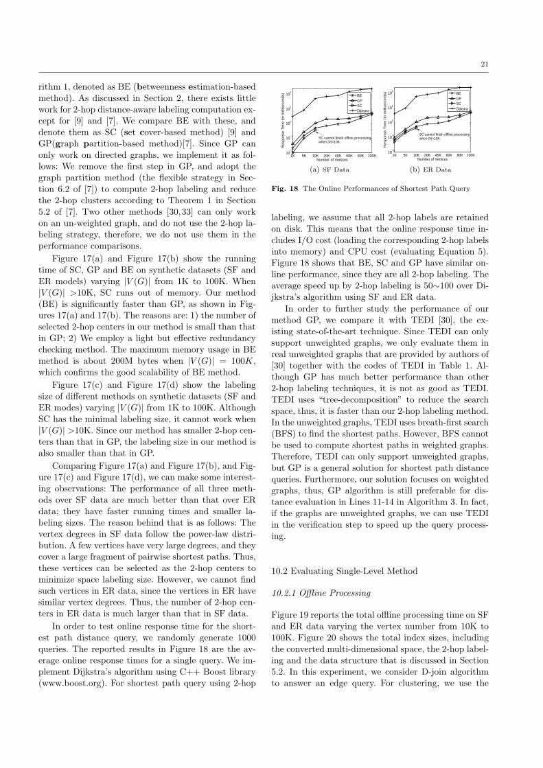
21
rithm 1, denoted as BE (betweenness estimation-basedmethod). As discussed in Section 2, there exists littlework for 2-hop distance-aware labeling computation ex-cept for [9] and [7]. We compare BE with these, anddenote them as SC (set cover-based method) [9] andGP(graph partition-based method)[7]. Since GP canonly work on directed graphs, we implement it as fol-lows: We remove the first step in GP, and adopt thegraph partition method (the flexible strategy in Sec-tion 6.2 of [7]) to compute 2-hop labeling and reducethe 2-hop clusters according to Theorem 1 in Section5.2 of [7]. Two other methods [30,33] can only workon an un-weighted graph, and do not use the 2-hop la-beling strategy, therefore, we do not use them in theperformance comparisons.
Figure 17(a) and Figure 17(b) show the runningtime of SC, GP and BE on synthetic datasets (SF andER models) varying |V (G)| from 1K to 100K. When|V (G)| >10K, SC runs out of memory. Our method(BE) is significantly faster than GP, as shown in Fig-ures 17(a) and 17(b). The reasons are: 1) the number ofselected 2-hop centers in our method is small than thatin GP; 2) We employ a light but effective redundancychecking method. The maximum memory usage in BEmethod is about 200M bytes when |V (G)| = 100K,which confirms the good scalability of BE method.
Figure 17(c) and Figure 17(d) show the labelingsize of different methods on synthetic datasets (SF andER modes) varying |V (G)| from 1K to 100K. AlthoughSC has the minimal labeling size, it cannot work when|V (G)| >10K. Since our method has smaller 2-hop cen-ters than that in GP, the labeling size in our method isalso smaller than that in GP.
Comparing Figure 17(a) and Figure 17(b), and Fig-ure 17(c) and Figure 17(d), we can make some interest-ing observations: The performance of all three meth-ods over SF data are much better than that over ERdata; they have faster running times and smaller la-beling sizes. The reason behind that is as follows: Thevertex degrees in SF data follow the power-law distri-bution. A few vertices have very large degrees, and theycover a large fragment of pairwise shortest paths. Thus,these vertices can be selected as the 2-hop centers tominimize space labeling size. However, we cannot findsuch vertices in ER data, since the vertices in ER havesimilar vertex degrees. Thus, the number of 2-hop cen-ters in ER data is much larger than that in SF data.
In order to test online response time for the short-est path distance query, we randomly generate 1000queries. The reported results in Figure 18 are the av-erage online response times for a single query. We im-plement Dijkstra’s algorithm using C++ Boost library(www.boost.org). For shortest path query using 2-hop
1K 5K 10K 20K 40K 60K 80K 100K10
−2
10−1
100
101
102
Re
spo
nse
Tim
e (
in m
illis
eco
nd
s)
Number of Vertices
BEGPSCDijkstra
SC cannot finish offline processingwhen |V|>10K.
(a) SF Data
1K 5K 10K 20K 40K 60K 80K 100K10
−2
10−1
100
101
102
Re
spo
nse
Tim
e (
in m
illis
eco
nd
s)
Number of Vertices
BEGPSCDijkstra
SC cannot finish offline processingwhen |V|>10K.
(b) ER Data
Fig. 18 The Online Performances of Shortest Path Query
labeling, we assume that all 2-hop labels are retainedon disk. This means that the online response time in-cludes I/O cost (loading the corresponding 2-hop labelsinto memory) and CPU cost (evaluating Equation 5).Figure 18 shows that BE, SC and GP have similar on-line performance, since they are all 2-hop labeling. Theaverage speed up by 2-hop labeling is 50∼100 over Di-jkstra’s algorithm using SF and ER data.
In order to further study the performance of ourmethod GP, we compare it with TEDI [30], the ex-isting state-of-the-art technique. Since TEDI can onlysupport unweighted graphs, we only evaluate them inreal unweighted graphs that are provided by authors of[30] together with the codes of TEDI in Table 1. Al-though GP has much better performance than other2-hop labeling techniques, it is not as good as TEDI.TEDI uses “tree-decomposition” to reduce the searchspace, thus, it is faster than our 2-hop labeling method.In the unweighted graphs, TEDI uses breath-first search(BFS) to find the shortest paths. However, BFS cannotbe used to compute shortest paths in weighted graphs.Therefore, TEDI can only support unweighted graphs,but GP is a general solution for shortest path distancequeries. Furthermore, our solution focuses on weightedgraphs, thus, GP algorithm is still preferable for dis-tance evaluation in Lines 11-14 in Algorithm 3. In fact,if the graphs are unweighted graphs, we can use TEDIin the verification step to speed up the query process-ing.
10.2 Evaluating Single-Level Method
10.2.1 Offline Processing
Figure 19 reports the total offline processing time on SFand ER data varying the vertex number from 10K to100K. Figure 20 shows the total index sizes, includingthe converted multi-dimensional space, the 2-hop label-ing and the data structure that is discussed in Section5.2. In this experiment, we consider D-join algorithmto answer an edge query. For clustering, we use the
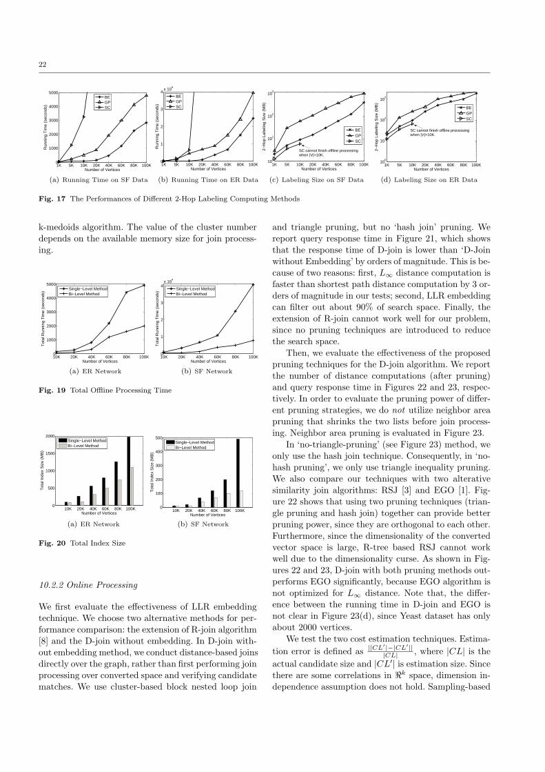
22
1K 5K 10K 20K 40K 60K 80K 100K0
1000
2000
3000
4000
5000
Run
ning
Tim
e (s
econ
ds)
Number of Vertices
BEGPSC
(a) Running Time on SF Data
1K 5K 10K 20K 40K 60K 80K 100K0
1
2
3
4x 10
4
Run
ning
Tim
e (s
econ
ds)
Number of Vertices
BEGPSC
(b) Running Time on ER Data
1K 5K 10K 20K 40K 60K 80K 100K10
0
101
102
103
2−H
op L
abel
ing
Siz
e (M
B)
Number of Vertices
BEGPSC
SC cannot finish offline processingwhen |V|>10K.
(c) Labeling Size on SF Data
1K 5K 10K 20K 40K 60K 80K 100K10
0
101
102
103
2−H
op L
abel
ing
Siz
e (M
B)
Number of Vertices
BEGPSC
SC cannot finish offline processingwhen |V|>10K.
(d) Labeling Size on ER Data
Fig. 17 The Performances of Different 2-Hop Labeling Computing Methods
k-medoids algorithm. The value of the cluster numberdepends on the available memory size for join process-ing.
10K 20K 40K 60K 80K 100K0
1000
2000
3000
4000
5000
Tot
al R
unni
ng T
ime
(sec
onds
)
Number of Vertices
Single−Level MethodBi−Level Method
(a) ER Network
10K 20K 40K 60K 80K 100K0
1
2
3
4x 10
4
Tot
al R
unni
ng T
ime
(sec
onds
)
Number of Vertices
Single−Level MethodBi−Level Method
(b) SF Network
Fig. 19 Total Offline Processing Time
10K 20K 40K 60K 80K 100K0
500
1000
1500
2000
Tot
al In
dex
Siz
e (M
B)
Number of Vertices
Single−Level MethodBi−Level Method
(a) ER Network
10K 20K 40K 60K 80K 100K0
100
200
300
400
500
Tot
al In
dex
Siz
e (M
B)
Number of Vertices
Single−Level MethodBi−Level Method
(b) SF Network
Fig. 20 Total Index Size
10.2.2 Online Processing
We first evaluate the effectiveness of LLR embeddingtechnique. We choose two alternative methods for per-formance comparison: the extension of R-join algorithm[8] and the D-join without embedding. In D-join with-out embedding method, we conduct distance-based joinsdirectly over the graph, rather than first performing joinprocessing over converted space and verifying candidatematches. We use cluster-based block nested loop join
and triangle pruning, but no ‘hash join’ pruning. Wereport query response time in Figure 21, which showsthat the response time of D-join is lower than ‘D-Joinwithout Embedding’ by orders of magnitude. This is be-cause of two reasons: first, L∞ distance computation isfaster than shortest path distance computation by 3 or-ders of magnitude in our tests; second, LLR embeddingcan filter out about 90% of search space. Finally, theextension of R-join cannot work well for our problem,since no pruning techniques are introduced to reducethe search space.
Then, we evaluate the effectiveness of the proposedpruning techniques for the D-join algorithm. We reportthe number of distance computations (after pruning)and query response time in Figures 22 and 23, respec-tively. In order to evaluate the pruning power of differ-ent pruning strategies, we do not utilize neighbor areapruning that shrinks the two lists before join process-ing. Neighbor area pruning is evaluated in Figure 23.
In ‘no-triangle-pruning’ (see Figure 23) method, weonly use the hash join technique. Consequently, in ‘no-hash pruning’, we only use triangle inequality pruning.We also compare our techniques with two alterativesimilarity join algorithms: RSJ [3] and EGO [1]. Fig-ure 22 shows that using two pruning techniques (trian-gle pruning and hash join) together can provide betterpruning power, since they are orthogonal to each other.Furthermore, since the dimensionality of the convertedvector space is large, R-tree based RSJ cannot workwell due to the dimensionality curse. As shown in Fig-ures 22 and 23, D-join with both pruning methods out-performs EGO significantly, because EGO algorithm isnot optimized for L∞ distance. Note that, the differ-ence between the running time in D-join and EGO isnot clear in Figure 23(d), since Yeast dataset has onlyabout 2000 vertices.
We test the two cost estimation techniques. Estima-tion error is defined as ||CL′|−|CL′||
|CL| , where |CL| is theactual candidate size and |CL′| is estimation size. Sincethere are some correlations in <k space, dimension in-dependence assumption does not hold. Sampling-based

23
100 200 300 400 500 100010
0
101
102
Que
ry R
espo
nse
Tim
e (s
ec)
δ
D−JoinD−Join Without EmbeddingExtension of R−join
(a) ER Network
100 200 300 400 500 100010
0
101
102
Que
ry R
espo
nse
Tim
e (s
ec)
δ
D−JoinD−Join Without EmbeddingExtension of R−join
(b) SF Network
10 20 30 40 50 10010
1
102
103
Que
ry R
espo
nse
Tim
e (s
ec)
δ
D−JoinD−Join Without EmbeddingExtension of R−join
(c) Citeseer Network
1 2 3 4 5 610
−1
100
101
Que
ry R
espo
nse
Tim
e (s
ec)
δ
D−JoinD−Join Without EmbeddingExtension of R−join
(d) Yeast Network
Fig. 21 Evaluating Embedding Technique
100 200 300 400 500 1000
2.6
2.8
3
3.2
3.4
3.6
3.8
4
4.2x 10
4
Num
ber
of D
ista
nce
Com
puta
tion
δ
D−joinNo−triangle−pruningNo−hash−pruningRSJEGO
(a) ER Network
100 200 300 400 500 1000
2.6
2.8
3
3.2
3.4
3.6
3.8
4
4.2x 10
4
Num
ber
of D
ista
nce
Com
puta
tion
δ
D−joinNo−triangle−pruningNo−hash−pruningRSJEGO
(b) SF Network
10 20 30 40 50 1002.2
2.4
2.6
2.8
3
3.2
3.4
3.6
3.8x 10
5
Num
ber
of D
ista
nce
Com
puta
tion
δ
D−joinNo−triangle−pruningNo−hash−pruningRSJEGO
(c) Citeseer Network
1 2 3 4 5 61
2
3
4
5
6
7
8
x 104
Num
ber
of D
ista
nce
Com
puta
tion
δ
D−joinNo−triangle−pruningNo−hash−pruningRSJEGO
(d) Yeast Network
Fig. 22 Number of Distance Computation
100 200 300 400 500 100010
−1
100
101
Que
ry R
espo
nse
Tim
e (s
ec)
δ
D−joinNo−triangle−pruningNo−hash−pruningRSJEGO
(a) ER Network
100 200 300 400 500 1000100
101
Que
ry R
espo
nse
Tim
e (s
ec)
δ
D-joinNo-triangle-pruningNo-hash-pruningRSJEGO
(b) SF Network
10 20 30 40 50 100
102
Que
ry R
espo
nse
Tim
e (s
ec.)
δ
D−joinNo−triagnle−pruingNo−hash−pruningRSJEGO
(c) Citeseer Network
10 20 30 40 50 1000
0.5
1
1.5
2
2.5
3
3.5
4
Que
ry R
espo
nse
Tim
e (s
ec)
δ
D-joinNo-triangle-pruningNo-hash-pruningRSJEGO
(d) Yeast Network
Fig. 23 Edge Query Response Time
100 200 300 400 500 10000
5
10
15
20
25
Err
or R
aio
δ
Dimension−independent assumptionSampling
(a) ER Network
100 200 300 400 500 10000
5
10
15
20
25
Err
or R
aio
δ
Dimension−independent assumptionSampling
(b) SF Network
10 20 30 40 50 1000
5
10
15
20
25
30
35
40
Err
or R
aio
δ
Dimension−independent assumptionSampling
(c) Citeseer Network
1 2 3 4 5 60
1
2
3
4
5
6
7
8
Err
or R
aio
δ
Dimension−independent assumptionSampling
(d) Yeast Network
Fig. 24 Cost Estimation
technique can capture data distribution in <k space,thus, it can provide better estimation, as shown in Fig-ure 24.
We test the performance of MD-join algorithm. Wealso evaluate the effectiveness of neighbor-area prun-ing technique and join order selection method. In this
experiment, we fix the distance constraint δ, and vary|E(Q)| from 2 to 20. In ‘without neighbor area prun-ing’, we do not reduce the search space by neighbor areapruning, but we still use join order selection methodto select a cheap query plan. In ‘no join order selec-tion’, we randomly define the join order for the MD-
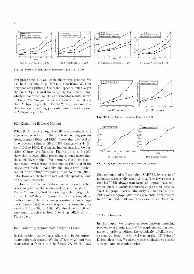
24
2 3 4 5 10 15 200
5
10
15
20
Que
ry R
espo
nse
Tim
e (s
ec)
|E(Q)|
MD−JoinNo Join Order SelectionNo Neighbor Area Pruning
(a) ER Network, δ = 200
2 3 4 5 10 15 200
5
10
15
Que
ry R
espo
nse
Tim
e (s
ec)
|E(Q)|
MD−JoinNo Join Order SelectionNo Neighbor Area Pruning
(b) SF Network, δ = 200
2 3 4 5 10 15 200
50
100
150
200
Que
ry R
espo
nse
Tim
e (s
ec)
|E(Q)|
MD−JoinNo Join Order SelectionNo Neighbor Area Pruning
(c) Citeseer Network, δ = 20
2 3 4 5 10 15 200
0.5
1
1.5
2
Que
ry R
espo
nse
Tim
e (s
ec)
|E(Q)|
MD−JoinNo Join Order SelectionNo Neighbor Area Pruning
(d) Yeast Network, δ = 2
Fig. 25 Pattern Match Query Response Time VS. |E(Q)|
join processing, but we use neighbor area pruning. Weuse both techniques in MD-join algorithm. Withoutneighbor area pruning, the search space is much largerthan in MD-join algorithm using neighbor area pruning,which is confirmed by the experimental results shownin Figure 25. ‘No join order selection’ is much slowerthan MD-join algorithm. Figure 25 also demonstratesthat randomly defining join order cannot work as wellas MD-join algorithm.
10.3 Evaluating Bi-Level Method
When |V (G)| is very large, the offline processing is veryexpensive, especially in the graph embedding process(recall Figures 19(a) and 19(b)). We evaluate bi-level of-fline processing time on SF and ER data varying |V (G)|from 10K to 100K. During the implementation, we par-tition G into 10 subgraphs. Figures 19(a) and 19(b)show that bi-level offline processing is much faster thanthe single-level method. Furthermore, the index size inthe second-level method is also smaller than that in thesingle-level method. Actually, the single-level methodcannot finish offline processing in 48 hours on DBLPdata. However, the bi-level method only spends 5 hourson the same datasets.
However, the online performance of bi-level methodis not as good as the single-level version, as shown inFigure 26. We only test bD-Join algorithm (Algorithm9) over DBLP data in Figure 27, since the single-levelmethod cannot finish offline processing on such largedata. Figure 28(a) shows the query response time forvarying δ from 200 to 1000. We also fix δ = 200 andvary query graph size from 2 to 6 on DBLP data inFigure 28(b).
10.4 Evaluating Approximate Subgraph Search
In this section, we evaluate Algorithm 10 for approx-imate subgraph search. We fix |E(Q)| = 20 and varyrelax ratio ∆ from 1 to 5 in Figure 28, which shows
1K 2K 4K 6K 8K 10K
1
2
3
4
5
6
7
8
9
Que
ry R
espo
nse
Tim
e (s
ec)
Signle−Level D−JoinBi−Level D−Join
(a) ER Network
1K 2K 4K 6K 8K 10K0
1
2
3
4
5
6
7
Que
ry R
espo
nse
Tim
e (s
ec)
Signle−Level D−JoinBi−Level D−Join
(b) SF Network
Fig. 26 Edge Query Response Time, δ = 200
100 200 400 600 800 100060
80
100
120
140
Que
ry R
espo
nse
Tim
e (s
ec)
δ
Bi−Level D−Join
(a) Edge Query
1 2 3 4 5 660
80
100
120
140
160
180
200
220
Que
ry R
espo
nse
Tim
e (s
ec)
|E(Q)|
Bi−Level D−Join
(b) Pattern Query
Fig. 27 Query Response Time Over DBLP data
that our method is faster than SAPPER by orders ofmagnitude, especially when ∆ > 3. The key reason isthat SAPPER always transforms an approximate sub-graph query allowing for missed edges to all possibleexact subgraph queries. Obviously, the number of pos-sible exact subgraph queries is exponential with respectto ∆. Thus, SAPPER cannot work well when ∆ is large.
11 Conclusions
In this paper, we propose a novel pattern matchingproblem over a large graph G by graph embedding tech-nique. In order to address the complexity of offline pro-cessing, we design the bi-level version (i.e., bD-Join) ofD-Join algorithm. We also propose a solution to answerapproximate subgraph queries.
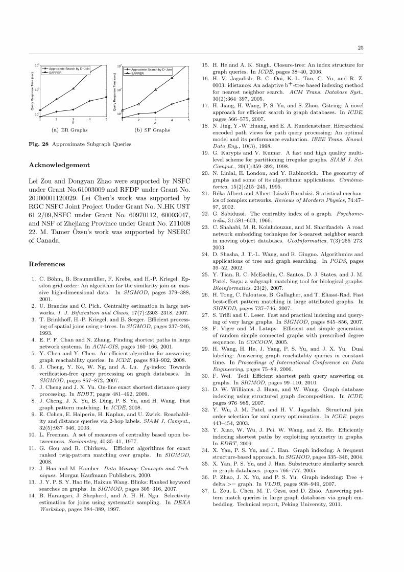
25
1 2 3 4 5
101
102
103
Que
ry R
espo
nse
Tim
e (s
ec)
∆
Approximte Search by D−JoinSAPPER
(a) ER Graphs
1 2 3 4 5
101
102
103
Que
ry R
espo
nse
Tim
e (s
ec)
∆
Approximte Search by D−JoinSAPPER
(b) SF Graphs
Fig. 28 Approximate Subgraph Queries
Acknowledgement
Lei Zou and Dongyan Zhao were supported by NSFCunder Grant No.61003009 and RFDP under Grant No.20100001120029. Lei Chen’s work was supported byRGC NSFC Joint Project Under Grant No. N HK UST61 2/09,NSFC under Grant No. 60970112, 60003047,and NSF of Zhejiang Province under Grant No. Z1100822. M. Tamer Ozsu’s work was supported by NSERCof Canada.
References
1. C. Bohm, B. Braunmuller, F. Krebs, and H.-P. Kriegel. Ep-silon grid order: An algorithm for the similarity join on mas-
sive high-dimensional data. In SIGMOD, pages 379–388,2001.
2. U. Brandes and C. Pich. Centrality estimation in large net-
works. I. J. Bifurcation and Chaos, 17(7):2303–2318, 2007.
3. T. Brinkhoff, H.-P. Kriegel, and B. Seeger. Efficient process-
ing of spatial joins using r-trees. In SIGMOD, pages 237–246,1993.
4. E. P. F. Chan and N. Zhang. Finding shortest paths in large
network systems. In ACM-GIS, pages 160–166, 2001.
5. Y. Chen and Y. Chen. An efficient algorithm for answering
graph reachability queries. In ICDE, pages 893–902, 2008.
6. J. Cheng, Y. Ke, W. Ng, and A. Lu. fg-index: Towardsverification-free query processing on graph databases. In
SIGMOD, pages 857–872, 2007.
7. J. Cheng and J. X. Yu. On-line exact shortest distance query
processing. In EDBT, pages 481–492, 2009.8. J. Cheng, J. X. Yu, B. Ding, P. S. Yu, and H. Wang. Fast
graph pattern matching. In ICDE, 2008.9. E. Cohen, E. Halperin, H. Kaplan, and U. Zwick. Reachabil-
ity and distance queries via 2-hop labels. SIAM J. Comput.,
32(5):937–946, 2003.
10. L. Freeman. A set of measures of centrality based upon be-tweenness. Sociometry, 40:35–41, 1977.
11. G. Gou and R. Chirkova. Efficient algorithms for exact
ranked twig-pattern matching over graphs. In SIGMOD,2008.
12. J. Han and M. Kamber. Data Mining: Concepts and Tech-
niques. Morgan Kaufmann Publishers, 2000.
13. J. Y. P. S. Y. Hao He, Haixun Wang. Blinks: Ranked keywordsearches on graphs. In SIGMOD, pages 305–316, 2007.
14. B. Harangsri, J. Shepherd, and A. H. H. Ngu. Selectivityestimation for joins using systematic sampling. In DEXA
Workshop, pages 384–389, 1997.
15. H. He and A. K. Singh. Closure-tree: An index structure forgraph queries. In ICDE, pages 38–40, 2006.
16. H. V. Jagadish, B. C. Ooi, K.-L. Tan, C. Yu, and R. Z.
0003. idistance: An adaptive b+-tree based indexing methodfor nearest neighbor search. ACM Trans. Database Syst.,
30(2):364–397, 2005.17. H. Jiang, H. Wang, P. S. Yu, and S. Zhou. Gstring: A novel
approach for efficient search in graph databases. In ICDE,
pages 566–575, 2007.18. N. Jing, Y.-W. Huang, and E. A. Rundensteiner. Hierarchical
encoded path views for path query processing: An optimal
model and its performance evaluation. IEEE Trans. Knowl.Data Eng., 10(3), 1998.
19. G. Karypis and V. Kumar. A fast and high quality multi-
level scheme for partitioning irregular graphs. SIAM J. Sci.Comput., 20(1):359–392, 1998.
20. N. Linial, E. London, and Y. Rabinovich. The geometry of
graphs and some of its algorithmic applications. Combina-torica, 15(2):215–245, 1995.
21. Reka Albert and Albert-Laszlo Barabasi. Statistical mechan-
ics of complex networks. Reviews of Mordern Physics, 74:47–97, 2002.
22. G. Sabidussi. The centrality index of a graph. Psychome-
trika, 31:581–603, 1966.23. C. Shahabi, M. R. Kolahdouzan, and M. Sharifzadeh. A road
network embedding technique for k-nearest neighbor search
in moving object databases. GeoInformatica, 7(3):255–273,2003.
24. D. Shasha, J. T.-L. Wang, and R. Giugno. Algorithmics andapplications of tree and graph searching. In PODS, pages
39–52, 2002.25. Y. Tian, R. C. McEachin, C. Santos, D. J. States, and J. M.
Patel. Saga: a subgraph matching tool for biological graphs.
Bioinformatics, 23(2), 2007.26. H. Tong, C. Faloutsos, B. Gallagher, and T. Eliassi-Rad. Fast
best-effort pattern matching in large attributed graphs. In
SIGKDD, pages 737–746, 2007.27. S. Trißl and U. Leser. Fast and practical indexing and query-
ing of very large graphs. In SIGMOD, pages 845–856, 2007.28. F. Viger and M. Latapy. Efficient and simple generation
of random simple connected graphs with prescribed degreesequence. In COCOON, 2005.
29. H. Wang, H. He, J. Yang, P. S. Yu, and J. X. Yu. Dual
labeling: Answering graph reachability queries in constanttime. In Proceedings of International Conference on Data
Engineering, pages 75–89, 2006.30. F. Wei. Tedi: Efficient shortest path query answering on
graphs. In SIGMOD, pages 99–110, 2010.31. D. W. Williams, J. Huan, and W. Wang. Graph database
indexing using structured graph decomposition. In ICDE,pages 976–985, 2007.
32. Y. Wu, J. M. Patel, and H. V. Jagadish. Structural joinorder selection for xml query optimization. In ICDE, pages
443–454, 2003.33. Y. Xiao, W. Wu, J. Pei, W. Wang, and Z. He. Efficiently
indexing shortest paths by exploiting symmetry in graphs.
In EDBT, 2009.34. X. Yan, P. S. Yu, and J. Han. Graph indexing: A frequent
structure-based approach. In SIGMOD, pages 335–346, 2004.35. X. Yan, P. S. Yu, and J. Han. Substructure similarity search
in graph databases. pages 766–777, 2005.36. P. Zhao, J. X. Yu, and P. S. Yu. Graph indexing: Tree +
delta >= graph. In VLDB, pages 938–949, 2007.37. L. Zou, L. Chen, M. T. Ozsu, and D. Zhao. Answering pat-
tern match queries in large graph databases via graph em-
bedding. Technical report, Peking University, 2011.
Recommended