ANOVA approaches to Repeated Measures
• univariate repeated-measures ANOVA (chapter 2)
• repeated measures MANOVA (chapter 3)
Assumptions
• Interval measurement and normally distributed errors(homogeneous across groups) - transformation may help
• Group comparisons
– estimation and comparison of group means
– not informative about individual growth
• Fixed time points
– time treated as classification variable
– timepoints can be evenly or unevenly spaced
1

• Better suited for short-term or moderate changeesp. true for trend or growth-curve analysis
• LS techniques adversely affected by outliers
• Missing data
– ANOVA can handle some - unbalanced ANOVA
– MANOVA can’t handle any
• Variance-covariance structure for yi
– compound symmetry for ANOVA
– unstructured for MANOVA
2

Univariate Repeated Measures ANOVA
One-sample case: randomized block ANOVA
yij = µ + πi + τj + eij (i = 1, . . . , N ; j = 1, . . . , n)
• µ = grand mean
• πi = individual difference component for subject i(constant over time)
• τj = effect of time - same for all subjects
• eij = error for subject i and time j
Random components
• πi ∼ N(0, σ2π) subjects random; between-subjects variance
• eij ∼ N(0, σ2e) within-subjects variance
3

Data layout
timepointsubject 1 2 . . . n
1 y11 y12 . . . y1n
2 y21 y22 . . . y2n
. . . . . . .
. . . . . . .
N yN1 yN2 . . . yNn
• one observation per cell
• similar to randomized block design with subject as block
• identical to paired-t test when n = 2
4

Model assumptions
n∑
j=1τj = 0 (n − 1 df for Time)
E(yij) = µ + τj
V (yij) = V (µ + τj + πi + eij) = σ2π + σ2
e
C(yij, yi′j) = 0 for i 6= i′ (different subjects)
C(yij, yij′) = σ2π for j 6= j′ (same subject)
5
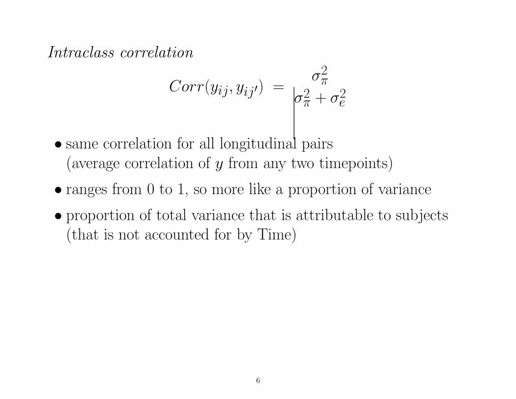
Intraclass correlation
Corr(yij, yij′) =σ2π
σ2π + σ2
e
• same correlation for all longitudinal pairs(average correlation of y from any two timepoints)
• ranges from 0 to 1, so more like a proportion of variance
• proportion of total variance that is attributable to subjects(that is not accounted for by Time)
6

Compound symmetry structure ofvariance-covariance matrix
Σyi=
σ2e + σ2
π σ2π σ2
π . . . σ2π
σ2π σ2
e + σ2π σ2
π . . . σ2π
. . . . . . . . . . . . . . .
σ2π . . . σ2
π σ2e + σ2
π σ2π
σ2π σ2
π . . . σ2π σ2
e + σ2π
• variance homogeneous across time: σ2e + σ2
π
• covariances homogenous across time: σ2π
correlation = σ2π/(σ2
e + σ2π)
7
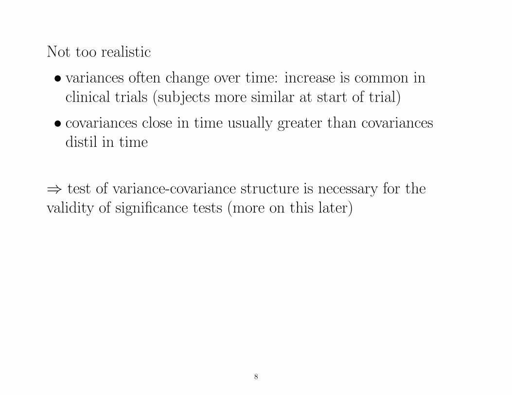
Not too realistic
• variances often change over time: increase is common inclinical trials (subjects more similar at start of trial)
• covariances close in time usually greater than covariancesdistil in time
⇒ test of variance-covariance structure is necessary for thevalidity of significance tests (more on this later)
8
9

ANOVA table: subjects random and time fixed (balanced)
Source df SS MS E(MS)
Subjects N − 1 SSS = n ∑Ni=1(yi. − y..)
2 SSSN−1 σ2
e + nσ2π
Time n − 1 SST = N ∑nj=1(y.j − y..)
2 SSTn−1
σ2e + N ∑(τj − τ.)
2
Residual (N − 1) SSR = ∑Ni=1
∑nj=1(yij
SSR(N−1)(n−1)
σ2e
×(n − 1) −yi. − y.j + y..)2
total Nn − 1 SSy = ∑Ni=1
∑nj=1(yij − y..)
2
• y.. = grand mean (averaged over time and subjects)
• yi. = subject mean (i = 1, . . . , N)
• y.j = timepoint mean (j = 1, . . . , n)
10
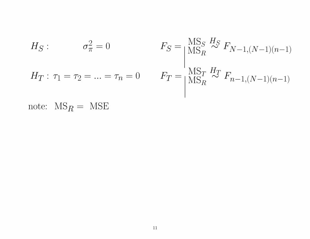
HS : σ2π = 0 FS = MSS
MSR
HS∼ FN−1,(N−1)(n−1)
HT : τ1 = τ2 = ... = τn = 0 FT = MSTMSR
HT∼ Fn−1,(N−1)(n−1)
note: MSR = MSE
11

Intraclass correlation - relative magnitude of σ2π
• usually assume σ2π > 0
• want to quantify degree of subject effect
r =σ2π
σ2π + σ2
e
• σ2π = ( MSS − MSR) / n
– when MSS ≤ MSR, then σ2π = 0
• σ2e = MSR
12

• proportion of (unexplained) variation due to subjects
• as subjects’ data are highly correlated, r gets large
• can vary depending on model covariates
13

Contrasts for time differences
• HT : τ1 = τ2 = ... = τn = 0 is a very global test
• contrasts address more specific time-related comparisions
• Hj′ : Lj′ = ∑nj=1 cj′j µ.j = 0
Define the (estimated) contrast of the timepoint means as:
Lj′ =n∑
j=1cj′j y.j j′ = 1, . . . , n − 1
n∑
j=1cj′j = 0
e.g., suppose that there are two timepoints, then
H1 : µ1 = µ2 ⇐⇒ H1 : µ1−µ2 = 0 ⇐⇒ H1 : (1)µ1+(−1)µ2 = 0
here, c11 = 1 and c12 = −1 and H1 is tested by the contrast:
L1 = (1)y1 + (−1)y2
14

suppose that there are three timepoints and interest is in:
H1 : µ1 = µ2 ⇐⇒ H1 : (1)µ1 + (−1)µ2 + (0)µ3 = 0
H2 : µ1 = µ3 ⇐⇒ H2 : (1)µ1 + (0)µ2 + (−1)µ3 = 0
these would be tested by the contrasts:
L1 = (1)y1 + (−1)y2 + (0)y3
L2 = (1)y1 + (0)y2 + (−1)y3
15

Inference for contrasts Hj′ : Lj′ = ∑nj=1 cj′j µ.j = 0
SSj′ = MSj′ = NL2j′ /
n∑
j=1c2j′j
Fj′ =MSj′
MSR
Hj′∼ F1,(N−1)(n−1)
tj′ =Lj′√√√√√√√√√ MSR
∑nj=1
c2j′jN
Hj′∼ t(N−1)(n−1)
If the set of n − 1 contrasts are orthogonal, then
SST =n−1∑
j′=1SSj′
⇒ independent partitioning of the variation due to time
16

Trend Analysis - orthogonal polynomials
• characterize n− 1 time effects as n− 1 orthogonal polynomials
• tables in Bock (1975), Draper & Smith (1981), Fleiss (1986)
For example, the n − 1 × n contrast matrix for n = 4 is
C =
−3 −1 1 3 ... ÷√
20
1 −1 −1 1 ... ÷√
4
−1 3 −3 1 ... ÷√
20
linearquadcubic
• orthogonal (and orthonormal with ÷)
• useful for determining “degree” of change across time
• generalized for unequally spaced timepoints
• can specify fewer than n − 1 contrasts
17

Purely linear change
L1 = (−3)1 + (−1)2 + (1)3 + (3)4 = 10/√
20 = 2.24
L2 = (1)1 + (−1)2 + (−1)3 + (1)4 = 0
L3 = (−1)1 + (3)2 + (−3)3 + (1)4 = 0
18

Purely quadratic change
L1 = (−3)1 + (−1)2 + (1)2 + (3)1 = 0
L2 = (1)1 + (−1)2 + (−1)2 + (1)1 = −2/√
4 = −1
L3 = (−1)1 + (3)2 + (−3)2 + (1)1 = 0
19
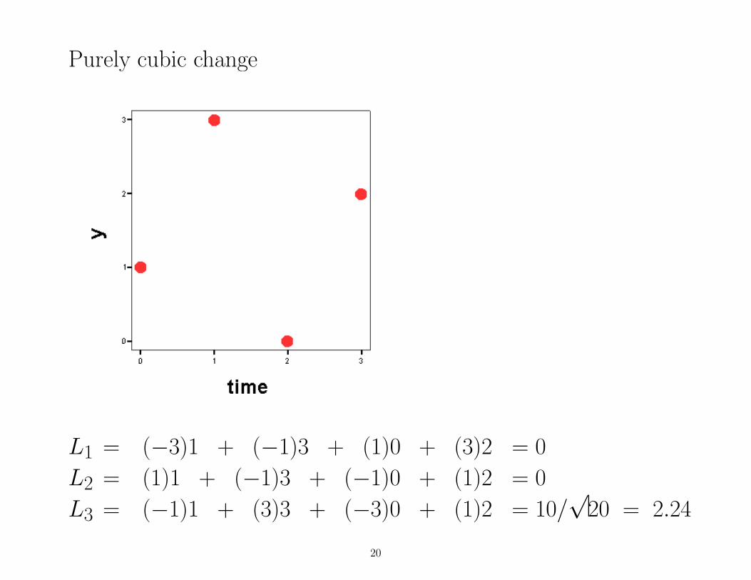
Purely cubic change
L1 = (−3)1 + (−1)3 + (1)0 + (3)2 = 0
L2 = (1)1 + (−1)3 + (−1)0 + (1)2 = 0
L3 = (−1)1 + (3)3 + (−3)0 + (1)2 = 10/√
20 = 2.24
20

21

22

23

Example 2b: IML code for generating orthogonal polynomialcontrast matrix (SAS code and output)
http://www.uic.edu/classes/bstt/bstt513/orthpoly.txt
TITLE ’Generating Orthogonal Polynomial Matrix’;
PROC IML;
xraw = { 1 1 1 1 ,
0 1 2 3 ,
0 1 4 9 ,
0 1 8 27 } ;
xorth =T(INV(ROOT(xraw∗T(xraw))))∗xraw;PRINT ’Matrix of Time Polynomials’, xraw
[FORMAT=10.4];
PRINT ’Orthonormalized Matrix of Time
Polynomials’, xorth [FORMAT=10.4];
24

Generating Orthogonal Polynomial Matrix
Matrix of Time Polynomials
XRAW
1.0000 1.0000 1.0000 1.0000
0.0000 1.0000 2.0000 3.0000
0.0000 1.0000 4.0000 9.0000
0.0000 1.0000 8.0000 27.0000
Orthonormalized Matrix of Time Polynomials
XORTH
0.5000 0.5000 0.5000 0.5000
-0.6708 -0.2236 0.2236 0.6708
0.5000 -0.5000 -0.5000 0.5000
-0.2236 0.6708 -0.6708 0.2236
25

Change relative to 1st timepoint (e.g., baseline)
C =
−1 1 0 0−1 0 1 0−1 0 0 1
for T2-T1, T3-T1, T4-T1, respectively
• not orthogonal
• sometimes called simple contrasts
• other cell can be reference cell (e.g., last time)
26

Consectutive time comparisons (profile contrasts)
C =
−1 1 0 00 −1 1 00 0 −1 1
for T2-T1, T3-T2, T4-T3, respectively
• not orthogonal
• useful for identifying when change begins (and ends)
27

Contrasting timepoint to mean of subsequenttimepoints (Helmert contrasts)
C =
1 −1/3 −1/3 −1/30 1 −1/2 −1/20 0 1 −1
for T1 vs avg of T2, T3, T4; T2 vs avg of T3, T4; T3 vs T4
• orthogonal
• useful for “ordered” tests
28

Contrasting each timepoint to mean of others(Deviational contrasts)
C =
1 −1/3 −1/3 −1/3−1/3 1 −1/3 −1/3−1/3 −1/3 1 −1/3
for T1 vs avg of T2, T3, T4; T2 vs avg of T1, T3, T4; T3 vs avgof T1, T2, T4
• not orthogonal
• useful for “vague knowledge” situation
• omitted timepoint can be other than last
29

Testing Time Differences
multiple comparisons issue, though often n − 1 contrasts can bespecified a-priori
• Bonferroni corrected α level
– α∗ = α/(n − 1)
• Fisher protected test logic
– use α, but only apply when HT : τ1 = τ2 = ... = τn = 0 isrejected
• For orthogonal polynomials
– start with highest-order polynomial and eliminate(simplify) as polynomials are non-significant
Hummel & Sligo (1971) support Fisher protected test if n is nottoo large
30

Also, from Rosner (1995) Fundamentals of Biostatistics, p. 319:
If a few linear contrasts, which have been specified inadvance, are to be tested, then it may not be necessary touse a multiple-comparisons procedure, since if suchprocedures are used, there will be less power to detectdifferences for linear contrasts whose means are trulydifferent from zero. Conversely, if many contrasts are to betested, which have not been specified before looking at thedata, then multiple-comparisons procedures may be usefulin protecting against declaring too many significantdifferences.
31

Example 2a: Analysis of vocabulary data from Bock (1975)using univariate repeated measures ANOVA(SAS code and output)
http://tigger.uic.edu/∼hedeker/bockv.txt
32
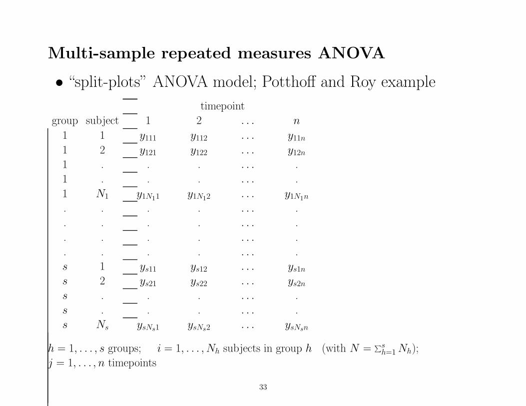
Multi-sample repeated measures ANOVA
• “split-plots” ANOVA model; Potthoff and Roy example
timepoint
group subject 1 2 . . . n
1 1 y111 y112 . . . y11n
1 2 y121 y122 . . . y12n
1 . . . . . . .
1 . . . . . . .
1 N1 y1N11 y1N12 . . . y1N1n
. . . . . . . .
. . . . . . . .
. . . . . . . .
. . . . . . . .
s 1 ys11 ys12 . . . ys1n
s 2 ys21 ys22 . . . ys2n
s . . . . . . .
s . . . . . . .
s Ns ysNs1 ysNs2 . . . ysNsn
h = 1, . . . , s groups; i = 1, . . . , Nh subjects in group h (with N =∑s
h=1 Nh);
j = 1, . . . , n timepoints
33

Model
yhij = µ + γh + τj + (γτ )hj + πi(h) + ehij
• µ = grand mean
• γh = effect of group h (∑h γh = 0)
• τj = effect of time j (∑j τj = 0)
• (γτ )hj = interaction of time j by grp h [∑h
∑j(γτ )hj = 0]
• πi(h) = individual difference component for sub i in grp h
• ehij = error for subject i in group h at time j
• πi(h) ∼ N(0, σ2π)
• ehij ∼ N(0, σ2e)
⇒ compound symmetry structure for V (yi)
34

ANOVA table: subjects random and group & time fixed(balanced in terms of n, not in terms of Nh)
Source df SS MS E(MS)
Group s − 1 SSG = n∑s
h=1 Nh (yh.. − y...)2 SSG
s−1σ2
e + nσ2π + DG
Time n − 1 SST = N∑n
j=1(y..j − y...)2 SST
n−1σ2
e + DT
Group (s − 1) SSGT =∑s
h=1∑n
j=1 Nh (yh.jSSGT
(s−1)(n−1)σ2
e + DGT
× Time ×(n − 1) −yh.. − y..j + y...)2
Subjects N − s SSS(G) = n∑s
h=1∑Nh
i=1(yhi. − yh..)2 SSS(G)
N−sσ2
e + nσ2π
in Grps
Residual (N − s) SSR =∑s
h=1∑Nh
i=1∑n
j=1 (yhijSSR
(N−s)(n−1) σ2e
×(n − 1) −yh.j − yhi. + yh..)2
total Nn − 1 SSy =∑s
h=1∑Nh
i=1∑n
j=1(yhij − y...)2
35

• h = 1, . . . , s groups
• i = 1, . . . , Nh subjects in group h (with N = ∑sh=1 Nh)
• j = 1, . . . , n timepoints
DG, DT , and DGT represent differences among groups,timepoints, and group × time interaction, respectively
36

Testing for Group by Time interaction
HGT : DGT = 0 FGT =MSGT
MSR
HGT∼ F(s−1)(n−1),(N−s)(n−1)
Usually, test of primary interest
If rejected,
• group differences are not the same across time
• group curves across time are not parallel
• group and time effects are confounded with the interaction &can’t be separately tested (or estimated)
37

38
39

40

41

If HGT : DGT = 0 accepted,
HT : τ1 = τ2 = . . . = τn = 0 FT =MST
MSR
HT∼ Fn−1,(N−s)(n−1)
HG : γ1 = γ2 = . . . = γs = 0 FG =MSG
MSS(G)
HG∼ Fs−1,N−s
HT and HG are separately and independently testable
42

Testing for Subject effect
HS(G) : σ2π = 0 FS(G) =
MSS(G)
MSR
HS(G)∼ FN−s,(N−s)(n−1)
• usually assume σ2π > 0
• estimate intraclass correlation
– r = σ2π/(σ2
π + σ2e)
– proportion of (unexplained) variation due to subjects
43

Contrasts for time effects
Again, it’s advantageous to characterize time and group by timeeffects using time-related contrasts
• e.g., orthogonal polynomials
• Fisher protected tests or Bonferroni correction for(n− 1)(s− 1) group by time contrasts, or n− 1 time contrasts
44

Orthogonal Polynomial Partition of SS
C4 =
−3 −1 1 3 ... ÷√
20
1 −1 −1 1 ... ÷√
4
−1 3 −3 1 ... ÷√
20
c1c2c3
Time df SSlinear 1 SST1
= N c1 y..j y′..j c′1
quadratic 1 SST2= N c2 y..j y′
..j c′2. . .(n − 1)th 1 SSTn−1
= N cn−1 y..j y′..j c′n−1
n − 1 SST
• y..j = n × 1 vector of timepoint means
• cj = 1 × n vector of contrasts of order j
45

FTn−1= SSTn−1
/ MSR
. . .
FT1= SST1
/ MSR
Determine polynomial of least degree working backwards
46

G × T df SSlinear s − 1 SSGT1
= ∑h Nh c1 yh.j y′
h.j c′1 − SST1
quadratic s − 1 SSGT2= ∑
h Nh c2 yh.j y′h.j c′2 − SST2
. . .(n − 1)th s − 1 SSGTn−1
= ∑h Nh cn−1 yh.j y′
h.j c′n−1
− SSTn−1
(s − 1) SSGT×(n − 1)
• yh.j = n × 1 vector of timepoint means for group h
• cj = 1 × n vector of contrasts of order j
47

FGTn−1=
SSGTn−1/ (s − 1)
MSR. . .
. . .
FGT1=
SSGT1/ (s − 1)
MSR
Determine polynomial of least degree working backwards
48

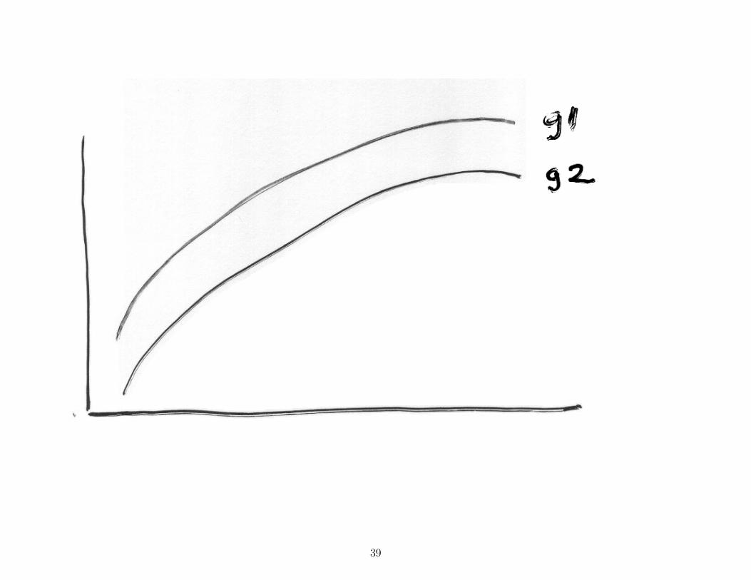
Example 2c: Analysis of Pothoff & Roy data usingunivariate repeated measures ANOVA model with twogroups (boys and girls). Includes a plot of the means acrosstime for the two groups. (SAS code and output)
http://tigger.uic.edu/∼hedeker/pothoff0.txt
49
Example 2d: Analysis of Pothoff & Roy data usingunivariate repeated measures ANOVA. This analysis is for amain effects model - no group by time interaction. (SAScode and output)
http://tigger.uic.edu/∼hedeker/pothoffb.txt
50

SAS code for univariate repeated measures ANOVAwith more than 2 groups
suppose 3 groups (control, tx1, tx2) and interest in comparisonsto control
control tx1 tx2contrast 1 1 -1 0contrast 2 1 0 -1
suppose 4 timepoints and interest in trend analysis
time1 time2 time3 time4linear -3 -1 1 3quad 1 -1 -1 1cubic -1 3 -3 1
51

PROC GLM;
CLASS group time subject;
MODEL y = group subject(group) time group*time;
TEST H=group E=subject(group);
CONTRAST ’tx1’ group 1 -1 0;
CONTRAST ’tx2’ group 1 0 -1;
CONTRAST ’linear’ time -3 -1 1 3;
CONTRAST ’quad’ time 1 -1 -1 1;
CONTRAST ’cubic’ time -1 3 -3 1;
CONTRAST ’tx1*lin’ group*time
-3 -1 1 3 3 1 -1 -3 0 0 0 0;
CONTRAST ’tx2*lin’ group*time
-3 -1 1 3 0 0 0 0 3 1 -1 -3;
. . . . . . . . .
CONTRAST ’tx2*cub’ group*time
-1 3 -3 1 0 0 0 0 1 -3 3 -1;
52

Compound Symmetry and Sphericity
For both univariate RB and SP ANOVA models
V (yi) = σ2π1n1
′n + σ2
eIn
Compound symmetry (CS) structure
V (yij) = σ2π + σ2
e ∀ j
C(yij, yij′) = σ2π ∀ j and j′ (j 6= j′)
• ρ(yij, yij′) = σ2π / (σ2
π + σ2e) = ICC
• Highly restrictive assumption and often unrealistic(especially as n gets large)
53

• CS is special case of more general situation, sphericity, underwhich F -tests for time-related terms from ANOVA models arevalid
– if sphericity holds, then F -tests are valid
– if sphericity doesn’t hold, then F -tests are generally tooliberal
54

Sphericity - sometimes called circularity
• Can be expressed in different ways
• e.g., variances of all pairwise differences between variables areequal
V (yij − yij′) = V (yij) + V (yij′) − 2C(yij, yij′)
= constant ∀ j and j′
• CS is a special case of sphericity
V (yij) = σ2π + σ2
e constant
C(yij, yij′) = σ2π constant
55

More generally, Crowder and Hand (1990, page 50) note:
MS ratios derived by the univariate approach follow exactF -distributions if and only if the covariance matrix of theorthonormal contrasts has equal variances and zerocovariances
C(n−1)×n
V (yi)n×n
C ′
n×(n−1)
= constant In−1(n−1)×(n−1)
• where C is matrix of orthonormal polynomials
• test in SAS using multivariate data setup
56

Running univariate repeated-measures ANOVA viamultivariate setup
• univariate setup:
group subject time y1 1 1 y1111 1 2 y1121 1 3 y113
• multivariate setup:group subject y1 y2 y3
1 1 y111 y112 y113
57

DATA unidat;
INPUT subject time y;
DATALINES;
1 1 1
1 2 2
1 3 3
2 1 4
2 2 5
2 3 6
;
DATA multdat;
ARRAY yv(3) y1 y2 y3;
DO time = 1 TO 3;
SET unidat;
yv(time) = y;
END;
DROP y subject time;
RUN;
58

SAS code for PROC GLM
proc glm;
class group;
model y1 y2 y3 = group / nouni;
repeated time polynomial / summary printm
printe;
• nouni prevents separate tests for y1, y2, y3
• summary provides univariate repeated-measures results
• printm prints contrast matrix for yi
• printe gives sphericity information
59

Running univariate repeated-measures ANOVA viamultivariate setup - notes
• Subjects with missing data on any timepoint are deleted fromanalysis (unlike in univariate setup)
• For the time-related contrasts, though SS and MS are thesame, F -tests are not
– denominator = MSE in univariate setup
– denominator obtained from SSCP matrix in multivariatesetup (more on this later)
• Only get sphericity test via multivariate setup
• Denominator df > for univariate repeated-measures tests
– generally greater power for univariate tests
• Sphericity is for pooled subjects-within-groupsvariance-covariance matrix (error var-covar)
60

• Get different results from sphericity test if contrast matrix Cis not orthonormal
– should use “applied to orthonormal components” test forassessing sphericity
• overall F -tests of main effects and interactions don’t change ifdifferent contrasts are used
– obviously, contrast results change
61

Sphericity Test - Mauchly, 1940
• low power for small sample
• for large sample, test is likely to be significant even thougheffect on F -test may be negligible
• sensitive to departures from normality and outliers
• use as a guide, not as a rule
If sphericity is rejected, or deemed implausible
• Multivariate repeated measures analysis (MANOVA)
– allows for general V (yi)
– but doesn’t allow any missing data across time
• Adjusted univariate F -tests
– Greenhouse-Geisser (1959) - too conservative
– Huynh-Feldt (1976) - improved
62
Example 2e: Test of sphericity for the Pothoff & Roy data(SAS code and output)
http://tigger.uic.edu/∼hedeker/pothoff2.txt
63
Recommended