Analyzing Patterns of Economic Growth: A Production
Frontier Approach
Monika Kerekes
February 2011
Abstract
Economic growth is best understood as a combination of high and low growth regimes.
This paper deals with the sources of growth around growth regimes change. To that
end the derivation of structural breaks in growth rates series is combined with nonpara-
metric growth accounting, which allows the decomposition of productivity changes into
technological progress and efficiency changes. Even medium-run growth rate changes
are mainly the result of productivity changes. Growth spurts due to technological
progress happen only in developed countries. Growth spurts in developing countries
are catch-up growth episodes based on efficiency improvements. Factor accumulation
is of minor importance.
Keywords: Growth, Structural Breaks, Data Envelopment Analysis
JEL Classification: O11, O47
1
1 Introduction
Growth rates in virtually all countries are highly unstable over time (Easterly et al.,
1993; Pritchett, 2000). Acknowledging this important fact, a new empirical literature
on economic growth is emerging that emphasizes the existence of and the reasons
for major turning points in growth rates series instead of restricting the analysis to
differences in long-run average growth rates. The present paper contributes to this
literature: it identifies statistically significant shifts in the average growth rates of in-
come per capita for a large number of countries and explores the relative importance of
factor accumulation, efficiency changes and technological changes as proximate causes
for the observed transitions.
The motivation for this paper is a contribution by Jones and Olken (2005), who
investigate the proximate causes for significant transitions between high growth and
low growth episodes via growth accounting. They find that growth accelerations and
decelerations differ with regard to the relative importance of changes in factor accumu-
lation, which is significantly more important for decelerations than for accelerations.
However, factor accumulation plays a surprisingly small role for both types of growth
transitions: it explains less than ten percent of the differences in growth rates in the
event of an acceleration and about thirty percent in the event of a deceleration. Rather,
both types of growth transitions coincide with major shifts in total factor productivity.
While the importance of total factor productivity changes for long run growth is by
now widely accepted (Caselli and Wilson, 2004; Easterly and Levine, 2001; Hall and
Jones, 1999; Prescott, 1998) and consistent with the neoclassical growth models (Barro
and Sala-i Martin, 2004; Solow, 1956), the dominant role of productivity changes in
the short run is surprising. Transitional dynamics in the neoclassical growth models
are driven by changes in the capital stock. Poverty trap models often focus on a non-
convexity in factor accumulation to explain why some nations fail to escape poverty
(Acemoglu and Zilibotti, 1997; Murphy et al., 1989). Finally, there is agreement that
industrialization in the initial phase is about capital accumulation (Galor and Moav
(2004), Porter (1990, chap. 10)). Therefore, one would expect to see an important role
for capital accumulation in initializing episodes of fast economic growth in particular
in low income countries.
This paper reassesses the findings by Jones and Olken (2005). It applies nonpara-
metric instead of traditional parametric growth accounting and thus renders unnec-
essary implicit assumptions such as a Cobb-Douglas production technology or fully
competitive markets. Only mild assumptions like free disposal or constant returns
2
to scale are needed. As a further advantage nonparametric growth accounting makes
allowance for inefficiencies in production, thereby enabling the further decomposition
of changes in total factor productivity into changes in the efficiency of production and
technological changes. This paper adds to the existing literature on nonparametric
growth accounting by reporting confidence intervals for changes in efficiency, tech-
nology and factor accumulation and by explicitly incorporating the assumption of no
technological regress in the bootstrap procedure. With regard to Jones and Olken’s
(2005) original contribution four further refinements are made: First, a more powerful
variant of the Bai-Perron procedure is used to derive the structural breaks (Bai and
Perron, 2006). Second, each growth episode is required to last for at least eight years
to ensure that growth transitions are not confounded with business cycles. Such a
confusion may occur in Jones and Olken (2005) because growth spells are allowed to
be as short as two years. Third, production is specified in terms of capital per worker
instead of capital per inhabitant and, fourth, the data coverage is increased by using
the Penn World Tables version 6.2. A final contribution of this paper is the imple-
mentation of the Bai-Perron procedure as a new Stata command.
Despite the differences in methodology, this paper confirms the weak role of capi-
tal accumulation in growth transitions. The average growth acceleration results from
efficiency improvements with little effects of technological change and capital accu-
mulation. However, the average masks important differences according to the state
of development. While the conclusion holds for low income countries, growth ac-
celerations in middle and high income countries are not only explained by efficiency
changes, but also by technological improvements and capital accumulation. Both fac-
tors become relatively more important the higher the state of development. As in
Jones and Olken (2005) growth decelerations are different from accelerations in that
they are more strongly affected by the formation of capital. Yet, deteriorations in the
efficiency of production remain the key cause for the breakdown of growth. Unlike in
the case of accelerations, the proximate causes of growth decelerations do not hinge on
the level of development of the respective countries. These results survive a number
of robustness tests.
The remainder of the paper is organized as follows. The related literature is sur-
veyed in Section 2. The methodology is discussed in Section 3. Results and robustness
tests are presented in sections 4 and 5. Section 6 concludes.
3
2 Related Literature
The research program for analyzing growth transitions is linked to Pritchett (2000),
who argues that traditional growth regressions in the style of Kormendi and Meguire
(1985), Barro (1991), Mankiw et al. (1992), or Islam (1995) are largely uninformative
because highly unstable growth rates are regressed on highly persistent explanatory
variables. As a consequence, the results are not robust to slight alterations of the
estimation framework and only limited policy conclusions can be drawn.1 According
to Pritchett (2000), a more promising way to uncover determinants of growth is to
shift the focus to episodes with similar characteristics and ask, for example, what hap-
pens before growth accelerates or decelerates, what happens to growth if major policy
reforms are undertaken or what distinguishes the reaction of a successful country from
that of a less successful one in the presence of similar shocks. The resulting literature
on growth transitions has so far quite strictly adhered to this program.
When analyzing growth transitions, a definition of growth spells, i. e. periods
during which the growth rate remains reasonably stable, is required. Three different
approaches have been suggested in the literature: the threshold, the episodic, and
the statistical approach.2 In the threshold approach, successive years are classified
as high or low growth spells if the average growth rate during these years exceeds or
falls below a previously defined magnitude. Usually, the average refers to periods of
four to eight years (Aizenman and Spiegel, 2010; Arbache and Page, 2010; Hausmann
et al., 2005; Imam and Salinas, 2008; Jong-A-Pin and De Haan, 2011). The episodic
approach is similar to the threshold approach, but focuses on longer periods, e. g. 10
to 15 years. Moreover, the episode selection is not necessarily based on calculations,
but may simply rely on common knowledge such as dividing time series into the pe-
riod before and after 1975 to capture the growth slowdown in the 1970s (Rodrik, 1999;
Sahay and Goyal, 2006). In the statistical approach growth episodes are derived using
well defined statistical testing procedures that allow for one (Ben-David and Papell,
1998) or several structural breaks (Jones and Olken, 2005). Combinations in particu-
lar of the threshold and statistical approach have been applied, too (Berg et al., 2008).3
Given the growth spells, some authors have applied regressions akin to cross-
country growth regressions to uncover the reasons for different resilience to shocks
1Similar criticism has been raised by Levine and Renelt (1992), and Easterly et al. (1993), butthe research program is attributable to Pritchett (2000).
2Sahay and Goyal (2006) use a similar classification but assign the existing literature somewhatdifferently to the categories.
3? and ? take a different approach and interpret the observed instability of growth rates withina Markov switching model of growth.
4
(Rodrik, 1999), while others have employed correlation analysis to single out factors
that are different across good and bad growth spells (Sahay and Goyal, 2006). The
most common approach, however, is to use discrete choice models in an attempt to find
events after which a growth transition is likely. While there is evidence that terms of
trade shocks, economic reforms, financial liberalization and policy changes play some
role, the ultimate reasons for growth transitions remain largely a mystery. There are
numerous contributions to this literature, among others Aizenman and Spiegel (2010),
Arbache and Page (2010), Becker and Mauro (2006), Dovern and Nunnenkamp (2007),
Hausmann et al. (2005), Hausmann et al. (2006), and Jong-A-Pin and De Haan (2011).
Berg et al. (2008) extend this literature and look directly at the duration of growth
spells employing duration analysis.
Jones and Olken (2005) contribute to the preceding literature in that they apply
the statistical approach to detect growth episodes. After the identification of growth
spells, however, they use growth accounting to explore the contribution of factor accu-
mulation versus total factor productivity to growth transitions. In order to gain more
insight into total factor productivity changes, a further decomposition into technolog-
ical and efficiency changes is desirable. An analytical tool to determine the relative
importance of the two components is data envelopment analysis (DEA), which dates
back to Farrell (1957) and which has been introduced into macroeconomic productivity
analysis by Fare et al. (1994). Kumar and Russel (2002) show that income changes
can be decomposed into changes in efficiency, technology and factor accumulation
if one is willing to assume constant returns to scale. They use this nonparametric
growth accounting to analyze the contribution of each factor to the emerging bimodal
distribution of labor productivity across countries. DEA in macroeconomics has sub-
sequently been extended into two directions: First, the Kumar-Russel type of analysis
has been applied to extended time periods or has taken into account an increasing
number of production factor (Henderson and Russell, 2005; Salinas-Jimenez et al.,
2006). Second, the statistical properties of the DEA estimators4 have been taken into
consideration, albeit this development has largely been restricted to studies focusing
on the decomposition of productivity only (Enflo and Hjertstrand, 2009; Henderson
and Zelenyuk, 2007).
In terms of the reviewed literature this paper can be integrated as follows: The
statistical approach is used to determine episodes of high and low growth. After that,
nonparametric growth accounting, including the derivation of confidence intervals, is
4These have been developed in particular in a series of papers by Simar and Wilson. Cf. section3.2.1.
5
applied to derive the proximate causes of growth transitions.
3 Methodology
3.1 Identification of Structural Breaks
Consider the following model for the growth rate of GDP per capita:
gt = βi + ut, t = Ti−1 + 1, ..., Ti. (1)
Within the growth regime labeled i the annual growth rate gt equals the regime-specific
mean growth rate βi plus a stationary error term ut, which may have a different
distribution across regimes. Suppose it is known that the growth rate series contains
m structural breaks points denoted by (T1, ..., Tm) and that each of the m+1 growth
regimes is required to last for at least h > 1 periods. In the Bai-Perron (BP) procedure
(Bai and Perron, 1998, 2003a,b, 2006) the coefficients β = (β1, ..., βm+1) are estimated
by minimizing the total sum of squared residuals ST for the m-partition (T1, ..., Tm),
which is given by
ST =
m+1∑
i=1
Ti∑
t=Ti−1+1
[gt − βi]2. (2)
The break points (T1, ..., Tm) are estimated such that ST with the associated least-
squares estimate β is minimized over all conceivable m-partitions while taking account
of the minimum duration requirement h for each regime.5,6
In order to derive the required number of breaks, Bai and Perron (1998) sug-
gest a sequential testing procedure based on the supFT test statistic. Intuitively, the
supFT (ℓ|ℓ + 1) testing procedure tests the null hypothesis of m = ℓ breaks against
the alternative hypothesis of m = ℓ + 1 breaks and rejects the null if the additional
break point reduces the total sum of squared residuals by a sufficiently large amount.
Starting with the null hypothesis of m = 0 breaks, the number of breakpoints is in-
creased one by one until the supFT (ℓ + 1|ℓ) test fails to reject the null hypothesis of
ℓ breaks. The critical values are simulated and depend on ℓ and a so-called trimming
5Appendix A reviews the details the empirical implementation of the BP procedure in moredetail.
6This paper follows Jones and Olken (2005) and assumes that the log of GDP per capita isintegrated of order one. Since the question of deterministic versus stochastic trend in log GDPseries is not yet settled, it might be worthwhile to apply the Kejriwal and Perron (2010) testingprocedure in future work, because it allows the investigation of structural breaks both in thepresence of I(0) and I(1) errors.
6
parameter ε equalling h/T . One drawback of this testing procedure is the frequently
low power of the test zero against one break point if more than one break is present.
Since the power of the double maximum test, which tests the null hypothesis of m = 0
breaks against the alternative hypothesis of an unknown number of breaks up to M
(i.e. 1 ≤ m ≤ M) is almost as high as if the null is tested against the true number
of breaks, Bai and Perron (2006) suggest to adapt the first step of sequential testing
procedure. Instead of testing zero against one break point, the double maximum test
should be applied in the first step to test the null of m = 0 against the alternative
of 1 ≤ m ≤ M . If the null hypothesis is rejected, testing should be continued using
the supFT (ℓ|ℓ + 1) testing procedure. This alternative is referred to as the udmaxL
testing procedure in the following.
3.2 Nonparametric Growth Accounting
A nonparametric approach to growth accounting is used in this paper to evaluate
the relative contributions of changes in factor accumulation, efficiency of production
and technological progress to the observed growth rate changes in growth transitions.
Unlike standard growth accounting (Solow, 1957), this approach does not need an
assumption about the form of the production function (except for the returns to
scale) and the form of technological progress, nor does it require the assumption of
perfect competition and constant factor shares.7 Since it explicitly allows for the
possibility of non-efficient production, it can distinguish between catch-up growth due
to efficiency improvements and growth due to real innovations. Nonparametric growth
accounting is based on data envelopment analysis and Malmquist productivity indices.
The following exposition draws on Fare et al. (1994), Kumar and Russel (2002) and
7In parametric growth accounting usually a Cobb-Douglas production function and constant fac-tor shares are assumed. Often the capital share is set to 1/3 for all countries. For a critique ofthe Cobb-Douglas assumption confer for instance Duffy and Papageorgiou (2000). The appro-priate way of measuring factor shares and whether the assumption of constant factor shares iswarranted is discussed among others in Krueger (1999), Bentolila and Saint-Paul (2003), Crafts(2003) or Gollin (2002). The effect of imposing a constant elasticity of substitution between cap-ital and labor equal to one via the assumed Cobb-Douglas production function is reviewed inNelson (1973) and Rodrik (1997). If growth accounting were to be based on an alternative pro-duction function than Cobb-Douglas, the question of factor-augmenting technological progresswould have to be addressed (Acemoglu and Autor, 2010). Both types of growth accounting relyon aggregate production functions, a concept subject to considerable debate (Felipe and Fisher,2003).
7
Ray (2004, chap. 2) unless otherwise noted.8
3.2.1 Data Envelopment Analysis
Each country j (j = 1, ..., J) in period t produces the single output aggregate GDP
(Y jt ) using aggregate capital (Kj
t ) and aggregate labor (Ljt) as inputs. Assuming
a convex technology with constant returns to scale, free disposability of inputs and
outputs, and ruling out technological regress,9 the production possibility set of the
world in period t (Tt) encompasses all convex combinations of ever observed input-
output bundles until period t. Formally:
Tt = {(Y,K,L) ∈ R3 : K ≥
∑
τ≤t
∑
j
µjτK
jτ ∧ L ≥
∑
τ≤t
∑
j
µjτL
jτ
∧Y ≤∑
τ≤t
∑
j
µjτY
jτ , µ
jτ ≥ 0 ∀j, τ}.
(3)
The upper boundary of this production possibility set represents the world technology
frontier. Each country’s actual output is related to the world technology frontier by
means of the distance function, which is defined as follows:
Djt (K
jt , L
jt ;Y
jt ) = inf
{φjt :
(Kj
t , Ljt ;Y jt
φjt
)∈ Tt
}. (4)
The inverse of the distance function indicates by how much output could be increased
with the chosen input mix and still remain technologically feasible. In this sense, it
indicates the efficiency of production.10 Obviously, feasible production can only have
Dt(•) ≤ 1, with Dt(•) = 1 meaning that production takes place on the world technol-
ogy frontier and is thus fully efficient.
The world technology frontier is not directly observable, but has to be estimated
from the observed input-output combinations. DEA analysis, which essentially wraps
the data in the ”tightest fitting convex cone” (Kumar and Russel, 2002) and constructs
the best-practice frontier as the boundary of this set, is one popular technique to do so.
8Growth accounting based on stochastic frontier analysis was considered as an alternative. Likethe DEA approach, it allows the decomposition of productivity into efficiency and technology.Unlike DEA, it allows for a stochastic error term. However, in a long panel like in this articletechnological change and time-varying efficiency levels have to be allowed for. In the contextof stochastic frontiers, this is only possible by severely restricting the evolution of the efficiencyterm such that the time path is either equal across countries or smooth over time (Kumbhakarand Lovell (2000)). Neither assumption is suited for an analysis that focuses on the behavior ofgrowth components in the presence of structural breaks.
9In order to rule out technological regress, the formulation suggested by Henderson and Russell(2005) is used.
10Efficiency of production refers to proportional changes of inputs and outputs. Hence, efficientproduction in DEA does not necessarily mean Pareto-efficiency.
8
Formally, for each country the distance functions are estimated by solving the linear
programming problem in (5). The estimated distance functions uniquely determine
the estimated world technology frontier.
Djt (K
jt , L
jt ;Y
jt ) = min φj
t subject toY jt
φjt
≤∑
τ≤t
∑
j
µjτY
jτ ,
Kjt ≥
∑
τ≤t
∑
j
µjτK
jτ , L
jt ≥
∑
τ≤t
∑
j
µτjL
jτ , (5)
µjτ ≥ 0 ∀j, τ.
3.2.2 Tripartite Decomposition
In order to derive the decomposition of income changes between two periods into
changes attributable to efficiency change, technological change and capital accumu-
lation, two features of the DEA framework are exploited. First, each country’s pro-
duction in period t is expressed as the distance function times the world technology
frontier, and second, aggregate inputs and output are converted into input and out-
put per worker using the constant returns to scale assumption. Hence, GDP per
worker yt is produced using capital per worker kt. Given the distance functions from
above, dropping country superscripts and using Dt = φt, output per worker at cap-
ital intensity kt is related to the world technology frontier of period t (yt(kt)) via
yt(kt) = φtyt(kt).
With some rearranging the growth factor of output per worker from t to t+ 1 can
be expressed as
yt+1(kt+1)
yt(kt)=
φt+1
φt
yt+1(kt+1)
yt(kt+1)
yt(kt+1)
yt(kt). (6)
According to (6) changes in output per worker as measured by the growth factor are
the result of changes in efficiency (first term), changes in technology measured at
the second-period capital intensity (second term) and changes in the capital intensity
measured in relation to the first-period world technology frontier (third term). Of
course, changes in technology could be measured at the first-period capital intensity
and changes in capital intensity could be measured using the second-period world tech-
nology frontier. There is no good reason for either alternative, but the decompositions
yield different results unless technical progress happens to be Hicks-neutral. This am-
biguity is usually solved by employing the Fisher ideal decomposition, i. e. by taking
the geometric average of the two measures. Since the structural breaks are derived
in terms of GDP per capita, the proposed decomposition is extended to incorporate
9
changes in the labor force participation rate (lfp). The final decomposition becomes
yt+1
yt=
φt+1
φt
(yt+1(kt+1)
yt(kt+1)
yt+1(kt)
yt(kt)
)1/2(yt(kt+1)
yt(kt)
yt+1(kt+1)
yt+1(kt)
)1/2lfpt+1
lfpt
.
All components of (6) are Malmquist indices and can be expressed solely in terms
of distance functions and observed output.11 However, it is necessary to know the
efficiency of production in period t relative to the world technology frontier of period
t+ 1 and vice versa. These counterfactual distance functions are obtained by appro-
priately adjusting the reference technology in the linear program (5) and solving the
resulting two problems in addition to the standard linear programs for each country
and period.12
3.2.3 Inference
DEA is a very flexible tool to derive production frontiers and by now many statistical
properties are well established. These properties are derived under the assumption
that all observed input-output combinations are technically attainable, so that no
allowance for measurement errors is made. However, under this assumption the esti-
mated efficiency scores are consistent and their rate of convergence in the two-inputs-
one-output case is comparable to that of parametric estimates (Simar and Wilson,
2000). Unfortunately, the estimated efficiency scores are upward biased because they
are derived in relation to the best-practice, i. e. observed, world technology frontier,
which due to the finiteness of the sample may miss some more efficient input-output
combinations shaping the true world technology frontier. Furthermore, as DEA makes
no allowance for measurement errors and as the world technology frontier is effectively
determined by the small subset of efficient observations, the method is sensitive to out-
liers. Therefore, results should always be checked for robustness (Simar and Wilson,
2008).
Asymptotic sampling distributions for the DEA estimator are difficult to derive
analytically, so that statistical inference relies on bootstrap methods. In the present
framework naive bootstrapping does not consistently mimic the data generating pro-
cess due to the bounded nature of the efficiency estimate. Therefore, this paper uses
the smoothed bootstrap introduced by Simar and Wilson (1998), which bootstraps
on the radial inefficiencies φ and assumes that these are homogeneously distributed
11Malmquist indices are ratios of distance functions, which are representations of technologiesbased on input and output data only. Cf. Caves et al. (1982) and Fare et al. (1994).
12Cf. Appendix D for the counterfactual linear programs and the tripartite decomposition basedon distance functions.
10
over the input-output space.13 The problems related to the bounded nature of the effi-
ciency scores are overcome by drawing the bootstrap efficiency scores from a smoothed
distribution of efficiency scores instead of the empirical one. The smoothed distribu-
tion is based on a kernel density estimation and the Silverman reflection method. In
order to bootstrap the Malmquist indices inherent in the tripartite decomposition, the
procedure needs to be adapted to account for the possibility of temporal correlation
between efficiency scores (Simar and Wilson, 1999). One further adjustment is intro-
duced in this paper: in order to mimic the assumption of no technological regress in
the bootstrap, it is modified in such a way that each bootstrap for period t+1 always
includes all bootstrap observations drawn for period t in addition to the newly gen-
erated bootstrap observations for t+1.14 Given the bootstrapped distance functions,
the parameters of interest like the bias of the estimate, the bias-corrected estimate or
the boundaries of confidence intervals, can be derived for each bootstrap replication
and for the bootstrap as a whole. Let ξ denote the estimated quantity of interest, ξ∗b
the bootstrap estimate of the quantity for replication b,ˆξ the bias-corrected quantity
and B the number of bootstrap replications. Then the bias and bias-corrected values
are estimated as
biasB[ξ] =1
B
B∑
b=1
ξ∗b − ξ and (7)
ˆξ = 2ξ −
1
B
B∑
b=1
ξ∗b . (8)
Bias-correction should only be applied if the bias-corrected estimator has a smaller
mean-square error (s2) than the original one. Therefore, bias-correction is only applied
if the ratio
r =1/3 ∗ (biasB [ξ])
2
s2(9)
exceeds unity. Finally, confidence intervals are constructed based on the sorted differ-
ences (ξ∗ − ξ) so that they account both for the statistical variation and the inherent
bias of the estimates.
13Whether the homogeneity assumption that is standard in this literature is a valid one, is an openquestion. It implies that there are no systematic differences in the efficiency levels of rich andpoor countries. The only study addressing this question is, to the knowledge of the author, theone by Henderson and Zelenyuk (2007). This study finds that efficiency in developing countriesis systematically lower than in developed countries. Therefore, future research and refinementsof the bootstrap procedure in the country context are certainly required.
14The calculations are carried out in R using the FEAR package 1.15 distributed by Wilson(2008). The adjustment refers to the subcommand malmquist.components. It is not clear fromthe contributions whether other studies such as Henderson and Russell (2005) or Jerzmanowski(2007) used such an adjustment, too.
11
4 Data and Results
4.1 Data
The data is taken from the Penn World Tables (PWT) version 6.2 (Heston et al.,
2006b). Income per capita is expressed in international prices of the year 2000 and is
based on the Laspeyeres deflator (RGDPL in PWT notation).15 Aggregate output is
obtained by multiplying income per capita with the population size (POP), aggregate
investment by multiplying the investment share (ki) with aggregate output. Aggregate
labor is approximated by the number of workers in each country and the labor force
participation rate is taken to be the ratio of workers to total population.16 Human
capital is not taken into account because data is only available after 1960 and only for
a subset of countries.17 Following Jones and Olken (2005) the aggregate capital stock
is derived using the perpetual inventory method (Nehru and Dhareshwar, 1993) with
an assumed depreciation rate of seven percent.18
With regard to the sample the following choices are made: for each country a
minimum of 30 observations is required in order to ensure a sufficient number of data
points for the calculations. Moreover, only countries with at least 20 observations
in PWT version 6.1 are used, because many of the additional countries introduced
in version 6.2 suffer from implausibly high historical levels of income (Heston et al.,
2006a). Only countries with a population exceeding one million in the final year of
available data are included to avoid biased DEA estimates due to the prevalence of
an ”atypical” production structure. Since there are not enough data points for united
Germany, data for the former West Germany between 1950 and 1989 is included.
Gabon is excluded as it is an obvious outlier.19 These rules leave 105 countries for the
analysis.
15In order to mitigate the substitution bias inherent in long time series that are deflated by aLaspeyeres index, it would be preferable to use RGDPCH, which is a chain index number forincome per capita.(Summers and Heston, 1991; Schreyer, 2004). Unfortunately, the investmentshare needed for the derivation of the capital stock is only available in terms of the Laspeyresindex.
16The number of workers equals RGDPCH ∗POP/RGDPWOK in PWT notation. For Taiwan,the number of workers is extrapolated from 1999 onwards based on the assumption that thelabor force participation rate remains unchanged.
17Since the human capital stock evolves very slowly, human capital is unlikely to have large impactsfor short-term growth events. Therefore, losing a large number of observations is too high aprice to pay for its introduction. Cf. Jones and Olken (2005) who also find negligible effects ofhuman capital.
18The initial capital stock is calculated using the geometric mean of the investment rate in thefirst ten years of the data series to approximate the growth rate before the initial observation.In case of a negative investment rate, a rate of zero is assumed.
19See Appendix C.
12
4.2 Structural Breaks
The structural breaks are derived using the udmaxL testing procedure. The minimum
duration of a growth regime is set to 8 years in order to strike a balance between
too long a duration requirement that would make it likely to miss breaks and too
short a duration requirement that would reduce the power of the testing procedure
too much (Berg et al., 2008).20 Moreover, a maximum of three breaks is allowed.21
Separate covariance matrices are calculated for each growth regime to control for po-
tential heteroscedasticity. Breusch-Godfrey tests indicate that autocorrelation is of
minor importance (Greene, 2003, chap. 12).22 The calculations are carried out in
Stata using a newly written command.23
Table 1 summarizes the results. In total, 97 breaks are detected. A break is called
an upbreak or a growth acceleration if the average growth rate after the break ex-
ceeds the one before the break. Otherwise, the break is classified as a downbreak or
growth deceleration. The upper part of Table 1 indicates that downbreaks are more
common than upbreaks (60 % versus 40 % of all cases). Numerous structural breaks
are observed in all regions of the world. However, whereas in Asia and in Oceania
upbreaks and downbreaks are equally common, Europe, North and South America,
and Africa experience more decelerations than accelerations. According to the middle
part of Table 1, most structural breaks happened in the 1970s and 1980s. It should
be noted, however, that the number of structural breaks in the 1950s and 1990s is
low by construction due to the minimum duration requirement. Even for a time series
starting in 1951 and ending in 2004 the earliest admissible break point is 1958 and the
latest is 1996.24 Since 36 time series start only in 1960 or later, the admissible break
points in the 1960s are also seriously restricted. Despite these reservations regarding
the relative importance of structural breaks in different decades, the large number of
downbreaks recorded in the 1970s is in accordance with the occurrence of a major
productivity slowdown in industrialized countries during that era. Moreover, 23 of
the 29 recorded downbreaks during that era occurred in Europe and North America,
20The power of the testing procedure varies across countries because the minimum duration re-quirement in combination with time series of different lengths implies varying trimming param-eters. However, if trimming parameters are kept fixed, the minimum duration of growth regimesvaries as in Jones and Olken (2005). In their setting the minimum duration of a growth regimemay be as short as two years.
21This restriction is without limited consequences because the udmaxL procedure would never optfor more than three breaks even if more breaks were allowed.
22See Section 5 for a robustness test using the heteroscedasticity and autocorrelation consistentvariance estimator.
23The ado-file is available upon request together with an introductory note. The procedure hasbeen implemented following existing implementations in RATS and GAUSS.
24Recall that these are the last observations belonging to the former regime.
13
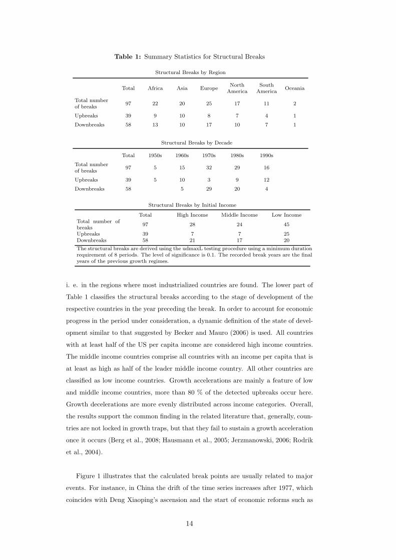
Table 1: Summary Statistics for Structural Breaks
Structural Breaks by Region
Total Africa Asia EuropeNorth
AmericaSouth
AmericaOceania
Total numberof breaks
97 22 20 25 17 11 2
Upbreaks 39 9 10 8 7 4 1
Downbreaks 58 13 10 17 10 7 1
Structural Breaks by Decade
Total 1950s 1960s 1970s 1980s 1990s
Total numberof breaks
97 5 15 32 29 16
Upbreaks 39 5 10 3 9 12
Downbreaks 58 5 29 20 4
Structural Breaks by Initial Income
Total High Income Middle Income Low IncomeTotal number ofbreaks
97 28 24 45
Upbreaks 39 7 7 25Downbreaks 58 21 17 20
The structural breaks are derived using the udmaxL testing procedure using a minimum durationrequirement of 8 periods. The level of significance is 0.1. The recorded break years are the finalyears of the previous growth regimes.
i. e. in the regions where most industrialized countries are found. The lower part of
Table 1 classifies the structural breaks according to the stage of development of the
respective countries in the year preceding the break. In order to account for economic
progress in the period under consideration, a dynamic definition of the state of devel-
opment similar to that suggested by Becker and Mauro (2006) is used. All countries
with at least half of the US per capita income are considered high income countries.
The middle income countries comprise all countries with an income per capita that is
at least as high as half of the leader middle income country. All other countries are
classified as low income countries. Growth accelerations are mainly a feature of low
and middle income countries, more than 80 % of the detected upbreaks occur here.
Growth decelerations are more evenly distributed across income categories. Overall,
the results support the common finding in the related literature that, generally, coun-
tries are not locked in growth traps, but that they fail to sustain a growth acceleration
once it occurs (Berg et al., 2008; Hausmann et al., 2005; Jerzmanowski, 2006; Rodrik
et al., 2004).
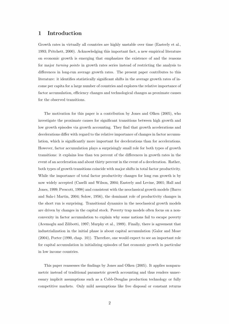
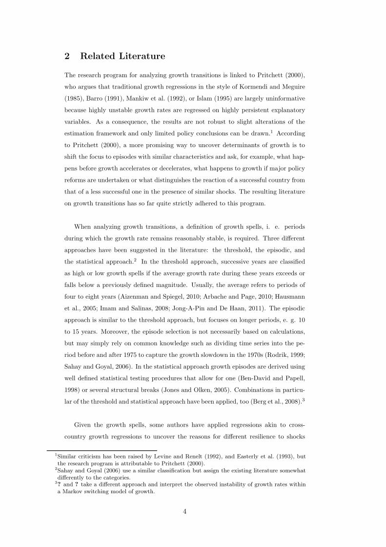
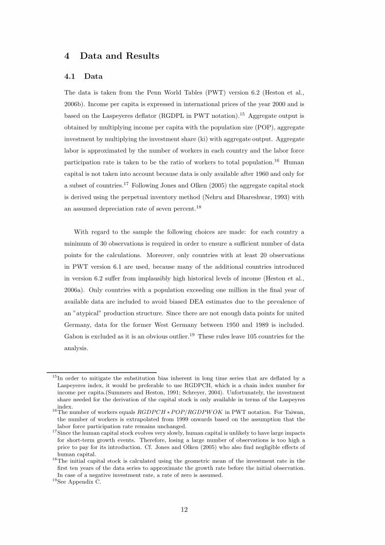
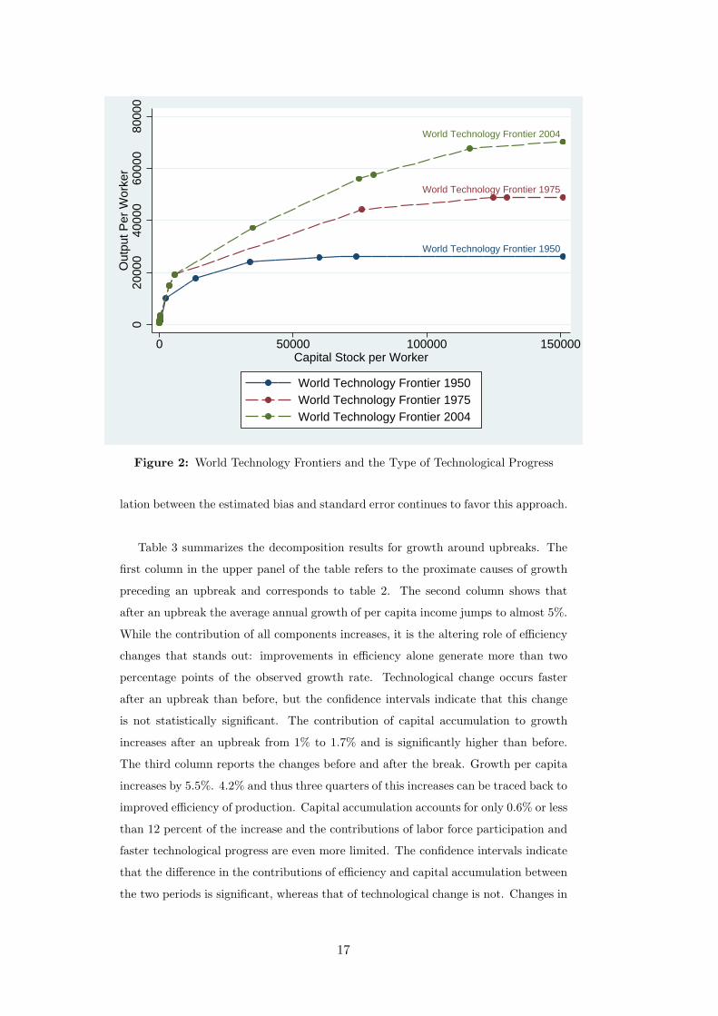
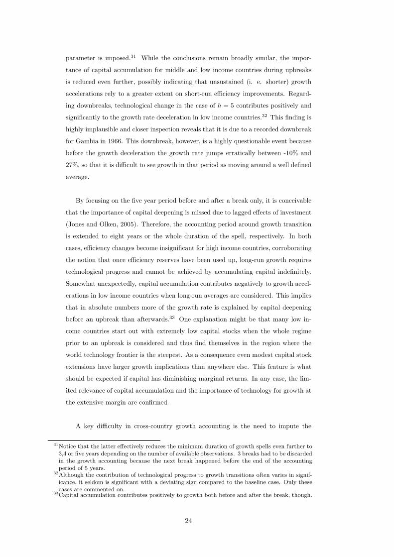
Figure 1 illustrates that the calculated break points are usually related to major
events. For instance, in China the drift of the time series increases after 1977, which
coincides with Deng Xiaoping’s ascension and the start of economic reforms such as
14
66.
57
7.5
88.
5Lo
g of
Inco
me
Per
Cap
ita
1950 1960 1970 1980 1990 2000Year
China
88.
59
Log
of In
com
e P
er C
apita
1950 1960 1970 1980 1990 2000Year
Mexico7.
58
8.5
99.
510
Log
of In
com
e P
er C
apita
1950 1960 1970 1980 1990 2000Year
Portugal
8.2
8.4
8.6
8.8
99.
2lo
g of
PP
P p
er−
capi
ta in
com
e
1970 1980 1990 2000 2010Year
Poland
Figure 1: Examples of Structural Breaks
the liberalization of agriculture and the opening of the economy. In Mexico, the de-
celeration of growth after 1981 can be linked to the severe currency crisis starting in
that year whereas the deceleration after 1973 in Portugal heralds the turbulent time
after a bloodless military coup. In Poland, the first turning point 1978 coincides with
the beginnings of the Solidarnosc Movement and severe price increases, whereas the
upbreak after 1991 can be related to the economic and political reforms after the fall of
communism. Poland also illustrates the trade-off introduced by imposing a minimum
duration requirement for each regime: the method identifies well defined break points,
but misses short-lived events that are very close to each other. In the case of Poland,
the growth acceleration between 1982 and 1988 is not picked up.
4.3 Proximate Causes of Growth Transitions
In order to account for the sources of growth transitions, nonparametric growth ac-
counting is carried out for the five year period before and for the five year period after
each break.25 The reported yearly contributions of capital accumulation, efficiency
change and technological change to yearly economic growth is the geometric average
25If the break year is, say, 1960, the regime before the break comprises g56, ..., g60 and the regimeafter the break comprises g61, ..., g65. g56 denotes the growth rate from 1955 to 1956.
15
of the corresponding numbers for the five year period.26 For ease of comparison with
traditional growth accounting studies, the results are presented as growth rates, so
that slight rounding errors owing to the conversion from growth factors to rates may
occur. Across countries arithmetic means means are reported.27 Before proceeding
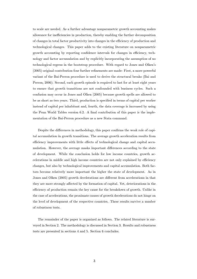
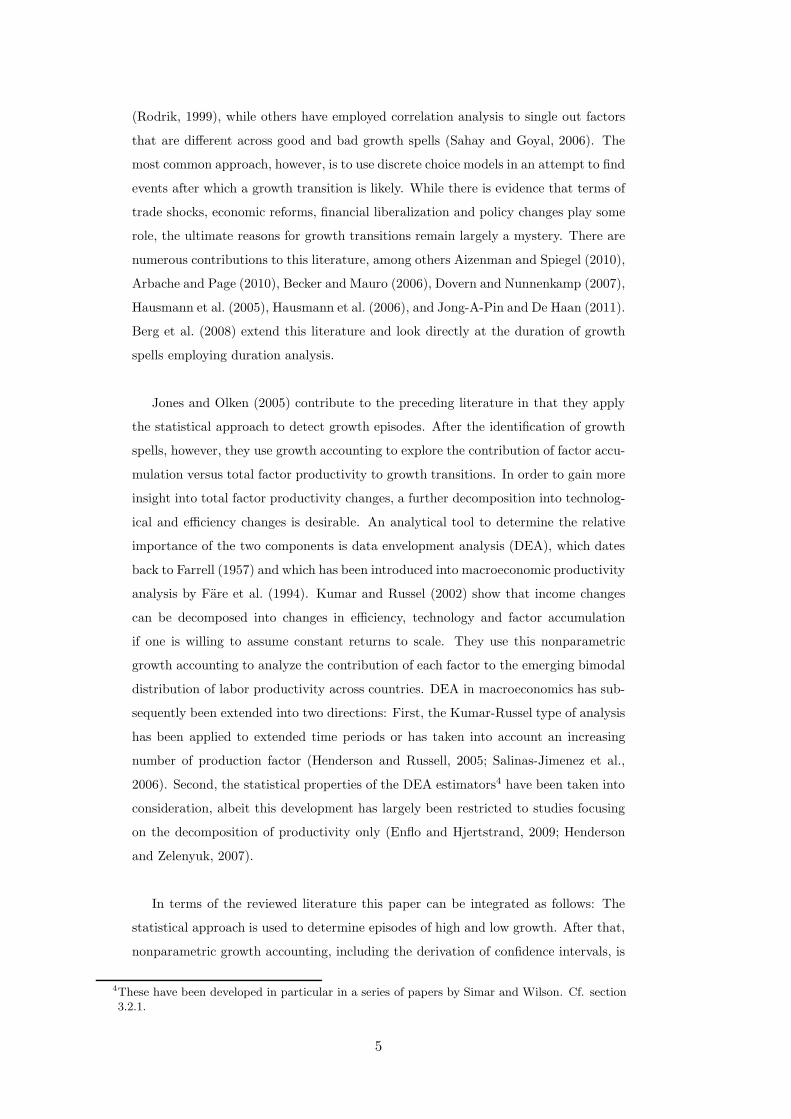
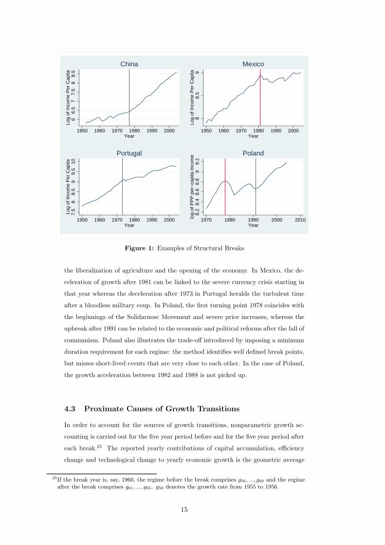
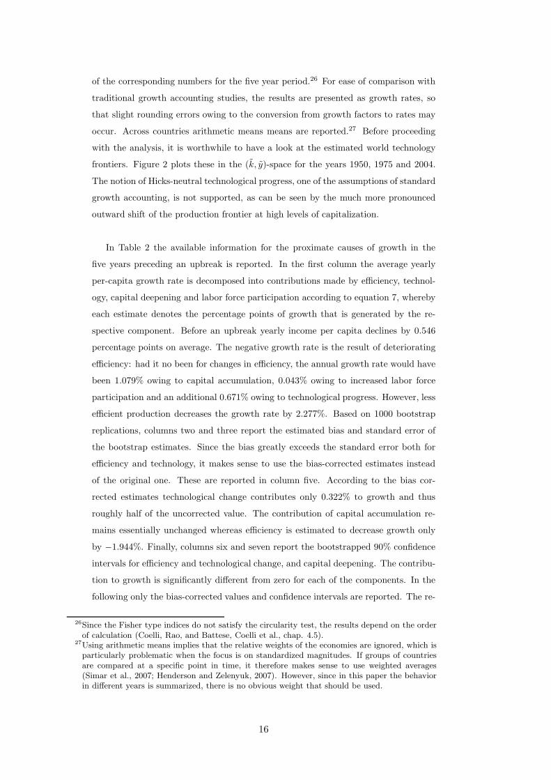
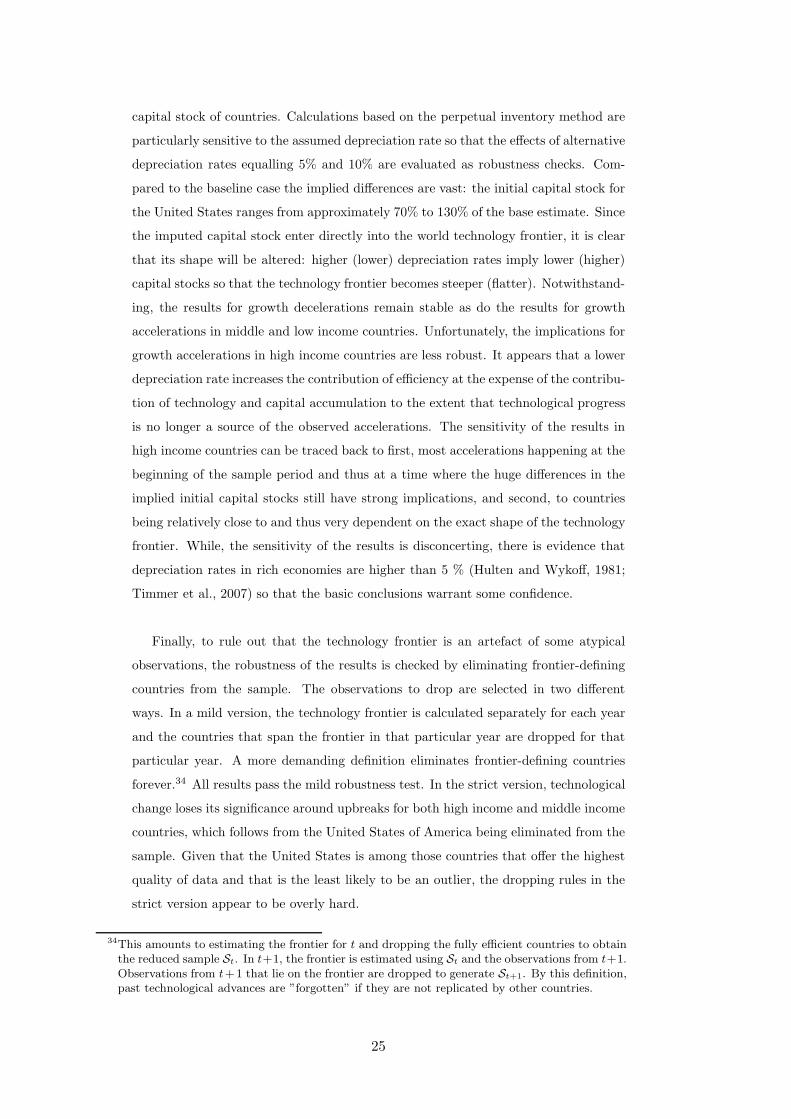
with the analysis, it is worthwhile to have a look at the estimated world technology
frontiers. Figure 2 plots these in the (k, y)-space for the years 1950, 1975 and 2004.
The notion of Hicks-neutral technological progress, one of the assumptions of standard
growth accounting, is not supported, as can be seen by the much more pronounced
outward shift of the production frontier at high levels of capitalization.
In Table 2 the available information for the proximate causes of growth in the
five years preceding an upbreak is reported. In the first column the average yearly
per-capita growth rate is decomposed into contributions made by efficiency, technol-
ogy, capital deepening and labor force participation according to equation 7, whereby
each estimate denotes the percentage points of growth that is generated by the re-
spective component. Before an upbreak yearly income per capita declines by 0.546
percentage points on average. The negative growth rate is the result of deteriorating
efficiency: had it no been for changes in efficiency, the annual growth rate would have
been 1.079% owing to capital accumulation, 0.043% owing to increased labor force
participation and an additional 0.671% owing to technological progress. However, less
efficient production decreases the growth rate by 2.277%. Based on 1000 bootstrap
replications, columns two and three report the estimated bias and standard error of
the bootstrap estimates. Since the bias greatly exceeds the standard error both for
efficiency and technology, it makes sense to use the bias-corrected estimates instead
of the original one. These are reported in column five. According to the bias cor-
rected estimates technological change contributes only 0.322% to growth and thus
roughly half of the uncorrected value. The contribution of capital accumulation re-
mains essentially unchanged whereas efficiency is estimated to decrease growth only
by −1.944%. Finally, columns six and seven report the bootstrapped 90% confidence
intervals for efficiency and technological change, and capital deepening. The contribu-
tion to growth is significantly different from zero for each of the components. In the
following only the bias-corrected values and confidence intervals are reported. The re-
26Since the Fisher type indices do not satisfy the circularity test, the results depend on the orderof calculation (Coelli, Rao, and Battese, Coelli et al., chap. 4.5).
27Using arithmetic means implies that the relative weights of the economies are ignored, which isparticularly problematic when the focus is on standardized magnitudes. If groups of countriesare compared at a specific point in time, it therefore makes sense to use weighted averages(Simar et al., 2007; Henderson and Zelenyuk, 2007). However, since in this paper the behaviorin different years is summarized, there is no obvious weight that should be used.
16
World Technology Frontier 1950
World Technology Frontier 1975
World Technology Frontier 20040
2000
040
000
6000
080
000
Out
put P
er W
orke
r
0 50000 100000 150000Capital Stock per Worker
World Technology Frontier 1950World Technology Frontier 1975World Technology Frontier 2004
Figure 2: World Technology Frontiers and the Type of Technological Progress
lation between the estimated bias and standard error continues to favor this approach.
Table 3 summarizes the decomposition results for growth around upbreaks. The
first column in the upper panel of the table refers to the proximate causes of growth
preceding an upbreak and corresponds to table 2. The second column shows that
after an upbreak the average annual growth of per capita income jumps to almost 5%.
While the contribution of all components increases, it is the altering role of efficiency
changes that stands out: improvements in efficiency alone generate more than two
percentage points of the observed growth rate. Technological change occurs faster
after an upbreak than before, but the confidence intervals indicate that this change
is not statistically significant. The contribution of capital accumulation to growth
increases after an upbreak from 1% to 1.7% and is significantly higher than before.
The third column reports the changes before and after the break. Growth per capita
increases by 5.5%. 4.2% and thus three quarters of this increases can be traced back to
improved efficiency of production. Capital accumulation accounts for only 0.6% or less
than 12 percent of the increase and the contributions of labor force participation and
faster technological progress are even more limited. The confidence intervals indicate
that the difference in the contributions of efficiency and capital accumulation between
the two periods is significant, whereas that of technological change is not. Changes in
17
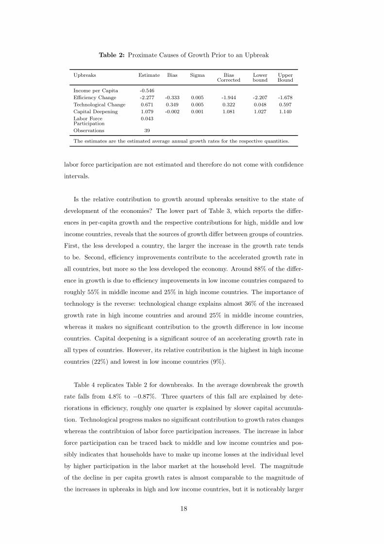
Table 2: Proximate Causes of Growth Prior to an Upbreak
Upbreaks Estimate Bias Sigma BiasCorrected
Lowerbound
UpperBound
Income per Capita -0.546
Efficiency Change -2.277 -0.333 0.005 -1.944 -2.207 -1.678
Technological Change 0.671 0.349 0.005 0.322 0.048 0.597
Capital Deepening 1.079 -0.002 0.001 1.081 1.027 1.140
Labor ForceParticipation
0.043
Observations 39
The estimates are the estimated average annual growth rates for the respective quantities.
labor force participation are not estimated and therefore do not come with confidence
intervals.
Is the relative contribution to growth around upbreaks sensitive to the state of
development of the economies? The lower part of Table 3, which reports the differ-
ences in per-capita growth and the respective contributions for high, middle and low
income countries, reveals that the sources of growth differ between groups of countries.
First, the less developed a country, the larger the increase in the growth rate tends
to be. Second, efficiency improvements contribute to the accelerated growth rate in
all countries, but more so the less developed the economy. Around 88% of the differ-
ence in growth is due to efficiency improvements in low income countries compared to
roughly 55% in middle income and 25% in high income countries. The importance of
technology is the reverse: technological change explains almost 36% of the increased
growth rate in high income countries and around 25% in middle income countries,
whereas it makes no significant contribution to the growth difference in low income
countries. Capital deepening is a significant source of an accelerating growth rate in
all types of countries. However, its relative contribution is the highest in high income
countries (22%) and lowest in low income countries (9%).
Table 4 replicates Table 2 for downbreaks. In the average downbreak the growth
rate falls from 4.8% to −0.87%. Three quarters of this fall are explained by dete-
riorations in efficiency, roughly one quarter is explained by slower capital accumula-
tion. Technological progress makes no significant contribution to growth rates changes
whereas the contribtuion of labor force participation increases. The increase in labor
force participation can be traced back to middle and low income countries and pos-
sibly indicates that households have to make up income losses at the individual level
by higher participation in the labor market at the household level. The magnitude
of the decline in per capita growth rates is almost comparable to the magnitude of
the increases in upbreaks in high and low income countries, but it is noticeably larger
18
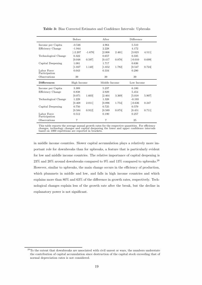
Table 3: Bias Corrected Estimates and Confidence Intervals: Upbreaks
Before After Difference
Income per Capita -0.546 4.964 5.510
Efficiency Change -1.944 2.228 4.172
[-2.207 -1.678] [2.008 2.461] [3.823 4.511]
Technological Change 0.322 0.657 0.335
[0.048 0.597] [0.417 0.878] [-0.010 0.699]
Capital Deepening 1.081 1.717 0.636
[1.027 1.140] [1.652 1.782] [0.547 0.724]
Labor ForceParticipation
0.043 0.334 0.290
Observations 39 39 39
Differences High Income Middle Income Low Income
Income per Capita 3.389 5.237 6.180
Efficiency Change 0.838 2.929 5.454
[0.071 1.603] [2.464 3.369] [5.018 5.907]
Technological Change 1.229 1.328 -0.193
[0.468 2.011] [0.896 1.754] [-0.636 0.247
Capital Deepening 0.750 0.725 0.579
[0.584 0.912] [0.589 0.874] [0.451 0.711]
Labor ForceParticipation
0.512 0.190 0.257
Observations 7 7 25
This table reports the average annual growth rates for the respective quantities. For efficiencychanges, technology changes and capital deepening the lower and upper confidence intervalsbased on 1000 repetitions are reported in brackets.
in middle income countries. Slower capital accumulation plays a relatively more im-
portant role for downbreaks than for upbreaks, a feature that is particularly evident
for low and middle income countries. The relative importance of capital deepening is
23% and 20% around downbreaks compared to 9% and 13% compared to upbreaks.28
However, similar to upbreaks, the main change occurs in the efficiency of production,
which plummets in middle and low, and falls in high income countries and which
explains more than 80% and 63% of the difference in growth rates, respectively. Tech-
nological changes explain less of the growth rate after the break, but the decline in
explanatory power is not significant.
28To the extent that downbreaks are associated with civil unrest or wars, the numbers understatethe contribution of capital accumulation since destruction of the capital stock exceeding that ofnormal depreciation rates is not considered.
19
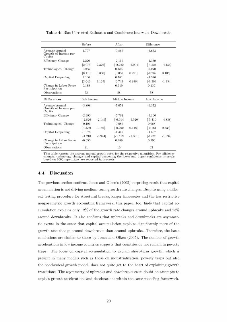
Table 4: Bias Corrected Estimates and Confidence Intervals: Downbreaks
Before After Difference
Average AnnualGrowth of Income perCapita
4.797 -0.867 -5.663
Efficiency Change 2.220 -2.119 -4.339
[2.076 2.376] [-2.222 -2.004] [-4.524 -4.156]
Technological Change 0.255 0.185 -0.070
[0.119 0.380] [0.068 0.291] [-0.232 0.105]
Capital Deepening 2.106 0.781 -1.326
[2.046 2.165] [0.742 0.818] [-1.394 -1.254]
Change in Labor ForceParticipation
0.188 0.319 0.130
Observations 58 58 58
Differences High Income Middle Income Low Income
Average AnnualGrowth of Income perCapita
-3.898 -7.051 -6.372
Efficiency Change -2.490 -5.761 -5.106
[-2.826 -2.149] [-6.014 -5.520] [-5.410 -4.838]
Technological Change -0.196 -0.086 0.068
[-0.549 0.146] [-0.290 0.118] [-0.181 0.335]
Capital Deepening -1.076 -1.415 -1.507
[-1.210 -0.944] [-1.519 -1.301] [-1.623 -1.394]
Change in Labor ForceParticipation
-0.050 0.289 0.190
Observations 21 16 21
This table reports the average annual growth rates for the respective quantities. For efficiencychanges, technology changes and capital deepening the lower and upper confidence intervalsbased on 1000 repetitions are reported in brackets.
4.4 Discussion
The previous section confirms Jones and Olken‘s (2005) surprising result that capital
accumulation is not driving medium-term growth rate changes. Despite using a differ-
ent testing procedure for structural breaks, longer time-series and the less restrictive
nonparametric growth accounting framework, this paper, too, finds that capital ac-
cumulation explains only 12% of the growth rate changes around upbreaks and 23%
around downbreaks. It also confirms that upbreaks and downbreaks are asymmet-
ric events in the sense that capital accumulation explains significantly more of the
growth rate change around downbreaks than around upbreaks. Therefore, the basic
conclusions are similar to those by Jones and Olken (2005). The number of growth
accelerations in low income countries suggests that countries do not remain in poverty
traps. The focus on capital accumulation to explain short-term growth, which is
present in many models such as those on industrialization, poverty traps but also
the neoclassical growth model, does not quite get to the heart of explaining growth
transitions. The asymmetry of upbreaks and downbreaks casts doubt on attempts to
explain growth accelerations and decelerations within the same modeling framework.
20
The decomposition of productivity changes into efficiency changes and changes in
technology and the distinction of countries according to their state of development
offers further insights. Based on the numbers for total averages only, technological
improvements seem unimportant in the context of medium-term growth rate changes.
Changes in total factor productivity appear to reflect almost entirely changes in the
efficiency of production. However, a different assessment follows if growth accelera-
tions are analyzed according to the state of development of the respective countries at
the timing of the breaks. Whereas technological improvements are indeed irrelevant
for low income countries, this does not hold for middle and high income countries.
These countries benefit from technological progress around upbreaks and it is quite
possible that the enhanced production possibilities gained by technological improve-
ments are the ultimate reason behind the accelerated growth rate. The fact that the
contribution of capital accumulation to accelerations of the growth rate increases with
technological improvements may further indicate that technological progress is of the
embodied type. Hence, the endogenous growth framework with embodied technologi-
cal progress may be a promising modeling framework for these countries and may be
very informative at suggesting appropriate policies to achieve growth accelerations.
Clearly, the driving forces of growth accelerations are very different for the less
developed countries. Growth accelerations in this country group are essentially im-
provements in the efficiency of production with not much else going on. Hence, the
reallocation of resources appears to be a central element of what is happening. How
this reallocation is achieved is an open question and should be the focus of future
studies. Jones and Olken (2005) suggest that openness and the composition of manu-
facturing are essential. Yet, these kind of changes are not sufficient to predict growth
accelerations (Hausmann et al., 2005), so that more encompassing explanations are
required. The literature also acknowledges that initiating growth accelerations is dif-
ferent from sustaining them (Rodrik, 2005). The present framework points at one
possible reason. If low income countries initially grow on the intensive margin by
improving the efficiency of production, at some point these benefits will be reaped
and the countries will have to switch to the extensive margin and either accumulate
capital or innovate. It is conceivable that the inability of many poor countries to
sustain growth accelerations is a consequence of the countries’ failure to undergo this
change.
Downbreaks differ from upbreaks in two respects: first, less rapid capital accumula-
tion is a non-negligible part of the explanation and second, massive falls of productive
efficiency occur across all country groups. However, the decrease of efficiency might
21
be overstated. The calculations are based on per worker values, which themselves are
constructed using labor force participation rates that do not account for unemploy-
ment or hours worked. Therefore, if unemployment during downbreaks increases or if
hours worked fall, output per worker and hence efficiency is underestimated.29 Still,
the direction of the potential error is not unequivocal because the same argument im-
plies that capital per worker is understated or lies idle, which leads to overestimated
efficiency scores. Obviously, a better way to account for capacity utilization is desir-
able, but it is quite likely that efficiency changes will continue to play a major role.30
The reasons for the observed decline in efficiency are of major interest and should be
the focus of additional research. Based on the existing literature, conceivable expla-
nations include civil conflict, bad macroeconomic management (e.g. hyper inflation),
adverse terms of trade shocks coupled with an inflexible production structure, price
shocks, inflexibility due to vested interest group or demography to name just a few
(Hausmann et al., 2006; Feyrer, 2009; Funke et al., 2008; Becker and Mauro, 2006).
Since many of these aspects are difficult to measure, the most rewarding way forward
appears to be a series of case studies to find out the common factors present in all
countries.
5 Robustness Checks
Due to the well known sensitivity of DEA analysis to atypical observations, the previ-
ous results have to be checked for robustness. This section analyzes the consequences
of altering the assumptions used in the BP procedure and the derivation of the capital
stock, of extending the accounting period around growth transitions and of eliminating
frontier-defining countries from the sample. Table 5 shows how the contributions of
efficiency, technology and capital deepening change across growth transitions in high,
middle and low income countries. The bias-correction of the estimates is based on 200
bootstrap replications.
Consider the robustness with regard to the BP assumptions first. The structural
breaks are derived using heteroscedasticity and autocorrelation consistent standard
errors, a minimum duration requirement of five years or a constant trimming pa-
rameter of 0.1, respectively. HAC standard errors imply additional breaks, but do not
significantly influence the conclusions otherwise. The number of break points is also in-
creased if the minimum duration of growth spells is reduced or if a constant trimming
29However, it might be argued that unemployment should be considered in the efficiency on aneconomy-wide level.
30Jones and Olken (2005) employ electricity consumption to assess capacity utilization more di-rectly. Their results are not sensitive to this change.
22
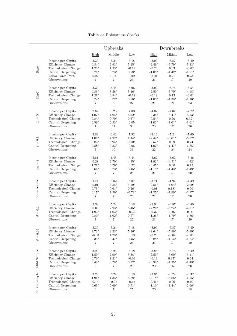
Table 5: Robustness Checks
Upbreaks Downbreaks
High Middle Low High Middle Low
Base
Income per Capita 3.39 5.24 6.18 -3.90 -6.87 -6.49Efficiency Change 0.84∗ 2.93∗ 5.45∗ -2.49∗ -5.70∗ -5.13∗
Technological Change 1.23∗ 1.33∗ -0.19 -0.20 0.03 -0.02Capital Deepening 0.75∗ 0.73∗ 0.58∗ -1.08∗ -1.42∗ -1.51∗
Labor Force Part. 0.22 0.14 0.09 0.28 0.21 0.23Observations 7 7 25 21 17 20
HAC
Income per Capita 3.39 5.44 5.96 -3.90 -6.75 -6.54Efficiency Change 0.86∗ 3.38∗ 5.16∗ -2.50∗ -5.70∗ -4.98∗
Technological Change 1.21∗ 0.94∗ -0.18 -0.18 0.13 -0.01Capital Deepening 0.74∗ 0.77∗ 0.66∗ -1.08∗ -1.38∗ -1.76∗
Observations 7 8 27 21 18 23
h=
5
Income per Capita 2.82 6.23 7.00 -4.02 -7.07 -7.72Efficiency Change 1.07∗ 4.95∗ 6.02∗ -2.35∗ -6.41∗ -6.53∗
Technological Change 0.84∗ 0.70∗ 0.67∗ -0.54∗ 0.20 0.32∗
Capital Deepening 0.59∗ 0.33∗ 0.05 -1.02∗ -1.01∗ -1.61∗
Observations 7 11 30 23 17 26
ε=
0.1
Income per Capita 2.82 6.42 7.92 -4.16 -7.24 -7.60Efficiency Change 1.09∗ 4.92∗ 7.14∗ -2.44∗ -6.01∗ -6.07∗
Technological Change 0.83∗ 0.95∗ 0.60∗ -0.57∗ 0.09 0.24Capital Deepening 0.58∗ 0.33∗ 0.06 -1.02∗ -1.47∗ -1.85∗
Observations 7 10 33 22 16 24
acc=
8
Income per Capita 2.81 4.45 5.44 -3.62 -5.62 -5.46Efficiency Change 0.28 2.70∗ 4.35∗ -1.92∗ -4.51∗ -4.32∗
Technological Change 1.21∗ 0.76∗ 0.22 -0.45∗ 0.00 0.13Capital Deepening 0.66∗ 0.73∗ 0.45∗ -1.19∗ -1.43∗ -1.48∗
Observations 7 7 25 21 17 20
acc=
regim
e Income per Capita 1.74 5.82 5.07 -3.71 -4.94 -4.49Efficiency Change 0.01 3.55∗ 4.79∗ -2.51∗ -4.04∗ -2.09∗
Technological Change 0.75∗ 0.61∗ 0.26∗ -0.01 0.18∗ 0.09Capital Deepening 0.17∗ 1.20∗ -0.72∗ -1.25∗ -1.99∗ -2.97∗
Observations 7 7 25 21 17 20
δ=
0.1
Income per Capita 3.39 5.24 6.18 -3.90 -6.87 -6.49Efficiency Change 0.09 2.93∗ 5.45∗ -2.20∗ -5.24∗ -4.81∗
Technological Change 1.93∗ 1.03∗ -0.39 -0.32 -0.07 0.00Capital Deepening 0.80∗ 1.02∗ 0.77∗ -1.26∗ -1.79∗ -1.86∗
Observations 7 7 25 21 17 20
δ=
0.05
Income per Capita 3.39 5.24 6.18 -3.90 -6.87 -6.49Efficiency Change 2.73∗ 3.23∗ 5.26∗ -2.64∗ -5.90∗ -5.40∗
Technological Change -0.33 1.28∗ 0.13 -0.23 -0.04 -0.01Capital Deepening 0.39∗ 0.47∗ 0.45∗ -0.88∗ -1.15∗ -1.24∗
Observations 7 7 25 21 17 20
MildSample Income per Capita 3.29 5.24 6.18 -3.85 -6.76 -6.49
Efficiency Change 1.59∗ 2.99∗ 5.38∗ -2.59∗ -6.00∗ -5.41∗
Technological Change 0.70∗ 1.21∗ -0.06 -0.13 0.35∗ 0.24Capital Deepening 0.48∗ 0.79∗ 0.52∗ -0.98∗ -1.35∗ -1.48∗
Observations 6 7 25 20 16 20
StrictSample Income per Capita 3.29 5.24 6.18 -3.85 -6.74 -6.32
Efficiency Change 1.96∗ 4.35∗ 5.28∗ -2.18∗ -5.66∗ -4.55∗
Technological Change 0.14 -0.07 -0.15 -0.41∗ 0.06 0.10Capital Deepening 0.65∗ 0.69∗ 0.71∗ -1.10∗ -1.44∗ -2.06∗
Observations 6 7 25 20 14 18
23
parameter is imposed.31 While the conclusions remain broadly similar, the impor-
tance of capital accumulation for middle and low income countries during upbreaks
is reduced even further, possibly indicating that unsustained (i. e. shorter) growth
accelerations rely to a greater extent on short-run efficiency improvements. Regard-
ing downbreaks, technological change in the case of h = 5 contributes positively and
significantly to the growth rate deceleration in low income countries.32 This finding is
highly implausible and closer inspection reveals that it is due to a recorded downbreak
for Gambia in 1966. This downbreak, however, is a highly questionable event because
before the growth deceleration the growth rate jumps erratically between -10% and
27%, so that it is difficult to see growth in that period as moving around a well defined
average.
By focusing on the five year period before and after a break only, it is conceivable
that the importance of capital deepening is missed due to lagged effects of investment
(Jones and Olken, 2005). Therefore, the accounting period around growth transition
is extended to eight years or the whole duration of the spell, respectively. In both
cases, efficiency changes become insignificant for high income countries, corroborating
the notion that once efficiency reserves have been used up, long-run growth requires
technological progress and cannot be achieved by accumulating capital indefinitely.
Somewhat unexpectedly, capital accumulation contributes negatively to growth accel-
erations in low income countries when long-run averages are considered. This implies
that in absolute numbers more of the growth rate is explained by capital deepening
before an upbreak than afterwards.33 One explanation might be that many low in-
come countries start out with extremely low capital stocks when the whole regime
prior to an upbreak is considered and thus find themselves in the region where the
world technology frontier is the steepest. As a consequence even modest capital stock
extensions have larger growth implications than anywhere else. This feature is what
should be expected if capital has diminishing marginal returns. In any case, the lim-
ited relevance of capital accumulation and the importance of technology for growth at
the extensive margin are confirmed.
A key difficulty in cross-country growth accounting is the need to impute the
31Notice that the latter effectively reduces the minimum duration of growth spells even further to3,4 or five years depending on the number of available observations. 3 breaks had to be discardedin the growth accounting because the next break happened before the end of the accountingperiod of 5 years.
32Although the contribution of technological progress to growth transitions often varies in signif-icance, it seldom is significant with a deviating sign compared to the baseline case. Only thesecases are commented on.
33Capital accumulation contributes positively to growth both before and after the break, though.
24
capital stock of countries. Calculations based on the perpetual inventory method are
particularly sensitive to the assumed depreciation rate so that the effects of alternative
depreciation rates equalling 5% and 10% are evaluated as robustness checks. Com-
pared to the baseline case the implied differences are vast: the initial capital stock for
the United States ranges from approximately 70% to 130% of the base estimate. Since
the imputed capital stock enter directly into the world technology frontier, it is clear
that its shape will be altered: higher (lower) depreciation rates imply lower (higher)
capital stocks so that the technology frontier becomes steeper (flatter). Notwithstand-
ing, the results for growth decelerations remain stable as do the results for growth
accelerations in middle and low income countries. Unfortunately, the implications for
growth accelerations in high income countries are less robust. It appears that a lower
depreciation rate increases the contribution of efficiency at the expense of the contribu-
tion of technology and capital accumulation to the extent that technological progress
is no longer a source of the observed accelerations. The sensitivity of the results in
high income countries can be traced back to first, most accelerations happening at the
beginning of the sample period and thus at a time where the huge differences in the
implied initial capital stocks still have strong implications, and second, to countries
being relatively close to and thus very dependent on the exact shape of the technology
frontier. While, the sensitivity of the results is disconcerting, there is evidence that
depreciation rates in rich economies are higher than 5 % (Hulten and Wykoff, 1981;
Timmer et al., 2007) so that the basic conclusions warrant some confidence.
Finally, to rule out that the technology frontier is an artefact of some atypical
observations, the robustness of the results is checked by eliminating frontier-defining
countries from the sample. The observations to drop are selected in two different
ways. In a mild version, the technology frontier is calculated separately for each year
and the countries that span the frontier in that particular year are dropped for that
particular year. A more demanding definition eliminates frontier-defining countries
forever.34 All results pass the mild robustness test. In the strict version, technological
change loses its significance around upbreaks for both high income and middle income
countries, which follows from the United States of America being eliminated from the
sample. Given that the United States is among those countries that offer the highest
quality of data and that is the least likely to be an outlier, the dropping rules in the
strict version appear to be overly hard.
34This amounts to estimating the frontier for t and dropping the fully efficient countries to obtainthe reduced sample St. In t+1, the frontier is estimated using St and the observations from t+1.Observations from t+1 that lie on the frontier are dropped to generate St+1. By this definition,past technological advances are ”forgotten” if they are not replicated by other countries.
25
Summing up, most results are robust to a variety of specification changes. In
particular, the limited importance of capital accumulation and the dominating role of
efficiency improvement for growth accelerations in middle and low income countries
is highly robust. The results for high income countries are somewhat more sensitive,
but there are good reasons to trust the findings that these countries benefit from
technological improvements and capital accumulation in growth accelerations. The
results for downbreaks are even more robust. Growth decelerations are explained by
lower contributions of capital accumulation and by huge efficiency deteriorations.
6 Conclusion
In this paper the proximate causes of significant growth rate changes within countries
have been analyzed with a special focus on the relative importance of factor accumu-
lation versus productivity changes in order to test the robustness of a recent finding
by Jones and Olken (2005): namely that total factor productivity improvements not
only drive long-term growth, but also short-term growth events. Methodologically,
nonparametric growth accounting has been applied because this helps to avoid a num-
ber of assumptions implicit in parametric growth accounting. Moreover, productivity
changes can be attributed to changes in efficiency and changes in technology.
Despite the tendency of nonparametric growth accounting to find an increased
role for factor accumulation compared to traditional growth accounting (Henderson
and Russell, 2005; Jerzmanowski, 2007) and despite the finding that the Hicks-neutral
technological progress assumption of parametric growth accounting is not justified,
the present study confirms that even short-run growth transitions are mainly produc-
tivity events. Depending on the level of development at least three quarters of growth
accelerations and decelerations are explained by efficiency and technological changes.
In contrast to predictions by neoclassical growth models, capital accumulation con-
tributes the most to growth rate increases in high income countries and the least
to those in low income countries. Growth accelerations in low income countries are
mainly due to improvements in the efficiency of production. Technological progress
benefits middle and high income, but not low income countries. Growth decelerations
are the result of slower capital accumulation and deteriorating efficiency levels. Unlike
before, the level of development has only minor impacts on the relative contributions
of the different drivers of growth. Finally, like Jones and Olken (2005) the present
study corroborates the view that growth accelerations are different from deceleration
in that the importance of capital accumulation is significantly higher in the latter.
26
These results are robust to a number of specification changes.
The most lasting impression of the accounting exercise is the dominance of effi-
ciency changes to explain growth transitions. Therefore, the next logical step is to
search for the sources of efficiency changes. The literature has identified a multitude
of factors that may influence the efficiency of production at the economy-wide level.
Among these are the sectoral composition of production, the skill composition in the
economy, the prevailing regulations and laws, the organization of vested interests, the
integration into the world economy and thereby the ability to benefit from spillovers
or scale economies, the prevalence of violent conflicts and rent-seeking, the availability
of a well-functioning financial system or a reasonable level of trust between market
participants to name just a few (Acemoglu and Zilibotti, 2001; Edwards, 1993; Frankel
and Romer, 1999; ?; ?; ?; Murphy et al., 1989; Prescott, 1998). It is an open question
whether there are typical patterns which countries experiencing significant and lasting
efficiency changes have in common thus lending themselves to become blueprints of
reforms or whether changes are country-specific and not easily transferable (Rodrik,
2005; Williamson, 1990). Most likely, a fruitful analysis will require more detailed
data on economic reforms and institutional changes than are currently available. It
might also be beneficial to focus directly on breaks in the efficiency scores rather than
choosing the indirect way using growth transitions. In any case, a more thorough un-
derstanding of the mechanisms that determine the efficiency of production is needed
to understand the forces holding back countries from prosperity.
References
Acemoglu, D. and D. Autor (2010). Skills, Tasks and Technologies: Implications for
Employment and Earnings. NBER Working Paper 16082 .
Acemoglu, D. and F. Zilibotti (1997). Was Prometheus Unbound by Chance? Risk,
Diversification, and Growth. Journal of Political Economy 105, 709–751.
Acemoglu, D. and F. Zilibotti (2001). Productivity Differences. Quarterly Journal of
Economics 116, 563–606.
Aizenman, J. and M. Spiegel (2010). Takeoffs. Review of Development Economics 14,
177–196.
Andrews, D. W. K. (1991). Heteroskedasticity and Autocorrelation Consistent Co-
variance Matrix Estimation. Econometrica 59, 817–858.
27
Andrews, D. W. K. and J. C. Monahan (1992). An Improved Heteroscedasticity and
Autocorrelation Consistent Covariance Matrix Estimator. Econometrica 60, 953–
966.
Arbache, J. S. and J. Page (2010). How Fragile is Africa’s Recent Growth? Journal
of African Economies 19, 1–24.
Bai, J. and P. Perron (1998). Estimating and Testing Linear Models with Multiple
Structural Changes. Econometrica 66, 47–78.
Bai, J. and P. Perron (2003a). Computation and Analysis of Multiple Structural
Change Models. Journal of Applied Econometrics 18, 1–22.
Bai, J. and P. Perron (2003b). Critical Values for Multiple Structural Change Tests.
Econometrics Journal 6, 72–78.
Bai, J. and P. Perron (2006). Multiple Structural Change Models: A Simulation
Analysis. pp. 212 – 240. Cambridge University Press.
Barro, R. J. (1991). Economic Growth in a Cross Section of Countries. Quarterly
Journal of Economics 106, 407–443.
Barro, R. J. and X. Sala-i Martin (2004). Economic Growth. MIT Press.
Becker, T. and P. Mauro (2006). Output Drops, and the Shocks that Matter. IMF
Working Paper 06/172 .
Ben-David, D. and D. H. Papell (1998). Slowdowns and Meltdowns: Postwar Growth
Evidences From 74 Countries. Review of Economics and Statistics 0, 561–571.
Bentolila, S. and G. Saint-Paul (2003). Explaining Movements in the Labor Share.
The B. E. Journal of Macroeconomics 3, xxxx.
Berg, A., C. Leite, and J. D. a. Ostry (2008). What Makes Growth Sustained? In-
ternational Monetary Fund Working Paper 08/59 .
Brown, R. L., J. Durbin, and M. Evans (1975). Techniques for Testing the Constancy
of Regression Relationships over Time. Journal of the Royal Statistical Society,
Series B 37, 149–192.
Caselli, F. and D. J. Wilson (2004). Importing technology. Journal of Monetary
Economics 51, 1–32.
Caves, D. W., L. R. Christensen, and E. W. Diewert (1982). The Economic The-
ory of Index Numbers and the Measurement of Input, Output and Productivity.
Econometrica 50, 1393–1414.
28
Coelli, T., D. S. P. Rao, and G. E. Battese. An Introduction to Efficiency and Pro-
ductivity Analysis. Kluwer Academic Publishers.
Crafts, N. F. R. (2003). Quantifying the Contribution of Technological Change to
Economic Growth in Different Eras: A Review of Evidence. London School of
Economics 79/03.
Dovern, J. and P. Nunnenkamp (2007). Aid and Growth Accelerations: An Alternative
Approach to Assessing the Effectiveness of Aid. Kyklos 60, 359–383.
Duffy, J. and C. Papageorgiou (2000). A Cross-Country Empirical Investigation of
the Aggregate Production Function Specification. Journal of Economic Growth 5,
87–120.
Easterly, W., M. Kremer, L. Pritchett, and L. H. Summers (1993). Good Policy or
Good Luck? Country Growth Performance and Temporary Shocks. Journal of
Monetary Economics 32, 459–483.
Easterly, W. and R. Levine (2001). It’s Not Factor Accumulation: Stylized Facts and
Growth Models. The World Bank Economic Review 15, 177–219.
Edwards, S. (1993). Openness, Trade Liberalization, and Growth in Developing Coun-
tries. Journal of Economic Literature 31, 1358–1393.
Enflo, K. and P. Hjertstrand (2009). Relative Sources of European Regional Produc-
tivity Convergence: A Bootstrap Frontier Approach. Regional Studies 43, 643–659.
Farrell, M. (1957). The Measurement of Productive Efficiency. Journal of the Royal
Statistical Society. Series A (General) 120, 253–290.
Felipe, J. and F. M. Fisher (2003). Aggregation in Production Functions: What
Applied Economists Should Know. Metroeconomica 54, 208–262.
Feyrer, J. (2009). The US Productivity Slowdown, the Baby Boom, and Management
Quality. NBER Working Paper 15474 .
Frankel, J. A. and D. Romer (1999). Does Trade Cause Growth? American Economic
Review 89, 379–399.
Fare, R., S. Grosskopf, and M. Norris (1994). Productivity Growth, Technical
Progress, and Efficiency Change in Industrialized Countries. American Economic
Review 84, 66–83.
Funke, N., E. Granziera, and P. Imam (2008). Terms of Trade Shocks in Economic
Recovery. WP/08/36.
29
Galor, O. and O. Moav (2004). From Physical to Human Capital Accumulation:
Inequality and the Process of Development. Review of Economic Studies 71, 1001–
1026.
Gollin, D. (2002). Getting Income Shares Right. Journal of Political Economy 110,
458–474.
Greene, W. H. (2003). Econometric Analysis. Pearson Education International.
Hall, R. and C. I. Jones (1999). Why Do Some Countries Produce So Much More
Output per Worker than Others? Quarterly Journal of Economics 114, 83–116.
Hausmann, R., L. Pritchett, and D. Rodrik (2005). Growth Accelerations. Journal of
Economic Growth 10, 303–329.
Hausmann, R., F. Rodriguez, and R. Wagner (2006). Growth Collapses. KSG Working
Paper RWP06-046.
Henderson, D. J. and R. R. Russell (2005). Human Capital and Convergence: A
Production-Frontier Approach. International Economic Review 46, 1167–1205.
Henderson, D. J. and V. Zelenyuk (2007). Testing for (Efficiency) Catching-up. South-
ern Economic Journal 73, 1003–1019.
Heston, A., R. Summers, and B. Aten (2006a). About PWT 6.2. Center for Interna-
tional Comparisons of Production.
Heston, A., R. Summers, and B. Aten (2006b). Penn World Table Version 6.2. Center
for International Comparisons of Production.
Hulten, C. R. and F. C. Wykoff (1981). The Measurement of Economic Depreciation.
pp. 81–125. Urban Institute.
Imam, P. and G. Salinas (2008). Explaining Episodes of Growth Accelerations, De-
celerations, and Collapses in Western Africa. IMF Working Paper 08/287 .
Islam, N. (1995). Growth Empirics: A Panel Data Approach. Quarterly Journal of
Economics 110, 1127–1170.
Jerzmanowski, M. (2006). Empirics of Hills, Plateaus, Mountains and Plains: A
Markov-Switching Approach to Growth. Journal of Development Economics 81,
357–385.
Jerzmanowski, M. (2007). Total Factor Productivity Differences: Appropriate Tech-
nology vs. Efficiency. European Economic Review 51, 2080–2110.
30
Jones, B. F. and B. A. Olken (2005). The Anatomy of Start-Stop Growth. NBER
Working Paper 11528.
Jong-A-Pin, R. and J. De Haan (2011). Political Regime Change, Economic Reform
and Growth Accelerations. Public Choice 146, 93–115.
Kejriwal, M. and P. Perron (2010). A Sequential Procedure to Determine the Number
of Breaks in Trend with an Integrated or Stationary Noise Components. Journal of
Time Series Analysis 31, 305–328.
Kormendi, R. C. and P. G. Meguire (1985). Macroeconomic Determinants of Growth:
Cross-Country Evidence. Journal of Monetary Economics 16, 141–163.
Krueger, A. B. (1999). Measuring Labor’s Share. American Economic Review Papers
And Procedings 89, 45–51.
Kumar, S. and R. R. Russel (2002). Technological Change, Technological Catch-
up, and Capital Deepening: Relative Contributions to Growth and Convergence.
American Economic Review 92, 527–548.
Kumbhakar, S. C. and C. A. K. Lovell (2000). Stochastic Frontier Analysis. Cambridge
University Press.
Levine, R. and D. Renelt (1992). A Sensitivity Analysis of Cross-Country Growth
Regressions. American Economic Review 82, 942–963.
Mankiw, G. N., D. Romer, and D. N. Weil (1992). A Contribution to the Empirics of
Economic Growth. Quarterly Journal of Economics 107, 407 – 437.
Murphy, K. M., A. Shleifer, and R. Vishny (1989). Income Distribution, Market Size
and Industrialization. Quarterly Journal of Economics 0, 537–564.
Nehru, V. and A. Dhareshwar (1993). A New Database on Physical Capital Stock:
Sources, Methodology and Results. Revista de Analisis Economico 8, 37–59.
Nelson, R. (1973). Recent Exercises in Growth Accounting: New Understanding or
Dead End? American Economic Review 63, 462–468.
Porter, M. E. (1990). The Competitive Advantage of Nations. Free Press.
Prescott, E. (1998). Needed: A Theory of Total Factor Productivity. International
Economic Review 39, 525–552.
Pritchett, L. (2000). Understanding Patterns of Economic Growth: Searching for Hills
among Plateaus, Mountains, and Plains. The World Bank Economic Review 14,
221–250.
31
Ray, S. C. (2004). Data Envelopment Analysis - Theory and Techniques for Economics
and Operations Research. Cambridge University Press.
Rodrik, D. (1997). TFPG Controversies, Institutions, and Economic Performance in
East Asia. NBER Working Paper Series 5914.
Rodrik, D. (1999). Where Did All the Growth Go? External Shocks, Social Conflict
and Growth Collapses. Journal of Economic Growth 4, 385–412.
Rodrik, D. (2005). Growth Strategies. pp. 967–1014.
Rodrik, D., A. Subramanian, and F. Trebbi (2004). Institutions Rule: The Primacy
of Institutions over Geography and Integration in Economic Development. Journal
of Economic Growth 9, 131–165.
Sahay, R. and R. Goyal (2006). Volatility and Growth in Latin America: An Episodic
Appraoch. IMF Working Paper 06/287.
Salinas-Jimenez, M., I. Alvarez-Ayuso, and J. Delgado-Rogriguez (2006). Capital Ac-
cumulation and TFP Growth in the EU: A Production Frontier Approach. Journal
of Productivity Analysis 28, 195–205.
Schreyer, P. (2004). Chain Index Number Formulae in the National Accounts. 8th
OECD-NBS Workshop on National Accounts .
Simar, Z. Leopold, and Valentin (2007). Statistical Inference for Aggregates of Farrell-
Type Efficiences. Journal of Applied Econometrics 22, 1367–1394.
Simar, L. and P. W. Wilson (1998). Sensitivity Analysis of Efficiency Scores: How to
Bootstrap in Nonparametric Frontier Models. Management Science 44, 49–61.
Simar, L. and P. W. Wilson (1999). Estimating and Bootstrapping Malmquist Indices.
European Journal of Operational Research 115, 459–471.
Simar, L. and P. W. Wilson (2000). Statistical Inference in Nonparametric Frontier
Models: The State of the Art. Journal of Productivity Analysis 13, 49–78.
Simar, L. and P. W. Wilson (2008). Statistical Inference in Nonparametric Frontier
Models: Recent Developments and Perspectives. pp. 421–521. Oxford University
Press.
Solow, R. M. (1956). A Contribution to the Theory of Economic Growth. Quarterly
Journal of Economics 70, 65–94.
Solow, R. R. M. (1957). Technical Change and the Aggregate Production Funcion.
Review of Economics and Statistics 39, 312–320.
32
Summers, R. and A. Heston (1991). The Penn World Table (Mark 5) : An Expanded
Set of International Comparisons, 1950 -1988. Quarterly Journal of Economics ,
327–368.
Timmer, M., T. van Moergastel, and E. Stuivenwold (2007). EU KLEMS Growth and
Productivity Accounts: Part I - Methodology. Further authors: Mary O’Mahony,
Mari Kangasniemi .
Williamson, J. (1990). What Washington Means by Policy Reforms. Peterson Institute
for International Economics.
Wilson, P. W. (2008). FEAR 1.0: A Software Package for Frontier Efficiency Analysis
with R. Wilson, Paul W. (2008), ”FEAR 1.0: A Software Package Socio-Economic
Planning Sciences 0, 247–254.
33
A Multiple Structural Breaks Estimation in Stata
Using the Bai and Perron Methodology
Abstract: One important topic in the context of macroeconomic time series is the
possible prevalence of one or multiple structural breaks. Bai and Perron (1998, 2003a,
2003b, 2006) have developed a methodology for finding multiple structural breaks and
testing their significance in a linear regression model. This paper shortly reviews their
methodology and introduces a Stata command that implements it.
A.1 Introduction
One important topic in the economics and statistics literature concerns structural
change. A typical analysis looks at macroeconomic time series and asks whether
structural changes have occurred at exogenously determined break dates or whether a
single change has happened at an unknown break date. In these cases, the Chow test
and the Andrews-Ploberger test apply, respectively (Greene, 2003, chap. 7). For a long
time little has been known about an appropriate way to handle multiple structural
breaks with unknown break points. However, in a series of influential papers, Bai
and Perron (1998, 2003a, 2003b, 2006) have developed a methodology that allows
consistent estimation of break dates in the presence of multiple unknown structural
breaks along with testing procedures and algorithms to select the appropriate number
of breaks. This paper reviews their methodology with a special emphasis on practical
implementation issues and implements a stata command that allows estimation and
sequential testing of multiple breaks in a pure linear structural change model.
A.2 Estimation and Testing
A.2.1 Estimating break points
In this note, the following linear regression model with m breaks and m+ 1 regimes
is considered:
yt = δj + ut, t = Tj−1 + 1, ..., Tj (S1)
for j = 1, ...,m+ 1. yt is the observed stationary dependent variable of a time series
at time t that is regressed on a regime-specific constant δj (j = 1, ...,m+ 1) yielding
a model with regime-specific means in each resulting data segment. The disturbance
term ut has an expected value of zero, but may exhibit different variances across seg-
ments. Autocorrelation in the residuals is allowed. The total number of available
observations is T . The purpose is to estimate the unknown break points T1, ..., Tm to-
gether with the unknown regression coefficients δ1, ..., δm+1. T0 = 0 and Tm+1 = T is
34
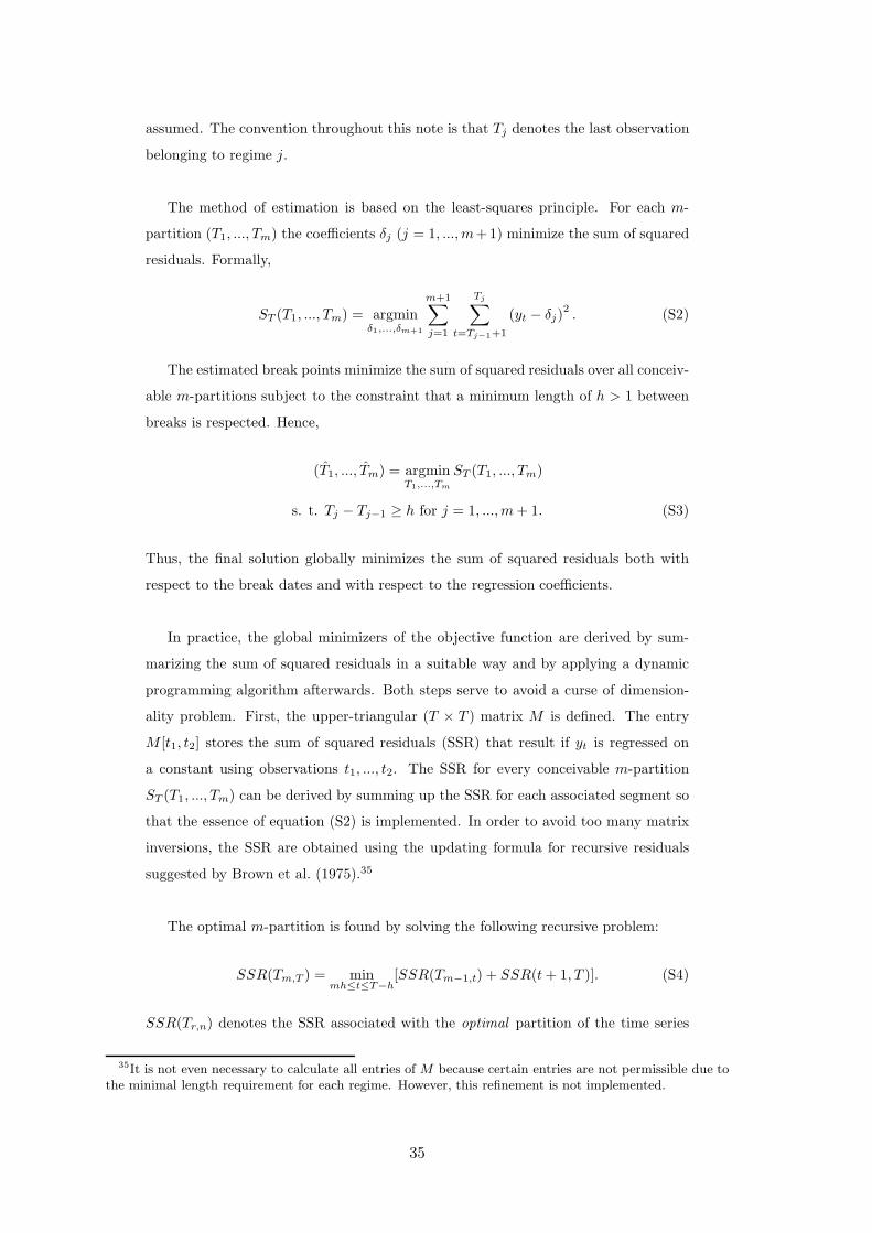
assumed. The convention throughout this note is that Tj denotes the last observation
belonging to regime j.
The method of estimation is based on the least-squares principle. For each m-
partition (T1, ..., Tm) the coefficients δj (j = 1, ...,m+1) minimize the sum of squared
residuals. Formally,
ST (T1, ..., Tm) = argminδ1,...,δm+1
m+1∑
j=1
Tj∑
t=Tj−1+1
(yt − δj)2 . (S2)
The estimated break points minimize the sum of squared residuals over all conceiv-
able m-partitions subject to the constraint that a minimum length of h > 1 between
breaks is respected. Hence,
(T1, ..., Tm) = argminT1,...,Tm
ST (T1, ..., Tm)
s. t. Tj − Tj−1 ≥ h for j = 1, ...,m+ 1. (S3)
Thus, the final solution globally minimizes the sum of squared residuals both with
respect to the break dates and with respect to the regression coefficients.
In practice, the global minimizers of the objective function are derived by sum-
marizing the sum of squared residuals in a suitable way and by applying a dynamic
programming algorithm afterwards. Both steps serve to avoid a curse of dimension-
ality problem. First, the upper-triangular (T × T ) matrix M is defined. The entry
M [t1, t2] stores the sum of squared residuals (SSR) that result if yt is regressed on
a constant using observations t1, ..., t2. The SSR for every conceivable m-partition
ST (T1, ..., Tm) can be derived by summing up the SSR for each associated segment so
that the essence of equation (S2) is implemented. In order to avoid too many matrix
inversions, the SSR are obtained using the updating formula for recursive residuals
suggested by Brown et al. (1975).35
The optimal m-partition is found by solving the following recursive problem:
SSR(Tm,T ) = minmh≤t≤T−h
[SSR(Tm−1,t) + SSR(t+ 1, T )]. (S4)
SSR(Tr,n) denotes the SSR associated with the optimal partition of the time series
35It is not even necessary to calculate all entries of M because certain entries are not permissible due tothe minimal length requirement for each regime. However, this refinement is not implemented.
35
containing r breaks and using the first n observations, SSR(t+1, T ) denotes the SSR
for the data segment starting in (t+1) and lasting until T . It is easiest to understand
the logic of the procedure by following its empirical implementation. Two further
(m + 1)× T matrices L and B are defined. Matrix L records the minimal estimated
SSR for a partition running from period 1 to the column number for a given number
of breaks, which equals the row number minus one. Matrix B stores the associated
break dates following the same conventions. It follows that the first line of matrix L
contains the estimated SSR for a sample running from period 1 to T , 1 to (T − 1) etc.
with no break and is therefore equal to the first line of matrix M . The first line in
matrix B is empty because no breaks are involved.
The second line of matrix L contains the minimal estimated SSR for a sample run-
ning from 1 to T with one structural break, the minimal estimated SSR for a sample
running from 1 to (T − 1) with one structural break and so on. The structural break
is chosen such that the estimated SSR is minimized and that the minimum duration
requirement h for each regime is respected. Hence, for the entry L[2, T ] the resulting
SSR is compared for all conceivable break dates ranging from h to (T − h) and the
break date leading to the smallest SSR is selected. This break date T1 is recorded in
B[2, T ] while the associated SSR is recorded in L[2, T ]. The other entries are derived
accordingly. For instance, for L[2, (T − 1)] and B[2, (T − 1)] the resulting SSR is
evaluated for possible break dates ranging from h to (T − h− 1).
The derivation of the third lines in L and B illustrates the working of the re-
cursive procedure. Suppose the aim is to derive L[3, T ] and B[3, T ]. Since T1 < T2
and since the minimum duration requirement for each regime has to be respected,
the second break can happen between period 2h and (T − h). The resulting SSR for
each conceivable second break date T2 in the sample running from 1 to T is given by
L[2, T2] +M [T2+1, T ]. It automatically incorporates the optimal one-break partition
for the sample spanning the observations from 1 to T2. After the SSR has been de-
rived for every conceivable second break date, the partition yielding the smallest SSR
is chosen and the associated second break date T2 and the SSR are recorded in B[3, T ]
and L[3, T ], respectively. All other entries in the second line are derived accordingly.
The same routine is repeated until m breakpoints are imposed upon the time series.
Once matrices L and B are derived, it is easy to read off the optimal break points. If
m break points are estimated, Tm is recorded in B[m + 1, T ]. The next break point
Tm−1 is found in B[m, Tm], Tm−2 is available in B[m− 1, Tm−1]. Going back step by
step the first break is obtained from B[2, T2].
36
A.2.2 Test Statistics
The test statistics in the presence of multiple structural are derived under the shrink-
ing shift asymptotic framework so that the consistency results do not directly refer to
the break dates, but to the break fractions λj = (Tj/T ) for j = 1, ...,m.36 Therefore,
the test statistics are not expressed in terms of the m-partition (T1, ..., Tm), but in
terms of the m-partition (λ1, ..., λm). Furthermore, the asymptotic distributions de-
pend on the trimming parameter ε = h/T , which is the asymptotic equivalent of the
minimum duration requirement and is necessary for the break fractions to be asymp-
totically distinct and bounded from the boundaries of the sample.
The first test statistic is called the supFT test statistic and forms the basis for
all following tests. The supF test tests the null hypothesis of no structural break
(m = 0) against the alternative hypothesis that m = k structural breaks are present.
This test is particularly useful if one has a fairly good idea a priori as to how many
breaks to expect. The supFT (k) test statistic is the supremum of all the standard F-
statistics testing the equality of means across regimes over all admissible k-partitions.
Asymptotically, the supFT (k) test statistic is equivalent to the standard F-statistic
that results if the consistently estimated break fractions (λ1, ..., λk) are used for its
construction. Hence, only the following formula needs to be evaluated in practice:
supFT (k) = FT (λ1, ..., λk) =1
T
(T − (k + 1)
k
)δ′R′(RV (δ)R′)−1Rδ. (S4)
Thereby R is the conventional restrictions matrix such that (Rδ)′ = (δ1 − δ2, ..., δk −
δk+1) and such that the estimated break fractions are respected. V (δ) is the co-
variance matrix of δ that - if desired - can be made robust to serial correlation and
heteroscedasticity. V (δ) is estimated by the standard OLS covariance matrix using all
observations if the errors are assumed to be identically distributed across segments. It
is estimated as the standard OLS covariance matrix using the data for each segment
separately if the errors are assumed to have different variances across regimes but are
serially uncorrelated. If both serial correlation and different variances across regimes
prevail, the covariance matrix is estimated using the quadratic spectral kernel based
method introduced by Andrews (1991). In this case prewhitening as in Andrews and
Monahan (1992) is recommended. The value of the supFT (k) test statistics is com-
pared to simulated critical values, which depend both on k and ε. A large test statistic
indicates that the break points significantly improve the fit of the model. Hence, in
36However, Bai and Perron (1998) show that with high probability the deviation between the estimatedand true break dates is bounded by some constant. Therefore, in empirical applications the estimatedbreak dates may be used with some confidence.
37
these cases the null hypothesis tends to be rejected.
In many interesting applications the number of breaks is not known beforehand.
In this case the double maximum tests allows to test the null hypothesis of no break
(m = 0) against the alternative of an unknown number of breaks up to K. The
test-statistic is defined as largest supFT (k) statistics for k = 1, ...,K or formally as
UDmaxFT (K) = max1≤k≤K
FT (λ1, ..., λk). (S5)
The critical values depend on K and ε. As before, a large test statistic indicates
that the null hypothesis should be rejected. The power of the double maximum test
exceeds that of the supF test if k used in the latter does not correspond with the true
number of breaks.
Ultimately, if the number of breaks is not known beforehand, the aim is to find
the appropriate number of breaks by testing. One easy way to derive the appropriate
number of breaks is to calculate the Bayesian information criterion (BIC) and choose
the number of break points which minimize the associated BIC. Formally, for a series
with k break points the BIC is defined as
BIC(k) = ln
(u′u
T
)+
(2k + 1) ln(T )
T, (S6)
with u denoting the estimated residuals accounting for the k breaks. It should be
noted that this version of the BIC penalizes each estimated coefficient and each esti-
mated break point, hence the factor (2k + 1) in the second term. The BIC performs
reasonably well in the absence of serial correlation, but tends to opt for too many
breaks in the presence of it.
A more refined method for determining the appropriate number of structural
breaks is the supFT (ℓ + 1|ℓ) sequential testing procedure, which is called supFL in
the following. Here the null hypothesis of k = ℓ breaks is tested against the alter-
native that k = ℓ + 1 breaks are present. Starting with ℓ = 0 and increasing the
number of break points one by one until the null is accepted, the number of required
breaks is derived systematically. The test is implemented as follows. If the number of
breaks under the null equals ℓ, an additional break point is introduced into each of the
ℓ+1 data segments and the corresponding supFT (1) test statistics are derived.37 The
37If the minimum duration requirement precludes the introduction of an additional break point, supFT(1)
equals zero by definition.
38
largest supFT (1) test statistic across all segments is selected and compared against
the critical values that depend on k and ε.38 The null is rejected in favor of a model
with (ℓ + 1) breaks if the overall minimal value of the SSR is sufficiently smaller the
the SSR from the model with ℓ breaks.
In some instances it may be difficult to reject the null of zero against one break,
but easy to reject the null of zero against a higher number of breaks. In these cases the
supFL testing procedure breaks down. Since the power of the double maximum test
is almost as high as the power of a test of no breaks against the alternative specifying
the true number of breaks, Bai and Perron (2006) recommend to adjust the supFL
procedure and use the double maximum test in the first step when the null hypothesis
of m = 0 breaks is tested. After this altered first step the test proceeds exactly like
the supFL test. This test is called the udmaxL test. All tests presented in this section
are implemented in the stata command sbbpm. In order to achieve as much power as
possible, the covariance matrix should be corrected for heteroscedasticity and serial
correlation whenever necessary.
A.3 Stata Implementation
A.3.1 Syntax
sbbpm depvar timevar, [minspan(#) maxbreaks(#) alpha(#) trimming(#) het(string)
prewhit(#) method(string)]
A.3.2 Description
The stata command sbbpm fits a pure multiple structural change model for means
using the methods suggested by Bai and Perron. As a minimum it requires the name
of the dependent and the time variable. The dependent variable must not contain any
missing values. The data may be tsset beforehand.
A.3.3 Options
minspan(#) specifies the minimal length h that needs to be respected between breaks.
The default value is 5.
maxbreaks(#) specifies the maximum number of breaks M that the time series may
contain. The default value is 5.
38Notice that this is equivalent to calculating the supFT(ℓ+1) test statistic using the whole time series.
39

alpha(#) specifies the significance level for the tests. The values 0.1, 0.05, 0.025 and
0.01 are allowed. The default value is 0.1.
trimming(#) specifies the trimming parameter ε that is needed for the critical val-
ues. The values 0.05, 0.10, 0.15, 0.20 and 0.25 are allowed. The default value is 0.1.
However, it is strongly recommended to adjust this default value to match ε = h/T
because otherwise wrong critical values are applied in the tests.
het(string) specifies the assumptions made with respect to the distribution of the data
and the errors across segments. If there is no serial correlation, different distributions
for the data, but identical distributions for the errors across segments, iid should be
selected. With no serial correlation in the errors, but different data and error distribu-
tions across segments, the heteroscedasticity consistent covariance matrix hc should
be selected. If in addition autocorrelation is assumed, the relevant option is the het-
eroscedasticity and autocorrelation consistent matrix hac. The default value is iid.
prewhit(#) specifies whether the heteroscedasticity and autocorrelation consistent
matrix should be derived using prewhitening. If prewhitening should be used, the
value 1 has to be entered. 0 denotes no prewhitening. The default value is 1.
method(string) specifies the methods to be applied. Possible entries are: bonly, sup,
udmax, bic, supseq, udseq. In this order they indicate to calculate the breaks only, to
apply the supFL or the UDmaxFT test, to report the BIC, to apply the original se-
quential supFT (ℓ+1|ℓ) testing procedure or the udmaxL sequential testing procedure.
The default value is bonly.
A.3.4 Saved Results
sbbpm saves in e(). The following is a complete list of saved results. The returned
results vary depending on the chosen method.
Scalars
e(baserss) SSR for model with no breaks
e(bicbreak) Final number of breaks chosen according to BIC
e(ellfinal) Final number of breaks chosen with sequential methods
Matrices
e(delta) Reports the regime-specific means for all breaks up to maxbreak breaks
40

e(var) Reports the regime-specific variance for all breaks up to maxbreak breaks
e(intervalrss) Matrix M
e(bestrss) Matrix L
e(lastbreak) Matrix B
e(breaks) Reports the break periods counted from 1 onwards for up to maxbreak breaks
according to the number of the observations
e(dates) Reports the break dates for up to maxbreak breaks
according to the time variable
e(supF res) Reports the supFL test statistics
e(udmax) Reports the largest supF-statistic for each number of
breaks up to maxbreak breaks
e(udres) Reports the results of the double maximum test
e(bic) Reports the BIC for all breaks up to maxbreak breaks
e(supFL) Reports the results of the sequential supFL test
41
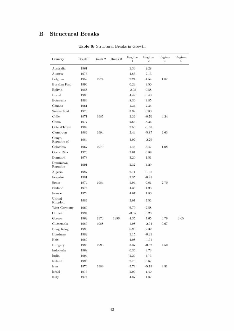
B Structural Breaks
Table 6: Structural Breaks in Growth
Country Break 1 Break 2 Break 3Regime
1Regime
2Regime
3Regime
4
Australia 1961 1.39 2.28
Austria 1973 4.83 2.13
Belgium 1959 1974 2.24 4.54 1.87
Burkina Faso 1996 0.24 3.50
Bolivia 1958 -2.08 0.58
Brazil 1980 4.49 0.40
Botswana 1989 8.30 3.85
Canada 1961 1.34 2.34
Switzerland 1973 3.32 0.80
Chile 1971 1985 2.29 -0.70 4.24
China 1977 2.63 8.36
Cote d‘Ivoire 1989 2.56 -1.66
Cameroon 1986 1994 2.44 -5.87 2.63
Congo,Republic of
1984 4.92 -2.79
Colombia 1967 1979 1.45 3.47 1.08
Costa Rica 1978 3.01 0.89
Denmark 1973 3.20 1.51
DominicanRepublic
1991 2.37 4.29
Algeria 1987 2.11 0.10
Ecuador 1981 3.35 -0.41
Spain 1974 1984 5.94 0.61 2.70
Finland 1974 4.35 1.93
France 1973 4.07 1.80
UnitedKingdom
1982 2.01 2.52
West Germany 1960 6.70 2.58
Guinea 1994 -0.55 3.28
Greece 1962 1973 1996 4.35 7.65 0.79 3.65
Guatemala 1980 1988 1.98 -2.04 0.67
Hong Kong 1988 6.93 2.32
Honduras 1982 1.15 -0.21
Haiti 1980 4.08 -1.01
Hungary 1988 1996 3.37 -0.82 4.50
Indonesia 1968 0.36 3.73
India 1994 2.29 4.73
Ireland 1993 2.76 6.67
Iran 1976 1989 5.73 -5.19 3.51
Israel 1973 5.09 1.40
Italy 1974 4.87 1.87
42
Table 6 continued
Country Break 1 Break 2 Break 3Regime
1Regime
2Regime
3Regime
4
Jamaica 1972 1980 4.28 -3.29 0.95
Jordan 1965 5.20 -0.65
Japan 1958 1970 1991 6.14 9.44 3.30 0.79
Korea,Republic of
1962 0.91 6.11
Lesotho 1978 4.37 2.31
Morocco 1958 -0.28 2.74
Madagascar 1971 0.95 -1.79
Mexico 1981 3.44 0.36
Mozambique 1995 0.38 6.39
Mauritius 1960 -4.29 3.75
Malawi 1995 1.81 -0.26
Malaysia 1970 2.77 4.88
Nigeria 1960 4.56 0.46
Nicaragua 1976 2.74 -2.38
Netherlands 1974 3.23 1.57
Norway 1986 3.28 2.29
New Zealand 1966 2.48 1.21
Pakistan 1962 1988 -0.13 3.79 1.42
Panama 1981 3.61 1.44
Peru 1975 3.21 -0.46
Philippines 1977 3.16 0.94
Poland 1978 1991 7.16 -1.05 4.06
Portugal 1973 5.90 2.25
Paraguay 1973 1981 1.06 6.12 -0.33
Romania 1979 8.09 0.95
Rwanda 1994 -1.34 11.89
Singapore 1996 5.34 1.37
Sierra Leone 1987 0.25 -3.81
El Salvador 1978 1989 1.99 -1.84 1.90
Sweden 1970 3.15 1.64
Togo 1969 5.54 -1.44
Thailand 1958 -2.36 4.75
Trinidad&Tobago
1981 1989 4.72 -5.27 5.87
Taiwan 1962 1996 4.36 7.00 3.42
Uganda 1988 -0.56 3.79
United States 1961 1.58 2.41
Venezuela 1977 2.82 -0.96
South Africa 1983 1995 1.99 -0.49 2.48
Zambia 1976 3.54 -1.33
43
C Gabon
BelgiumCanada
Switzerland
Spain
France
Gabon
United Kingdom
NetherlandsUnited States
020
000
4000
060
000
Out
put p
er W
orke
r
0 50000 100000 150000Capital Stock per Worker
Outlier Gabon
Figure 3: Observations and Frontier-Defining Countries in 1976
44
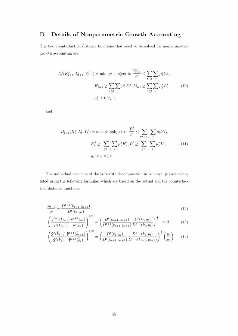
D Details of Nonparametric Growth Accounting
The two counterfactual distance functions that need to be solved for nonparametric
growth accounting are
Djt (K
jt+1, L
jt+1;Y
jt+1) = min φj subject to
Y jt+1
φj≤∑
τ≤t
∑
j
µjτY
jτ ,
Kjt+1 ≥
∑
τ≤t
∑
j
µjτK
jτ , L
jt+1 ≥
∑
τ≤t
∑
j
µτjL
jτ , (10)
µjτ ≥ 0 ∀j, τ,
and
Djt+1(K
jt , L
jt ;Y
jt ) = min φj subject to
Y jt
φj≤∑
τ≤t+1
∑
j
µjτY
jτ ,
Kjt ≥
∑
τ≤t+1
∑
j
µjτK
jτ , L
jt ≥
∑
τ≤t+1
∑
j
µτjL
jτ , (11)
µjτ ≥ 0 ∀j, τ.
The individual elements of the tripartite decomposition in equation (6) are calcu-
lated using the following formulas, which are based on the actual and the counterfac-
tual distance functions:
φt+1
φt=
Dt+1(kt+1, yt+1)
Dt(kt, yt), (12)
(yt+1(kt+1)
yt(kt+1)
yt+1(kt)
yt(kt)
)1/2
=
(Dt(kt+1, yt+1)
Dt+1(kt+1, yt+1)
Dt(kt, yt)
Dt+1(kt, yt)
) 12
, and (13)
(yt(kt+1)
yt(kt)
yt+1(kt+1)
yt+1(kt)
)1/2
=
(Dt(kt, yt)
Dt(kt+1, yt+1)
Dt+1(kt, yt)
Dt+1(kt+1, yt+1)
) 12(ycyb
)(14)
45
Recommended