INSTITUTE OF PHYSICS PUBLISHING JOURNAL OF PHYSICS D: APPLIED PHYSICS
J. Phys. D: Appl. Phys. 35 (2002) 1149–1163 PII: S0022-3727(02)31310-X
Analysis of phase-resolved partialdischarge patterns of voids based on astochastic process approach
R Altenburger1, C Heitz2 and J Timmer1
1 Freiburg Center of Data Analysis and Modeling, Germany2 Institute of Data Analysis and Process Design, Zurich University of Applied Sciences
Winterthur, Switzerland
Received 28 November 2001, in final form 3 April 2002Published 21 May 2002Online at stacks.iop.org/JPhysD/35/1149
AbstractA method is presented for the determination of physical dischargeparameters for partial discharges (PDs) of voids in solid insulation. Basedon a recently developed stochastic theory of PD processes, a statisticalanalysis of a measured phase-resolved partial discharge (PRPD) patternallows the determination of the relevant physical parameters like firstelectron availability or decay time constants for deployed charge carriers.These parameters can be estimated directly from the measured patternswithout the need of performing simulations. Furthermore, error bounds forthe parameter values can be given.
The parameter estimation algorithm is based on the analysis of acontiguous region of the PRPD pattern where this region can be chosennearly arbitrarily. Thus, even patterns with several active PD defects orpatterns which are corrupted by noise can be analysed.
The method is applied to a sequence of patterns of a void in epoxy resin.The change in first electron availability in the course of a day can bedetermined quantitatively from the data while the other physical parametersremain constant.
1. Introduction
Much work has been established in the last two decades in
order to understand and describe the nature of partial discharge
(PD) processes [1–9]. For some discharge phenomena physical
models have been developed (e.g. [2, 5, 22, 27]). These
models have substantially increased the knowledge of the
physical processes during PD processes. For the analysis
and interpretation of measured PD data, this knowledge is
fundamental. It allows to extract information about the
physical situation at the PD defect.
On the other hand, different PD measuring systems have
been developed which allow the detection and recording of
PDs. These systems are now widely used for monitoring and
failure detection in high-voltage equipment. Especially phase-
resolved partial discharge (PRPD) measurement systems have
become very popular.
However, the analysis and interpretation of measured PD
data is still a difficult task. Many publications treat this
problem (e.g. [10–29]). Two different kinds of analysis meth-
ods are used: the first method is based on a description of
the PD data by means of a set of parameters which, in most
cases, are statistical features [13–21], e.g. the number of dis-
charges per period, skewness and kurtosis of the pulse height
or phase-distribution, and others. These parameters yield a
characterization of the PD pattern and can thus be used for
interpretation and classification tasks. The main disadvantage
of such a purely descriptive characterization is the fact that the
parameters are not physical parameters, making an interpreta-
tion difficult. For example, an increase of the applied voltage
may lead to other values of the statistical parameters, even if
the physics of the discharge does not change significantly.
In contrast, the second analysis method is based on a
physical model which is used to perform simulations of the PD
process. Comparison of the simulated data with the measured
ones allows for the determination of the physical parameters.
Examples of this approach are [22–29]. This approach
renders a characterization of the pattern by physical parameters
0022-3727/02/111149+15$30.00 © 2002 IOP Publishing Ltd Printed in the UK 1149
R Altenburger et al
which, in most cases, is more useful than a purely descriptive
characterization. However, the simulation–comparison
method is difficult to use since there is no systematic way to
find the correct parameter settings. Most often, the parameters
are found by trial and error. This prevents the physical method
to be used in automatic pattern analysis algorithms.
In this paper, a new method is presented which allows the
extraction of physical discharge parameters from measured PD
data in a systematic and automatic way, based on the analysis
of PRPD patterns. It is based on a newly developed description
of the PD process [8] which is consequently formulated in a
stochastic framework. The discharge process is assumed to be
governed by few pysical parameters the most important ones
are the first electron availability and the charge removal after
a discharge.
By statistical data analysis of the measured pattern, the
values of the physical parameters can be extracted directly
from a measured PRPD pattern. Thus, a characterization
by physical parameters can be obtained without the need of
simulation. This overcomes one of the major restrictions
of the above-mentioned physically based analysis methods.
It thus combines the advantage of the purely descriptive
method (possibility of automated parameter extraction)
with the advantage of the physical model-based approach
(characterization by physically meaningful parameters).
The method is explicitely worked out for the case of void
discharges with constant first electron supply rate. However,
as will be shown in section 3.6, it can be extended to non-
constant hazard rate. Furthermore, the idea of the parameter
estimation method could be used for other kinds of discharges
like surface discharges or corona discharges.
The new method of data analysis has the advantageous
property that it can be applied even to small parts of the pattern.
Thus, it is possible to analyse separately different PD sources
which are separated in the PRPD pattern. Furthermore, it is
possible to deal with disturbances which, in practice, cannot
be avoided. Therefore, the method is not restricted to the
laboratory but can be used in the daily engineering work.
The paper is structured as follows: in section 2 the
description of the PD process as a stochastic process will be
reviewed briefly. In sections 3 and 4 the new method of data
analysis is described. In section 5 the method is applied to
simulated data, while in section 6 the application to measured
PD patterns is shown.
2. PD process as a stochastic process
The presented pattern analysis method is based on a recently
developed description of the PD process as a stochastic process
which will be reviewed briefly in the following. For details,
the reader is referred to the original paper [8]. Within this
paper, the discussion is restricted to the case of void discharges.
However, the original model is more general and can be applied
to other kinds of discharges as well.
The PD process consists of the sequence of electrical
discharges under an externally applied electrical field E0(t).
The discharges (PD events) lead to a charge deployment in the
vicinity of the PD defect which give rise to a so-called internal
field Ei(t). Each PD event changes the internal field suddenly.
Between the successive PD events, the internal field changes
due to charge dissipation mechanisms like surface conduction
in voids, or charge carrier drift in gas discharges. The PD
process itself can thus be described by the evolution of the
internal field Ei(t). The dynamics of this process is described
briefly in the following.
During a discharge at time t the total electric field Etot(t),
Etot(t) = E0(t) + Ei(t), (1)
drops to a residual field Eres:
Etot �→ E′tot = ±Eres. (2)
The positive sign is chosen if Etot(t) > 0 and vice versa. The
value Eres of the residual field is defect specific. It is assumed
that the residual field has a constant value for each discharge.
With equation (2) a discharge leads to a sudden jump in Ei:
Ei(t) �→ E′i(t) = ±Eres − E0(t). (3)
The bipolar charge distribution deployed in the vicinity of the
PD defect tends to vanish by drift and recombination processes.
In general, it can be described by a differential equation:
Ei(t) = f (Ei(t), E0(t)). (4)
In contrast to the jump process during a PD event, this field
change is continuous and deterministic until the next PD event
takes place. A simplification consists in setting
f = −Ei/τ, (5)
leading to an exponential decay with a single time constant τ
which does not depend on Ei and E0:
Ei(t) = Ei(t0)e−t/τ .
In this simplification, the drift and recombination process is
subsumed by a single parameter τ which is a time constant
for the charge decay process. Note that this only can be
a very rough approximation to the real physical drift and
recombination processes which cannot take into acount the
detailed physical processes. Examples are field-dependent
surface conduction, or shielding effects due to conductivity of
cavity walls. On the other hand, the parameter τ has a direct
physical meaning. For different kinds of discharges, the time
constant for the decay of internal charge can be very different.
For example, for a void discharge, where the internal charge
may decay by surface conduction, the time constant is of the
order of magnitude of minutes or hours.
Both processes, discharge ( jump of Ei) and drift/
recombination (continuous change of Ei), interact in a real PD
process. They are coupled by the discharge probability in the
following way: let c dt be the probability that a fast discharge
occurs in the time interval [t, t + dt]. This probability may
depend on the internal field Ei(t) as well as on the external field
E0(t) and depends on the mechanism of first electron supply
[8]. For a void where starting electrons are supplied mainly by
external radiation, we have c = 0 for Etot < Einc with a typical
inception field Einc, and c = const for Etot > Einc. The value
of c depends on the void volume and the electron production
rate of the externally imposed radiation [5].
1150
Analysis of PRPD patterns of voids
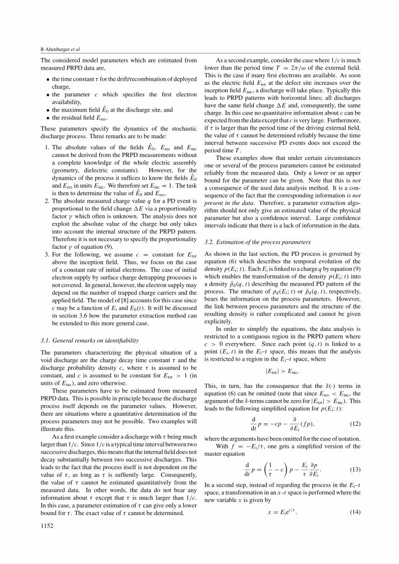
For a small time step dt the time evolution of Ei(t) is
shown schematically in figure 1. Two different paths are
possible: a fast discharge, or a slow discharge due to drift
and recombination. The probability for each path is c dt and
1 − c dt , respectively. In figure 2 typical (random) trajectories
of Etot(t) and Ei(t) for the case of AC voltage are shown.
Note that the same process realization is shown in figures 2(a)
and (b).
The dynamics of the internal field forms a piecewise
deterministic Markov process [30]. Such processes are
generally described by a dynamical equation for the time-
dependent probability density p(Ei; t). From the short-time
dynamics of the stochastic process as sketched in figure 1,
a differential equation for p(Ei; t) can be constructed, the
so-called master equation [31]. For the considered PD system
one gets (see [8] for details)
∂
∂tp(Ei; t) = −c(Ei, E0(t)) · p(Ei; t)
−∂
∂Ei
(f (Ei, E0(t)) · p(Ei; t))
+(
∫
E′i +E0(t)>0
c(E′i, E0(t)) · p(E′
i; t) dE′i
)
·δ(Ei − (Eres − E0(t)))
+(
∫
E′i +E0(t)<0
c(E′i, E0(t)) · p(E′
i; t) dE′i
)
·δ(Ei − (−Eres − E0(t))), (6)
where δ(·) is the Kronecker delta function.
Figure 1. Time evolution of Ei(t) to Ei(t + dt) for small dt . Theupper path with probability c dt represents the change of Ei(t) dueto a discharge, the lower path with probability 1 − c dt is the timedevelopment for the case of no discharge.
(a)
(b)
Figure 2. Typical trajectories under AC for (a) Etot(t) =E0(t) + Ei(t) and (b) Ei(t).
From p(Ei; t) one can derive the probability density
pd(Ei, t) of a PD event at time t and internal field Ei (the
subscript d stands for discharge)
pd(Ei; t) = c(Ei, E0(t)) · p(Ei; t). (7)
Until now, the dynamics of the PD system has been formulated
in terms of the internal field Ei(t). However, with the usual
PD measuring technique Ei(t) cannot be measured, i.e. the
PD process cannot be observed directly. Instead, the charge
separation of the bipolar charge quantity ±q being deployed
during the discharge is measured.
The jump �E of the internal field during a fast discharge
according to equation (3) is given by
�E = E′i − Ei = ±Eres − (Ei + E0(t)). (8)
This field change is accomplished by the deployment of
a bipolar charge quantity which, for a void discharge, is
proportional to the field change [8]. The measured charge q,
in turn, is proportional to the deployed charge, leading to
q = −γ · �E = γ (Ei + E0(t)µEres). (9)
The proportionality factor γ not only depends on the void
geometry but also on the electromagnetic coupling of the void
to the PD detector [37, 38]. Given the field Ei just before the
discharge and the external field E0 at the discharge time, the
charge q can be calculated. The minus sign in the first line of
equation (9) accounts for the usual convention that a charge
is considered positive if the field change is negative, and vice
versa.
The probability density pd(Ei; t) can be transformed into
the probability density pd(q, t) of a discharge with specified
charge q at time t :
pd(q, t) = pd(Ei(q), t)dEi
dq. (10)
For AC voltages, the so-called PRPD patterns correspond to
pd(q, t) for t ∈ [0, T ] or p(q, ϕ) for ϕ ∈ [0, 2π ], respectively.
When measuring a PRPD pattern, one plots each measured
PD event (t, q) in the ϕ–q plane, where ϕ is the phase angle
of the discharge time t . Thus, the point density of a PRPD
pattern directly corresponds to the probability density pd(q, t)
of the generating PD process. This yields the possibility of
extracting the physical parameters of the model from measured
PRPD data.
3. Determination of parameters from measuredPRPD data
In this section the new method for extracting the physical
parameters of the discharge directly from the measured PRPD
pattern is presented. This method is described for the case of
void discharges with a constant rate of initial electrons. It can
be extended to the case of non-constant hazard rate as will be
discussed in section 3.6.
We consider the case of sinusoidal external voltage,
leading to a field
E0(t) = E0 sin(ωt). (11)
1151
R Altenburger et al
The considered model parameters which are estimated from
measured PRPD data are,
• the time constant τ for the drift/recombination of deployed
charge,
• the parameter c which specifies the first electron
availability,
• the maximum field E0 at the discharge site, and
• the residual field Eres.
These parameters specify the dynamics of the stochastic
discharge process. Three remarks are to be made:
1. The absolute values of the fields E0, Eres and Einc
cannot be derived from the PRPD measurements without
a complete knowledge of the whole electric assembly
(geometry, dielectric constants). However, for the
dynamics of the process it suffices to know the fields E0
and Eres in units Einc. We therefore set Einc = 1. The task
is then to determine the value of E0 and Eres.
2. The absolute measured charge value q for a PD event is
proportional to the field change �E via a proportionality
factor γ which often is unknown. The analysis does not
exploit the absolute value of the charge but only takes
into account the internal structure of the PRPD pattern.
Therefore it is not necessary to specify the proportionality
factor γ of equation (9).
3. For the following, we assume c = constant for Etot
above the inception field. Thus, we focus on the case
of a constant rate of initial electrons. The case of initial
electron supply by surface charge detrapping processes is
not covered. In general, however, the electron supply may
depend on the number of trapped charge carriers and the
applied field. The model of [8] accounts for this case since
c may be a function of Ei and E0(t). It will be discussed
in section 3.6 how the parameter extraction method can
be extended to this more general case.
3.1. General remarks on identifiability
The parameters characterizing the physical situation of a
void discharge are the charge decay time constant τ and the
discharge probability density c, where τ is assumed to be
constant, and c is assumed to be constant for Etot > 1 (in
units of Einc), and zero otherwise.
These parameters have to be estimated from measured
PRPD data. This is possible in principle because the discharge
process itself depends on the parameter values. However,
there are situations where a quantitative determination of the
process parameters may not be possible. Two examples will
illustrate this.
As a first example consider a discharge with τ being much
larger than 1/c. Since 1/c is a typical time interval between two
successive discharges, this means that the internal field does not
decay substantially between two successive discharges. This
leads to the fact that the process itself is not dependent on the
value of τ , as long as τ is suffiently large. Consequently,
the value of τ cannot be estimated quantitatively from the
measured data. In other words, the data do not bear any
information about τ except that τ is much larger than 1/c.
In this case, a parameter estimation of τ can give only a lower
bound for τ . The exact value of τ cannot be determined.
As a second example, consider the case where 1/c is much
lower than the period time T = 2π/ω of the external field.
This is the case if many first electrons are available. As soon
as the electric field Etot at the defect site increases over the
inception field Einc, a discharge will take place. Typically this
leads to PRPD patterns with horizontal lines; all discharges
have the same field change �E and, consequently, the same
charge. In this case no quantitative information about c can be
expected from the data except that c is very large. Furthermore,
if τ is larger than the period time of the driving external field,
the value of τ cannot be determined reliably because the time
interval between successive PD events does not exceed the
period time T .
These examples show that under certain circumstances
one or several of the process parameters cannot be estimated
reliably from the measured data. Only a lower or an upper
bound for the parameter can be given. Note that this is not
a consequence of the used data analysis method. It is a con-
sequence of the fact that the corresponding information is not
present in the data. Therefore, a parameter extraction algo-
rithm should not only give an estimated value of the physical
parameter but also a confidence interval. Large confidence
intervals indicate that there is a lack of information in the data.
3.2. Estimation of the process parameters
As shown in the last section, the PD process is governed by
equation (6) which describes the temporal evolution of the
density p(Ei; t). Each Ei is linked to a charge q by equation (9)
which enables the transformation of the density p(Ei; t) into
a density pd(q, t) describing the measured PD pattern of the
process. The structure of pd(Ei; t) or pd(q, t), respectively,
bears the information on the process parameters. However,
the link between process parameters and the structure of the
resulting density is rather complicated and cannot be given
explicitely.
In order to simplify the equations, the data analysis is
restricted to a contiguous region in the PRPD pattern where
c > 0 everywhere. Since each point (q, t) is linked to a
point (Ei, t) in the Ei–t space, this means that the analysis
is restricted to a region in the Ei–t space, where
|Etot| > Einc.
This, in turn, has the consequence that the δ(·) terms in
equation (6) can be omitted (note that since Eres < Einc, the
argument of the δ-terms cannot be zero for |Etot| > Einc). This
leads to the following simplified equation for p(Ei; t):
d
dtp = −cp −
∂
∂Ei
(fp), (12)
where the arguments have been omitted for the ease of notation.
With f = −Ei/τ , one gets a simplified version of the
master equation
d
dtp =
(
1
τ− c
)
p −Ei
τ
∂p
∂Ei
. (13)
In a second step, instead of regarding the process in the Ei–t
space, a transformation in an x–t space is performed where the
new variable x is given by
x = Eiet/τ . (14)
1152
Analysis of PRPD patterns of voids
Under this transformation, the dynamical equation
(equation (13)) transforms to the simple form (see appendix A)
d
dtp(x; t) = −c(x, t)p(x; t), (15)
where p(x; t) is the time-dependent probability density
function of the variable x. This equation can be solved
analytically. For the case of void discharges where c =
constant for Etot > Einc, one gets
p(x; t) = A(x)e−ct . (16)
Thus, in the x–t space, the the state density has a product form.
Similar to the discussion in section 2, this probability
density is a density of the possible states of the stochastic
process. The density of actually observed PD events is given by
pd(x, t) = c(x, t)p(x; t). (17)
Recall that c is assumed to be either zero or a constant. In
regions where c > 0, pd(x, t) differs from p(x, t) only by a
proportionality factor. Thus
pd(x, t) = A(x)e−ct (18)
within this region with a function A(x). Again a simple product
form is obtained.
For summarizing we conclude that by a variable
transformation q → x according to
Ei = ±Eres − E0 −q
γ,
x = Eiet/τ ,
(19)
the density pd(q, t) transforms into the density pd(x, t) which
has a simple product form. The time dependence consists of
an exponential decay e−ct with an initial density A(x).
The same transformation can be performed on a measured
PRPD pattern. Each PD event (q, t) is represented by an event
in x–t space with the transformations equation (19). Thus,
PRPD pattern is transformed into a point pattern in the x–t
space.
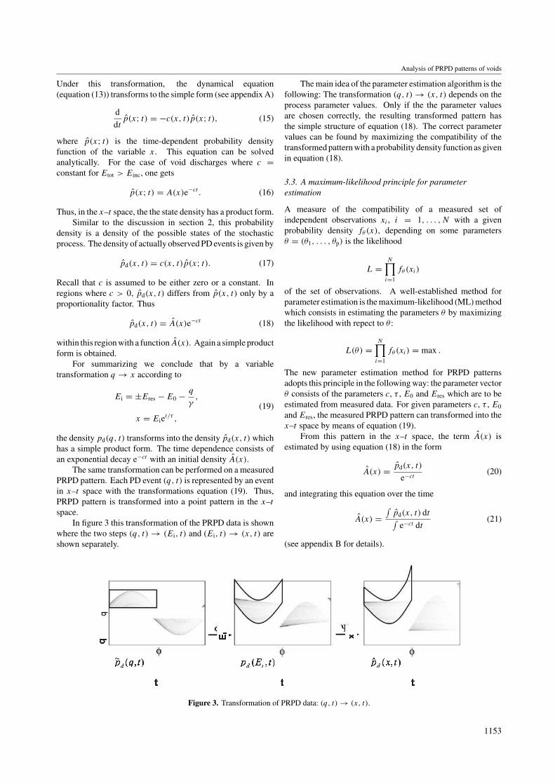
In figure 3 this transformation of the PRPD data is shown
where the two steps (q, t) → (Ei, t) and (Ei, t) → (x, t) are
shown separately.
Figure 3. Transformation of PRPD data: (q, t) → (x, t).
The main idea of the parameter estimation algorithm is the
following: The transformation (q, t) → (x, t) depends on the
process parameter values. Only if the the parameter values
are chosen correctly, the resulting transformed pattern has
the simple structure of equation (18). The correct parameter
values can be found by maximizing the compatibility of the
transformed pattern with a probability density function as given
in equation (18).
3.3. A maximum-likelihood principle for parameter
estimation
A measure of the compatibility of a measured set of
independent observations xi , i = 1, . . . , N with a given
probability density fθ (x), depending on some parameters
θ = (θ1, . . . , θp) is the likelihood
L =
N∏
i=1
fθ (xi)
of the set of observations. A well-established method for
parameter estimation is the maximum-likelihood (ML) method
which consists in estimating the parameters θ by maximizing
the likelihood with repect to θ :
L(θ) =
N∏
i=1
fθ (xi) = max .
The new parameter estimation method for PRPD patterns
adopts this principle in the following way: the parameter vector
θ consists of the parameters c, τ , E0 and Eres which are to be
estimated from measured data. For given parameters c, τ , E0
and Eres, the measured PRPD pattern can transformed into the
x–t space by means of equation (19).
From this pattern in the x–t space, the term A(x) is
estimated by using equation (18) in the form
A(x) =pd(x, t)
e−ct(20)
and integrating this equation over the time
A(x) =
∫
pd(x, t) dt∫
e−ct dt(21)
(see appendix B for details).
1153

R Altenburger et al
Figure 4. Estimation of A(x) from the transformed data.
The enumerator of equation (21) can be estimated from the
measured data via a kernel estimator [32]. The denominator
is known for specified model parameters. As an example,
figure 4 shows the transformed data and an estimate of the
initial distribution A(x).
The likelihood of the measured set of PD events is
now calculated by treating each PD event as an independent
realization of an underlying two-dimensional density function
pd(x, t):
L(c, τ, E0, Eres) =
N∏
i=1
p(c,τ,E0,Eres)(xi, ti), (22)
where (xi, ti), i = 1, . . . , N , denote the single PD events in
the x–t space, and pd(x, t) is given by equation (18), using the
estimate of A(x).
Maximizing this likelihood with respect to the process
parameters leads to the estimates of the parameters.
Schematically the whole procedure is as follows:
1. transform data (qi, ti) → (xi, ti) (depending on Eres, Ea
and τ),
2. estimate A(x),
3. pd(x, t) = A(x)e−ct ,
4. L(c, τ, E0, Eres) =∏N
i=1 p(c,τ,E0,Eres)(xi, ti).
The parameters Eres, Ea and τ contribute to the likelihood
function L via the transformation (qi, ti) → (xi, ti) and the
estimation of A(x). The likelihood function is maximized by
a standard optimization algorithm [33].
3.4. Confidence intervals
To obtain confidence intervals for the estimated parameter,
a non-parametric bootstrap method is applied [34]. If the
original data set D consists of N data points, M new data
sets, D1, . . . , DM , each with N data points are drawn from
the original set with replacement. From each new data
set parameters Θ∗i are estimated. Those will be distributed
around the original estimated parameters Θ with a particular
distribution. Confidence intervals can be obtained from the
quantiles of that distribution [34].
3.5. Discussion of the parameter estimation method
In this section, some remarks on the parameter estimation
method are made.
First, a remark on the statistical methodology must be
made. The above-applied method for parameter estimation
by maximizing L(c, τ, E0, Eres) in equation (22) is, strictly
speaking, not identical to the usual ML method, since for the
density pd(x, t) the function A(x) is used which is estimated
from the measured data. However, for large samples, the
kernel estimator for A(x) yields the correct density. Thus,
asymptotically, the likelihood is calculated correctly.
A second remark must be made on the estimation of the
fields E0, Eres and Einc. As explained in section 3, these
fields cannot be determined in their absolute values (i.e. in
units V m−1). From a practical point of view, it would be
desirable to get E0 and Eres in units Einc which only requires
the determination of the ratios of the fields.
With the parameter estimation method as described above,
it is not possible to extract the value of Einc. This is due to
the fact that the parameter estimation algorithm is based on
data analysis in a region of the PRPD pattern where c > 0.
On the other hand, the inception field Einc is specified by
the field value where c drops down to zero. Since this is
outside of the analysed region, the estimation algorithm cannot
determine Einc.
However, Einc can be calculated from the minimum
measured charge qmin. For simplification, we restrict the
discussion to positive discharges. Setting Etot = Ei + E0 to its
minimum value Einc in equation (9), one gets
qmin = γ (Einc − Eres). (23)
Usually the minimum charge qmin can be determined quite
well from the measured PRPD pattern. Once Eres has been
estimated by the parameter estimation algorithm, the field
Einc can be calculated in the same units as the field Eres by
determining the minimum charge qmin from the measured PD
pattern. With this information the fields E0 and Eres can be
given in units of Einc.
Thus, an additional input for the parameter estimation
algorithm is the specification of qmin. Note that this
information is not necessary for the parameter estimation itself,
but only for calculating the correct units for the estimated fields.
3.6. Extension of the parameter estimation method to
non-constant hazard rate
The parameter estimation algorithm has been developed for
the case of a constant first electron supply, i.e. a constant value
of the parameter c. It can, however, be extended to the case of
non-constant hazard rate as will be shown in the following.
For the case of a non-constant hazard rate which depends
on the number of trapped charges and the applied external field,
the parameter c is a function of Ei and E0(t), or, equivalently,
on Ei and t : c = c(Ei; t). This means that the single parameter
c is replaced by a function which has many degress of freedom.
For the following we assume that this function c(Ei; t) is
parametrized by some parameters ψ = (ψ1, ψ2, . . .). Instead
of estimating one single value c, the task of the parameter
estimation procedure is to estimate the parameter vector ψ ,
describing the mechanism of first electron supply.
For doing this, the above described parameter estimation
method has to be modified only slightly. The transformation
from the pattern p(Ei; t) to the pattern p(x; t) can be made
1154
Analysis of PRPD patterns of voids
exactly like for the case of constant c since this transformation
does not require c to be constant.
A difference arises in equation (16) which is replaced by
p(x; t) = A(x) exp
(
−
∫ t
0
c(x, t ′) dt ′)
, (24)
where the function c(Ei; t) has been transformed into the
function c(x, t). The discharge event density pd(x, t) is then
given by
pd(x, t) = c(x, t)A(x) exp
(
−
∫ t
0
c(x, t ′) dt ′)
, (25)
and the function A(x) can be estimated using the equation
A(x) =
∫
pd(x, t) dt∫
c(x, t) exp (−∫
c(x, t)t ′ dt ′) dt. (26)
For given c(x, t), or, equivalently, for a given parameter
vector ψ , the function A(x) can be estimated as before from
the transformed pattern. The calculation of the likelihood can
then be performed identically as for the case of constant c.
The model parameters are estimated by maximizing the
loglikelihood with respect to the model parameters Eres, Ea, τ
and ψ .
Thus, the parameter estimation algorithm for non-constant
hazard rate is identical to the case of constant hazard rate
except that equations (18) and (21) have to be replaced by
equations (25) and (26), and the single parameter c is replaced
by a set of parameters ψ = (ψ1, ψ2, . . . ).
4. The holographic property of the parameterestimation algorithm
In the last sections a new algorithm for estimating parameters
of a PD process has been presented. Basically, it consists of a
ML approach which has to be applied to a contigueous region
of the PD pattern for which c > 0 is guaranteed. Such regions
can be easily found in a measured PD pattern since c must be
positive in all regions where actually PD events are recorded.
Aditionally, if positive charges are recorded at a point (q, t),
then c > 0 for all point (q ′, t) with q ′ > q.
The simplest possibility of a contiguous region with c > 0
is to take the whole positive or negative part of the pattern
with exception of the horizontal zone around q = 0 where
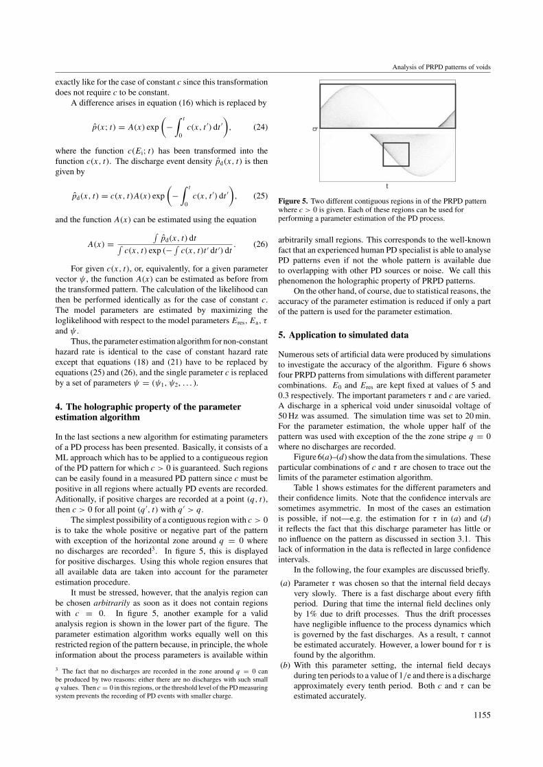
no discharges are recorded3. In figure 5, this is displayed
for positive discharges. Using this whole region ensures that
all available data are taken into account for the parameter
estimation procedure.
It must be stressed, however, that the analyis region can
be chosen arbitrarily as soon as it does not contain regions
with c = 0. In figure 5, another example for a valid
analysis region is shown in the lower part of the figure. The
parameter estimation algorithm works equally well on this
restricted region of the pattern because, in principle, the whole
information about the process parameters is available within
3 The fact that no discharges are recorded in the zone around q = 0 can
be produced by two reasons: either there are no discharges with such small
q values. Then c = 0 in this regions, or the threshold level of the PD measuring
system prevents the recording of PD events with smaller charge.
Figure 5. Two different contiguous regions in of the PRPD patternwhere c > 0 is given. Each of these regions can be used forperforming a parameter estimation of the PD process.
arbitrarily small regions. This corresponds to the well-known
fact that an experienced human PD specialist is able to analyse
PD patterns even if not the whole pattern is available due
to overlapping with other PD sources or noise. We call this
phenomenon the holographic property of PRPD patterns.
On the other hand, of course, due to statistical reasons, the
accuracy of the parameter estimation is reduced if only a part
of the pattern is used for the parameter estimation.
5. Application to simulated data
Numerous sets of artificial data were produced by simulations
to investigate the accuracy of the algorithm. Figure 6 shows
four PRPD patterns from simulations with different parameter
combinations. E0 and Eres are kept fixed at values of 5 and
0.3 respectively. The important parameters τ and c are varied.
A discharge in a spherical void under sinusoidal voltage of
50 Hz was assumed. The simulation time was set to 20 min.
For the parameter estimation, the whole upper half of the
pattern was used with exception of the the zone stripe q = 0
where no discharges are recorded.
Figure 6(a)–(d) show the data from the simulations. These
particular combinations of c and τ are chosen to trace out the
limits of the parameter estimation algorithm.
Table 1 shows estimates for the different parameters and
their confidence limits. Note that the confidence intervals are
sometimes asymmetric. In most of the cases an estimation
is possible, if not—e.g. the estimation for τ in (a) and (d)
it reflects the fact that this discharge parameter has little or
no influence on the pattern as discussed in section 3.1. This
lack of information in the data is reflected in large confidence
intervals.
In the following, the four examples are discussed briefly.
(a) Parameter τ was chosen so that the internal field decays
very slowly. There is a fast discharge about every fifth
period. During that time the internal field declines only
by 1% due to drift processes. Thus the drift processes
have negligible influence to the process dynamics which
is governed by the fast discharges. As a result, τ cannot
be estimated accurately. However, a lower bound for τ is
found by the algorithm.
(b) With this parameter setting, the internal field decays
during ten periods to a value of 1/e and there is a discharge
approximately every tenth period. Both c and τ can be
estimated accurately.
1155
R Altenburger et al
Figure 6. Simulated data for different parameter combinations of τ and c.
Table 1. True values and estimates of parameters c, τ , E0 and Eres for simulated data.
c cest τ τ (estim.) E0 E0 (estim.) Eres Eres (estim.)Figure (s−1) (s−1) (s) (s) (Einc) (Einc) (Einc) (Einc)
(a) 10 13.6 ± 4.5 10 140+∞−135 5 5.01 ± 0.02 0.3 0.29 ± 0.02
(b) 10 13.18 ± 4.7 0.2 0.22 ± 0.03 5 4.97+0.04−0.1 0.3 0.3 ± 0.01
(c) 250 249.5 ± 1.5 0.1 0.098 ± 0.003 5 5.01 ± 0.03 0.3 0.3 ± 0.01(d) 5000 4950 ± 30 0.1 0.2+∞
−0.15 5 6 ± 3 0.3 0.2 ± 0.2
(c) τ is similar to the value in (b). The internal field decays
during five periods to a value of 1/e—c is higher. The
parameters can be estimated with high precision.
(d) c is extremely high. As soon as the total field exceeds the
inception field, a discharge takes place. Drift processes
have no influence to the process dynamics. Thus τ cannot
be estimated.
In all cases, the values of E0 and Eres could be determined
with a high accuracy.
As an example of the holographic property, in figure 7 the
estimated parameter values for two different analysis regions
are shown. It can be seen that the parameter estimation
works well for both regions. However, the smaller the region,
the larger are the error bounds because fewer data enter the
analyis.
6. Application to measured data
The algorithm was applied to data obtained from an artificial
spherical void in epoxy resin under sinusoidal voltage.
Seventy-two measurement were made during 24 h (20 min
per measurement) at constant voltage level [35]. The PRPD
patterns are provided as a 256×256 numerical array where each
bin is specified by its phase position and the charge amplitude
Figure 7. Holographic property.
and contains the number of recorded PD events for this phase
position and charge. In [36], the details on the experimental
setup and the measurement method can be found. Figure 8
shows a selection of these measurements.
The PRPD patterns can be divided into two groups.
Measurements 1–22 and 49–72 (group I) show nearly identical
1156
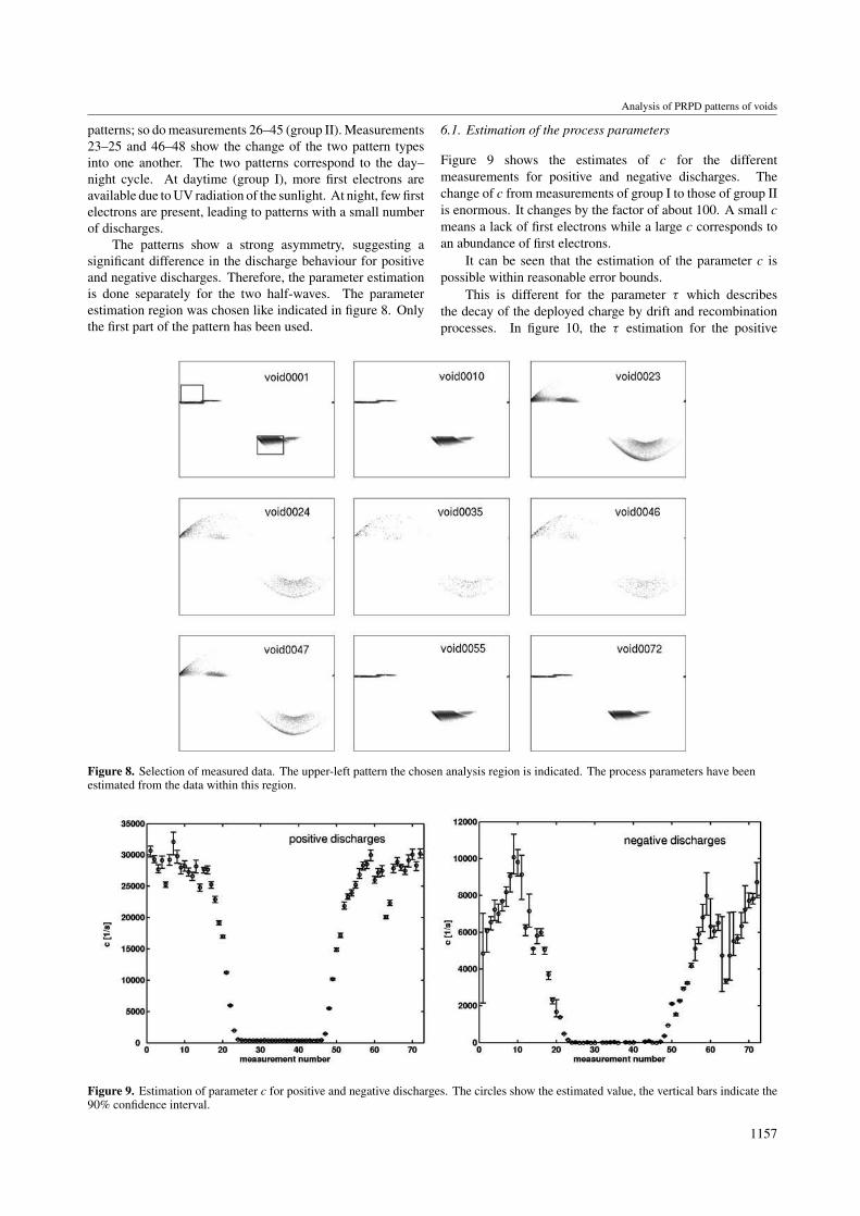
Analysis of PRPD patterns of voids
patterns; so do measurements 26–45 (group II). Measurements
23–25 and 46–48 show the change of the two pattern types
into one another. The two patterns correspond to the day–
night cycle. At daytime (group I), more first electrons are
available due to UV radiation of the sunlight. At night, few first
electrons are present, leading to patterns with a small number
of discharges.
The patterns show a strong asymmetry, suggesting a
significant difference in the discharge behaviour for positive
and negative discharges. Therefore, the parameter estimation
is done separately for the two half-waves. The parameter
estimation region was chosen like indicated in figure 8. Only
the first part of the pattern has been used.
Figure 8. Selection of measured data. The upper-left pattern the chosen analysis region is indicated. The process parameters have beenestimated from the data within this region.
Figure 9. Estimation of parameter c for positive and negative discharges. The circles show the estimated value, the vertical bars indicate the90% confidence interval.
6.1. Estimation of the process parameters
Figure 9 shows the estimates of c for the different
measurements for positive and negative discharges. The
change of c from measurements of group I to those of group II
is enormous. It changes by the factor of about 100. A small c
means a lack of first electrons while a large c corresponds to
an abundance of first electrons.
It can be seen that the estimation of the parameter c is
possible within reasonable error bounds.
This is different for the parameter τ which describes
the decay of the deployed charge by drift and recombination
processes. In figure 10, the τ estimation for the positive
1157
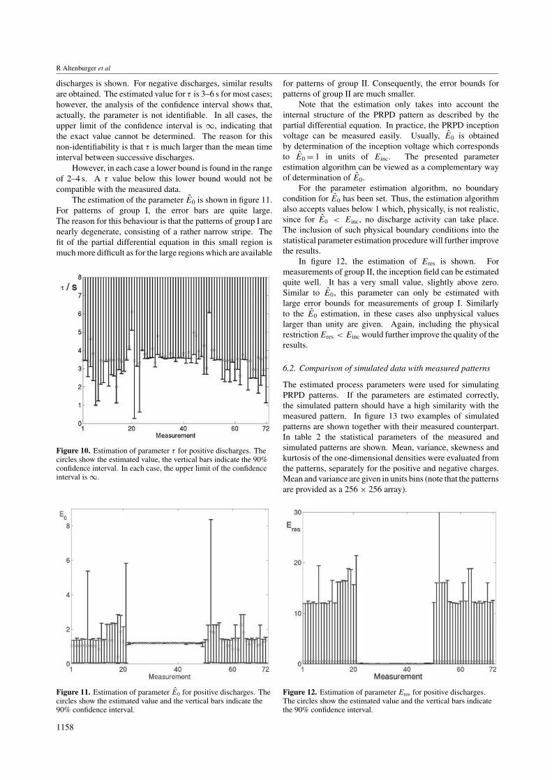
R Altenburger et al
discharges is shown. For negative discharges, similar results
are obtained. The estimated value for τ is 3–6 s for most cases;
however, the analysis of the confidence interval shows that,
actually, the parameter is not identifiable. In all cases, the
upper limit of the confidence interval is ∞, indicating that
the exact value cannot be determined. The reason for this
non-identifiability is that τ is much larger than the mean time
interval between successive discharges.
However, in each case a lower bound is found in the range
of 2–4 s. A τ value below this lower bound would not be
compatible with the measured data.
The estimation of the parameter E0 is shown in figure 11.
For patterns of group I, the error bars are quite large.
The reason for this behaviour is that the patterns of group I are
nearly degenerate, consisting of a rather narrow stripe. The
fit of the partial differential equation in this small region is
much more difficult as for the large regions which are available
Figure 10. Estimation of parameter τ for positive discharges. Thecircles show the estimated value, the vertical bars indicate the 90%confidence interval. In each case, the upper limit of the confidenceinterval is ∞.
Figure 11. Estimation of parameter E0 for positive discharges. Thecircles show the estimated value and the vertical bars indicate the90% confidence interval.
for patterns of group II. Consequently, the error bounds for
patterns of group II are much smaller.
Note that the estimation only takes into account the
internal structure of the PRPD pattern as described by the
partial differential equation. In practice, the PRPD inception
voltage can be measured easily. Usually, E0 is obtained
by determination of the inception voltage which corresponds
to E0 = 1 in units of Einc. The presented parameter
estimation algorithm can be viewed as a complementary way
of determination of E0.
For the parameter estimation algorithm, no boundary
condition for E0 has been set. Thus, the estimation algorithm
also accepts values below 1 which, physically, is not realistic,
since for E0 < Einc, no discharge activity can take place.
The inclusion of such physical boundary conditions into the
statistical parameter estimation procedure will further improve
the results.
In figure 12, the estimation of Eres is shown. For
measurements of group II, the inception field can be estimated
quite well. It has a very small value, slightly above zero.
Similar to E0, this parameter can only be estimated with
large error bounds for measurements of group I. Similarly
to the E0 estimation, in these cases also unphysical values
larger than unity are given. Again, including the physical
restriction Eres < Einc would further improve the quality of the
results.
6.2. Comparison of simulated data with measured patterns
The estimated process parameters were used for simulating
PRPD patterns. If the parameters are estimated correctly,
the simulated pattern should have a high similarity with the
measured pattern. In figure 13 two examples of simulated
patterns are shown together with their measured counterpart.
In table 2 the statistical parameters of the measured and
simulated patterns are shown. Mean, variance, skewness and
kurtosis of the one-dimensional densities were evaluated from
the patterns, separately for the positive and negative charges.
Mean and variance are given in units bins (note that the patterns
are provided as a 256 × 256 array).
Figure 12. Estimation of parameter Eres for positive discharges.The circles show the estimated value and the vertical bars indicatethe 90% confidence interval.
1158
Analysis of PRPD patterns of voids
Simulated Simulated
Measured Measured
C
D
BA
Figure 13. Simulated data with parameter sets from estimation in comparison with corresponding measured patterns.
Table 2. Statistical parameters of the measured and re-simulated patterns shown in figure 13.
Mean Variance Skewness Kurtosis
Meas. Simul. Meas. Simul. Meas. Simul. Meas. Simul.
Void0021qpos 38.571 43.646 1.976 0.976 0.872 0.074 −0.242 0.06tpos 24.793 22.097 306.797 228.514 0.460 0.371 −0.728 −0.661qneg −46.836 −44.395 14.581 2.962 −0.345 −1.292 0.011 3.375tneg 153.26 150.208 191.491 213.61 0.516 0.449 −0.188 −0.547
Void0030qpos 57.558 57.965 208.02 185.375 0.810 0.967 −0.273 −0.081tpos 30.762 34.144 624.147 621.526 0.948 0.466 0.119 −0.546qneg −65.409 −65.167 153.835 220.135 −0.500 −0.353 −0.792 −1.059tneg 189.86 195.458 498.107 1085.64 −0.064 −0.106 −0.358 −0.918
It can be seen that the simulated patterns show a high
similarity with the measured patterns. Typical pattern features
are reproduced correctly. Examples are:
• the increased point density at the upper edge of the pattern,
especially at ϕ ≈ 0 (region A in figure 13);
• the occurrence of a second point accumulation for small
positive discharges at ϕ ≈ π/2 (region B in figure 13);
• the occurrence of two adjoining point clowds for negative
discharges (region C in figure 13). In the simulated
pattern, the separation between these two clouds is less
pronounced than in the measured pattern, but it is clearly
present.
• the lack of discharges in region D in figure 13. This lack
is only present for negative discharges.
Note that the different pattern structure for positive and
negative discharges is reproduced correctly. This is a very
strong result due to the following reason. For the parameter
estimation the two half-waves have been analysed separately,
leading to different PD parameters for positive and negative
discharges. No explicit mutual coupling between the two
discharge polarities have been taken into account. The only
information which is exploited for the parameter estimation is
the internal structure of the point pattern in a predefined region
of the PRPD pattern.
In reality, however, the positive and negative discharges
are coupled. The discharge behaviour in the positive half-wave
has direct consequences for the discharge behaviour in the
negative half-wave, and vice versa. This mutual coupling is not
used for the parameter estimation. However, when simulating
patterns with the estimated parameter values, this coupling
is taken into account. For patterns with a difference between
negative and positive discharges it is therefore far from being an
automatism that simulation of the PD process (with separately
estimated parameters) lead to PRPD patterns with the correct
structure.
In figure 13, the counts per cycle for positive and negative
discharges are displayed for the measured patterns as well as
1159
R Altenburger et al
for the simulated ones. The simulations have a slightly higher
number of discharges than the measured patterns. The reason
for this systematic deviation is not yet clear. A possible reason
could be the dead times of the PD measuring system leading to
a number of discharges which is systematically too low. This
assumption is supported by the observation that the deviation
is larger for pattern with a high values of counts per cycle.
It must be stressed that the values of counts per cycle
for the measured patterns are not an input of the parameter
estimation algorithm. The parameter estimation is based on
the master (equation (13) or (16)) which is is a differential
equation for the point density which is independent on the
absolute pattern density. Consequently, the estimation of the
parameters is based solely on the relative temporal change of
the point density within the pattern, not on the absolute value
of the point density. Taking this into account, the reproduction
of the point density (measured by the counts per cycle) within
an error range of only some 10% is a validation of the model
and the presented parameter estimation procedure.
However, some properties of the pattern are not
reproduced by the simulation. For example, the step in the
horizontal stripe of figure 13 does not appear in the simulation.
Instead, the simulation yields a horizontal stripe without a
charge step.
Regarding the statistical parameters in table 2, there
are some significant differences between the original and
the simulated patterns, especially for the pattern of group I
(void0012, left patterns in figure 13). For example, the
variance of the negative charge distribution for void0012 is
much too low in the simulated pattern. For skewness and
kurtosis occasionally large deviations arise.
The reason for these deviations probably is originated
in too simplified a model for the discharge process. Note
that the description of the discharge process with only two
physical parameters c and τ (the other parameters E0 and Eres
are, striktly speaking, not discharge parameters but instead
describe the external field) is a very crude approximation to
the true complexity of the physical processes involved. For
example, the physical model for void discharges developed
in [5, 26] is much more complicated than the used simple
model of [8]. Additionally, in the used parameter extraction
algorithm, the first electron supply has been assumed to be
constant ignoring first electron supply by surface electrons.
Therefore, is expected that the model cannot capture all details
of the pattern.
In contrast, actually it is very surprising that the underlying
simple model is able to describe so much detail of the measured
PRPD pattern, and that the parameter estimation procedure
based on this model works that well. In spite of its simplicity,
the model seems to describe correctly the main features of the
physical process for the examined data.
7. Discussion
This section contains some additional remarks on the presented
parameter estimation algorithm.
The approach allows one to extract information about
the physical parameters of a PD without a simulation of the
discharge process. To the knowlegde of the authors, there is no
similar approach available in literature. Usually, the physical
parameters of a PD process are estimated by simulation of
the process according to a physical model, comparing the
output of the simulation with measured data, and changing
the parameters until a match between simulated and measured
data is obtained. The present method, in contrast, is able
to directly estimate the physical process parameters by data
analysis. Moreover, error bounds can be given easily, which
is very difficult with a trial-and-error parameter estimation
method using simulation.
Compared with other data analyis methods used, like the
extraction of statistical properties such as mean, skewness,
etc, from measured PRPD pattern, the proposed method is
superior since it renders physical information about the PD
process which describes the nature of the process much better
than in terms of simple descriptive statistical numbers. As
has been shown in section 6, a change of one of the physical
parameters (availability of first electrons) leads to patterns with
a completely different structure. The analysis of the physical
parameters shows clearly that only this one parameter has
changed while the others remain constant. Another example is
the comparison of patterns of the same PD defect at different
applied voltages. Here the usual statistical measures are
different. However, the physics of the discharge process,
described by the parameters c and τ , remains the same, which
can be clearly revealed by the proposed method.
It must be stressed that, as for all physical models, the
parameter estimates only make sense if the model for the
discharge process is correct. The presented algorithm is based
on a fairly simple model with only few physical parameters.
As mentioned above, it is to be expected that there may be
situations where the model may be too simplified and thus
inappropriate. For example, effects like shielding due to
conductivity of cavity walls or multi-PD phenomena in the
same cavity cannot be described. The great advantage of the
model developed in [8] is that it allows a direct parameter
estimation as described in this paper. This is in contrast to
more detailed physical models like those used in [5, 26] which
describe the process more accurately but render no possibility
to directly extract the parameter values from measured data.
Thus, the authors hope that the used simplified model together
with the possibility to extract the parameters directly from
the data helps to get a better understanding of measured PD
phenomena, even if the model can only be an approximative
one. Note, however, that the aim of this paper is not to prove
the validity of the underlying model assumption but to describe
an approach for physical parameter extraction based on the
stochastic model description of [8].
The presented algorithm does not make use of the absolute
charge value but is based on the temporal change of the pattern
as expressed in equation (6). This independence of the
absolute charge means that, for the parameter estimation, the
electromagnetic coupling between PD source and PD sensor
need not be known. This is very advantageous in practice
where the position of the PD source often is not known exactly.
The holographic property of the PRPD pattern is fully
exploited by the presented parameter estimation. For the
parameter estimation, it is not necessary to use the whole
pattern but a restriction to a part of the pattern is possible.
This large freedom in choosing the analysis region has a huge
impact on the practical usefulness of the approach. In practice,
1160
Analysis of PRPD patterns of voids
measured PDs are often corrupted by noise sources, or many
PD sources are active at the same time, leading to overlapping
patterns. In these cases, traditional PD analysis methods fail.
For example, deriving statistical parameters like skewness or
kurtosis makes no sense if more than one PD source is active, or
if a strong noise source is present. Our approach, in contrast,
can easily deal with noise and multi-source patterns as long
as there are regions in the pattern which can be assigned to a
single defect. It is possible to restrict the parameter estimation
to exactly this region and extract information on this single PD
defect.
The parameter estimation method has been presented for
the case of void discharges with a constant supply of first
electrons. It has been shown in section 3.6 that the approach
can be extended to the case of first electron supply by trapped
surface charges. In principle, the same idea of parameter
estimation could also be applied to other kinds of PD sources
as well, e.g. corona discharges or surface discharges. This
is possible since these discharges are described by the same
kind of master equation [8]. The only difference is the relation
between the field change �E and the measured charge q of
the discharge which is linear for void discharges and takes the
form of a power law for other discharges [8]:
q = −γ (�E)α.
An adoption of the presented method to other discharge types
would therefore be possible. Moreover, the exponent α could
be treated as an additional parameter which could be estimated
analogously to the others. The resulting algorithm would then
not only yield the physical parameters as described above, but
also additional information on the type of the discharge. This
could be used as a means for classification of PD sources based
on physical parameters.
8. Conclusion
In this paper, a novel method for estimation of physical
discharge parameters for PDs in voids has been presented.
The method is based on a recently developed framework for
modelling a PD process as a stochastic process governed by a
master equation.
The parameter estimation algorithm makes use of the
specific form of this master equation. By using a ML
approach, the parameters can be estimated. Furthermore,
error bounds for the parameter estimates can be given. With
this method a compact description of a PD pattern in terms
of the physical parameters governing the discharge process
is possible. In contrast to purely descriptive statistical
parameters, the physical parameters can be interpreted in terms
of discharge physics.
The method has been tested by application to different
simulated PRPD patterns. It has also been successfully applied
to measured data of a series of PRPD measurements of a void
in epoxy resin subjected to varying UV radiation. The change
of first electron availability is reflected by a clear change of the
corresponding physical parameter c.
The parameter estimation method works on a contiguous
region of the PRPD pattern which may be only a small part
of the actually measured pattern. This holographic property
of the method allows the application of the method even on
patterns with are strongly corrupted by noise, as long as there
are regions in the q–t space which are essentially free of noise.
For patterns with several active PD defects, the single defects
can be analysed separately as long as they are separated, at
least partly, within the pattern. This is not possible with usual
pattern analysis techniques.
Acknowledgment
We are very grateful to Power Diagnostics GmbH for their
permission to use their data for testing the parameter extraction
method.
Appendix A. Transformation from (Ei; t) to (x, t)
For regions {(Ei; t)|c(Ei; t) > 0} and under the assumption
that f has the form given in equation (5), the master
equation describing the process dynamics has the form (see
equation (13)):
∂
∂tp(Ei; t) =
(
1
τ− c
)
p(Ei; t) +Ei
τ
∂
∂Ei
(p(Ei; t)). (27)
We consider the transformation Ei → x = Eiet/τ .
Normalization of the probability density has to be fulfilled
at every time t , thus we have
p(x; t) = p(Ei(x); t) ·dEi
dx= p(Ei; t)e−t/τ . (28)
The temporal derivative of p(x; t) is given by
dp(x; t)
dt=
∂p
∂x
∂x
∂t+
∂p
∂t=
x
τ
∂p
∂x+
∂p
∂t
The LHS of equation (27) now reads
d
dtp(Ei; t) =
d
dt(p(x; t)et/τ ) = et/τ
(
x
τ
∂p
∂x+
∂p
∂t
)
+p
τet/τ .
Withd
dEi
=dx
dEi
d
dx= et/τ d
dx,
the RHS of equation (27) takes the form
(
1
τ− c
)
p(x; t)et/τ +xe−t/τ
τet/τ d
dxp(x; t)et/τ .
Comparing LHS and RHS, most of the terms cancel out,
leading to∂p(x; t)
∂t= −c(x, t)p(x; t).
Appendix B. Estimation of A(x)
Given a transformed PRPD pattern in the x–t space, each
measured PD event corresponds to one point of this pattern.
From theory (see appendix A) it is known that the process has
the probability density
p(x; t) = A(x)e−ct , (29)
1161
R Altenburger et al
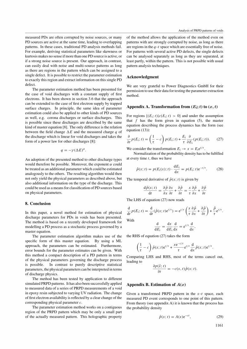
where A(x) is an initial distribution which is not known butmust be estimated from the data. The above equation is validonly for a contiguous region for which c > 0 (see section 3.2).While this region has generally a simple form in the q–t spaceof the original pattern, it can have a complicated form in thex–t space (see figure 14).
The measured PD pattern in the x–t space has a pointdensity which is given by
pd(x, t) = c(x, t)p(x, t). (30)
The task is to estimate the distribution A(x) such thatequation (30) is consistent with the measured data.
By integrating pd(x, t) over t one gets (see figure 14)∫ T
0
pd(x, t) dt =
∫ b
a
cp(x; t) dt
= cA(x)
∫ b
a
e−ct dt
= A(x)(e−cb − e−ca),
where a and b are the interval boundaries for the region wherec > 0. Thus
A(x) =
∫ T
0pd(x, t) dt
e−cb − e−ca.
Thus, in principle, the density A(x) can be estimated bysumming all PD events along a horizontal line in the x–t spaceand dividing by the factor (e−cb − e−ca). In practice, however,the resulting density Aest(x) is very peaked, especially whenthe pattern consists of few points. Therefore, the calculatedestimated density is additionally smoothed with a smoothingkernel. The resulting estimator for the initial distribution A(x)
can thus be interpreted as a kernel estimator.In order to yield a valid probability density, the resulting
estimated density
pest(x, t) = Aest(x)e−ct
is normalized in order to get∫
t
∫
x
pest(x, t) dx dt = 1,
where the integration extends over the whole considered regionof the x–t space.
a b t
Figure 14. Estimation of the initial distribution A(x) from the data.For a given x, the value of the initial distribution A(x) can be derivedfrom the data by integrating all PD events along a horizontal line.
References
[1] Devins J C 1984 The physics of partial discharges in soliddielectrics IEEE Trans. Electric. Insul. 19 475–95
[2] van Brunt R J and Kulkarni S V 1990 Stochastic properties ofTrichel-pulse corona: a non-Markovian random pointprocess Phys. Rev. A 42 4908–32
[3] van Brunt R J 1991 Stochastic properties of partial-dischargephenomena IEEE Trans. Electric. Insul. 26 902–48
[4] Fromm U and Gulski E 1994 Statistical behaviour of internalpartial discharges at DC voltage Prod. 4th Intern. Conf. onProperties and Applications of Dielectric Materials(Brisbane, Australia, 1994) paper 6230
[5] Niemeyer L 1995 A generalized approach to partial dischargemodeling IEEE Trans. Diel. Electric Insul. 2 510–28
[6] Hoof M and Patsch R 1997 A physical model: describing thenature of partial discharge pulse sequence ICPADM 97(Seoul, Korea 1997) pp 283–6
[7] Patsch R and Hoof M 1998 Physical modelling of partialdischarge patterns IEEE 6th Intern. Conf. on Conductionand Breakdown in Solids ICSD’98 (Vasteras Sweden)114–8
[8] Heitz C 1999 A generalized model for partial dischargeprocesses based on a stochastic process approach J. Phys. D32 1012–23
[9] Okamoto T, Kaot T, Yokomizu Y and Suzuoki Y 2001 PDcharactaristics as a stochastic process and its integralequation under sinusoidal voltage IEEE Trans. Diel.Electric. Insul. 8 82–90
[10] 1969 Recognition of discharges Electra (CIGRE) No 11,pp 61–98
[11] Nattrass D A 1988 Partial discharge measurement andinterpretation IEEE Electric. Insul. Magazine 4 10–23
[12] Laurent C and Mayoux C 1992 Partial discharge: XI.Limitations to PD as a diagnostic for deterioration andremaining life IEEE Electric. Insul. Magazine 8 14-17
[13] Satish L and Gururaj B I 1993 Use of hidden Markov modelsfor partial discharge pattern classification IEEE Trans.Electric Insul. 28 172–82
[14] Hikita M, Kato T and Okubo H 1994 Partial dischargemeasurements in SF6 and air using phase-resolvedpulse-height analysis IEEE Trans. Diel. Electric. Insul. 1267–83
[15] Gulski E 1995 Digital analysis of partial discharges IEEETrans. Diel. Electric. Insul. 2 822–37
[16] Cachin C and Wiesmann H J 1995 PD recognition withknowledge-based preprocessing and neural networks IEEETrans. Diel. Electric. Insul. 2 578–89
[17] Ziomek W, Schlemper H-D and Feser K 1996 Computer aidedrecognition of defects in GIS Proc. IEEE Int. Symp. onElectric. Insul. (Montreal) pp 91–4
[18] Huecker T 1997 UHF partial discharge expert systemdiagnosis Proc. 10th Int. Symp. on High voltageEngineering pp 259–62
[19] Contin A, Montanari G C and Ferraro C 2000 PD sourcerecognition by Weibull processing of pulse heightdistributions IEEE Trans. Diel. Electric. Insul. 7 48–58
[20] Candela R, Mirel G and Schifani R 2000 PD recognition bymeans of statistical and fractal parameters and a neuralnetwork IEEE Trans. Diel. Electric. Insul. 7 87–94
[21] Salama M M A and Bartniaks R 2000 Fuzzy logic Applied toPD pattern classification IEEE Trans. Diel. Electric. Insul. 7118–23
[22] Hikita M, Yamada K, Nakamura A, Mizutani T, Oohasi A andIeda M 1990 Measurements of partial discharges bycomputer and analysis of partial discharge distribution bythe Monte Carlo method IEEE Trans. Electric. Insul. 25453–68
[23] Niemeyer L, Fruth B and Kugel H 1991 Phase resolved partialdischarge measurements in particle contaminated SF6
insulation Geasous Dielectrics vol VI, edL G Christophorou and I Sauers (New York: Plenum)
1162
Analysis of PRPD patterns of voids
[24] Niemeyer L, Fruth B and Gutfleisch F 1991 Simulation ofpartial discharges in insulation systems 7th ISH paper 71.05
[25] Niemeyer L 1993 Interpretation of PD measurements in GISProc. 8th Int. Symp. on High Voltage Engineeringpaper 68.04
[26] Gutfleisch F and Niemeyer L 1995 Measurement andsimulation of PD in epoxy voids IEEE Trans. Diel Electric.Insul. 2 729–43
[27] Suzuoki S Y, Komori F and Mizutani T 1996 Partial dischargesdue to electrical treeing in polymers: phase-resolved andtime-sequence observation and analysis J. Phys. D: Appl.Phys. 29 2922–31
[28] Morshuis P and Niemeyer L 1996 Measurement andsimulation of discharge induced ageing processes in voidsProc. CEIPD (San Francisco)
[29] Schifani R, Romano P and Candela R 2001 On PDmechanisms at high temperature in voids included in anepoxy resin IEEE Trans. Diel Electric. Insul. 8 589–97
[30] Gardiner C W 1985 Handbook of Stochastic Methods(Springer Series in Syergetics vol 13) (Berlin: Springer)
[31] van Kampen N G 1992 Stochastic Processes in Physics andChemistry
[32] Silverman B W 1986 Density Estimation for Statistics andData Analysis (Chapman and Hall: London)
[33] Press W H, Flannery B P, Saul S A and Vetterling W T 1992Numerical Recipes (London: Cambridge UniversityPress)
[34] Efron B and Tibshirani R J 1998 An Introduction to theBootstrap (New York: Chapman and Hall)
[35] http://www.pd-systems.com/[36] Gross D W and Fruth B A 1998 Characteristics of phase
resolved partial discharge patterns in spherical voidsCEIDP98
[37] Pedersen A, Crichton G C and McAllister I W 1995 Thefunctional relations between partial discharges and inducedcharges IEEE Trans. Diel. Electric. Insul. 2535–43
[38] Crichton G C, Karlsson P W and Pedersen A 1989 Partialdischarges in ellipsoid and spherical voids IEEE Trans.Electric. Insul. 24 335–42
1163
Recommended