SEA - Practical Application of Science
Volume V, Issue 15 (3 / 2017)
331
Florin POPESCU Doctoral School - Entrepreneurship, Business Engineering & Management
University “Politehnica” of Bucharest, Romania
ANALYSIS OF FORECASTING METHODS FROM THE POINT OF
VIEW OF EARLY WARNING CONCEPT IN PROJECT
MANAGEMENT
Review Article
Keywords Early warning,
Forecasting methods, Project management
JEL Classification L00
Abstract Early warning system (EWS) based on a reliable forecasting process has become a critical component of the management of large complex industrial projects in the globalized transnational environment. The purpose of this research is to critically analyze the forecasting methods from the point of view of early warning, choosing those useful for the construction of EWS. This research addresses complementary techniques, using Bayesian Networks, which addresses both uncertainties and causality in project planning and execution, with the goal of generating early warning signals for project managers. Even though Bayesian networks have been widely used in a range of decision-support applications, their application as early warning systems for project management is still new.
SEA - Practical Application of Science
Volume V, Issue 15 (3 / 2017)
332
INTRODUCTION
In the today's volatile economic environment, risk
management retains its important position on the
agenda of each organization or project. Today's big
organizations and projects are still struggling with
the changes to the post-recession economy, where
investors are looking for a thorough risk
assessment before investing. Risk management in
projects has been and is still being debated
vigorously, project managers realizing the
importance of predictability of external factors
correlated with the internal process. In this context,
risk and uncertainty management is again a trend,
many risk identification/evaluation tools being
developed to allow management teams to identify
and assess the risks that their organizations face
before produce negative effects. Planning and
execution of complex industrial projects inevitably
involve uncertainties, vulnerabilities and risks both
internally and externally. Basic inputs (time, costs,
and resources planned for each activity) are not
deterministic and are affected by various sources of
uncertainties. Moreover, there is a causal
relationship between these sources of uncertainties
and the project parameters which is not modeled by
the traditional project planning techniques. Early
warning of risks and uncertainties should be seen as
an essential component of the management of any
complex large-scale project to incorporate
uncertainties from the early project planning stage,
despite the different approaches, methods and tools
available. Most current techniques for addressing
risk and uncertainty in project planning and
execution (simulation techniques) are often event-
oriented and attempt to model the impact of
possible threats to project performance. They
ignore the causal relationship between sources of
uncertainty and project parameter and,
consequently, advanced techniques are needed to
capture different aspects of uncertainties in
projects. EWS new approach that makes it possible
to include risk, uncertainties and causality in the
planning and execution of projects by:
• identification of different sources of uncertainty
and their use for informing the project staff from
the planning stage;
• exposing the uncertainties about the completion
time for each activity and for the whole project
with full probability distributions;
• using the analysis "What if?" to identify the level
of resources needed, taking into account
constraints such as, for example, a certain
completion time;
• awareness of the veracity of data so that forecasts
become more relevant and accurate.
UNCERTAINTIES AND RISKS IN PROJECT
MANAGEMENT
When a decision is taken under risk conditions, it
involves knowing the assumed risk, ie knowledge
of the likelihood of occurrence of the risk. In the
case of a decision taken under uncertainty, risks are
not known, although they are assumed. For
example, an individual who goes to work on the
morning is looking out the window and sees it is
cloudy but not raining, which makes him take his
umbrella considering it may be raining during the
day. This is a decision under uncertain conditions.
If he watched the weather, he could see that there
was an 80% chance of it raining that day, which
would have made him surely take his umbrella, in
which case he would have taken a risk-taking
decision. In the example above, it can be noticed
that the decision under uncertainty conditions is
based more on intuition than on substantiated
information, so we can say that if the probability of
occurrence of an event is known it is possible to
make more correct judgments under risk conditions
than under conditions of uncertainty.
The possibility of something undesirable
happens is referred to as "risk" (Rowe, 1977).
Typically, critical words in a sentence describing
the nature of the risks are "possibility" and
"unwanted". In the literature, several parallel
definitions of risk coexist. Rescher, (1983) defined
risk as an uncertain situation with possible negative
outcomes. Williams et al., 1998, said that risk can
generally be defined as a collection of pairs
between probabilities (L) and results (O):
Risk = {(L1O1), (L2O2), (L3O3),.... (LnOn)}
The pattern of pairs distribution formed by
probabilities and outcomes is called a risk profile
(Avyub, 2003). Risk definitions must also have a
time dimension or a certain time horizon, as well as
a specific perspective or view that defines the unit
of analysis (eg limits, etc.). International
Organization for Standardization (ISO 2002)
defines two of the essential components of risk: the
losses and the uncertainty of their occurrence (the
probability of a risky event).
PMBOK 2004 sees risk management as a key
area: "... as those processes involved in identifying,
analyzing and responding to project riskS,
including maximizing positive event outcomes and
minimizing the consequences of adverse events."
Ward and Chapman (2003) argue that the central
element of risks management has a narrow focus on
managing uncertainties in projects, which they
believe is due to the fact that the term "risk" has
become associated with "events", rather than
general sources of significant uncertainties. The
most obvious area of uncertainty is in estimating
the duration for a particular activity. The difficulty
in this estimate comes from a lack of knowledge of
SEA - Practical Application of Science
Volume V, Issue 15 (3 / 2017)
333
what is involved, rather than the uncertain
consequences of potential threats or opportunities.
From, both, specialized literature and management
practice on risk management, this research
synthesizes “roots” of uncertainties as well as the
most important internal or external factors that
could have a major impact on the performance of
large complex industrial projects:
“Roots” of uncertainty could be represented by the
one or more of the following:
• the level of resources needed and available;
• compromise between resources and time;
• possible occurrence of uncertain events;
• causality factors and interdependencies,
including common occasional factors affecting
multiple activities (such as organizational
problems);
• lack of experience and use of subjective data
than objective ones;
• incomplete or inaccurate data, or total data loss.
External risk factors and internal factors could
affect the results of large complex industrial
projects:
➢ External risks
• Interruption/lack of critical infrastructures
(physical and virtual) - the backbone of any
complex project;
• High competition/complementary projects;
• Exchange rate risk;
• The sudden change in the price of raw
materials;
• Interruptions of the supply chains;
• Regulatory risks (national and/or regional);
• Local and/or regional economic instability;
• Access to credit.
➢ Internal factors
• Complexity and size of the project; • Time pressure in project execution; • Volume of workload; • Productivity variation; • The level of dependence on key people; • Lack of key technologies; • Degree of maturity of technological
development; • Level of communication in the project team; • Level of change control; • Rate of defects.
As Ward and Chapman (2003) have argued,
management of project uncertainties should not
only be reduced to managing perceived threats, but
also to their opportunities and implications.
Appropriate management of uncertainties should
include: identifying different sources of
uncertainty, understanding its origins and then
managing it with desired or unwanted implications.
To capture uncertainties in projects, it needs to go
beyond the variability and availability of data. It
has to address ambiguities and incorporate
structures and knowledge "(Chapman and Wards,
2000). In order to properly measure and analyze
uncertainties, relationships between the trigger
(source), risks and their impact (consequences)
must be shaped.
EVALUATION CRITERIA FOR
FORECASTING METHODS IN PROJECT
MANAGEMENT FROM THE POINT OF
VIEW OF GENERATING EARLY WARNING
SIGNALS
In project management, various forecasting
methods are used to provide confidence estimates
of success in achieving the final goals. Each project
is unique in its objectives, in its plan to achieve its
objectives and in the actual progress guided by the
established plan. By default, the performance of the
forecasting methods varies from one project to
another depending on the project's specific
situations. Even with the same information
available, some projects may be more difficult to
predict for some methods than others because of
the individual features of each project. Therefore, it
was the challenge of this research, namely to
evaluate the performance of the different methods
and compare them objectively.
Therefore, setting evaluation criteria is a crucial
first step in evaluating and comparing forecasting
methods. Correct understanding of the criteria is
essential for the correct interpretation of the results.
In a traditional project control system, the forecasts
are evaluated and compared to whether the
deviation from the planned performance is
significant or not. In the view of this research, the
performance of predictive methods through early
warning has to be measured in terms of:
• accuracy;
• timeliness;
• reliability.
An ideal case would be one in which the three
above criteria are maximized simultaneously.
However, in most situations, compromises between
these factors are required to be in line with the
management strategy or project priorities. The
main purpose of the assessment framework is to
analyze different forecasting methods with regard
to prediction accuracy, alertness, and the reliability
of the warnings they generate. The novelty,
confidence and reliability of a method should be
evaluated on the basis of early warning warnings
instead of the average of precision over a period of
time.
In the predictive literature, precision is known as
the most commonly used criterion, both among
practitioners and researchers (Carbone and
Armstrong 1982). Vanhoucke and Vandevoorde
(2006) state that "the accuracy of forecasts based
on statistical error measures should not be confused
SEA - Practical Application of Science
Volume V, Issue 15 (3 / 2017)
334
with the early warning capability of forecasting
methods."
The current alert signals have also been recognized
as a desirable feature of project performance
forecasts (Teicholz 1993) and serve as an important
criterion for assessing their performance
(Vanhoucke and Vandevoorde 2006). Confidence
in warnings is also an important factor, especially
for practitioners, which needs to be considered in
the evaluation of forecasting methods.
The ultimate goal of analyzing forecasting methods
is to select them for different phases of the project
as inputs for SHAT construction. Therefore, an
early warning system based on predictive
predictions becomes an essential part of pro-active
project management. With an early trusted warning
system, project teams may be able to decide when
further attention is needed to detect some early
symptoms or indicators of future problems.
EVALUATING THE PERFORMANCE OF
FORECASTING METHODS BASED ON
EVALUATION CRITERIA THROUGH THE
"EARLY WARNING" APPROACH
The project performance forecast is a complex task
depending on the project manager's interest and
abilities, the type of project, the size and complexity
of the project, as well as the strategy adopted and an
essential part of the decision-making process in the
industrial project management process carried out in
an environment characterized by volatility,
uncertainties and risks. A lot of forecasting methods are available in the
literature, but they are often avoided because they do
not contain appropriate tools and reliable data, but
also a high difficulty in addressing uncertainties and
risks in the external environment of projects. The
limitations of deterministic forecasting approaches
have been repeatedly addressed over the last decades
(Ang and Tang 1975, Barraza et al., 2004, Hertz
1979, Spooner 1974) and will be set out in the final
section of this research.
Criteria for classifying forecasting methods:
In the literature there are many classifications,
according to different criteria, as follows:
For example, Makridakis et. al. have classified the
forecasting methods into four broad groups:
• Subjective approaches;
• Causality or explanatory methods;
• Extrapolated methods (time series);
• Any combination of the three.
On the other hand, Al - Tabtabai and Diekmann,
1992, classified prognostic methods in:
• Econometric models;
• Time series models;
• Judicial models.
Having so many models encountered in the
literature, the ones listed above not being the only
ones, the choice of the right method was itself a
challenge for this research.
Some authors, such as Georgoff and Murdick
(1986), evaluated over 20 forecasting techniques and
models based on 16 criteria to provide a guide to
project managers for choosing the best techniques or
a combination of them.
In the view of this research, the evaluation of
prognosis methods and techniques, whether
deterministic, statistical or probabilistic, has been a
challenge. In the industrial project management
community, the most commonly used practices for
project performance prediction are the Earned Value
Method, Critical Path Method and Monte Carlo
simulation. They will be analyzed from a prism
Early warning signals that they can generate for
managers and project teams.
Earned Value Method
Earned Value concept has been used since the
1890s when early industrial age engineers wanted
to measure the performances of US factories. They
analyzed the "cost variation" correlated with
"earned standards" relative to "actual spending" to
determine the industrial performance of that time.
In 1962 that earned value concept was formally
introduced into US Navy projects as part of the
PERT/Costing methodology. In 1967, EVM was
promoted and adopted in the Department of
Defense of the United States of America, wishing
to be a valuable project management and control
system that interconnects the cost, schedule and
physical progress achieved by the project team. The
following sections provide an overview of the
basics of EVM, based on several books and
articles, among which the most cited are Anbari
(2003), Fleming & Koppelman (2006) and
Vanhoucke (2006).
In addition to the traditional EVM methods, this
section also integrates the concept of Earned
Schedule (ES), because this relatively recently
developed concept goes beyond certain traps and
limitations of EVM, especially on the duration of
the forecast. But first of all, it is considered
necessary to clarify the terminology associated with
the "earned value" because it is often misused and
abusive.
• Earned value (EV0 analysis is a quantitative
technique for evaluating project
performance and predicting the project's
final results based on comparing progress
with planned budget and current costs;
• Earned Value Management (EVM) -
integrated cost and value management is a
methodology used to control a project that is
based on work performance measurement
with a WBS (Work Breakdown Structure)
and includes an integrated program and
budget on the WBS project;

SEA - Practical Application of Science
Volume V, Issue 15 (3 / 2017)
335
• Earned Value Management System
(EVMS) - represent the processes,
procedures, tools and models used by an
organization to apply value-added
management.
One of the most important issues for a project
management team is to accurately estimate the time
and cost of completion. Was the primary aim of
this research to analyze at the same time whether
EVM can be used as an early warning tool for the
performance of the internal process that might be
useful for project managers to identify and manage
problems before they become a risk for their
execution.
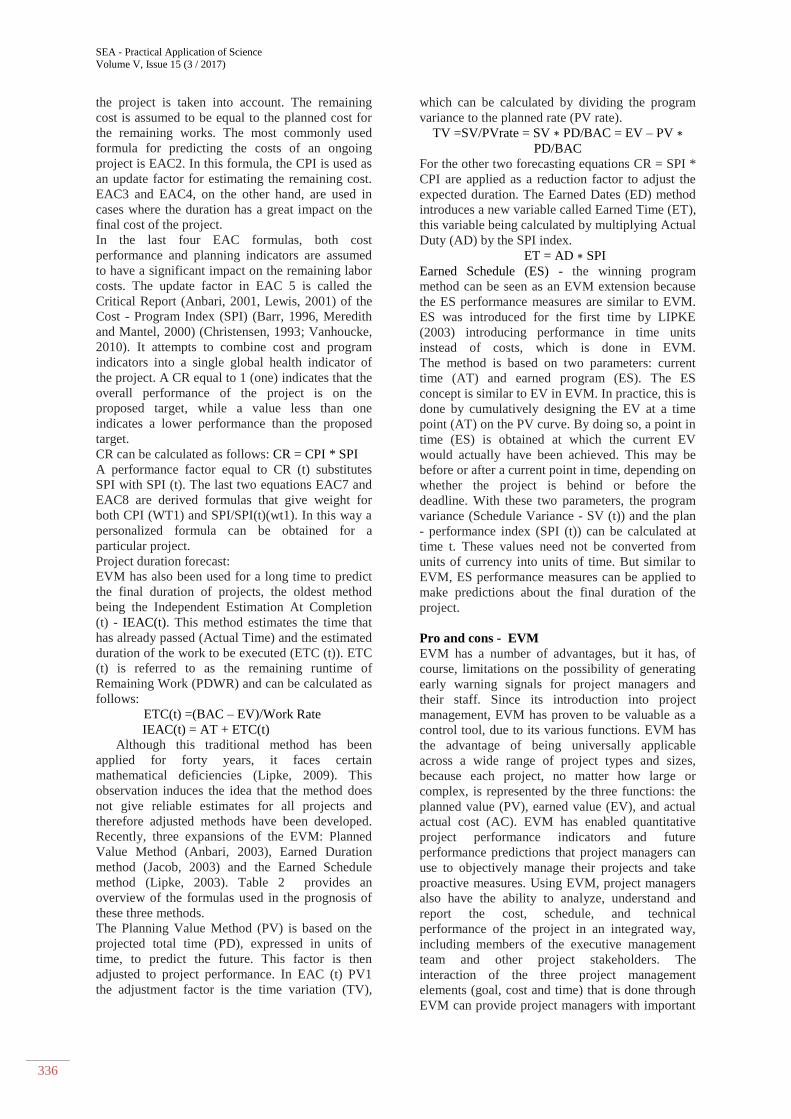
For this reason a brief introduction to key
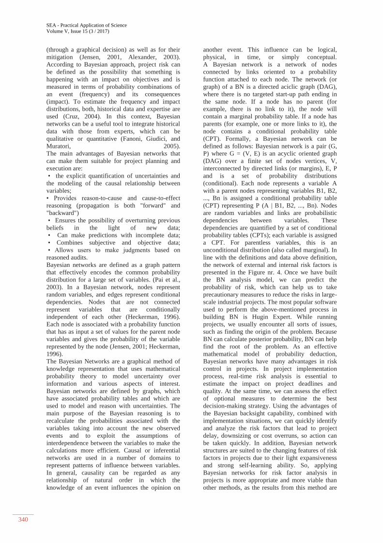
parameters used by EVM, as sketched in Fig.1 :
For the implementation of EVM and ES, a clear
project goal is needed, along with a budget and a
project runtime. Two project performance metrics
(cost and time) can be obtained during project
execution so that a comparison can be made
between reality and plan. Integrated cost and value
management uses three key parameters:
• Planned cost (PV), previously known as the
planned cost of work, is the amount that was
planned to be spent in accordance with the initial
plan.
• The actual cost (AC), formerly known as
Actual Cost for Work Performed (ACWP), is the
actual cost for all work that is executed at a given
point in time.
• Cost of Work Performed (BCWP) – the value
of an activity performed within a project is the cost
that the estimator associated with that activity when
the project budget was defined. The value obtained
is equal to the BAC (Budget at completion)
multiplied by the completed percentage (PC) at a
given point in time (EV = PC * BAC).
Measuring project performances:
If the three key parameters are properly recorded
over the life of the project, project managers may
be able to calculate two types of project
performance measurements. The first type of
performance measurement is the difference
between the current state of the project and the
basic one in monetary terms, called cost variation
(CV), which is used to track the project budget. A
negative/positive value shows that more/less
money was spent on the executed activities than
what was initially planned. The Time or Schedule
Variance is an indicator that gives project managers
a value showing whether the project is within
graphic or not. Positive or negative values mean
that the project is behind (before) the set schedule.
Another type of performance measurement of a
project is also calculated based on the three key
parameters described above. The indices are used
to show how well the project is performed.
Two types of indices can be distinguished:
• the first type of index is the cost
performance index (CPI), which
expresses the cost-effectiveness of the
executed works. An CPI of less or bigger
than to 1 (one) means that the project is
under or over the budget.
• the second index is the Schedule
Performance Index (SPI) that shows
whether the project is in the program set or
not. It is clear that clues and deviations are
interdependent. Variations can give a picture of
where the project is currently, while clues are used
to represent the performance of a project.
To sum up, deviations and clues can be calculated
as follows:
• Cost Variance is a value to be constantly updated
throughout the project = EV-AC;
• Cost Performance Index CPI - (Cost Performance
Index) = EV/AC;
• Deviation from program-SV- (Schedule
Variance) = EV –PV;
• Program performance-SPI(Schedule Performance
Index) = EV/PV.
Predictions on the evolution of a project using
the EVM method.
All performance metrics are designed to help
project managers to monitor project progress, both,
in terms of cost and schedule.
Cost forecast:
• Before the mathematical formulas are
displayed, some terms must be defined:
ETC - (Estimate To Complete) - estimated cost
for project completion;
• EAC - (Estimated At Completion) - the total
expected cost of project completion based on
performance up to the current date;
• BAC (Budget At Completion) - estimated
total budget estimate (including project
unforeseen).
In the case of the cost forecast, the emphasis is on
the estimate of the final cost of the project. EAC
consists of the actual cost (AC), the cost that has
been spent so far and an estimate of the cost of the
remaining works (ETC). In some specialized
works, the ETC is mentioned as find the Planned
Labor Cost of Work Remaining (PCWR). ETC can
be calculated using the following formula:
ETC = (BAC - EV)/performance factor.
There are several different formulas to calculate
EAC, depending on the performance factor that is
used to calculate the ETC (equation above).
Generally, eight forecast formulas are commonly
used and are accepted in managerial practice which
are synthetized within Table 1.
EAC1 assumes an update factor that is equal to
one. This means that in order to estimate the rest of
the project cost, no performance measurement of
SEA - Practical Application of Science
Volume V, Issue 15 (3 / 2017)
336
the project is taken into account. The remaining
cost is assumed to be equal to the planned cost for
the remaining works. The most commonly used
formula for predicting the costs of an ongoing
project is EAC2. In this formula, the CPI is used as
an update factor for estimating the remaining cost.
EAC3 and EAC4, on the other hand, are used in
cases where the duration has a great impact on the
final cost of the project.
In the last four EAC formulas, both cost
performance and planning indicators are assumed
to have a significant impact on the remaining labor
costs. The update factor in EAC 5 is called the
Critical Report (Anbari, 2001, Lewis, 2001) of the
Cost - Program Index (SPI) (Barr, 1996, Meredith
and Mantel, 2000) (Christensen, 1993; Vanhoucke,
2010). It attempts to combine cost and program
indicators into a single global health indicator of
the project. A CR equal to 1 (one) indicates that the
overall performance of the project is on the
proposed target, while a value less than one
indicates a lower performance than the proposed
target.
CR can be calculated as follows: CR = CPI * SPI
A performance factor equal to CR (t) substitutes
SPI with SPI (t). The last two equations EAC7 and
EAC8 are derived formulas that give weight for
both CPI (WT1) and SPI/SPI(t)(wt1). In this way a
personalized formula can be obtained for a
particular project.
Project duration forecast:
EVM has also been used for a long time to predict
the final duration of projects, the oldest method
being the Independent Estimation At Completion
(t) - IEAC(t). This method estimates the time that
has already passed (Actual Time) and the estimated
duration of the work to be executed (ETC (t)). ETC
(t) is referred to as the remaining runtime of
Remaining Work (PDWR) and can be calculated as
follows:
ETC(t) =(BAC – EV)/Work Rate
IEAC(t) = AT + ETC(t)
Although this traditional method has been
applied for forty years, it faces certain
mathematical deficiencies (Lipke, 2009). This
observation induces the idea that the method does
not give reliable estimates for all projects and
therefore adjusted methods have been developed.
Recently, three expansions of the EVM: Planned
Value Method (Anbari, 2003), Earned Duration
method (Jacob, 2003) and the Earned Schedule
method (Lipke, 2003). Table 2 provides an
overview of the formulas used in the prognosis of
these three methods.
The Planning Value Method (PV) is based on the
projected total time (PD), expressed in units of
time, to predict the future. This factor is then
adjusted to project performance. In EAC (t) PV1
the adjustment factor is the time variation (TV),
which can be calculated by dividing the program
variance to the planned rate (PV rate).
TV =SV/PVrate = SV ∗ PD/BAC = EV – PV ∗
PD/BAC
For the other two forecasting equations CR = SPI *
CPI are applied as a reduction factor to adjust the
expected duration. The Earned Dates (ED) method
introduces a new variable called Earned Time (ET),
this variable being calculated by multiplying Actual
Duty (AD) by the SPI index.
ET = AD ∗ SPI
Earned Schedule (ES) - the winning program
method can be seen as an EVM extension because
the ES performance measures are similar to EVM.
ES was introduced for the first time by LIPKE
(2003) introducing performance in time units
instead of costs, which is done in EVM.
The method is based on two parameters: current
time (AT) and earned program (ES). The ES
concept is similar to EV in EVM. In practice, this is
done by cumulatively designing the EV at a time
point (AT) on the PV curve. By doing so, a point in
time (ES) is obtained at which the current EV
would actually have been achieved. This may be
before or after a current point in time, depending on
whether the project is behind or before the
deadline. With these two parameters, the program
variance (Schedule Variance - SV (t)) and the plan
- performance index (SPI (t)) can be calculated at
time t. These values need not be converted from
units of currency into units of time. But similar to
EVM, ES performance measures can be applied to
make predictions about the final duration of the
project.
Pro and cons - EVM
EVM has a number of advantages, but it has, of
course, limitations on the possibility of generating
early warning signals for project managers and
their staff. Since its introduction into project
management, EVM has proven to be valuable as a
control tool, due to its various functions. EVM has
the advantage of being universally applicable
across a wide range of project types and sizes,
because each project, no matter how large or
complex, is represented by the three functions: the
planned value (PV), earned value (EV), and actual
actual cost (AC). EVM has enabled quantitative
project performance indicators and future
performance predictions that project managers can
use to objectively manage their projects and take
proactive measures. Using EVM, project managers
also have the ability to analyze, understand and
report the cost, schedule, and technical
performance of the project in an integrated way,
including members of the executive management
team and other project stakeholders. The
interaction of the three project management
elements (goal, cost and time) that is done through
EVM can provide project managers with important
SEA - Practical Application of Science
Volume V, Issue 15 (3 / 2017)
337
information about project performance and
progress during their lifecycle, which can help
project managers identify what to do to bring the
project back to the track.
EVM provides an overview of the current status of
the project and also provides insight into the future
of the project. As mentioned above, EVM focuses
mainly on project costs, which is why all
parameters and measures are expressed in monetary
units. On the one hand this has enabled EVM to be
very useful in presenting and analyzing project cost
performance, and on the other hand this has led to
some performance-plan performance abnormalities.
As Lipke mentioned, expressing plan-performance
measurements in monetary units instead of time
units makes it counterintuitive and difficult to
compare with other program indicators over time. From a practical point of view, project managers
should be more concerned about the timeliness and
reliability of the early warning signals generated by
this method than the accuracy in terms of statistical
errors. The ultimate goal of the forecast should be
to provide project managers with early warning
signals about success in achieving the project goals
(goal, budget, and completion date). Therefore,
alert signals should be accurate and, more
importantly, should be transmitted in due time.
One problem with the program pointers is that for a
project behind the program, at the completion of
the SV it returns back to zero, and the SPI equals
one unit. This may lead to biased conclusions
regarding the final duration of the project. The EVM method for a program's prognosis can
only be used to get trusted warnings after project
performance is stable. In practice, EVC EAC, EAC
= BAC/CPI, are recommended to be used only for
projects that are at least 20 percent achieved due to
instability inherent to CPI cumulative
measurements (Fleming and Koppelman 2006). On
the other hand, the predictive potential of EVM's
various prognosis formulas is still a controversial
problem among professionals. Some EVM experts
argue that ES data is not sufficient and should not
be invoked to predict the final completion date for
a project (Fleming and Koppelman 2006), while
others are struggling to find the appropriate
homologous formulas for cost forecasting in
projects (Lipke 2006, Vanhoucke and Vandevoorde
2006). Therefore, it can be concluded that the
winning method, which is known as the most
popular project management forecasting method,
provides reliable early warnings only after project
performance has stabilized, but it is very difficult to
know when this is achieved.
Critical Path Method (CPM)
In 1957, DuPont developed a new method for
project management to meet the need to shut down
a chemical plant for maintenance and then restart it
under operational conditions. Since the project was
extremely complex, a clear methodology had to be
set up and so DuPont creates Critical Path Method.
CPM is a deterministic technique that, by using a
dependency network between loads and
deterministic values for the given working time,
calculates the longest path in the network called the
"critical path." Activities are presented as nodes in
the network, and events that represent the
beginning or end of an activity are presented as
arcs or lines between these nodes. Such a graph
represents a meeting of arches and nodes in certain
relationships. Process activities are represented by
the arcs, while its events, meaning the significant
moments of time corresponding to the transition
from one activity to another, are represented by
nodes.
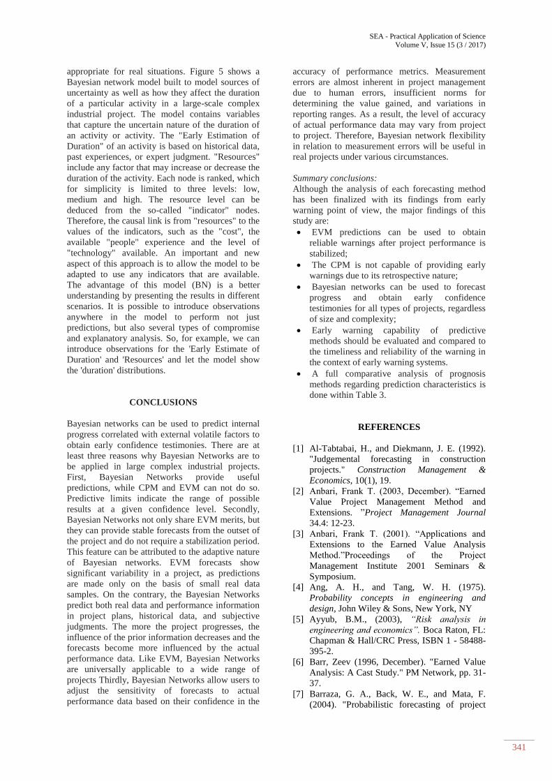
Generally speaking a graph is mathematically
defined as follows:
• Sets of X;
• Aplication Г:X → Р(X).
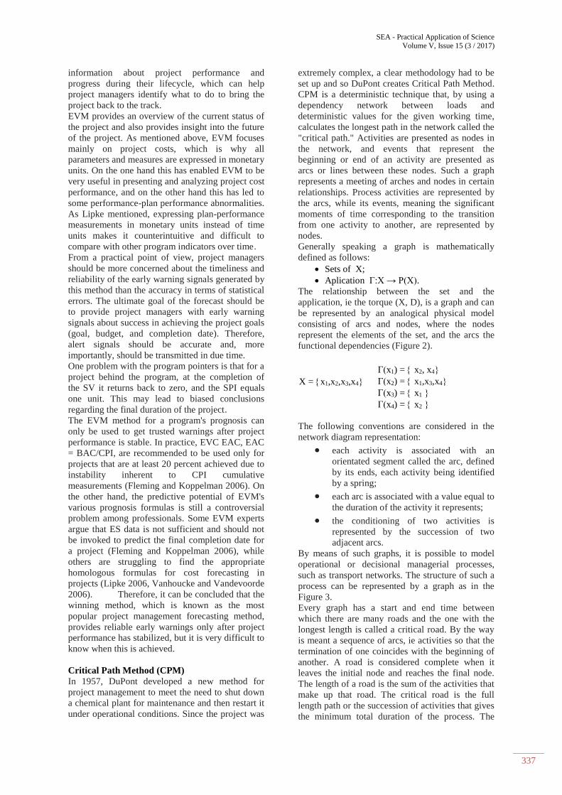
The relationship between the set and the
application, ie the torque (X, D), is a graph and can
be represented by an analogical physical model
consisting of arcs and nodes, where the nodes
represent the elements of the set, and the arcs the
functional dependencies (Figure 2).
The following conventions are considered in the
network diagram representation:
• each activity is associated with an
orientated segment called the arc, defined
by its ends, each activity being identified
by a spring;
• each arc is associated with a value equal to
the duration of the activity it represents;
• the conditioning of two activities is
represented by the succession of two
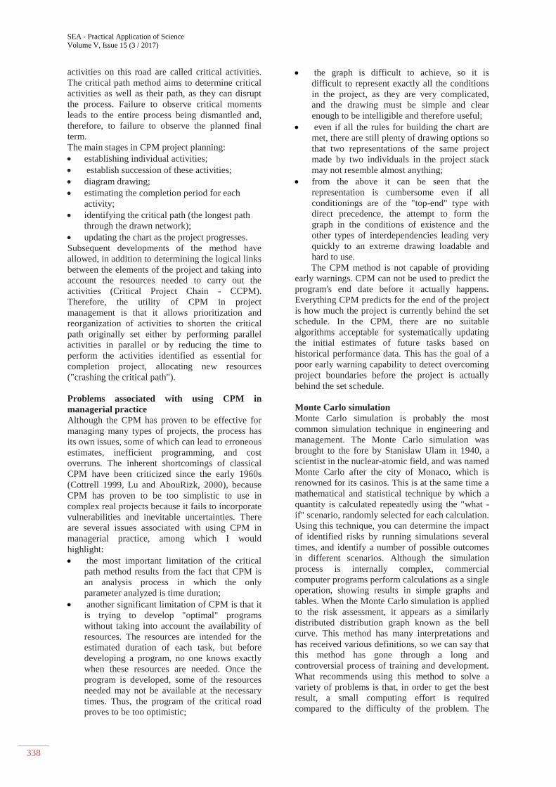
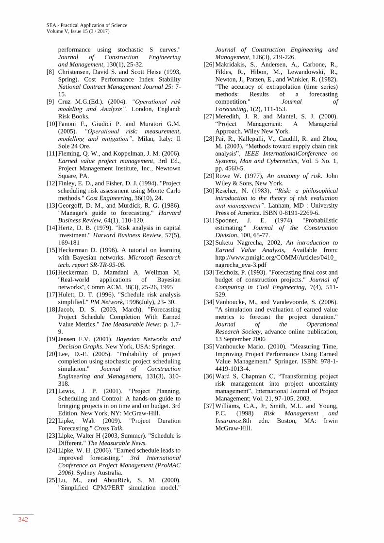
adjacent arcs. By means of such graphs, it is possible to model
operational or decisional managerial processes,
such as transport networks. The structure of such a
process can be represented by a graph as in the
Figure 3. Every graph has a start and end time between
which there are many roads and the one with the
longest length is called a critical road. By the way
is meant a sequence of arcs, ie activities so that the
termination of one coincides with the beginning of
another. A road is considered complete when it
leaves the initial node and reaches the final node.
The length of a road is the sum of the activities that
make up that road. The critical road is the full
length path or the succession of activities that gives
the minimum total duration of the process. The
X = x1,x2,x3,x4
Г(x1) = x2, x4
Г(x2) = x1,x3,x4
Г(x3) = x1
Г(x4) = x2
SEA - Practical Application of Science
Volume V, Issue 15 (3 / 2017)
338
activities on this road are called critical activities.
The critical path method aims to determine critical
activities as well as their path, as they can disrupt
the process. Failure to observe critical moments
leads to the entire process being dismantled and,
therefore, to failure to observe the planned final
term.
The main stages in CPM project planning:
• establishing individual activities;
• establish succession of these activities;
• diagram drawing;
• estimating the completion period for each
activity;
• identifying the critical path (the longest path
through the drawn network);
• updating the chart as the project progresses.
Subsequent developments of the method have
allowed, in addition to determining the logical links
between the elements of the project and taking into
account the resources needed to carry out the
activities (Critical Project Chain - CCPM).
Therefore, the utility of CPM in project
management is that it allows prioritization and
reorganization of activities to shorten the critical
path originally set either by performing parallel
activities in parallel or by reducing the time to
perform the activities identified as essential for
completion project, allocating new resources
("crashing the critical path").
Problems associated with using CPM in
managerial practice Although the CPM has proven to be effective for
managing many types of projects, the process has
its own issues, some of which can lead to erroneous
estimates, inefficient programming, and cost
overruns. The inherent shortcomings of classical
CPM have been criticized since the early 1960s
(Cottrell 1999, Lu and AbouRizk, 2000), because
CPM has proven to be too simplistic to use in
complex real projects because it fails to incorporate
vulnerabilities and inevitable uncertainties. There
are several issues associated with using CPM in
managerial practice, among which I would
highlight:
• the most important limitation of the critical
path method results from the fact that CPM is
an analysis process in which the only
parameter analyzed is time duration;
• another significant limitation of CPM is that it
is trying to develop "optimal" programs
without taking into account the availability of
resources. The resources are intended for the
estimated duration of each task, but before
developing a program, no one knows exactly
when these resources are needed. Once the
program is developed, some of the resources
needed may not be available at the necessary
times. Thus, the program of the critical road
proves to be too optimistic;
• the graph is difficult to achieve, so it is
difficult to represent exactly all the conditions
in the project, as they are very complicated,
and the drawing must be simple and clear
enough to be intelligible and therefore useful;
• even if all the rules for building the chart are
met, there are still plenty of drawing options so
that two representations of the same project
made by two individuals in the project stack
may not resemble almost anything;
• from the above it can be seen that the
representation is cumbersome even if all
conditionings are of the "top-end" type with
direct precedence, the attempt to form the
graph in the conditions of existence and the
other types of interdependencies leading very
quickly to an extreme drawing loadable and
hard to use.
The CPM method is not capable of providing
early warnings. CPM can not be used to predict the
program's end date before it actually happens.
Everything CPM predicts for the end of the project
is how much the project is currently behind the set
schedule. In the CPM, there are no suitable
algorithms acceptable for systematically updating
the initial estimates of future tasks based on
historical performance data. This has the goal of a
poor early warning capability to detect overcoming
project boundaries before the project is actually
behind the set schedule.
Monte Carlo simulation
Monte Carlo simulation is probably the most
common simulation technique in engineering and
management. The Monte Carlo simulation was
brought to the fore by Stanislaw Ulam in 1940, a
scientist in the nuclear-atomic field, and was named
Monte Carlo after the city of Monaco, which is
renowned for its casinos. This is at the same time a
mathematical and statistical technique by which a
quantity is calculated repeatedly using the "what -
if" scenario, randomly selected for each calculation.
Using this technique, you can determine the impact
of identified risks by running simulations several
times, and identify a number of possible outcomes
in different scenarios. Although the simulation
process is internally complex, commercial
computer programs perform calculations as a single
operation, showing results in simple graphs and
tables. When the Monte Carlo simulation is applied
to the risk assessment, it appears as a similarly
distributed distribution graph known as the bell
curve. This method has many interpretations and
has received various definitions, so we can say that
this method has gone through a long and
controversial process of training and development.
What recommends using this method to solve a
variety of problems is that, in order to get the best
result, a small computing effort is required
compared to the difficulty of the problem. The
SEA - Practical Application of Science
Volume V, Issue 15 (3 / 2017)
339
simulation of economic decisions can be applied to
all classes of issues that include operating rules,
policies and procedures such as those on adapting
and controlling decisions. Solving problems with
simulation techniques involves the use of iterative
algorithms and the existence of well-defined steps
to achieve the supposed objective. Input data are
usually random variables obtained by generating
them by a random number generator. Monte Carlo
method is based on the use of such random
variables, because for models involving a large
number of decision variables, the method
necessarily uses computing techniques, and the
algorithm of the method is presented in the
sequence of its interactive steps.
In approaching large-scale industrial projects as
complex nonlinear systems, Monte Carlo method
studies the uncertainties associated with some
variables in the random number system of the
probability distributions estimated for these
variables. Monte Carlo simulation begins with
sketching a set of random numbers for the variables
considered, then a deterministic analysis is
performed to obtain a result based on the set of
random variable values. Monte Carlo simulation
repeats these two steps until significant statistical
results can be obtained.
The main steps of Monte Carlo method are as
follows:
• Identify the most significant variables or
components of the model;
• Determine a measure of the efficacy of the
variables of the studied model;
• Shows the cumulative probability distributions
of the model;
• Set random number rows that are in direct
correspondence with the cumulative
probability distributions of each variable;
• Set random number rows that are in direct
correspondence with the cumulative
probability distributions of each variable;
• Based on the examination of the obtained
results the possible solutions of the problem
are determined;
• A set of random numbers is generated using
random number tables;
• Using each random number and probability
distribution, the values of each variable are
determined;
• Calculate the variable functional value of the
performance;
• Repeat the tests in steps 6 and 8 for each
possible solution;
• Based on the results obtained, a decision on the
optimal solution is made.
Limitations of the Monte Carlo simulation
Because of the complexity of calculating the total
duration of a project resulting from probabilistic
estimates of the component work packages, the
Monte Carlo simulation has been extensively
investigated by several researchers (Finley and
Fisher 1994; Hulett 1996, Lee 2005, Lu and
AbouRizk 2000). For example, Barraza et al.
(2004) conducted a probability forecasting of
project duration and cost using Monte Carlo
simulation. In the study, the correlation between
the past and the future of performance is simplified
by adjusting the probability distribution parameters
of future activities with performance indices (eg
CPI as defined in the earned value method) of the
completed work, resulting in a series of limitations
as follows:
• In order to run the Monte Carlo simulation, it
is necessary to enter three estimates for an
activity, so the results depend on the quality of
the introduced estimates;
• Monte Carlo simulation shows the likelihood
of completing the tasks, it is not the time
actually considered to complete the task;
• Monte Carlo simulation technique can not be
applied to a single task or activity. Project
management requires all activities, as well as
the risk assessment completed for each
activity;
• Running Monte Carlo simulation requires the
purchase of a software program.
Although Monte Carlo Simulation presents a
number of limitations, it remains, however, an
instrument and at the same time a technique used in
the process of quantitative analysis of internal risks
arising in the implementation of projects and which
can provide their managers with a starting point in
the process project planning and execution, but it
should be noted that this technique does not
provide any warning signals to managers about
uncertainties, risks and changes in the external
environment.
USING COMPLEMENTARY TECHNIQUES
TO GENERATE WARNING SIGNALS
ABOUT THE CAUSAL RELATIONSHIP
BETWEEN SOURCES OF UNCERTAINTIES,
RISKS AND PROJECT PARAMETERS -
BAYESIAN NETWORKS.
Bayesian Networks (BN) are recognized as a
mature formalism for managing causality and
uncertainty (Heckerman et al, 1995). Known as
belief networks, causal probabilistic networks,
probability charts, probability-cause models...,
Bayesian Networks provide decision support in
project management for a wide range of issues
involving uncertainty and probabilistic reasoning,
being often used to analyze causal relationships
between different entities. In the field of project
management, Bayesian Networks are a useful tool
for multivariate and integrated risk analysis, for
monitoring and evaluating intervention strategies
SEA - Practical Application of Science
Volume V, Issue 15 (3 / 2017)
340
(through a graphical decision) as well as for their
mitigation (Jensen, 2001, Alexander, 2003).
According to Bayesian approach, project risk can
be defined as the possibility that something is
happening with an impact on objectives and is
measured in terms of probability combinations of
an event (frequency) and its consequences
(impact). To estimate the frequency and impact
distributions, both, historical data and expertise are
used (Cruz, 2004). In this context, Bayesian
networks can be a useful tool to integrate historical
data with those from experts, which can be
qualitative or quantitative (Fanoni, Giudici, and
Muratori, 2005).
The main advantages of Bayesian networks that
can make them suitable for project planning and
execution are:
• the explicit quantification of uncertainties and
the modeling of the causal relationship between
variables;
• Provides reason-to-cause and cause-to-effect
reasoning (propagation is both "forward" and
"backward")
• Ensures the possibility of overturning previous
beliefs in the light of new data;
• Can make predictions with incomplete data;
• Combines subjective and objective data;
• Allows users to make judgments based on
reasoned audits.
Bayesian networks are defined as a graph pattern
that effectively encodes the common probability
distribution for a large set of variables. (Pai et al.,
2003). In a Bayesian network, nodes represent
random variables, and edges represent conditional
dependencies. Nodes that are not connected
represent variables that are conditionally
independent of each other (Heckerman, 1996).
Each node is associated with a probability function
that has as input a set of values for the parent node
variables and gives the probability of the variable
represented by the node (Jensen, 2001; Heckerman,
1996).
The Bayesian Networks are a graphical method of
knowledge representation that uses mathematical
probability theory to model uncertainty over
information and various aspects of interest.
Bayesian networks are defined by graphs, which
have associated probability tables and which are
used to model and reason with uncertainties. The
main purpose of the Bayesian reasoning is to
recalculate the probabilities associated with the
variables taking into account the new observed
events and to exploit the assumptions of
interdependence between the variables to make the
calculations more efficient. Causal or inferential
networks are used in a number of domains to
represent patterns of influence between variables.
In general, causality can be regarded as any
relationship of natural order in which the
knowledge of an event influences the opinion on
another event. This influence can be logical,
physical, in time, or simply conceptual.
A Bayesian network is a network of nodes
connected by links oriented to a probability
function attached to each node. The network (or
graph) of a BN is a directed aciclic graph (DAG),
where there is no targeted start-up path ending in
the same node. If a node has no parent (for
example, there is no link to it), the node will
contain a marginal probability table. If a node has
parents (for example, one or more links to it), the
node contains a conditional probability table
(CPT). Formally, a Bayesian network can be
defined as follows: Bayesian network is a pair (G,
P) where G = (V, E) is an acyclic oriented graph
(DAG) over a finite set of nodes vertices, V,
interconnected by directed links (or margins), E, P
and is a set of probability distributions
(conditional). Each node represents a variable A
with a parent nodes representing variables B1, B2,
..., Bn is assigned a conditional probability table
(CPT) representing P (A | B1, B2, ..., Bn). Nodes
are random variables and links are probabilistic
dependencies between variables. These
dependencies are quantified by a set of conditional
probability tables (CPTs); each variable is assigned
a CPT. For parentless variables, this is an
unconditional distribution (also called marginal). In
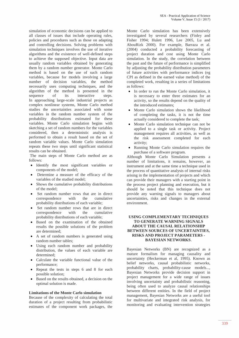
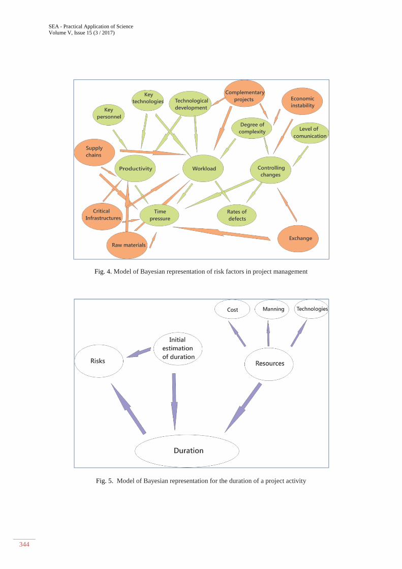
line with the definitions and data above definition,
the network of external and internal risk factors is
presented in the Figure nr. 4. Once we have built
the BN analysis model, we can predict the
probability of risk, which can help us to take
precautionary measures to reduce the risks in large-
scale industrial projects. The most popular software
used to perform the above-mentioned process in
building BN is Hugin Expert. While running
projects, we usually encounter all sorts of issues,
such as finding the origin of the problem. Because
BN can calculate posterior probability, BN can help
find the root of the problem. As an effective
mathematical model of probability deduction,
Bayesian networks have many advantages in risk
control in projects. In project implementation
process, real-time risk analysis is essential to
estimate the impact on project deadlines and
quality. At the same time, we can assess the effect
of optional measures to determine the best
decision-making strategy. Using the advantages of
the Bayesian backsight capability, combined with
implementation situations, we can quickly identify
and analyze the risk factors that lead to project
delay, downsizing or cost overruns, so action can
be taken quickly. In addition, Bayesian network
structures are suited to the changing features of risk
factors in projects due to their light expansiveness
and strong self-learning ability. So, applying
Bayesian networks for risk factor analysis in
projects is more appropriate and more viable than
other methods, as the results from this method are
SEA - Practical Application of Science
Volume V, Issue 15 (3 / 2017)
341
appropriate for real situations. Figure 5 shows a
Bayesian network model built to model sources of
uncertainty as well as how they affect the duration
of a particular activity in a large-scale complex
industrial project. The model contains variables
that capture the uncertain nature of the duration of
an activity or activity. The "Early Estimation of
Duration" of an activity is based on historical data,
past experiences, or expert judgment. "Resources"
include any factor that may increase or decrease the
duration of the activity. Each node is ranked, which
for simplicity is limited to three levels: low,
medium and high. The resource level can be
deduced from the so-called "indicator" nodes.
Therefore, the causal link is from "resources" to the
values of the indicators, such as the "cost", the
available "people" experience and the level of
"technology" available. An important and new
aspect of this approach is to allow the model to be
adapted to use any indicators that are available.
The advantage of this model (BN) is a better
understanding by presenting the results in different
scenarios. It is possible to introduce observations
anywhere in the model to perform not just
predictions, but also several types of compromise
and explanatory analysis. So, for example, we can
introduce observations for the 'Early Estimate of
Duration' and 'Resources' and let the model show
the 'duration' distributions.
CONCLUSIONS
Bayesian networks can be used to predict internal
progress correlated with external volatile factors to
obtain early confidence testimonies. There are at
least three reasons why Bayesian Networks are to
be applied in large complex industrial projects.
First, Bayesian Networks provide useful
predictions, while CPM and EVM can not do so.
Predictive limits indicate the range of possible
results at a given confidence level. Secondly,
Bayesian Networks not only share EVM merits, but
they can provide stable forecasts from the outset of
the project and do not require a stabilization period.
This feature can be attributed to the adaptive nature
of Bayesian networks. EVM forecasts show
significant variability in a project, as predictions
are made only on the basis of small real data
samples. On the contrary, the Bayesian Networks
predict both real data and performance information
in project plans, historical data, and subjective
judgments. The more the project progresses, the
influence of the prior information decreases and the
forecasts become more influenced by the actual
performance data. Like EVM, Bayesian Networks
are universally applicable to a wide range of
projects Thirdly, Bayesian Networks allow users to
adjust the sensitivity of forecasts to actual
performance data based on their confidence in the
accuracy of performance metrics. Measurement
errors are almost inherent in project management
due to human errors, insufficient norms for
determining the value gained, and variations in
reporting ranges. As a result, the level of accuracy
of actual performance data may vary from project
to project. Therefore, Bayesian network flexibility
in relation to measurement errors will be useful in
real projects under various circumstances.
Summary conclusions:
Although the analysis of each forecasting method
has been finalized with its findings from early
warning point of view, the major findings of this
study are:
• EVM predictions can be used to obtain
reliable warnings after project performance is
stabilized;
• The CPM is not capable of providing early
warnings due to its retrospective nature;
• Bayesian networks can be used to forecast
progress and obtain early confidence
testimonies for all types of projects, regardless
of size and complexity;
• Early warning capability of predictive
methods should be evaluated and compared to
the timeliness and reliability of the warning in
the context of early warning systems.
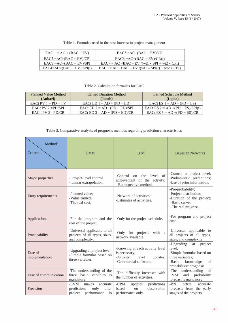
• A full comparative analysis of prognosis
methods regarding prediction characteristics is
done within Table 3.
REFERENCES
[1] Al-Tabtabai, H., and Diekmann, J. E. (1992).
"Judgemental forecasting in construction
projects." Construction Management &
Economics, 10(1), 19.
[2] Anbari, Frank T. (2003, December). “Earned
Value Project Management Method and
Extensions. ”Project Management Journal
34.4: 12-23.
[3] Anbari, Frank T. (2001). “Applications and
Extensions to the Earned Value Analysis
Method.”Proceedings of the Project
Management Institute 2001 Seminars &
Symposium.
[4] Ang, A. H., and Tang, W. H. (1975).
Probability concepts in engineering and
design, John Wiley & Sons, New York, NY
[5] Ayyub, B.M., (2003), “Risk analysis in
engineering and economics”. Boca Raton, FL:
Chapman & Hall/CRC Press, ISBN 1 - 58488-
395-2.
[6] Barr, Zeev (1996, December). "Earned Value
Analysis: A Cast Study." PM Network, pp. 31-
37.
[7] Barraza, G. A., Back, W. E., and Mata, F.
(2004). "Probabilistic forecasting of project
SEA - Practical Application of Science
Volume V, Issue 15 (3 / 2017)
342
performance using stochastic S curves."
Journal of Construction Engineering
and Management, 130(1), 25-32.
[8] Christensen, David S. and Scott Heise (1993,
Spring). Cost Performance Index Stability
National Contract Management Journal 25: 7-
15.
[9] Cruz M.G.(Ed.). (2004). “Operational risk
modeling and Analysis”. London, England:
Risk Books.
[10] Fanoni F., Giudici P. and Muratori G.M.
(2005). “Operational risk: measurement,
modelling and mitigation”. Milan, Italy: Il
Sole 24 Ore.
[11] Fleming, Q. W., and Koppelman, J. M. (2006).
Earned value project management, 3rd Ed.,
Project Management Institute, Inc., Newtown
Square, PA.
[12] Finley, E. D., and Fisher, D. J. (1994). "Project
scheduling risk assessment using Monte Carlo
methods." Cost Engineering, 36(10), 24.
[13] Georgoff, D. M., and Murdick, R. G. (1986).
"Manager's guide to forecasting." Harvard
Business Review, 64(1), 110-120.
[14] Hertz, D. B. (1979). "Risk analysis in capital
investment." Harvard Business Review, 57(5),
169-181
[15] Heckerman D. (1996). A tutorial on learning
with Bayesian networks. Microsoft Research
tech. report SR-TR-95-06.
[16] Heckerman D, Mamdani A, Wellman M,
''Real-world applications of Bayesian
networks'', Comm ACM, 38(3), 25-26, 1995
[17] Hulett, D. T. (1996). "Schedule risk analysis
simplified." PM Network, 1996(July), 23- 30.
[18] Jacob, D. S. (2003, March). "Forecasting
Project Schedule Completion With Earned
Value Metrics." The Measurable News: p. 1,7-
9.
[19] Jensen F.V. (2001). Bayesian Networks and
Decision Graphs. New York, USA: Springer.
[20] Lee, D.-E. (2005). "Probability of project
completion using stochastic project scheduling
simulation." Journal of Construction
Engineering and Management, 131(3), 310-
318.
[21] Lewis, J. P. (2001). “Project Planning,
Scheduling and Control: A hands-on guide to
bringing projects in on time and on budget. 3rd
Edition. New York, NY: McGraw-Hill.
[22] Lipke, Walt (2009). "Project Duration
Forecasting." Cross Talk.
[23] Lipke, Walter H (2003, Summer). "Schedule is
Different." The Measurable News.
[24] Lipke, W. H. (2006). "Earned schedule leads to
improved forecasting." 3rd International
Conference on Project Management (ProMAC
2006). Sydney Australia.
[25] Lu, M., and AbouRizk, S. M. (2000).
"Simplified CPM/PERT simulation model."
Journal of Construction Engineering and
Management, 126(3), 219-226.
[26] Makridakis, S., Andersen, A., Carbone, R.,
Fildes, R., Hibon, M., Lewandowski, R.,
Newton, J., Parzen, E., and Winkler, R. (1982).
"The accuracy of extrapolation (time series)
methods: Results of a forecasting
competition." Journal of
Forecasting, 1(2), 111-153.
[27] Meredith, J. R. and Mantel, S. J. (2000).
“Project Management: A Managerial
Approach. Wiley New York.
[28] Pai, R., Kallepalli, V., Caudill, R. and Zhou,
M. (2003), “Methods toward supply chain risk
analysis”, IEEE InternationalConference on
Systems, Man and Cybernetics, Vol. 5 No. 1,
pp. 4560-5.
[29] Rowe W. (1977), An anatomy of risk. John
Wiley & Sons, New York.
[30] Rescher, N. (1983), “Risk: a philosophical
introduction to the theory of risk evaluation
and management”. Lanham, MD : University
Press of America. ISBN 0-8191-2269-6.
[31] Spooner, J. E. (1974). "Probabilistic
estimating." Journal of the Construction
Division, 100, 65-77.
[32] Suketu Nagrecha, 2002, An introduction to
Earned Value Analysis, Available from:
http://www.pmiglc.org/COMM/Articles/0410_
nagrecha_eva-3.pdf
[33] Teicholz, P. (1993). "Forecasting final cost and
budget of construction projects." Journal of
Computing in Civil Engineering, 7(4), 511-
529.
[34] Vanhoucke, M., and Vandevoorde, S. (2006).
"A simulation and evaluation of earned value
metrics to forecast the project duration."
Journal of the Operational
Research Society, advance online publication,
13 September 2006
[35] Vanhoucke Mario. (2010). "Measuring Time,
Improving Project Performance Using Earned
Value Management." Springer. ISBN: 978-1-
4419-1013-4.
[36] Ward S, Chapman C, “Transforming project
risk management into project uncertainty
management”, International Journal of Project
Management; Vol. 21, 97-105, 2003.
[37] Williams, C.A., Jr, Smith, M.L. and Young,
P.C. (1998) Risk Management and
Insurance.8th edn. Boston, MA: Irwin
McGraw-Hill.
SEA - Practical Application of Science
Volume V, Issue 15 (3 / 2017)
343
ANNEXES
Fig. 1. EVM elements, adapted from Lipke W., 2003, page 2.
Fig. 2. Math graph representation model for CPM
Fig. 3. Graph model for managerial processes.
SEA - Practical Application of Science
Volume V, Issue 15 (3 / 2017)
344
Fig. 4. Model of Bayesian representation of risk factors in project management
Fig. 5. Model of Bayesian representation for the duration of a project activity
SEA - Practical Application of Science
Volume V, Issue 15 (3 / 2017)
345
Table 1. Formulas used in the cost forecast in project management
EAC 1 = AC + (BAC − EV) EAC5 =AC+(BAC − EV)/CR
EAC2 =AC+(BAC − EV)/CPI EAC6 =AC+(BAC − EV)/CR(t)
EAC3 =AC+(BAC − EV)/SPI EAC7 = AC +BAC – EV /(wt1 ∗ SPI + wt2 ∗ CPI)
EAC4=AC+(BAC − EV)/SPI(t) EAC8 = AC +BAC – EV /(wt1 ∗ SPI(t) + wt2 ∗ CPI)
Table 2. Calculation formulas for EAC
Table 3. Comparative analysis of prognosis methods regarding prediction characteristics
Methods
Criteria EVM CPM Bayesian Networks
Major properties
- Project-level control.
- Linear extrapolation.
-Control on the level of
achievement of the activity;
- Retrospective method.
-Control at project level;
-Probabilistic predictions;
-Use of prior information.
Entry requirements
-Planned value;
-Value earned;
-The real cost.
-Network of activities;
-Estimates of activities.
-Pre-probability;
-Project distribution;
-Duration of the project;
-Basic curve;
-The real progress.
Applications
-For the program and the
cost of the project.
-Only for the project schedule.
-For program and project
cost.
Practicability
-Universal applicable to all
projects of all types, sizes,
and complexity.
-Only for projects with a
network available.
-Universal applicable to
all projects of all types,
sizes, and complexity.
Ease of
implementation
-Upgrading at project level;
-Simple formulas based on
three variables.
-Knowing at each activity level
is necessary;
-Activity level updates.
-Commercial software.
-Upgrading at project
level;
-Simple formulas based on
three variables;
-Basic knowledge of
probabilistic prognosis.
Ease of communication
-The understanding of the
three basic variables is
mandatory.
-The difficulty increases with
the number of activities.
-The understanding of
EVM and probability
forecast is mandatory.
Precision
-EVM makes accurate
predictions only after
project performance is
-CPM updates predictions
based on observation
performance only.
-BN offers accurate
forecasts from the early
stages of the projects.
Planned Value Method
(Anbari)
Earned Duration Method
(Jacob)
Earned Schedule Method
(Lipke)
EACt PV 1 = PD − TV EACt ED 1 = AD + (PD − ED) EACt ES 1 = AD + (PD − ES)
EACt PV 2 =PD/SPI EACt ED 2 = AD +(PD − ED)/SPI EACt ES 2 = AD +(PD − ES)/SPI(t)
EAC t PV 3 =PD/CR EACt ED 3 = AD + (PD − ED)/CR EACt ES 3 = AD +(PD − ES)/CR

SEA - Practical Application of Science
Volume V, Issue 15 (3 / 2017)
346
stabilized.
The opportunity to
warning
-EVM offers early
warnings, but EVM can
only be applied after
project performance
stabilizes.
-CPM almost does not offer any
warnings
-BN generates early
warnings from the
planning stage.
Flexibility
-Predictions can be
adjusted with various
performance factors that
can be chosen by the user.
The results are deterministic.
-Sensitivity of real data
predictions can be
modified by the likelihood
of variation of terms.
Recommended